Hierarchical Testing in the High-Dimensional Setting with Correlated Variables

Abstract

We propose a method for testing whether hierarchically ordered groups of potentially correlated variables are significant for explaining a response in a high-dimensional linear model. In presence of highly correlated variables, as is very common in high-dimensional data, it seems indispensable to go beyond an approach of inferring individual regression coefficients, and we show that detecting smallest groups of variables (MTDs: minimal true detections) is realistic. Thanks to the hierarchy among the groups of variables, powerful multiple testing adjustment is possible which leads to a data-driven choice of the resolution level for the groups. Our procedure, based on repeated sample splitting, is shown to asymptotically control the familywise error rate and we provide empirical results for simulated and real data which complement the theoretical analysis. Supplementary materials for this article are available after the References.

Keywords and phrases: Familywise error rate; Hierarchical clustering; High-dimensional variable selection; Lasso; Linear model; Minimal true detection; Multiple testing; Sample splitting.

1 Introduction

High-dimensional statistical inference where the number $p$ of (co-)variables might be much larger than the sample size $n$ has become a key issue in many areas of applications. We focus here on the linear model

$$\mathbf{Y}=\mathbf{X}\beta^{0}+\varepsilon,\ \varepsilon\sim{\cal N}_{n}(0,\sigma^{2}I)$$ (1)

with $n\times p$ design matrix $\mathbf{X}$, $p\times 1$ regression vector $\beta^{0}$ and $n\times 1$ response $\mathbf{Y}$, allowing for high-dimensionality with $p\gg n$. Often, the active set of variables carrying the relevant information

$$S_{0}=\{j;\beta^{0}_{j}\neq 0\}$$

is assumed to be a small subset of all variables, i.e., the model is sparse with many $\beta^{0}_{j}$ being equal to zero. Our main goal is testing of significance of groups of parameters: for a group or cluster $C\subseteq\{1,\ldots,p\}$,

$$H_{0,C}:\ \beta^{0}_{j}=0\ \mbox{for all}\ j\in C,\ \ \ H_{A,C}:\ \beta^{0}_{j}\neq 0\ \mbox{for at least one}\ j\in C.$$

Significance testing in the high-dimensional framework is essential when looking beyond point estimation. Wasserman and Roeder, (2009) propose an approach based on single sample splitting, and Meinshausen et al., (2009) improve the reliability and power of the method based on multiple sample splitting. Minnier et al., (2011) consider a perturbation technique, and (modified) bootstrap-type schemes are analyzed by Chatterjee and Lahiri, (2013) and Liu and Yu, (2013). Another line of methods have been proposed using low-dimensional regularized projections (e.g. on single variables for individual hypotheses $H_{0,j}$) which have some optimality properties (Zhang and Zhang,, 2014; Bühlmann,, 2013; Javanmard and Montanari, 2014b, ; van de Geer et al.,, 2014; Javanmard and Montanari, 2014a, ). However, in presence of highly correlated variables, all these methods are likely to fail for testing individual hypotheses $H_{0,j}$.

An interesting way to address the fundamental limitation of identifiability in presence of high correlation or near linear dependence is given by a hierarchical testing scheme proposed by Meinshausen, (2008). First, the variables are grouped in a hierarchical way, for example by hierarchical clustering. At the top of the hierarchy, the global hypothesis $H_{0,\{1,\ldots,p\}}$ is tested. If it can be rejected, a finer partition with clusters $\{C_{k}\}_{k}$ is considered, and for the ones where $H_{0,C_{k}}$ can be rejected, one proceeds down the hierarchy to finer partitions. The method has the powerful advantage that it automatically goes (from top to bottom in the hierarchy) to finer resolution with smaller clusters, depending on signal-strength and the correlation structure among the variables. At the end, significant clusters can be typically found, and if the signal for an individual variable is sufficiently strong, even significance of a single variable can be detected. Meinshausen, (2008) has worked out a simple yet powerful way for controlling the familywise error rate when performing multiple tests in the hierarchy, assuming that there is a method which leads to valid p-values for the various hypotheses tests; for example, when $p<n$ and with Gaussian errors, one can use partial F-tests.

1.1 Our contribution

As one of our main contributions, we deal here with the problem to obtain valid p-values for hypotheses $H_{0,C}$ where $C$ is an arbitrary group of (typically highly correlated) variables, for the high-dimensional scenario where $p\gg n$. We address this important and open issue; note that testing the global null-hypothesis $H_{0,\{1,\ldots,p\}}$, in contrast to the “partial” hypothesis $H_{0,C}$ for some $C$ with cardinality $1<|C|<p$, is a rather different issue and has been addressed before (Goeman et al.,, 2006, cf.). Once we have valid p-values for $H_{0,C}$ for a arbitrary groups $C$, we make use of the method from Meinshausen, (2008) leading to non-asymptotic bounds for strong control of the familywise error rate in a hierarchical structure. For construction of the p-values, we rely on multiple sample splitting (Meinshausen et al.,, 2009). While this might be sub-optimal from a theoretical perspective, especially with respect to power, the method seems to perform well in a larger empirical study for individual hypotheses $H_{0,j}\ (j=1,\ldots,p)$ in terms of reliable control of the familywise error rate in multiple testing (Dezeure et al.,, 2014). We also extend the Shaffer improvement in Meinshausen, (2008, Section 3.6) to the high-dimensional scenario, increasing the power of the hierarchical method such that detection of more singletons than with the method from (Meinshausen et al.,, 2009) becomes possible.

Our second main contribution is the development of new methodology and theory for hierarchical inference and testing of hypotheses, using multiple sample splitting techniques (and multiple sample splitting is important for reproducibility (Meinshausen et al.,, 2009)). Regarding methodology, the hierarchical approach allows for a substantially higher number of so-called minimal true detections (MTDs: significant smallest groups of variables) than the single variable analogue and has the remarkable property of adaptively selecting a best resolution level (MTDs with the smallest possible cardinality). We prove strong control of the familywise error rate of the hierarchical method under a “zonal assumption” which is weaker than the standard $\beta$-min condition (used in Meinshausen et al., (2009)), that is, we do not require that all non-zero coefficients in the parameter-vector $\beta^{0}_{j}$ are sufficiently large. We demonstrate the finite sample behavior of the method with various empirical results.

We note that recently, Meinshausen, (2013) describes another procedure for dealing with highly correlated variables and hierarchical testing of groups or clusters of variables. His method is an interesting alternative with the remarkable property that it does not require (major) regularity assumptions on the design matrix. The procedure is taking advantage of the special structure of a linear model while our approach is: (i) more generic and conceptually applicable to other (e.g. generalized linear) models, and (ii) computationally much more efficient due to variable screening in a first stage.

1.2 Outline of the paper

In Section 2 we describe our method for obtaining p-values for groups of variables and its use for hierarchical testing in high-dimensional settings. We show in Section 3 that the familywise error rate (FWER) is strongly controlled, and we describe a Shaffer improvement to increase the method’s power while keeping control over the FWER. Section 4 is devoted to empirical results: we show that our procedure improves the single variable testing method of Meinshausen et al., (2009) in settings with strong correlation among certain variables, particularly with respect to minimal true detections (MTDs). In Section 5 we provide theoretical evidence that the FWER is controlled even if a “screening assumption” required in Section 3 is not satisfied.

2 Description of method

Our method is based on four main steps: (i) hierarchical clustering of the variables, (ii) variable screening in a linear model, (iii) significance testing (with multiplicity adjustment) based on sample splitting, and (iv) aggregation over multiple sample splits and hierarchical multiplicity adjustment. See also Section 2.5 for a schematic summary.

2.1 Clustering

In a first step, we construct a hierarchy of clusters. A hierarchy, which can be represented as a tree-graph, $\mathcal{T}$ is a set of clusters $\{C_{k}\}_{k}$ with $C_{k}\subseteq\{1,\dots,p\}$: the root node of the tree $\{1,\dots,p\}$ contains all variables and for any two clusters $C_{k},C_{k^{\prime}}\in\mathcal{T}$, either one cluster is a subset of the other, or they have an empty intersection. We use the notation $\mbox{pa}(C)$ for the parent of a cluster $C$, (the smallest superset of $C$), $\mbox{ch}(C)$ for the children of a cluster $C$ (all clusters that have $C$ as parent). Cluster $C$ is called an ancestor of cluster $D$ if $D\subset C$.

As noted in Meinshausen, (2008), the hierarchy can be derived from specific domain knowledge or in some other natural way. The philosophy of the method is that highly correlated variables (or variables which are nearly linearly dependent) should end up in a single small cluster: it will then be relatively easy to identify the cluster as relevant, if it contains at least some variables from the active set $S_{0}$. For our empirical results, we consider standard hierarchical clustering based on correlation between variables, or a novel hierarchical scheme using canonical correlations between clusters (Bühlmann et al.,, 2013).

Once the hierarchical structure is given, the method goes on with a hierarchical version of the multi sample-splitting procedure from Meinshausen et al., (2009). The following two steps, described in Sections 2.2 and 2.3 have to be repeated for each sample split, indexed by $b=1,\ldots,B$ where $B$ is the number of sample splits (since $B>1$, we use the terminology multi sample-splitting).

2.2 Screening

The original data of sample size $n$ is split into two disjoint groups, $N_{in}^{(b)}$ and $N_{out}^{(b)}$, i.e. a split $\{1,\dots,n\}=N_{in}^{(b)}\cup N_{out}^{(b)}$ is chosen. The groups are chosen of equal size if $n$ is even or satisfy $|N_{out}^{(b)}|=|N_{in}^{(b)}|+1$ if $n$ is odd.

Then, using only $N_{in}^{(b)}$, estimate with a screening procedure the set of active predictors $\hat{S}^{(b)}$. A prime example is the Lasso (Tibshirani,, 1996).

2.3 Testing and multiplicity adjustment

By considering for each cluster $C$ in the hierarchy $\mathcal{T}$ its intersection with $\hat{S}^{(b)}$, an induced hierarchy with root $\hat{S}^{(b)}$ is given. Due to this construction, assuming that the cardinality $|\hat{S}^{(b)}|<n/2$, the situation is not high-dimensional anymore. Therefore, on this induced hierarchy, we can apply testing procedure similar as in Meinshausen, (2008), the difference being that the hierarchical adjustment is not performed at this stage but in Section 2.4 after the aggregation over many sample splits.

Based on the other half of the sample $N_{out}^{(b)}$, we use the classical partial F-test with the full model $\hat{S}^{(b)}$ and submodel $C\cap\hat{S}^{(b)}$ for the null hypothesis $H_{0,C\cap\hat{S}^{(b)}}$, where $C\in{\cal T}$ is a given cluster. Thereby, we implicitly assume that the submatrix $\mathbf{X}_{\hat{S}^{(b)}}$ with columns corresponding to $\hat{S}^{(b)}$ is of full rank (since $|\hat{S}^{(b)}|<n/2$). We then assign the p-value from the partial F-test to the entire cluster $C$, although we have only used the variables in $C\cap\hat{S}^{(b)}$. If a cluster $C$ does not contain selected variables from $\hat{S}^{(b)}$, we set the p-value to 1. In summary, we define:

$$p^{C,(b)}=\begin{cases}p_{\mathrm{partial\>F-test}}^{C\cap S^{(b)}}\ \mbox{based on}\ \mathbf{Y}_{N_{out}^{(b)}},\mathbf{X}_{N_{out}^{(b)},\hat{S}^{(b)}}&,\text{if $C\cap\hat{S}^{(b)}\neq\emptyset$},\\ 1&,\text{if $C\cap\hat{S}^{(b)}=\emptyset$,}\end{cases}$$ (2)

Then, for $C\in\mathcal{T}$ define the multiplicity adjusted (non-aggregated) p-value as

$$p_{adj}^{C,(b)}=\min\big{(}\,p^{C,(b)}\frac{|\hat{S}^{(b)}|}{|C\cap\hat{S}^{(b)}|}~{},~{}1\big{)}$$ (3)

if $C\cap\hat{S}^{(b)}\neq\emptyset$ and $p_{adj}^{C,(b)}=1$ otherwise.

2.4 Aggregation and hierarchical adjustment

By repeating the steps in Section 2.2 and 2.3 for $b=1,\dots,B$, we obtain for each cluster $C$ of the hierarchy ${\cal T}$ a set of $B$ p-values $p_{adj}^{C,(1)},\ldots,p_{adj}^{C,(B)}$. We aggregate these p-values by considering their empirical quantile.

For $\gamma\in(0,1)$ define the aggregated p-values

$$Q^{C}(\gamma)=\min\big{\{}\,1~{},~{}q_{\gamma}\big{(}\big{\{}p_{adj}^{C,(b)}/\gamma;\,b=1,\dots,B\big{\}}\big{)}\big{\}},$$

where $q_{\gamma}(\cdot)$ is the (empirical) $\gamma$–quantile function. Finally, define the hierarchically adjusted (aggregated) p-values as

$$Q_{h}^{C}(\gamma)=\max_{D\in\mathcal{T}:C\subseteq D}Q^{D}(\gamma)$$

such that the hierarchically adjusted (aggregated) p-value of a cluster $C$ is always bigger than the hierarchically adjusted (aggregated) p-value of an ancestor cluster. In Section 3 we show that for any fixed $\gamma\in(0,1)$ the $Q_{h}^{C}(\gamma)$ are correct p-values. At this stage, $\gamma$ should be considered as a pre-specified parameter of the method.

Similarly as in Meinshausen et al., (2009), error control is not guaranteed if we optimize over $\gamma$, that is, for each $C$ we would choose the minimal $Q_{h}^{C}(\gamma)$. Nevertheless, it is possible to eliminate parameter $\gamma$ by proceeding as follows. Define

$$P^{C}=\min\big{\{}\,1~{},~{}(1-\log\gamma_{\min})\inf_{\gamma\in(\gamma_{\min},1)}Q^{C}(\gamma)\big{\}},$$ (4)

for a lower bound $\gamma_{\min}\in(0,1)$ for $\gamma$, typically $\gamma_{\min}=0.05$. Then proceed with the hierarchical adjustment of $P^{C}$ by defining

$$P_{h}^{C}=\max_{D\in\mathcal{T}:C\subseteq D}P^{C}.$$

These values $P_{h}^{C}$ are the final output of our method: we will show again in Section 3 that $P_{h}^{C}$ are a valid p-value controlling the familywise error rate when testing over all $C\in\mathcal{T}$.

Our proposed “top-down”: method is schematically summarized in Section 2.5 below. In the Supplemental Material we illustrate a sub-ideal alternative “bottom-up” approach which is empirically found to exhibit substantially less power.

2.5 Schematic summary of the method

We summarize our proposed method with the following schematic description.

Step 1: Clustering

$$\{\mathbf{X}_{1},\dots,\mathbf{X}_{p}\}\hskip 11.38109pt\xrightarrow{\mbox{clustering}}\hskip 11.38109pt\mathcal{T}$$

Repeat for $b=1,\dots,B$:

Step 2: Screening

$$\{1,\dots,n\}=N\hskip 11.38109pt\xrightarrow{\mbox{sample split}}\hskip 11.38109ptN_{in}^{(b)}\cup N_{out}^{(b)}\hskip 11.38109pt\xrightarrow{\mbox{screening}}\hskip 11.38109pt\hat{S}^{(b)}$$

Step 3: Testing and multiplicity adjustment

$$|\hat{S}^{(b)}|<|N_{out}^{(b)}|\hskip 11.38109pt\xrightarrow{\mbox{testing}}\hskip 11.38109ptp^{C,(b)}\hskip 11.38109pt\xrightarrow{\mbox{multiplicity adjustment}}\hskip 11.38109ptp_{adj}^{C,(b)}$$

End of repeating for $b=1,\dots,B$.

Step 4: Aggregation and hierarchical adjustment

$$p_{adj}^{C,(b)}\hskip 11.38109pt\xrightarrow{\mbox{aggregation}}\hskip 11.38109ptQ^{C}(\gamma)\hskip 11.38109pt\xrightarrow{\mbox{hierarchical adjustment}}\hskip 11.38109ptQ^{C}_{h}(\gamma)$$

$$p_{adj}^{C,(b)}\hskip 11.38109pt\xrightarrow{\mbox{aggregation}}\hskip 11.38109ptQ^{C}(\gamma)\hskip 11.38109pt\xrightarrow{\mbox{elimination of }\gamma}\hskip 11.38109ptP^{C}\hskip 11.38109pt\xrightarrow{\mbox{hierarchical adjustment}}\hskip 5.69054ptP^{C}_{h}$$

3 Familywise error rate control

We show in this section, that if the variable selection procedure $\hat{S}$ satisfies two assumptions, then the p-values $Q_{h}^{C}(\gamma)$ and $P_{h}^{C}$ defined in Section 2 control the familywise error rate. The assumptions are:

$$\mbox{(A1) \it{Sparsity property}:}\;|\hat{S}|<n/2.$$

$$\mbox{(A2) \it{$\delta$-Screening property}:}\;\mathbb{P}[\hat{S}\supseteq S_{0}]\geq 1-\delta,\ \mbox{where}\ 0<\delta<1.$$

The sparsity property in (A1) implies that for each sample split $b$ it holds that $|\hat{S}^{(b)}|<|N_{out}^{(b)}|$, a condition which is necessary to apply classical tests. The $\delta$-screening property in (A2) ensures that all the relevant variables are retained with high probability ($\delta$ is typically small). While (A1) is the same condition as in Meinshausen et al., (2009, Section 3.1), we consider with (A2) a slight modification of the assumption in Meinshausen et al., (2009, Section 3.1) in order to obtain non-asymptotic bounds for familywise error rate control. We provide a relaxation of the screening property (A2) in Section 5.

Example. Consider the Lasso as a variable selection method $\hat{S}$. Assumption (A1) holds for any value of the regularization parameter. Assumption (A2) is ensured when requiring the following conditions:

1. The design matrix $\mathbf{X}$ satisfies the compatibility condition with compatibility constant $\phi_{0}^{2}$ (Bühlmann and van de Geer,, 2011, cf. (6.4)). Furthermore, it is normalized such that each column $\mathbf{X}^{(j)}$ satisfies $\|\mathbf{X}^{(j)}\|_{2}^{2}/n=1$ for all $j=1,\ldots,p$.

2. A beta-min condition holds (we use here the notation $s_{0}=|S_{0}|$):

   $$\min_{j\in S_{0}}|\beta^{0}_{j}|>16\sigma\sqrt{\frac{t^{2}+2\log(p)}{n}}s_{0}/\phi_{0}^{2}.$$

Then, the Lasso with regularization parameter $\lambda=4\sigma_{\varepsilon}\sqrt{\frac{t^{2}+2\log(p)}{n}}$ satisfies (A2) with $\delta=2\exp(-t^{2}/2)$ (Bühlmann and van de Geer,, 2011, Lem. 6.2, Thm. 6.1, (2.13)).

Especially when the correlation among the variables is high (violating the compatibility condition in the Example above), one can hardly expect the Lasso or any other variable selection method to satisfy (A2) for very small $\delta$. In Section 4 we present empirical results showing that the hierarchical p-value method still works well even when the screening property is not satisfied for a small value $\delta$, and we provide some supporting theoretical results for this fact in Section 5.

For a given hierarchy $\mathcal{T}$, denote the set of clusters that fulfill the null hypothesis by

$$\mathcal{T}_{0}:=\{C\in\mathcal{T}\,:\,H_{0,C}\mbox{ is fulfilled}\}.$$

Furthermore, for some fixed parameter $\gamma\in(0,1)$ and some fixed significance level $\alpha\in(0,1)$,

$$\mathcal{T}^{\gamma}_{rej}=\{C\in\mathcal{T}\,:\,Q_{h}^{C}(\gamma)\leq\alpha\}$$

is the set of rejected clusters based on the p-values $Q_{h}^{C}(\gamma)$ and analogously,

$$\mathcal{T}_{rej}=\{C\in\mathcal{T}\,:\,P_{h}^{C}\leq\alpha\}$$

is the set of the rejected clusters when considering the p-values $P_{h}^{C}$. The latter does not require to choose or pre-specify a parameter like $\gamma$.

Theorem 1.

Assume that (A1) and (A2) hold. Then for any significance level $\alpha\in(0,1)$ and $B$ denoting the number of sample splits:

1. For any fixed $\gamma\in(0,1)$, the p-values $Q_{h}^{C}(\gamma)$ control the familywise error rate in the sense that:

   $$\mathbb{P}(\mathcal{T}^{\gamma}_{rej}\cap\mathcal{T}_{0}\neq\emptyset)\leq\alpha+1-(1-\delta)^{B}\leq\alpha+B\delta.$$

2. The p-values $P_{h}^{C}$ control the familywise error rate in the sense that:

   $$\mathbb{P}(\mathcal{T}_{rej}\cap\mathcal{T}_{0}\neq\emptyset)\leq\alpha+1-(1-\delta)^{B}\leq\alpha+B\delta.$$

A proof is given in the Supplemental Material. From Theorem 1, providing non-asymptotic bounds for familywise error rate control, one can easily derive asymptotic familywise error control using the assumption

$$\mbox{(A2') \it{Screening property}:}\;\lim_{n\to\infty}\mathbb{P}[\hat{S}\supseteq S_{0}]=1.$$

Example (continued). For the Lasso, under the assumption 1. described in the Example above, and replacing assumption 2. by an asymptotic beta-min condition

$$\min_{j\in S_{0}}|\beta^{0}_{j}|\gg\sqrt{\frac{\log(p)}{n}}s_{0}/\phi_{0}^{2},$$ (5)

we have that (A2’) holds (as $n\to\infty$, $p=p_{n}$ and $s_{0}=s_{0;n}$ and $\phi_{0}^{2}=\phi_{0;n}^{2}$ are allowed to change with $n$).

We then have the following result.

Corollary 1.

Assume that (A1) and (A2’) hold. Then for any fixed $\gamma\in(0,1)$ and significance level $\alpha\in(0,1)$:

$$\limsup_{n\to\infty}\mathbb{P}(\mathcal{T}^{\gamma}_{rej}\cap\mathcal{T}_{0}\neq\emptyset)\leq\alpha$$

$$\limsup_{n\to\infty}\mathbb{P}(\mathcal{T}_{rej}\cap\mathcal{T}_{0}\neq\emptyset)\leq\alpha.$$

3.1 Shaffer improvement in high-dimensional setting

A similar version of the Shaffer improvement as described in Meinshausen, (2008, Section 2.4) can be applied to our method. The main idea, shown by Shaffer, (1986), is that in a hierarchical structure, some combinations of null hypothesis can be excluded a priori, and incorporating constraints on the possible combinations of null hypotheses can increase the power of the method.

Consider a binary hierarchy $\mathcal{T}$ and a screened set $\hat{S}\subset\{1,\dots,p\}$. The siblings of a cluster $C$ are the children of the parent of $C$ which are not identical to $C$, $\mbox{si}(C)=\mbox{ch}(\mbox{pa}(C))\backslash C$. Define the effective cluster size $|C|^{\hat{S}}_{e\!f\!f}$ of the cluster $C\in\mathcal{T}$ restricted to the screened set $\hat{S}$ as

$$|C|^{\hat{S}}_{e\!f\!f}=\left\{\begin{array}[]{ll}|C\cap\hat{S}|,&\mbox{if $\exists\,E\in\mbox{ch}(\mbox{si}(C))$ s.t. $E\cap\hat{S}\neq\emptyset$}\\ |C\cap\hat{S}|+|\mbox{si}(C)\cap\hat{S}|,&\mbox{otherwise.}\end{array}\right.$$

Note that when no screening is performed ($\hat{S}=\{1,\dots,p\}$) this definition coincides with the definition of the effective cluster size in Meinshausen, (2008). Moreover the condition “$\exists\,E\in\mbox{ch}(\mbox{si}(C))$ s.t. $E\cap\hat{S}\neq\emptyset$” is stronger than the condition ”$\mbox{si}(C)$ is not a leaf node“ of Meinshausen, (2008) and hence the improvement given by our definition of restricted cluster size is bigger than the one given by a straightforward adaption of Meinshausen, (2008).

The Shaffer improvement in the high dimensional setting is then given by considering the multiplicity adjustment

$$p_{adj}^{C,(b)}=\min\big{(}\,p^{C,(b)}\frac{|\hat{S}^{(b)}|}{|C|^{\hat{S}^{(b)}}_{e\!f\!f}}~{},~{}1\big{)},$$ (7)

instead of using the multiplicity adjustment in (3).

Obviously, since the effective cluster size is always at least as big as the cluster size, the Shaffer improvement produces smaller p-values and hence increases the power of the method while the familywise error rate control is still guaranteed, as described next.

Theorem 2.

Assume the hierarchy $\mathcal{T}$ is binary. Then, Theorem 1 and Corollary 1 still hold when using the Shaffer improvement (7) as multiplicity adjustment, assuming the conditions of Theorem 1 or Corollary 1, respectively.

A proof is given in the Supplemental Material. We note that an extension of the results in Theorem 1 and 2 to control the false discovery rate (Benjamini and Hochberg,, 1995), instead of the FWER, for hierarchically ordered hypotheses (with corresponding dependent p-values) seems very challenging.

4 Empirical results

In this section we study the performance of our hierarchical method and compare it with the single-variable testing method of Meinshausen et al., (2009). Section 4.3 provides most informative results about our new method, in particular for understanding the differences in comparison to the single-variable approach.

In a simulation study, we consider both synthetic and semi-real data. The former are used to study special designs where we expect one of the two methods to perform clearly better. The semi-real data are used to obtain insights of what happens when the design matrix comes from real high-dimensional datasets. In our simulation study, all the data are generated from a linear model

$$Y=\mathbf{X}\beta^{0}+\varepsilon,$$

where $\mathbf{X}$ is a $n\times p$ matrix from synthetic (designs 1 to 3) or real (designs 4 to 7) data, $\beta^{0}$ is a $p\times 1$ synthetic regression vector and $\varepsilon\sim\mathcal{N}_{n}(0,\sigma^{2}I_{n})$ is a synthetic noise term. The data are always standardized such that $\mathbf{X}$ has columns with empirical mean zero and variance one.

We also apply the two different methods to a real dataset in Section 4.4.

4.1 Implementation of the method

The implementation of our hierarchical method, and also of the single variable procedure from Meinshausen et al., (2009), requires to make some choices. We mostly consider fairly standard and “easy to use” methods; unless there is some deeper methodological difference, as in our choice of additionally considering a less standard clustering procedure.

For clustering we consider the recently proposed canonical correlation clustering of Bühlmann et al., (2013) and the standard hierarchical clustering (using the R-fuction hclust) with distance between two covariables set as 1 less the absolute correlation between the covariables, using complete linkage (other linkages lead to similar results). For variable screening, we use the Lasso (i.e., $\hat{S}$ from the non-zero estimated coefficients from Lasso) with regularization parameter chosen by 10-fold cross-validation.

As in Meinshausen et al., (2009), we choose $B=50$ as the number of sample splits. For aggregation, the p-values $P_{h}^{C}$ in (4) are computed over a grid of $\gamma$-values between $\gamma_{min}=0.05$ and $1$ with grid-steps of size $0.025$. For both hierarchical methods we use the Shaffer improvement described in Section 3.1. As nominal significance level we always consider $\alpha=5\%$.

4.2 Simulation study with synthetic and semi-real data

We consider 42 scenarios based on 7 designs. For each design we consider 6 settings by varying the number of variables $p$ in the model ($p=200$, $p=500$ and $p=1000$) and the signal to noise ratio (SNR, for each design and choice of $p$ we consider a low and a high SNR, namely for $p=200$ we use $\mbox{SNR}=4$ and $\mbox{SNR}=8$, for $p=500$ we use $\mbox{SNR}=8$ and $\mbox{SNR}=16$, for $p=1000$ we use $\mbox{SNR}=16$ and $\mbox{SNR}=32$). The signal to noise ratio is defined by

$$\mbox{SNR}=\sqrt{\frac{(\beta^{0})^{T}\mathbf{X}^{T}\mathbf{X}\beta^{0}}{n\sigma^{2}}}$$

and our choices of signal to noise ratios are avoiding scenarios where the methods have degenerate performance of 0% or 100%, respectively. In designs 1 to 5 the sparsity $s_{0}$ is set to be 10, while in designs 6 and 7 it is set to be 6. The non-zero components of $\beta^{0}$ are randomly set as $\beta_{j}^{0}=1$ or $\beta_{j}^{0}=-1$ for $j\in S_{0}$. The choice of $S_{0}$ is design-specific and hence explained with the descriptions of the designs as follows.

Design 1: equi correlation
We set $n=100$ and generate $\mathbf{X}$ from a centered multivariate normal distribution with equal variances $\rho_{jj}=1$ and covariances equal to $\rho_{jk}=0.3$ between variables $j$ and $k$ for $j\neq k\in\{1,\dots,p\}$. The 10 active variables are chosen randomly among the $p$ covariables.

Design 2: high correlation within small blocks
We set $n=100$ and generate $\mathbf{X}$ from a centered multivariate normal distribution with covariance $\rho_{jk}$ between variables $j$ and $k$ set as $\rho_{jj}=1$ for all $j$, $\rho_{j,j+1}=\rho_{j+1,j}=0.9$ for $j\in\{1,3,5,7,9,11,13,15,17,19\}$ and $\rho_{jk}=0$ otherwise. We choose in each of the 10 two-dimensional blocks with high correlation one active variable, i.e. for $j\in\{1,3,5,7,9,11,13,15,17,19\}$ we choose randomly either $j\in S_{0}$ or $j+1\in S_{0}$.

Design 3: high correlation within large blocks
We set $n=100$ and generate $\mathbf{X}$ from a centered multivariate normal distribution with a block diagonal covariance matrix with 10 $p/10$-dimensional blocks $B_{p/10}(0.9)$ defined by $(B_{p/10}(0.9))_{jj}=1$ and $(B_{p/10}(0.9))_{jk}=0.9$ for $j\neq k$. We randomly choose in each of these p/10-dimensional blocks with high correlation one active variable.

Design 4: Riboflavin dataset with normal correlation
We consider the Riboflavin dataset (Bühlmann et al.,, 2014) with $n=71$ and choose randomly $p$ (i.e. 200, 500 or 1000 depending on the setting) among 4088 covariables in the whole dataset. The 6 active variables are chosen randomly among the $p$ covariables.

Design 5: Breast dataset with normal correlation
We consider the Breast dataset (van ’t Veer et al.,, 2002) with $n=117$ and choose randomly $p$ (i.e. 200, 500 or 1000 depending on the setting) among 24481 covariables in the whole dataset. The 10 active variables are chosen randomly among the $p$ covariables.

Design 6: Riboflavin dataset with high correlation
We consider again the Riboflavin dataset as in design 4, but choose $p$ covariables as follows: a covariable is randomly chosen among all 4088 covariables in the whole dataset. Then the 9 covariables with the highest absolute correlation with the first one are chosen to build an ”high correlated” 10-dimensional block. Then another covariable is chosen among the remaining 4078 covariables of the whole dataset and another ”high correlated” 10-dimensional block is analogously built. We repeat this procedure until we have $p$ covariables. The 6 active variables are chosen randomly among the set $\{j;j=10k+1,0\leq k\leq p/10-1\}$.

Design 7: Breast dataset with high correlation
We consider again the Breast dataset as in design 5, but choose $p$ covariables as follows: a covariable is randomly chosen among all 24481 covariables in the whole dataset. Then the 9 covariables with the highest absolute correlation with the first one are chosen to build an ”high correlated” 10-dimensional block. Then another covariable is chosen among the remaining 24471 covariables of the whole dataset and another ”high correlated” 10-dimensional block is analogously built. We repeat this procedure until we have $p$ covariables. The 10 active variables are chosen randomly among the set $\{j;j=10k+1,0\leq k\leq p/10-1\}$.

4.2.1 Performance measures for simulation study

Besides the familywise error rate, we consider, among other aspects, the following one-dimensional statistics measuring power (while Section 4.3 provides a more informative picture by avoiding to compress to one-dimensional performance measures).

We use two different performance functions. The first one is defined as

$$\mbox{Performance 1}=\frac{1}{|S_{0}|}\sum_{\mbox{MTD C}}\frac{1}{|C|},$$ (8)

where the sum is over all minimal true detections (which we denote by “MTD”). Thereby:

• A cluster is said to be a MTD if it satisfies all of the following:

  • $C$ is a significant cluster, e.g. has p-value $<5\%$. (“Detection”)

  • There is no significant sub-cluster $D\subset C$. (“Minimal”)

  • $C\notin\mathcal{T}_{0}$, i.e. there is at least one active variable in $C$. (“True”)

The Performance 1 is always between 0 and 1, and it is exactly 1 when each active variable is selected as a singleton. Moreover, the contribution to the Performance 1 of MTD $C$ is independent from the number of active variables that are in $C$. Although this penalizes our new method, it reflects the fact that from $P^{C}_{h}<5\%$ one can only conclude that there is at least one active variable in $C$ without having further information whether there are additional active variables in $C$ and which of the variables in $C$ are active.

As second performance function we consider a slightly modified version of the Performance 1, where only MTDs with cardinality $|C|\leq 20$ are considered, and a “bonus” is given for each MTD, independently from its cardinality (if the latter is at most 20):

$$\mbox{Performance 2}=\frac{1}{|S_{0}|}\sum_{\mbox{MTD C with }|C|\leq 20}\frac{1}{2}\Big{(}\frac{1}{|C|}+1\Big{)}.$$ (9)

The Performance 2 is also always between 0 and 1, and it is again exactly equal to 1 if each active variable is selected as a singleton.

Moreover, for the single variable method, both performance measures are the same as only singletons can be selected. Correct selection of a cluster with more than one variable is less valuable than a singleton, with both performance measures: Performance 2, however, is putting less emphasis on the size of a selected cluster. The choice of the bound for the cluster being at most 20 in Performance 2 is motivated by the idea that too large clusters are “uninteresting” in many practical applications (e.g. a genetic pathway consists of about up to 20 genes, and a cluster would represent a pathway).

4.2.2 Familywise error rate control (FWER)

For each of the 42 scenarios described in Section 4.2 we make 100 independent simulation runs varying only the synthetic noise term $\varepsilon$ and count the number where at least one false selection is made (i.e. there exists a cluster $C\in\mathcal{T}_{0}\cap\mathcal{T}_{rej}$). According to Theorem 2 we expect this number to be at most $100\alpha=5$ ($\alpha=0.05$).

		Familywise error rate (in %)
Design	$p$	low SNR			high SNR
		Single	Cancorr	Hclus	Single	Cancorr	Hclus
	200	0	0	0	0	0	0
equi	500	0	0	0	0	0	0
corr	1000	0	0	0	0	0	0
	200	5	5	5	0	0	0
small	500	7	7	8	0	0	0
blocks	1000	0	0	0	7	8	8
	200	0	18	8	0	0	0
big	500	0	0	0	0	0	0
blocks	1000	0	0	0	0	0	0
Riboflavin	200	0	0	0	0	0	0
normal	500	0	0	0	0	0	0
corr	1000	0	0	0	0	0	0
Breast	200	0	0	0	0	0	0
normal	500	0	0	0	0	0	0
corr	1000	0	0	0	0	0	0
Riboflavin	200	0	0	0	0	0	0
high	500	0	0	0	0	0	0
corr	1000	0	0	0	0	0	0
Breast	200	0	0	0	0	0	0
high	500	0	0	0	0	0	0
corr	1000	0	0	0	1	1	2

Table 1: Familywise error rate in %: Number of cases with at least one false selection, out of 100 simulation runs. The scenarios where the critical value of 5 is overtaken are marked in gray (only one scenario with 18% is substantially differing from the nominal 5% level).

The results illustrated in Table 1 show that for 39 of the 42 scenarios, FWER control holds for all methods, while it doesn’t hold for any method in two scenarios and for the hierarchical methods in one scenario. In 37 out of the 42 scenarios there is no false selection at all. It is not surprising that the most problematic design with respect to FWER is the “small blocks” design, since there each active predictor is highly correlated with a false variable from $S_{0}^{c}$ and hence it is rather difficult for our screening method (the Lasso) to guarantee $\hat{S}\supseteq S_{0}$.

4.2.3 Power: Performance 1

For each of the 42 scenarios described in Section 4.2 we make 100 simulation runs varying the synthetic noise term $\varepsilon$ and the synthetic regression vector $\beta^{0}$. We then calculate the average Performance 1 in (8), i.e., Performance 1 is averaged over 100 simulation runs.

		Performance 1 in %
Design	$p$	low SNR			high SNR
		Single	Cancorr	Hclus	Single	Cancorr	Hclus
	200	48.9	48.8	45.6	97.5	97.1	97.3
equi	500	45.1	44.6	42.9	78.0	78.0	76.7
corr	1000	23.6	23.3	22.2	26.9	26.5	25.7
	200	29.5	39.8	40.7	89.1	95.1	94.7
small	500	37.2	45.1	45.6	56.2	60.1	60.6
blocks	1000	14.2	16.9	17.2	20.0	21.6	21.5
	200	2.9	7.4	7.7	18.2	24.7	24.8
big	500	0.0	0.1	0.3	6.3	6.8	7.4
blocks	1000	0.0	0.0	0.0	5.0	4.9	5.1
Riboflavin	200	19.7	19.0	19.0	46.0	45.7	46.5
normal	500	15.7	15.6	15.2	33.2	33.0	31.7
corr	1000	10.7	10.5	10.8	24.7	24.9	24.3
Breast	200	38.8	39.6	38.3	90.2	90.4	89.8
normal	500	38.8	38.8	37.1	76.0	75.9	75.8
corr	1000	33.9	33.9	31.7	43.6	43.4	42.4
Riboflavin	200	25.7	25.9	26.7	58.8	59.2	59.6
high	500	37.2	36.9	37.5	61.8	62.0	62.2
corr	1000	31.8	31.5	32.6	48.3	48.2	48.8
Breast	200	42.4	43.0	44.4	84.4	85.3	85.0
high	500	55.3	55.4	55.5	89.8	89.6	90.1
corr	1000	57.0	57.1	57.3	72.8	72.7	73.1
Avg. normal corr.		30.6	30.4	29.2	57.3	57.2	56.7
Avg. high corr		27.8	29.9	30.5	50.9	52.5	52.7
Average		29.0	30.2	29.9	53.7	54.5	54.4

Table 2: Performance 1, averaged over 100 simulation runs, for the methods “single variable”, “hierarchical with canonical correlation clustering” and “hierarchical with hclust clustering”. The best and second best methods are marked in dark-gray and light-gray. The average performances in the bottom rows are averages over the corresponding or all scenarios, respectively.

The results are reported in Table 2. They show that, as expected, the hierarchical methods provide better results in the designs where the correlation among the variables is rather high (designs 2,3,6 and 7), while in the other designs the non-hierarchical method has in general a slightly better performance. The method based on the hclust clustering is more sensitive with respect to high correlation among the variables than the analogue based on canonical correlation clustering. In particular the latter is best in 21 of the 24 scenarios which use design 2,3,6 and 7 while it is the worst method in 16 of the 18 scenarios where the correlation is not particularly high. We note that the differences among the methods are rather small: this is mainly a consequence of our definition (8) of the Performance 1 and $p$ being large. The biggest (absolute) difference in the Performance 1 can be found in design 2 where the hierarchical methods have a performance up to 11.2 percent higher than the single variable method, while the biggest deficit of a hierarchical method with respect to the single variable method can be found in design 1 and amounts to 3.3 percent. As expected, our results show that in general the Performance 1 (and also the differences between them when considering the different methods) lowers when $p$ increases. Finally, it is interesting to note that in the scenarios that favor the single variable method, the Performance 1 of the method with canonical correlation clustering is very close to the Performance 1 of the single variable method (the difference is at most 0.8 percent), while in the other scenarios it might perform much better (differences of up to 10.3 percent).

4.2.4 Power: Performance 2

In Table 3 we show the average Performance 2 of the three considered methods for the 42 different scenarios, i.e., for each scenario, Performance 2 is averaged over 100 simulation runs. While by definition, Performance 1 and 2 are the same for the single variable method, we find for both hierarchical methods that the Performance 2 is generally higher than the Performance 1 (only in 6 out of 84 cases it is lower and the difference is at most 0.1 percent). This was expected as the idea of Performance 2 is to give a little extra reward to each correct selection, independently from the cardinality of the selected cluster (given the latter is at most 20). In particular, the method that benefits most from Performance 2 is the hierarchical method with hclust clustering which has an average Performance 2 of 45.2 percent while its average Performance 1 is 42.1 percent (average is meant over all scenarios). We also note that for Performance 2, the difference between the single variable and the hierarchical methods in the settings with high correlation is much more evident.

		Performance 2 in %
Design	$p$	low SNR			high SNR
		Single	Cancorr	Hclus	Single	Cancorr	Hclus
	200	48.9	49.1	47.7	97.5	97.2	97.6
equi	500	45.1	44.6	43.5	78.0	78.0	77.0
corr	1000	23.6	23.3	22.5	26.9	26.5	26.0
	200	29.5	44.6	48.8	89.1	97.0	96.7
small	500	37.2	48.4	51.4	56.2	62.1	63.7
blocks	1000	14.2	18.1	19.7	20.0	22.2	23.4
	200	2.9	34.3	34.4	18.2	58.9	59.0
big	500	0.0	0.0	0.1	6.3	6.8	7.8
blocks	1000	0.0	0.0	0.0	5.0	4.9	5.2
Riboflavin	200	19.7	18.9	21.0	46.0	45.8	48.3
normal	500	15.7	15.5	15.9	33.2	33.0	32.4
corr	1000	10.7	10.6	11.1	24.7	24.9	24.7
Breast	200	38.8	39.5	40.2	90.2	90.5	90.5
normal	500	38.8	38.7	38.3	76.0	75.9	76.3
corr	1000	33.9	33.9	32.1	43.6	43.4	42.8
Riboflavin	200	25.7	25.8	32.2	58.8	59.2	63.0
high	500	37.2	36.8	40.4	61.8	62.0	63.5
corr	1000	31.8	31.5	33.6	48.3	48.2	50.0
Breast	200	42.4	44.2	49.5	84.4	86.7	88.0
high	500	55.3	55.8	58.5	89.8	89.7	90.9
corr	1000	57.0	57.1	58.6	72.8	72.7	73.7
Avg. normal corr.		30.6	30.5	30.2	57.3	57.2	57.3
Avg. high corr		27.8	33.1	35.6	50.9	55.5	57.1
Average		29.0	31.9	33.3	53.7	56.4	57.1

Table 3: Performance 2, averaged over 100 simulation runs, for the methods “single variable”, “hierarchical with canonical correlation clustering” and “hierarchical with hclust clustering”. The best and second best methods are marked in dark-gray and light-gray. The average performances in the bottom rows are averages over the corresponding or all scenarios, respectively.

Some additional results regarding the variability of both Performance 1 and Performance 2 measures among the 100 different simulation runs is given in the Supplemental Material.

4.3 A more detailed consideration

The power results in the previous section are given in terms of one-dimensional performance functions. Here, we provide more information what our new method actually does and how it performs when looking beyond one-dimensional summary statistics. On the other hand, to keep the exposition at reasonable length, we focus on fewer simulation scenarios only.

We consider the “small blocks”- and “large blocks”-designs (designs 2 and 3 of Section 4.2) with $p=200$, $\mbox{SNR}=8$, $s_{0}=10$ with the non-zero components of $\beta^{0}$ randomly set as $\beta^{0}_{j}=\pm 1$ and various values for the nontrivial covariances: $\rho\in\{0,0.4,0.7,0.8,0.85,0.9,0.95,0.99\}$. For each of the 16 scenarios we make 100 simulation runs varying the synthetic noise term $\varepsilon$. As results we consider the FWER (portion of runs with at least a false detection over all 100 runs) and, averaged over the 100 runs, the number of MTDs and the number of MTDs of some given cardinality. The results as shown in Table 4.

		FWER			# MTD			# MTD for given cardinality
$\rho$	$\delta$							$|\cdot|=1$			$|\cdot|=2$		$3\leq|\cdot|\leq 10$		$11\leq|\cdot|\leq 20$
		S	C	H	S	C	H	S	C	H	C	H	C	H	C	H
“small blocks”-design with high SNR
0	0.02	0	0	0	10	10	10	10	10	10	0	0	0	0	0	0
0.4	0.08	0	0	0	10	10	10	10	10	10	0	0	0	0	0	0
0.7	0.06	0	0	0	9.97	10	10	9.97	9.97	9.97	0.03	0.03	0	0	0	0
0.8	0.10	0	0	0	9.75	9.99	9.99	9.75	9.78	9.78	0.21	0.21	0	0	0	0
0.85	0.45	0	0	0	9.22	9.86	9.89	9.22	9.32	9.34	0.53	0.52	0	0	0.01	0.03
0.9	0.19	0	0	0	9.77	10	10	9.77	9.81	9.82	0.19	0.18	0	0	0	0
0.95	0.20	0	0	0	9.46	10	10	9.46	9.50	9.50	0.50	0.50	0	0	0	0
0.99	0.90	0.99	0.99	0.99	7.40	7.85	7.88	7.40	7.52	7.54	0.33	0.34	0	0	0	0
“large blocks”-design with high SNR
0	0.14	0	0	0	10	10	10	10	10	10	0	0	0	0	0	0
0.4	0.20	0	0	0	9.92	10	10	9.92	9.92	9.92	0.01	0.01	0.04	0.02	0.02	0.05
0.7	0.13	0	0	0	6.99	8.02	9.91	6.99	7.11	7.02	0	0.22	0.21	1.01	0.70	1.64
0.8	0.45	0	0	0	2.57	9.3	9.37	2.57	2.65	2.49	0.02	0.18	1.22	1.26	5.35	5.31
0.85	0.22	0	0	0	2.70	9.63	9.69	2.70	2.91	2.74	0	0.13	0.46	1.15	6.23	5.58
0.9	0.37	0	0	0	1.82	9.81	9.85	1.82	1.86	1.89	0.04	0.06	0.76	1.04	7.14	6.81
0.95	0.33	0	0	0.08	1.91	10	9.92	1.91	1.92	1.95	0.07	0.30	2.69	2.87	5.32	4.80
0.99	1.00	0.54	1.00	1.00	1.26	6.26	7.89	1.26	1.26	1.26	0.04	0.29	2.15	4.17	2.81	2.17

Table 4: Results of the simulation with the “small blocks”- and “large blocks”-design with high SNR (SNR=8) for different correlations. $\rho$ is the correlation in the design, $\delta$ the relative frequency of screenings with $\hat{S}\not\supset S_{0}$, MTD denotes “minimal true detections”, “$2\leq|\cdot|\leq 5$” indicates that MTD of cardinality between 2 and 5 are considered, S, C and H represent the “single variable” resp. ”canonical correlation clustering“ and “hierarchical with hclust clustering” method.

FWER control (with nominal level $\alpha=5\%$) holds for most settings, even for relatively high values of the fraction of failed screenings with $\hat{S}\not\supset S_{0}$ (represented by $\delta$ in Theorem 1). This indicates a robustness property of the methods in controlling FWER, beyond the results of Theorem 1 which requires that $\delta$ is very small.

Looking at the number of MTDs in Table 4, we see that the hierarchical method dominates the single variable method, with its superiority increasing with increasing correlation among the variables. Considering only the singleton detections (MTDs with cardinality 1), there is only one scenario out of 16 where one of the two hierarchical methods is (slightly) worse than the single variable method, while it is equal or (slightly) better for all other settings.

We note that the hierarchical method can be better than the single variable method because the Shaffer improvement of section 3.1 allows for better multiplicity adjustment. For the scenarios with $\rho=0$ (which by construction of the designs are the same for “small blocks” and “large blocks”), all 3 methods exhibit a perfect accuracy.

It is interesting to note that for the “small blocks”-designs, where the improvement given by the hierarchical over the single variable method is smaller than for the “large blocks”-designs, the quality of the improvement should be considered as very high since almost all additional discoveries by the hierarchical method have cardinality 2 only and often sum up to essentially all possible discoveries. Further results regarding the MTDs for 4 (out of the 16 considered) scenarios are given in the Supplemental Material.

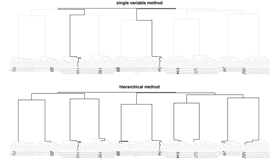
Figure 1: Dendrograms for a representative run of the “large blocks”-design with high SNR (SNR=8) and $\rho=0.85$. The active variables are labeled in black and the truly detected non-zero variables along the hierarchy are depicted in black.

For additional illustration, we show in Figure 1 the dendrograms (in gray) for a representative simulation run of the “large blocks”-design with $\rho=0.85$, for the single variable method and the hierarchical method with hclust clustering. The active variables are labeled in black and truly detected non-zero variables along the hierarchy are depicted in black. While the single variable method “only” detects 2 singletons, the hierarchical method detects the same 2 singletons and achieves 8 more MTDs (one of which has small cardinality 3 and hence is particularly informative). Figure 2 is analogous to Figure 1 for a simulation run of the “small blocks”-design with $\rho=0.8$. It shows that the hierarchical method improves the results of the single variable method (9 detected singletons) by additionally providing one MTD of cardinality 2 besides the same 9 singletons of the single variable method. Thus, we provide evidence of the fact that the hierarchical method has the powerful advantage of automatically going to the finer possible resolution, depending on signal-strength and correlation structure among the variables.

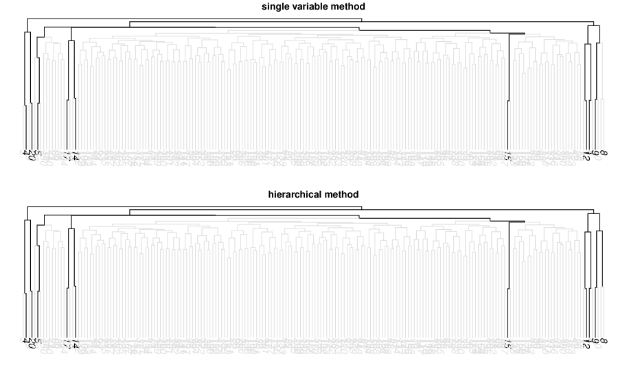
Figure 2: Dendrograms for a representative run of the “small blocks”-design with high SNR (SNR=8) and $\rho=0.80$. The active variables are labeled in black and the truly detected non-zero variables along the hierarchy are depicted in black.

Finally, we illustrate in Figure 3 the true positive (TPR) rates and false positive rates (FPR) of the Lasso, the single variable method and the hierarchical method with hclust clustering as points in the ROC space.

Figure 3: True positive rate (TPR) and false positive rate (FPR) for the Lasso (bullet), the single variable method (box), and the hierarchical method with hclust clustering (cross) for different scenarios as indicated in the header of the plots.

We note that, as expected from the philosophy of the single variable and hierarchical methods to control the FWER, there is a substantial difference between the FPR of the Lasso (0.15 to 0.18) and the FPR of the other 2 methods which is always less than 0.03 and equals 0 in most of the cases. For the “small blocks”-design, this improvement of the FPR has no negative impact on the TPR, while for the more difficult “large blocks”-design, a TPR comparable to that of the Lasso can only be achieved by the hierarchical method which significantly improves the TPR of the single variable method. It has to be remarked that the TPR and FPR are based on MTDs (regardless from their cardinality), hence some care is needed when comparing the TPR and FPR of the hierarchical with those of the other methods where only singleton detections are possible. For a detailed analysis we refer to Table 4.

In the Supplemental Material we present the same detailed analysis as in this section considering the same designs but with low $\mbox{SNR}=4$ signal to noise ratio.

4.4 Real data application: Motif Regression

We apply the three methods described in Section 4.1 to a real dataset about motif regression (Conlon et al.,, 2003) with $n=287$ and $p=195$, used in Meinshausen et al., (2009, Section 4.3). The single variable method identifies one single predictor variable as significant (controlling the familywise error rate at 5%). The same variable is found to be significant with the hierarchical method with hclust clustering, while the hierarchical method with canonical correlation clustering identifies as significant clusters, in the sense of Section 4.2.1, the singleton, which is the same single predictor as found by the other two methods, and a very big cluster of 165 variables. This is an interesting finding saying that besides the single predictor variable, there are presumably other motifs, in the large cluster, which play a relevant role. However, there is not enough information to determine which of the variables in the large cluster are significant as a single motif.

4.5 Conclusions from the empirical results

We have studied error rate control and performance of the three methods over 42 scenarios. The familywise error rate control was respected for all methods in 39 out of 42 scenarios, for 2 scenarios it is slightly non-respected by all methods (7 or 8 runs with at least a false selection out of 100). Considering Performance 1, we can see that the single variable method performs slightly better for settings where the correlation is not particularly high and the hierarchical methods perform better for settings with high correlation. If one looks at Performance 2, the disadvantage of the hierarchical methods in the “normal correlation” settings gets smaller (difference of 1.6 percent at most and 0.2 percent on average), while their advantage in the “high correlation” settings gets more substantial, with an average (over all scenarios) improvement of 5 percent when considering canonical correlation clustering and 7 percent when considering hclust clustering.

Taking a a more detailed and informative viewpoint in Section 4.3, the hierarchical method dominates the single variable method in terms of minimal true detections (MTDs), while both method detects a similar number of singletons (the hierarchical method being slightly preferable in this aspect, too). While both methods exhibit a good performance for the scenario generated with $\rho=0$, the clear superiority of the hierarchical method becomes apparent for increasing values of the correlations among the variables. The empirical findings supporting this statement are supported with additional results presented in the Supplemental Material.

Applying the hierarchical methods to a real dataset about motif regression (Conlon et al.,, 2003), we obtained an indication that there might be other potential motifs in a large cluster of size 165 which could play a significant role.

5 Robustness of the method with respect to failure of variable screening

The variable screening assumption (A2) seems far from necessary for controlling the FWER as described in Theorem 1. Table 4 provides empirical support for this fact.

5.1 A heuristic explanation

The following argument yields some explanation why the screening property is a too restrictive assumption. Let us assume that the screening property fails because the beta-min condition (5) fails to hold. We then expect rather different selected sets $\hat{S}^{(1)},\ldots,\hat{S}^{(B)}$, and the resulting p-values $p_{adj}^{C,(1)},\ldots,p_{adj}^{C,(B)}$ based on these selected sets are likely to be rather different as well (since $\hat{S}^{(b)}\not\supseteq S_{0}$ for most of the the $b$’s): many of them wouldn’t exhibit a small value and thus, when aggregating these p-values, the resulting aggregated p-value is likely to be non-small. For example, when aggregating with the sample median ($\gamma=1/2$ in Section 2.4), more than 50% of the p-values would need to be small such that the aggregated value would be small as well; and thus, the method only makes rejections if the single p-values $p_{adj}^{C,(1)},\ldots,p_{adj}^{C,(B)}$ are stable and a substantial fraction of them are small (and hence, we expect conservative behavior with respect to FWER control). We note that failure of (A2) due to a different reason than failure of the beta-min condition (5), such as ill-posed correlations among the variables, might lead to stable p-values where a large fraction of them are spuriously small: and in such a circumstance, the method might perform poorly with respect to controlling the FWER.

5.2 A mathematical argument based on zonal assumptions

We rigorously argue here that failure of the beta-min condition (5) still leads to control of the FWER, assuming alternative and weaker zonal assumptions (Bühlmann and Mandozzi,, 2014).

We partition the active set $S_{0}$ into sets with corresponding large and small regression coefficients, respectively:

$$S_{0}=S_{0,large}(a)\cup S_{0,small}(u),$$

$$S_{0,large}(a)=\{j;|\beta_{j}^{0}|>a\},\ \ S_{0,small}(u)=\{j;|\beta_{j}^{0}|\leq u\},$$

where $0<u<a$.

Consider the model $(\ref{mod1})$ with noise vector $\varepsilon\sim\mathcal{N}(0,\sigma^{2}I)$. It can be rewritten as

$$\mathbf{Y}=\mathbf{X}^{\hat{S}}\beta_{\hat{S}}^{0}+\mathbf{X}^{\hat{S}^{c}}\beta_{\hat{S}^{c}}^{0}+\varepsilon,$$

where $\hat{S}=\hat{S}(I_{1})\subseteq\{1\dots p\}$, $|\hat{S}|\leq|I_{2}|$ and $\mathbf{X}^{\hat{S}}$ the design sub-matrix of $\mathbf{X}$ with columns corresponding to $\hat{S}$, and $I_{1},\ I_{2}$ denote the two sub-samples such that $I_{1}\cup I_{2}=\{1,\ldots n\}$. Assume for the $|I_{2}|\times|\hat{S}|$ design sub-matrix $\mathbf{X}_{I_{2}}^{\hat{S}}$ of $\mathbf{X}$ with rows corresponding to $I_{2}$ and columns corresponding to $\hat{S}$:

$$\mbox{rank}((\mathbf{X}_{I_{2}}^{\hat{S}})^{T}\mathbf{X}_{I_{2}}^{\hat{S}})=|\hat{S}|.$$ (10)

Then define the following least squares estimates based on the sub-sample $I_{2}$ and using only the variables from $\hat{S}$:

$$\hat{\beta}_{I_{2}}^{\hat{S}}=\big{(}(\mathbf{X}_{I_{2}}^{\hat{S}})^{T}\mathbf{X}_{I_{2}}^{\hat{S}}\big{)}^{-1}(\mathbf{X}_{I_{2}}^{\hat{S}})^{T}Y_{I_{2}},$$

$$P_{I_{2}}^{\hat{S}}=\mathbf{X}_{I_{2}}^{\hat{S}}\big{(}(\mathbf{X}_{I_{2}}^{\hat{S}})^{T}\mathbf{X}_{I_{2}}^{\hat{S}}\big{)}^{-1}(\mathbf{X}_{I_{2}}^{\hat{S}})^{T},\ \ Q_{I_{2}}^{\hat{S}}=I_{I_{2}}-P_{I_{2}}^{\hat{S}},$$

$$\hat{Y}_{I_{2}}^{\hat{S}}=P_{I_{2}}^{\hat{S}}Y_{I_{2}}=\mathbf{X}_{I_{2}}^{\hat{S}}\hat{\beta}_{I_{2}}^{\hat{S}},\ \ \hat{\varepsilon}_{I_{2}}^{\hat{S}}=Q_{I_{2}}^{\hat{S}}Y_{I_{2}}=Y_{I_{2}}-\hat{Y}_{I_{2}}^{\hat{S}},$$

$$(\hat{\sigma}_{I_{2}}^{\hat{S}})^{2}=\frac{\|\hat{\varepsilon}_{I_{2}}^{\hat{S}}\|_{2}^{2}}{|I_{2}|-|\hat{S}|}.$$

Theorem 3.

Consider any selector $\hat{S}$ which is based on the sub-sample $I_{1}$ and satisfies (10). Then, for a $q\times|\hat{S}|$-matrix $A$,

$$\frac{(A\hat{\beta}_{I_{2}}^{\hat{S}}-A\beta_{\hat{S}}^{0})^{T}\big{(}A\big{(}\mathbf{X}_{I_{2}}^{\hat{S},T}\mathbf{X}_{I_{2}}^{\hat{S}}\big{)}^{-1}A^{T}\big{)}^{-1}(A\hat{\beta}_{I_{2}}^{\hat{S}}-A\beta_{\hat{S}}^{0})}{q(\hat{\sigma}_{I_{2}}^{\hat{S}})^{2}}\sim F_{q,|I_{2}|-|\hat{S}|}(\lambda_{\text{noncentral}})$$

is noncentral $F$-distributed with noncentrality parameter

$$\lambda_{\mbox{noncentral}}=\sum_{i=1}^{q}(\mbox{BIAS})_{i}^{2},$$

$$\mbox{BIAS}=\frac{1}{\sigma}\big{(}A\big{(}(\mathbf{X}_{I_{2}}^{\hat{S}})^{T}\mathbf{X}_{I_{2}}^{\hat{S}}\big{)}^{-1}A^{T}\big{)}^{-1/2}A\big{(}(\mathbf{X}_{I_{2}}^{\hat{S}})^{T}\mathbf{X}_{I_{2}}^{\hat{S}}\big{)}^{-1}(\mathbf{X}_{I_{2}}^{\hat{S}})^{T}\mathbf{X}_{I_{2}}^{\hat{S}^{c}}\beta_{\hat{S}^{c}}^{0}.$$

A proof is given in the Supplemental Material. Theorem 3 gives the distribution of the partial F-test statistic in the general case where a failure of screening is possible. The noncentrality parameter $\lambda_{\text{noncentral}}$, however, is unknown in practice. Clearly, if $\hat{S}\supseteq S_{0}$, then $\beta_{\hat{S}^{c}}^{0}=0$ and the noncentrality parameter $\lambda_{\text{noncentral}}=0$. Thus, if $\hat{S}$ is approximately correct for screening $S_{0}$, then $\lambda_{\text{noncentral}}\approx 0$.

In the following example we show that considering the Lasso as screening procedure and assuming zonal assumptions on the active variables, Theorem 3 implies asymptotically valid p-values when taking a partial F-test with central F-distribution (i.e, the noncentrality parameter is asymptotically negligible).

5.3 The Lasso as selector $\hat{S}$ and zonal assumptions for $\beta^{0}$

For the Lasso, assuming that the compatibility condition holds with compatibility constant $\phi^{2}_{0}>0$ (Bühlmann and van de Geer,, 2011, cf.(6.4)), with probability tending to one:

$$\|\hat{\beta}-\beta^{0}\|_{\infty}\leq\|\hat{\beta}-\beta^{0}\|_{1}\leq a(n,p,s_{0},\mathbf{X},\sigma):=C\sigma s_{0}\sqrt{\log(p)/n}/\phi^{2}_{0}$$

for some $C=C(\lambda)>0$ when choosing the regularization parameter $\lambda\asymp\sigma\sqrt{\log(p)/n}$ (Bühlmann and van de Geer,, 2011, Th6.1). Hence on an event with high probability, we have for this $a=a(n,p,s_{0},\mathbf{X},\sigma)$,

$$\hat{S}\supseteq S_{0,large}(a)$$

(Bühlmann and Mandozzi,, 2014) and using the partitioning of $S_{0}$ it follows that

$${\|\beta_{\hat{S}^{c}}^{0}\|}_{\infty}\leq u\mbox{ and }{\|\beta_{\hat{S}^{c}}^{0}\|}_{0}\leq s_{0,small}(u).$$

Assuming constants $C_{1},C_{2}$ and $C_{3}$ such that

$$\max_{j=1,\dots,p}(\mathbf{X}_{I_{2}}^{T}\mathbf{X}_{I_{2}})_{jj}\leq C_{1}|I_{2}|$$

$$\max_{j,k\in\hat{S}}|\big{(}\mathbf{X}_{I_{2}}^{\hat{S},T}\mathbf{X}_{I_{2}}^{\hat{S}}\big{)}^{-1}|_{jk}\leq C_{2}|I_{2}|^{-1}$$

$$\max_{j,k=1,\dots,q}|\big{(}A\big{(}\mathbf{X}_{I_{2}}^{\hat{S},T}\mathbf{X}_{I_{2}}^{\hat{S}}\big{)}^{-1}A^{T}\big{)}^{-1/2}|_{jk}\leq C_{3}|I_{2}|^{1/2}$$

$$\mbox{for each }q\times|\hat{S}|\mbox{-matrix }A\mbox{ with }q<|\hat{S}|,~{}A_{jj}\in\{0,1\}\mbox{ and }A_{jk}=0\mbox{ for }j\neq k.$$

it follows for the noncentrality parameter

$$\lambda_{noncentral} \leq q\max_{i=1,\dots,q}(\mbox{BIAS})_{i}^{2}$$

$$\leq q\big{(}\frac{1}{\sigma}C_{3}|I_{2}|^{1/2}|\hat{S}|C_{2}|I_{2}|^{-1}|\hat{S}|C_{1}|I_{2}|s_{0,small}(u)u\big{)}^{2}$$

$$\leq \Big{(}\frac{C_{1}C_{2}C_{3}}{\sigma}|\hat{S}|^{5/2}|I_{2}|^{1/2}s_{0,small}(u)u\Big{)}^{2}$$

Now, assuming a more restrictive sparse eigenvalue condition on the design $\mathbf{X}$ we have $|\hat{S}|\leq C_{4}s_{0}$ for some constant $0<C_{4}<\infty$ (Zhang and Huang,, 2008; van de Geer et al.,, 2011) and hence for some constant $D=D(C_{1},C_{2},C_{3},C_{4})$

$$\lambda_{noncentral} \leq \big{(}\frac{D}{\sigma}s_{0}^{5/2}s_{0,small}(u)\sqrt{n}u\big{)}^{2},$$

i.e. the noncentrality parameter is negligible for $u$ being at most of small order $o(n^{-1/2})$. Note that the inequality above is implicit in the value $u$ since it involves $s_{0,small}(u)$: of course, we can give the upper bound

$$\lambda_{noncentral} \leq \big{(}\frac{D}{\sigma}s_{0}^{7/2}\sqrt{n}u\big{)}^{2},$$

implying that $u=o(s_{0}^{-7/2}n^{-1/2})$ suffices to obtain asymptotic negligibility of the noncentrality parameter.

We conclude as follows. Assume that (10), (5.3) hold and that the design matrix satisfies a sparse eigenvalue condition with sparse eigenvalue bounded away from zero. Furthermore, replace the screening property in (A2) by zonal assumptions for the regression coefficients:

$$S_{0}=S_{0,large}(a)\cup S_{0,small}(u),\mbox{ with}$$

$$a=C\sigma s_{0}\sqrt{\log(p)/n}/\phi^{2}_{0}\mbox{ for }C>0\mbox{ sufficiently large,}$$

$$u=\tilde{C}\sigma s_{0}^{-5/2}s^{-1}_{0,small}(u)n^{-1/2}\mbox{ for }\tilde{C}>0\mbox{ sufficiently small.}$$

Then, when using the Lasso as selector $\hat{S}$, our hierarchical p-value method provides asymptotic strong error control of the familywise error rate.

6 Conclusions

We propose a method for testing whether (mainly) groups of correlated variables are significant for explaining a response in a high-dimensional linear model. In presence of highly correlated variables (or nearly collinear smaller groups of variables), as is very common in high-dimensional data, it seems indispensable to adopt such a kind of an approach going beyond multiple testing of individual regression coefficients. The groups of variables are ordered within a given hierarchy, for example a cluster tree, which allows for powerful multiple testing adjustment. It automatically determines a good resolution level distinguishing between small and large groups of variables: the former are significant if the signal of one or few individual variables in such a small group is strong and/or the variables are not too highly correlated; and a large group can be significant even if the signals of (many) individual variables in the group are weak and the variables exhibit high correlation among themselves. The minimal true detections (MTDs) measure the power to detect significant smallest groups of variables, and our method performs well in terms of MTDs and substantially better than the analogue of a single variable method.

Our procedure is based on repeated sample splitting which was empirically found to be “robust” and reliable for controlling type I errors. We present some theory proving strong control of the familywise error rate, and our assumptions allow for scenarios beyond the beta-min condition saying that all non-zero regression coefficients should be sufficiently large. We also provide empirical results for simulated and real data which complement the theoretical analysis.

Acknowledgments: We thank Nicolai Meinshausen and Patric Müller for interesting comments and discussions. Furthermore, we thank some anonymous reviewers for constructive and insightful comments.

7 Supplemental Materials

Supplemental Material for “Hierarchical Testing in the High-Dimensional Setting with Correlated Variables”:

An alternative bottom-up hierarchical adjustment. Variability of Performance 1 and Performance 2 in the simulations study. Variability of MTDs in Section 4.3. Extension of the considerations of Section 4.3 for low SNR. Proofs. (pdf file)

Supplemental material to Section 2

An alternative bottom-up hierarchical adjustment

The procedure described in Section 2 is based on a top-down hierarchical adjustment of the p-values $P_{h}^{C}=\max_{D\in\mathcal{T}:C\subseteq D}P^{C}$. Another possibility is the following bottom-up approach.

We begin with clustering as in Section 2.1 and screening as in Section 2.2. Then we take the p-values $p^{C,(b)}$ as in (2) and define

$$\overline{p}^{C,(b)}_{h}=\min\{\,2|\hat{S}^{(b)}|\min_{D\in\mathcal{T}:D\subseteq C}p^{C,(b)}\,,\,1\}.$$

Finally we define for $\gamma\in(0,1)$ the aggregated p-values

$$\overline{Q}_{h}^{C}(\gamma)=\min\big{\{}\,1~{},~{}q_{\gamma}\big{(}\big{\{}\overline{p}_{h}^{C,(b)}/\gamma;\,b=1,\dots,B\big{\}}\big{)}\big{\}}$$

and eliminate $\gamma$ taking

$$\overline{P}_{h}^{C}=\min\big{\{}\,1~{},~{}(1-\log\gamma_{\min})\inf_{\gamma\in(\gamma_{\min},1)}\overline{Q}_{h}^{C}(\gamma)\big{\}}.$$

The price one has to pay for minimizing among p-values of children clusters instead of maximizing among p-values of parents clusters is a factor $|C\cap\hat{S}^{(b)}|$ in the multiplicity adjustment.

Although none of the two methods theoretically dominates the other, simulations with some scenarios as in Section 4 have shown that the top-down method exhibits substantially higher power than the bottom-up method. Hence we put our focus on the top-down method.

Supplemental material to Section 4

Variability of Performance 1 and Performance 2 in the simulation study

To give some idea about the variability among the different simulation runs, we show in Figures 4 and 5 the Performance 1 and Performance 2 measures, respectively for all 100 runs of some of the scenarios.

Figure 4: The Performance 1 measure for all 100 runs for 2 different scenarios described in the header of the plots. Single variable method (filled small circle), the hierarchical method with canonical correlation clustering (empty square) and hclust clustering (triangle).

In Figure 4 we consider Performance 1 for two synthetic scenarios, one where the single variable method is favored and another where the hierarchical method is better. In Figure 5 we adopt the same approach for Performance 2 considering two scenarios based on semi-real datasets.

Figure 5: The Performance 2 measure for all 100 runs for 2 different scenarios described in the header of the plots. Single variable method (filled small circle), the hierarchical method with canonical correlation clustering (empty square) and hclus clustering (triangle).

Variability of MTDs in Section 4.3

We show in Figures 6 and 7 the number of MTDs for all simulation runs of the “small blocks”-design with $\mbox{SNR}=8$ and $\rho=0.7$ and $\rho=0.95$, respectively, and for the “large blocks”-design with $\mbox{SNR}=8$ and $\rho=0.4$ and $\rho=0.9$, respectively. For each of the 100 simulation runs and cardinalities from 1 to 20, the number of MTDs for the hierarchical method with hclus clustering is depicted in black while the number of MTDs for the single variable method is depicted in gray, for graphical convenience at the bottom of the y-axis (since the cardinality of the MTDs of the single variable method is always equal to 1).

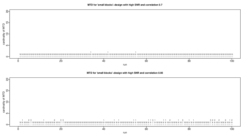
Figure 6: Number of MTDs for “small blocks”-design with high SNR (SNR=8) and $\rho=0.7$ resp. $\rho=0.95$. For each of the 100 simulation runs (x-axis) and every cardinality (y-axis), the number of MTDs for the hierarchical method with hclus clustering (in black) and for the single variable method (in gray, for graphical convenience at the bottom of the y-axis).

Figure 7: Number of MTDs for “large blocks”-design with high SNR (SNR=8) and $\rho=0.7$ resp. $\rho=0.9$. For each of the 100 simulation runs (x-axis) and every cardinality (y-axis), the number of MTDs for the hierarchical method with hclus clustering (in black) and for the single variable method (in gray, for graphical convenience at the bottom of the y-axis).

Extension of the considerations of Section 4.3 for low SNR

We present here the same detailed analysis as in Section 4.3 for the signal to noise ratio $\mbox{SNR}=4$. The empirical results presented below show that the power of all considered methods is significantly affected by the change of SNR (e.g. for the “large blocks”-design with $\rho\geq 0.7$ detecting at least one singleton is difficult when $\mbox{SNR}=4$), but they also confirm the superiority of the hierarchical in comparison to the single variable methods reported in the main paper in Section 4.3.

Table 5 reports some average results over 100 simulation runs. As for the case in the main paper with high SNR, the number of singleton detections are again similar for all methods. The large number of MTDs with cardinality 2 in the “small blocks”-design emphasizes the powerful advantage of automatically going to the finer possible resolution with the hierarchical method.

		FWER			# MTD			# MTD for given cardinality
$\rho$	$\delta$							$|\cdot|=1$			$|\cdot|=2$		$3\leq|\cdot|\leq 10$		$11\leq|\cdot|\leq 20$
		S	C	H	S	C	H	S	C	H	C	H	C	H	C	H
“small blocks”-design with low SNR
0	0.28	0	0	0	8.78	8.85	8.79	8.78	8.72	8.49	0	0.03	0	0.09	0	0.07
0.4	0.18	0	0	0	8.74	9.11	8.82	8.74	8.83	8.47	0.26	0.05	0.02	0.08	0	0.01
0.7	0.45	0	0	0	4.80	6.89	7.02	4.80	5.26	4.86	1.41	1.21	0	0.56	0.19	0
0.8	0.49	0	0	0	4.74	7.13	7.41	4.74	4.95	4.78	1.99	2.00	0.02	0.55	0.16	0.04
0.85	0.38	0.03	0.03	0.03	6.03	7.84	8.00	6.03	6.39	6.10	1.41	1.70	0.04	0.20	0	0
0.9	0.53	0.05	0.05	0.07	4.31	7.07	7.47	4.31	4.63	4.67	2.22	2.23	0.06	0.56	0.16	0
0.95	0.98	0.33	0.36	0.42	1.29	3.83	4.82	1.29	1.48	1.28	1.95	2.02	0	1.08	0.26	0
0.99	0.94	0.46	0.60	0.54	3.96	6.47	6.66	3.96	4.06	3.63	2.26	2.28	0.15	0.39	0	0.13
“large blocks”-design with low SNR
0	0.24	0	0	0	8.18	8.20	8.23	8.18	8.03	7.86	0	0.18	0	0.25	0	0.09
0.4	0.35	0	0	0	4.51	5.06	6.90	4.51	4.53	4.26	0.01	0.14	0.06	0.46	0.24	1.31
0.7	0.76	0	0	0	0.28	2.84	4.69	0.28	0.30	0.27	0	0.06	0.11	0.26	1.88	2.36
0.8	0.72	0	0	0	0.58	4.93	6.48	0.58	0.63	0.60	0	0.07	0.35	0.66	3.67	3.83
0.85	0.82	0	0	0.01	0.48	5.53	6.42	0.48	0.48	0.46	0	0.04	0.44	0.54	4.40	4.30
0.9	0.99	0	0	0	0.08	3.6	4.61	0.08	0.10	0.08	0	0	0.16	0.17	2.77	2.77
0.95	1.00	0	0.23	0.15	0.10	6.98	7.25	0.10	0.10	0.10	0.01	0.03	0.27	0.87	6.40	5.86
0.99	1.00	0.93	1.00	1.00	1.60	5.00	5.10	1.60	1.60	1.60	0	0.24	1.49	2.21	1.91	1.05

Table 5: Results of the simulation with the “large blocks”- and “small blocks” -design with low SNR (SNR=4) for different correlations. $\rho$ is the correlation in the design, $\delta$ the relative frequency of screenings with $\hat{S}\not\supset S_{0}$, MTD denotes “minimal true detections”, “$2\leq|\cdot|\leq 5$” indicates that MTD of cardinality between 2 and 5 are considered, S, C and H represent the “single variable” resp. ”canonical correlation clustering“ and “hierarchical with hclus clustering” method.

To better illustrate what happens in a typical simulation run, we show in Figure 8 the dendrograms for a representative simulation run of the “large blocks”-design with $\rho=0.85$ (here with $\mbox{SNR}=4$), for the single variable method and the hierarchical method with hclus clustering. The active variables are labeled in black and the truly detected non-zero variables along the hierarchy are depicted in black. While the single variable method “only” detects one singleton, the hierarchical method detects the same singleton and achieves 8 more MTDs.

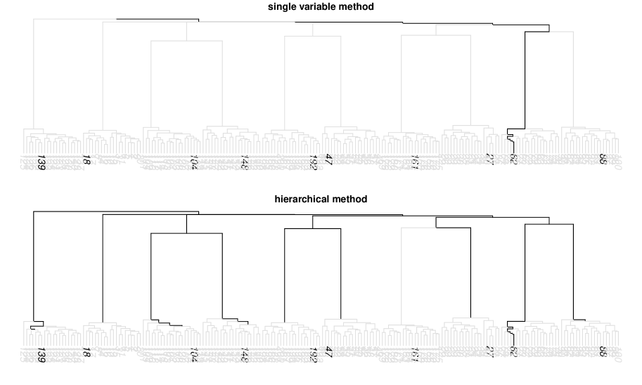
Figure 8: Dendrograms for a representative run of the “large blocks”-design with low SNR (SNR=4) and $\rho=0.85$. The active variables are labeled in black and the truly detected non-zero variables along the hierarchy are depicted in black.

Figure 9 is the analogous of Figure 8 in the main paper for a typical run of the “small blocks”-design with $\rho=0.8$. It shows that the hierarchical method improves the results of the single variable method (which detects 5 singletons) providing 3 more MTDs of cardinality 2.

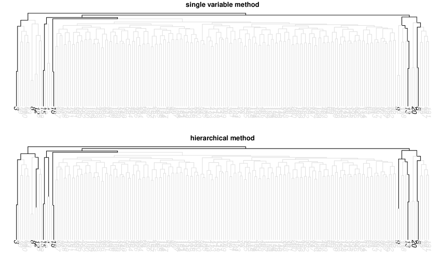
Figure 9: Dendrograms for a representative run of the “small blocks”-design with low SNR (SNR=4) and $\rho=0.80$. The active variables are labeled in black and the truly detected non-zero variables along the hierarchy are depicted in black.

In Figures 10 and 11 and we show the number of MTDs for all 100 simulation runs of the “small blocks”-design with $\mbox{SNR}=4$ and $\rho=0.7$ and $\rho=0.9$, respectively. and for the “large blocks”-design with $\mbox{SNR}=4$ and $\rho=0.4$ and $\rho=0.9$, respectively. For each simulation run and cardinalities from 1 to 20, the number of MTDs for the hierarchical method with hclus clustering is depicted in black while the number of MTDs for the single variable method is depicted in gray, for graphical convenience at the bottom of the y-axis (since the cardinality of MTDs of the single variable method is always equal to 1).

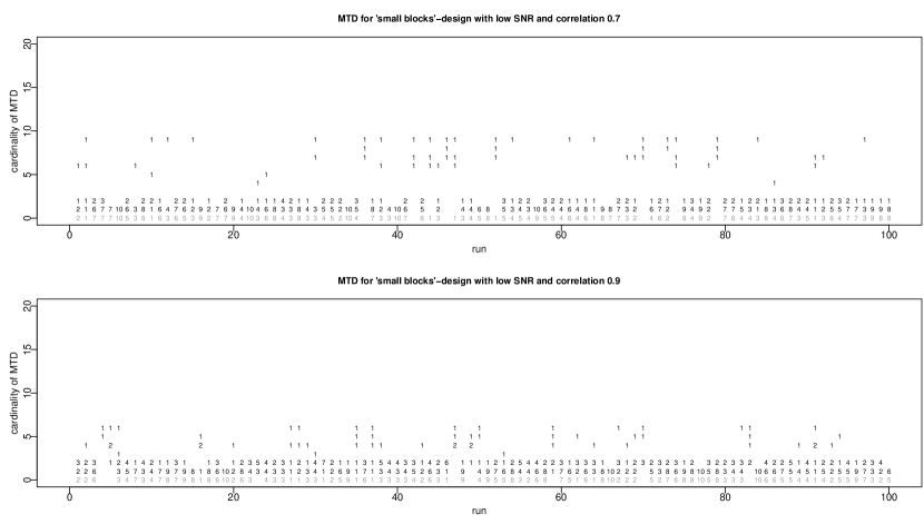
Figure 10: Number of MTDs for “small blocks”-design with high SNR (SNR=4) and $\rho=0.7$ resp. $\rho=0.9$. For each of the 100 simulation runs (x-axis) and every cardinality (y-axis), the number of MTDs for the hierarchical method with hclus clustering (in black) and for the single variable method (in gray, for graphical convenience at the bottom of the y-axis).

Figure 11: Number of MTDs for “large blocks”-design with high SNR (SNR=4) and $\rho=0.7$ resp. $\rho=0.9$. For each of the 100 simulation runs (x-axis) and every cardinality (y-axis), the number of MTDs for the hierarchical method with hclus clustering (in black) and for the single variable method (in gray, for graphical convenience at the bottom of the y-axis).

Finally, we illustrate in Figure 12 the true positive (TPR) rates and false positive rates (FPR) of the Lasso, the single variable and the hierarchical method with hclus clustering as points in the ROC space.

Figure 12: True positive rate (TPR) and false positive rate (FPR) for the Lasso (bullet), the single variable method (box), and the hierarchical method with hclust clustering (cross) for different scenarios as indicated in the header of the plots.

Comparing Figure 12 with Figure 3 in the main paper, we see that the negative impact of low SNR is more striking on the TPR then on the FPR which remains very similar. Regarding a comparison of the methods, the same conclusions as for high $\mbox{SNR}=8$ can be drawn: the single variable and hierarchical method do much better than the Lasso in terms of FPR. The price one has to pay for the higher reliability is a lower TPR and the hierarchical method improves the TPR of the single variable method to the level of the Lasso (when considering MTDs).

Proofs

Proof of Theorem 1

Our proof is following ideas from the proofs of Theorem 3.1-3.2 in Meinshausen et al., (2009) and the proof Theorem 1 in Meinshausen, (2008).

Proof of first assertion of Theorem 1.
First note that

$$\mathbb{P}(\mathcal{T}^{\gamma}_{rej}\cap\mathcal{T}_{0}\neq\emptyset) = \mathbb{P}(\exists C\in\mathcal{T}_{0}\,:\,Q^{C}_{h}(\gamma)\leq\alpha)$$

$$= \mathbb{P}(\exists C\in\tilde{\mathcal{T}}_{0}\,:\,Q^{C}_{h}(\gamma)\leq\alpha)$$

where $\tilde{\mathcal{T}}_{0}$ is the set of all clusters which fulfill the null hypothesis and are maximal in the sense that

$$\tilde{\mathcal{T}}_{0}:=\{C\in\mathcal{T}_{0}\,:\,\nexists D\in\mathcal{T}_{0}\mbox{ with }C\subset D\}.$$

This holds, since a direct consequence of the definition of the hierarchically adjusted p-values $Q^{C}_{h}(\cdot)$ is that $Q^{C^{\prime}}_{h}(\gamma)\leq Q^{C}_{h}(\gamma)\mbox{ for }C\subset C^{\prime}$ and hence an error committed on a cluster $C\in\mathcal{T}_{0}\backslash\tilde{\mathcal{T}}_{0}$ implies an error in a set $C^{\prime}\in\tilde{\mathcal{T}}_{0}$, with $C\subset C^{\prime}$. Moreover, since $Q^{C}_{h}(\gamma)\geq Q^{C}(\gamma)$,

$$\mathbb{P}(\exists C\in\tilde{\mathcal{T}}_{0}\,:\,Q^{C}_{h}(\gamma)\leq\alpha)\leq\mathbb{P}(\exists C\in\tilde{\mathcal{T}}_{0}\,:\,Q^{C}(\gamma)\leq\alpha)=\mathbb{P}(\min_{C\in\tilde{\mathcal{T}}_{0}}Q^{C}(\gamma)\leq\alpha).$$

Hence it remains to show that

$$\mathbb{P}(\min_{C\in\tilde{\mathcal{T}}_{0}}Q^{C}(\gamma)\leq\alpha)\leq\alpha.$$

We consider the event

$$\mathcal{A}=\{\,\hat{S}^{(b)}\supseteq S_{0},\forall\,b=1\dots B\,\}$$

where all screenings are satisfied. Because of the $\delta$-screening assumption it holds

$$\\ P(\mathcal{A})\geq(1-\delta)^{B}.$$

In the following we omit the function $\min\{1,\cdot\}$ from the definition of $Q^{C}(\gamma)$ in order to simplify the notation (this is possible since the level $\alpha$ is smaller than 1). Define for $u\in(0,1)$ the function

$$\pi^{C}(u):=\frac{1}{B}\sum_{b=1}^{B}1\{p^{C,(b)}_{adj}\leq u\}.$$

Then it holds

$$Q^{C}(\gamma)\leq\alpha \Longleftrightarrow q_{\gamma}(\{p^{C,(b)}_{adj}/\gamma;\,b=1,\dots,B\})\leq\alpha$$

$$\Longleftrightarrow q_{\gamma}(\{p^{C,(b)}_{adj};\,b=1,\dots,B\})\leq\alpha\gamma$$

$$\Longleftrightarrow \sum_{b=1}^{B}1\{p^{C,(b)}_{adj}\leq\alpha\gamma\}\geq B\gamma$$

$$\Longleftrightarrow \pi^{C}(\alpha\gamma)\geq\gamma.$$

Thus

$$\mathbb{P}(\min_{C\in\tilde{\mathcal{T}}_{0}}Q^{C}(\gamma)\leq\alpha) \leq \sum_{C\in\tilde{\mathcal{T}}_{0}}\mathbb{E}(1\{Q^{C}(\gamma)\leq\alpha\})$$

$$= \sum_{C\in\tilde{\mathcal{T}}_{0}}\mathbb{E}(1\{\pi^{C}(\alpha\gamma)\geq\gamma\})$$

$$\leq \frac{1}{\gamma}\sum_{C\in\tilde{\mathcal{T}}_{0}}\mathbb{E}(\pi^{C}(\alpha\gamma)),$$

where for the last inequality a Markov inequality was used. Now, using the definition of $\pi^{C}(\cdot)$,

$$\frac{1}{\gamma}\sum_{C\in\tilde{\mathcal{T}}_{0}}\mathbb{E}(\pi^{C}(\alpha\gamma)) = \frac{1}{\gamma}\sum_{C\in\tilde{\mathcal{T}}_{0}}\mathbb{E}(\frac{1}{B}\sum_{b=1}^{B}1\{p^{C,(b)}_{adj}\leq\alpha\gamma\})$$

$$= \frac{1}{\gamma}\frac{1}{B}\sum_{b=1}^{B}\sum_{C\in\tilde{\mathcal{T}}_{0}}\mathbb{E}(1\{p^{C,(b)}_{adj}\leq\alpha\gamma\})$$

$$= \frac{1}{\gamma}\frac{1}{B}\sum_{b=1}^{B}\sum_{C\in\tilde{\mathcal{T}}_{0},\,\hat{S}^{(b)}\cap C\neq\emptyset}\mathbb{E}(1\{p^{C,(b)}_{adj}\leq\alpha\gamma\})$$

where the last equality holds since $p^{C,(b)}_{adj}=1$ if $\hat{S}^{(b)}\cap C=\emptyset$. Now, for $C$ such that $\hat{S}^{(b)}\cap C\neq\emptyset$ and on $\mathcal{A}$

$$\mathbb{E}(1\{p^{C,(b)}_{adj}\leq\alpha\gamma\}) = \mathbb{P}(p^{C,(b)}_{adj}\leq\alpha\gamma)$$

$$= \mathbb{P}\Big{(}p^{C,(b)}\frac{|\hat{S}^{(b)}|}{|C\cap\hat{S}^{(b)}|}\leq\alpha\gamma\Big{)}$$

$$= \mathbb{P}\Big{(}p^{C,(b)}\leq\alpha\gamma\frac{|C\cap\hat{S}^{(b)}|}{|\hat{S}^{(b)}|}\Big{)}$$

$$\leq \alpha\gamma\frac{|C\cap\hat{S}^{(b)}|}{|\hat{S}^{(b)}|}.$$

This is a consequence of the uniform distribution of the p-values $p^{C\cap\hat{S}^{(b)}}$ given $S\subseteq\hat{S}^{(b)}$ and the sample split $\{1,\dots,n\}=N_{in}^{(b)}\sqcup N_{out}^{(b)}$. We can hence conclude that on $\mathcal{A}$

$$\mathbb{P}(\min_{C\in\tilde{\mathcal{T}}_{0}}Q^{C}(\gamma)\leq\alpha) \leq \frac{1}{\gamma}\frac{1}{B}\sum_{b=1}^{B}\sum_{C\in\tilde{\mathcal{T}}_{0},\,\hat{S}^{(b)}\cap C\neq\emptyset}\alpha\gamma\frac{|C\cap\hat{S}^{(b)}|}{|\hat{S}^{(b)}|}$$

$$= \alpha\frac{1}{B}\sum_{b=1}^{B}\frac{1}{|\hat{S}^{(b)}|}\sum_{C\in\tilde{\mathcal{T}}_{0},\,\hat{S}^{(b)}\cap C\neq\emptyset}|C\cap\hat{S}^{(b)}|$$

$$\leq \alpha\frac{1}{B}\sum_{b=1}^{B}1\leq\alpha,$$

since by definition the sets in $\tilde{\mathcal{T}}_{0}$ are disjoint and hence

$$\sum_{C\in\tilde{\mathcal{T}}_{0},\,\hat{S}^{(b)}\cap C\neq\emptyset}|C\cap\hat{S}^{(b)}|\leq|\hat{S}^{(b)}|.$$

Finally we have

$$\mathbb{P}(\min_{C\in\tilde{\mathcal{T}}_{0}}Q^{C}(\gamma)\leq\alpha)=$$

$$= \mathbb{P}(\min_{C\in\tilde{\mathcal{T}}_{0}}Q^{C}(\gamma)\leq\alpha\,|\,\mathcal{A})\,P(\mathcal{A})+\mathbb{P}(\min_{C\in\tilde{\mathcal{T}}_{0}}Q^{C}(\gamma)\leq\alpha\,|\,\mathcal{A}^{c})\,P(\mathcal{A}^{c})$$

$$\leq \alpha+1-(1-\delta)^{B}$$

Proof of second assertion of Theorem 1.
We show that

$$\mathbb{P}(\exists C\in\mathcal{T}_{0}\,:\,P^{C}_{h}\leq\alpha)\leq\alpha.$$

Defining $\tilde{\mathcal{T}}_{0}$ as in the proof of Theorem 1 and using similar arguments as there we obtain

$$\mathbb{P}(\exists C\in\mathcal{T}_{0}\,:\,P^{C}_{h}\leq\alpha)=\mathbb{P}(\exists C\in\tilde{\mathcal{T}}_{0}\,:\,P^{C}_{h}\leq\alpha)\leq\mathbb{P}(\exists C\in\tilde{\mathcal{T}}_{0}\,:\,P^{C}\leq\alpha).$$

As in the proof of Theorem 1 we consider the event

$$\mathcal{A}=\{\,\hat{S}^{b}\supseteq S_{0},\forall\,b=1\dots B\,\}$$

with $P(\mathcal{A})\geq(1-\delta)^{B}$. The uniform distribution of the p-values $p_{\mathrm{partial\>F-test}}^{C\cap\hat{S}^{(b)}}$ given $S\subseteq\hat{S}^{(b)}$ and the sample split $\{1,\dots,n\}=N_{in}^{(b)}\sqcup N_{out}^{(b)}$, together with the fact that sets in $\hat{S}^{(b)}$ are disjoint, provides on $\mathcal{A}$

$$\mathbb{E}\Big{(}\frac{1\{p^{C,(b)}\leq\alpha\gamma\}}{\gamma}\Big{)}=\frac{1}{\gamma}\mathbb{P}(p^{C,(b)}\leq\alpha\gamma)\leq\alpha.$$

Moreover, on $\mathcal{A}$

$$\mathbb{E}\Big{(}\max_{C\in\tilde{\mathcal{T}}_{0}}\frac{1\{p^{C,(b)}_{adj}\leq\alpha\gamma\}}{\gamma}\Big{)} \leq \mathbb{E}\Big{(}\sum_{C\in\tilde{\mathcal{T}}_{0}}\frac{1\{p^{C,(b)}_{adj}\leq\alpha\gamma\}}{\gamma}\Big{)}$$

$$\leq \mathbb{E}\Big{(}\sum_{C\in\tilde{\mathcal{T}}_{0},\,\hat{S}^{(b)}\cap C\neq\emptyset}\frac{1\{p^{C,(b)}_{adj}\leq\alpha\gamma\}}{\gamma}\Big{)}$$

$$= \frac{1}{\gamma}\sum_{C\in\tilde{\mathcal{T}}_{0},\,\hat{S}^{(b)}\cap C\neq\emptyset}\mathbb{P}(1\{p^{C,(b)}_{adj}\leq\alpha\gamma\})$$

$$\leq \frac{1}{\gamma}\sum_{C\in\tilde{\mathcal{T}}_{0},\,\hat{S}^{(b)}\cap C\neq\emptyset}\mathbb{P}\Big{(}p^{C,(b)}\frac{|\hat{S}^{(b)}|}{|C\cap\hat{S}^{(b)}|}\leq\alpha\gamma\Big{)}$$

$$\leq \frac{1}{\gamma}\sum_{C\in\tilde{\mathcal{T}}_{0},\,\hat{S}^{(b)}\cap C\neq\emptyset}\frac{|C\cap\hat{S}^{(b)}|}{|\hat{S}^{(b)}|}\alpha\gamma\leq\alpha$$

For a random variable $U$ taking values in $[0,1]$,

$$\sup_{\gamma\in(\gamma_{\min},1)}\frac{1\{U\leq\alpha\gamma\}}{\gamma}=\left\{\begin{array}[]{ll}0,&U\geq\alpha\\ \alpha/U,&\alpha\gamma_{\min}\leq U<\alpha\\ 1/\gamma_{\min},&U\leq\alpha\gamma_{\min}.\\ \end{array}\right.$$

and if $U$ has an uniform distribution on $[0,1]$

$$\mathbb{E}\Big{(}\sup_{\gamma\in(\gamma_{\min},1)}\frac{1\{U\leq\alpha\gamma\}}{\gamma}\Big{)} = \int_{0}^{\alpha\gamma_{\min}}\gamma_{\min}^{-1}dx+\int_{\alpha\gamma_{\min}}^{\alpha}\alpha x^{-1}dx$$

$$= \gamma_{\min}^{-1}x\big{|}_{x=0}^{x=\alpha\gamma_{\min}}+\alpha\log x\big{|}_{x=\alpha\gamma_{\min}}^{x=\alpha}$$

$$= \alpha+\alpha(\log\alpha-\log(\alpha\gamma_{\min}))$$

$$= \alpha\big{(}1-\log\frac{\alpha}{\alpha\gamma_{\min}}\big{)}$$

$$= \alpha(1-\log\gamma_{\min}).$$

We apply this using as $U$ the uniform distributed $p_{\mathrm{partial\>F-test}}^{C\cap\hat{S}^{(b)}}$ and obtain that on $\mathcal{A}$

$$\mathbb{E}\Big{(}\sup_{\gamma\in(\gamma_{\min},1)}\frac{1\{p^{C,(b)}\leq\alpha\gamma\}}{\gamma}\Big{)}\leq\alpha(1-\log\gamma_{\min}),$$

and similarly as above

$$\sum_{C\in\tilde{\mathcal{T}}_{0}}\mathbb{E}\Big{(}\sup_{\gamma\in(\gamma_{\min},1)}\frac{1\{p^{C,(b)}_{adj}\leq\alpha\gamma\}}{\gamma}\Big{)}\leq\alpha(1-\log\gamma_{\min}).$$

We can now consider the average over all random splits

$$\sum_{C\in\tilde{\mathcal{T}}_{0}}\mathbb{E}\Big{(}\sup_{\gamma\in(\gamma_{\min},1)}\frac{(1/B)\sum_{b=1}^{B}1\{p^{C,(b)}_{adj}\leq\alpha\gamma\}}{\gamma}\Big{)}\leq\alpha(1-\log\gamma_{\min})$$

and defining $\pi^{C}(\cdot)$ as in the proof of Theorem 1 and using a Markov inequality

$$\sum_{C\in\tilde{\mathcal{T}}_{0}}\mathbb{E}(\sup_{\gamma\in(\gamma_{\min},1)}1\{\pi^{C}(\alpha\gamma)\geq\gamma\})\leq\alpha(1-\log\gamma_{\min}).$$

We use now the fact, that the events $\{Q^{C}(\gamma)\leq\alpha\}$ and $\{\pi^{C}(\alpha\gamma)\geq\gamma\}$ are equivalent and deduce that on $\mathcal{A}$

$$\sum_{C\in\tilde{\mathcal{T}}_{0}}\mathbb{P}(\inf_{\gamma\in(\gamma_{\min},1)}Q^{C}(\gamma)\leq\alpha) \leq \alpha(1-\log\gamma_{\min}),$$

therefore on $\mathcal{A}$

$$\mathbb{P}(\exists C\in\tilde{\mathcal{T}}_{0}\,:\,P^{C}\leq\alpha) = \mathbb{P}(\min_{C\in\tilde{\mathcal{T}}_{0}}P^{C}\leq\alpha)$$

$$\leq \sum_{C\in\tilde{\mathcal{T}}_{0}}\mathbb{P}(P^{C}\leq\alpha)$$

$$\leq \sum_{C\in\tilde{\mathcal{T}}_{0}}\mathbb{P}(\inf_{\gamma\in(\gamma_{\min},1)}Q^{C}(\gamma)(1-\log\gamma_{\min})\leq\alpha)$$

$$\leq \alpha.$$

Finally

$$\mathbb{P}(\exists C\in\tilde{\mathcal{T}}_{0}\,:\,P^{C}\leq\alpha)=$$

$$= \mathbb{P}(\exists C\in\tilde{\mathcal{T}}_{0}\,:\,P^{C}\leq\alpha\,|\,\mathcal{A})\,P(\mathcal{A})+\mathbb{P}(\exists C\in\tilde{\mathcal{T}}_{0}\,:\,P^{C}\leq\alpha\,|\,\mathcal{A}^{c})\,P(\mathcal{A}^{c})$$

$$\leq \alpha+1-(1-\delta)^{B}$$

and the proof is concluded.

Proof of Theorem 2

As the only change to be considered with respect to Theorem 1 is the Shaffer multiplicity adjustment (7), it suffices to show that

$$\sum_{C\in\tilde{\mathcal{T}}_{0},\,\hat{S}^{(b)}\cap C\neq\emptyset}|C|^{\hat{S}^{(b)}}_{e\!f\!f}\leq|\hat{S}^{(b)}|.$$

It holds

$$\sum_{C\in\tilde{\mathcal{T}}_{0},\,\hat{S}^{(b)}\cap C\neq\emptyset}|C|^{\hat{S}^{(b)}}_{e\!f\!f}=\sum_{C\in\tilde{\mathcal{T}}_{0},\,\hat{S}^{(b)}\cap C\neq\emptyset}\Big{(}|C\cap\hat{S}^{(b)}|+$$

$$+|\mbox{si}(C)\cap\hat{S}^{(b)}|\,1\{\nexists E\in\mbox{ch}(\mbox{si}(C))\mbox{ s.t. }E\cap\hat{S}^{(b)}\neq\emptyset\}\Big{)}.$$

As noted in the proof of Theorem 1 the sets in $\tilde{\mathcal{T}}_{0}$ are disjoint. Moreover for any cluster $D\in\tilde{\mathcal{T}}_{0}$ with $\mbox{si}(D)\neq\emptyset$, $H_{0,\mbox{si}(D)}$ is false, otherwise because of the assumption that $\mathcal{T}$ is binary $H_{0,\mbox{pa}(D)}$ would also be true, leading to a contradiction to $D\in\tilde{\mathcal{T}}_{0}$. Consider now two sets $C,D\in\tilde{\mathcal{T}}_{0}$ with $\hat{S}^{(b)}\cap C\neq\emptyset$ and $\hat{S}^{(b)}\cap D\neq\emptyset$, since $H_{0,C}$ is true and $H_{0,\mbox{si}(D)}$ is false it must be $\mbox{si}(D)\not\subset C$. On the other hand if $C\subset\mbox{si}(D)$ then the term $|\mbox{si}(D)\cap\hat{S}^{(b)}|$ wouldn’t be considered in the sum, hence only disjoint $C$ and $\mbox{si}(D)$ are considered in the sum. Finally, suppose that for two sets $C,D\in\tilde{\mathcal{T}}_{0}$ with $\hat{S}^{(b)}\cap C\neq\emptyset$ and $\hat{S}^{(b)}\cap D\neq\emptyset$ it is $\mbox{si}(C)\subset\mbox{si}(D)$. Then if $|\mbox{si}(D)\cap\hat{S}^{(b)}|$ is considered in the sum it must be $\mbox{si}(C)\cap\hat{S}^{(b)}=\emptyset$. Putting all this together we conclude that all sets giving nontrivial contributions to the sum are disjoint.

Proof of Theorem 3

In order to prove Theorem 3 we introduce four Lemmas.

Lemma 1.

$$\big{(}\hat{\beta}_{I_{2}}^{\hat{S}}-\beta_{\hat{S}}^{0}\big{)}\sim\mathcal{N}\Big{(}\big{(}\mathbf{X}_{I_{2}}^{\hat{S},T}\mathbf{X}_{I_{2}}^{\hat{S}}\big{)}^{-1}\mathbf{X}_{I_{2}}^{\hat{S},T}\mathbf{X}_{I_{2}}^{\hat{S}^{c}}\beta_{\hat{S}^{c}}^{0},\sigma^{2}\big{(}\mathbf{X}_{I_{2}}^{\hat{S},T}\mathbf{X}_{I_{2}}^{\hat{S}}\big{)}^{-1}\Big{)}$$

Proof.

By definition

$$\hat{\beta}_{I_{2}}^{\hat{S}} = \big{(}\mathbf{X}_{I_{2}}^{\hat{S},T}\mathbf{X}_{I_{2}}^{\hat{S}}\big{)}^{-1}\mathbf{X}_{I_{2}}^{\hat{S},T}Y_{I_{2}}=\big{(}\mathbf{X}_{I_{2}}^{\hat{S},T}\mathbf{X}_{I_{2}}^{\hat{S}}\big{)}^{-1}\mathbf{X}_{I_{2}}^{\hat{S},T}\big{(}\mathbf{X}_{I_{2}}^{\hat{S}}\beta_{\hat{S}}^{0}+\mathbf{X}_{I_{2}}^{\hat{S}^{c}}\beta_{\hat{S}^{c}}^{0}+\varepsilon_{I_{2}}\big{)}$$

$$= \beta_{\hat{S}}^{0}+\big{(}\mathbf{X}_{I_{2}}^{\hat{S},T}\mathbf{X}_{I_{2}}^{\hat{S}}\big{)}^{-1}\mathbf{X}_{I_{2}}^{\hat{S},T}\mathbf{X}_{I_{2}}^{\hat{S}^{c}}\beta_{\hat{S}^{c}}^{0}+\big{(}\mathbf{X}_{I_{2}}^{\hat{S},T}\mathbf{X}_{I_{2}}^{\hat{S}}\big{)}^{-1}\mathbf{X}_{I_{2}}^{\hat{S},T}\varepsilon_{I_{2}}$$

and $\hat{\beta}_{I_{2}}^{\hat{S}}$ is as linear transformation of a normal distributed random variable also normal distributed. From the formula above its is easy to see that the expected value $\big{(}\hat{\beta}_{I_{2}}^{\hat{S}}-\beta_{\hat{S}}^{0}\big{)}$ is $\big{(}\mathbf{X}_{I_{2}}^{\hat{S},T}\mathbf{X}_{I_{2}}^{\hat{S}}\big{)}^{-1}\mathbf{X}_{I_{2}}^{\hat{S},T}\mathbf{X}_{I_{2}}^{\hat{S}^{c}}\beta_{\hat{S}^{c}}^{0}$. For the covariance we can calculate

$$\mbox{Cov}\big{(}\hat{\beta}_{I_{2}}^{\hat{S}}-\beta_{\hat{S}}^{0}\big{)} = \mbox{Cov}\big{(}\big{(}\mathbf{X}_{I_{2}}^{\hat{S},T}\mathbf{X}_{I_{2}}^{\hat{S}}\big{)}^{-1}\mathbf{X}_{I_{2}}^{\hat{S},T}\mathbf{X}_{I_{2}}^{\hat{S}^{c}}\beta_{\hat{S}^{c}}^{0}+\big{(}\mathbf{X}_{I_{2}}^{\hat{S},T}\mathbf{X}_{I_{2}}^{\hat{S}}\big{)}^{-1}\mathbf{X}_{I_{2}}^{\hat{S},T}\varepsilon_{I_{2}}\big{)}$$

$$= \big{(}\mathbf{X}_{I_{2}}^{\hat{S},T}\mathbf{X}_{I_{2}}^{\hat{S}}\big{)}^{-1}\mathbf{X}_{I_{2}}^{\hat{S},T}\mbox{Cov}(\varepsilon_{I_{2}})\mathbf{X}_{I_{2}}^{\hat{S}}\big{(}\mathbf{X}_{I_{2}}^{\hat{S},T}\mathbf{X}_{I_{2}}^{\hat{S}}\big{)}^{-1}$$

$$= \sigma^{2}\big{(}\mathbf{X}_{I_{2}}^{\hat{S},T}\mathbf{X}_{I_{2}}^{\hat{S}}\big{)}^{-1}$$

∎

Lemma 2.

$P_{I_{2}}^{\hat{S}}$ resp. $Q_{I_{2}}^{\hat{S}}$ is an orthogonal projection of $\mathbb{R}^{|I_{2}|}$ in $\mathbb{R}^{|\hat{S}|}$ resp. $\mathbb{R}^{|I_{2}|-|\hat{S}|}$.

Proof.

It follows from the definition of $P_{I_{2}}^{\hat{S}}$ and $Q_{I_{2}}^{\hat{S}}$, that they satisfy the equation $X^{T}=X=X^{2}$. Moreover

$$\mbox{tr}(P_{I_{2}}^{\hat{S}}) = \mbox{tr}(\mathbf{X}_{I_{2}}^{\hat{S}}\big{(}\mathbf{X}_{I_{2}}^{\hat{S},T}\mathbf{X}_{I_{2}}^{\hat{S}}\big{)}^{-1}\mathbf{X}_{I_{2}}^{\hat{S},T})=\mbox{tr}(\big{(}\mathbf{X}_{I_{2}}^{\hat{S},T}\mathbf{X}_{I_{2}}^{\hat{S}}\big{)}^{-1}\mathbf{X}_{I_{2}}^{\hat{S},T}\mathbf{X}_{I_{2}}^{\hat{S}})=$$

$$= \mbox{tr}(I_{|\hat{S}|})=|\hat{S}|$$

$$\mbox{tr}(Q_{I_{2}}^{\hat{S}}) = \mbox{tr}(I_{|I_{2}|}-P_{I_{2}}^{\hat{S}})=\mbox{tr}(I_{|I_{2}|})-(P_{I_{2}}^{\hat{S}})=|I_{2}|-|\hat{S}|$$

and this concludes the proof. ∎

Lemma 3.

$(\hat{\sigma}_{I_{2}}^{\hat{S}})^{2}$ and $\hat{\beta}_{I_{2}}^{\hat{S}}$ are independent.

Proof.

We show that $\hat{\varepsilon}_{I_{2}}^{\hat{S}}$ and $\hat{Y}_{I_{2}}^{\hat{S}}$ are uncorrelated, then the Lemma follows because of

$$\hat{\beta}_{I_{2}}^{\hat{S}} = \big{(}\mathbf{X}_{I_{2}}^{\hat{S},T}\mathbf{X}_{I_{2}}^{\hat{S}}\big{)}^{-1}\mathbf{X}_{I_{2}}^{\hat{S},T}Y_{I_{2}}=\big{(}\mathbf{X}_{I_{2}}^{\hat{S},T}\mathbf{X}_{I_{2}}^{\hat{S}}\big{)}^{-1}\mathbf{X}_{I_{2}}^{\hat{S},T}P_{I_{2}}^{\hat{S}}Y_{I_{2}}$$

$$= \big{(}\mathbf{X}_{I_{2}}^{\hat{S},T}\mathbf{X}_{I_{2}}^{\hat{S}}\big{)}^{-1}\mathbf{X}_{I_{2}}^{\hat{S},T}\hat{Y}_{I_{2}}^{\hat{S}}$$

and the fact that the random variables involved are normally distributed.

$$\mbox{Cov}\big{(}\hat{\varepsilon}_{I_{2}}^{\hat{S}},\hat{Y}_{I_{2}}^{\hat{S}}\big{)} = \mbox{Cov}\big{(}Q_{I_{2}}^{\hat{S}}Y_{I_{2}},P_{I_{2}}^{\hat{S}}Y_{I_{2}}\big{)}=\mbox{Cov}\big{(}Y_{I_{2}}\big{)}Q_{I_{2}}^{\hat{S}}P_{I_{2}}^{\hat{S},T}$$

$$= \sigma^{2}\big{(}I_{I_{2}}-P_{I_{2}}^{\hat{S}}\big{)}P_{I_{2}}^{\hat{S}}=\sigma^{2}\big{(}P_{I_{2}}^{\hat{S}}-(P_{I_{2}}^{\hat{S}})^{2}\big{)}=0$$

∎

Lemma 4.

$(\hat{\sigma}_{I_{2}}^{\hat{S}})^{2}$ is an unbiased estimator of $\sigma^{2}$ and

$$\big{(}|I_{2}|-|\hat{S}|\big{)}\frac{(\hat{\sigma}_{I_{2}}^{\hat{S}})^{2}}{\sigma^{2}}\sim\chi^{2}_{|I_{2}|-|\hat{S}|}$$

Proof.

We calculate

$$\mathbb{E}\big{[}(\hat{\sigma}_{I_{2}}^{\hat{S}})^{2}\big{]} = \frac{1}{|I_{2}|-|\hat{S}|}\,\mathbb{E}\big{[}\hat{\varepsilon}_{I_{2}}^{\hat{S},T}\hat{\varepsilon}_{I_{2}}^{\hat{S}}\big{]}=\frac{1}{|I_{2}|-|\hat{S}|}\mbox{tr}\Big{(}\mathbb{E}\big{[}\hat{\varepsilon}_{I_{2}}^{\hat{S}}\hat{\varepsilon}_{I_{2}}^{\hat{S},T}\big{]}\Big{)}$$

$$= \frac{1}{|I_{2}|-|\hat{S}|}\mbox{tr}\big{(}Q_{I_{2}}^{\hat{S}}\,\mathbb{E}\big{[}Y_{I_{2}}Y^{T}_{I_{2}}\big{]}Q_{I_{2}}^{\hat{S},T}\big{)}$$

$$= \frac{\sigma^{2}}{|I_{2}|-|\hat{S}|}\mbox{tr}\big{(}Q_{I_{2}}^{\hat{S}}Q_{I_{2}}^{\hat{S},T}\big{)}=\sigma^{2}$$

To see that the given random variable is chi-square distributed we use a geometrical approach. Consider a basis of $|I_{2}|$ orthogonal vectors, s.t. the first $|\hat{S}|$ vectors span the space given by the vectors of $\mathbf{X}_{I_{2}}^{\hat{S}}$ and call the corresponding transformation matrix $G$ (the columns of $G$ corresponds the coordinates of the new basis vectors in the old coordinate system). Then $G$ is orthogonal and using a star for the new coordinate system we have $Y_{I_{2}}^{*}=G^{T}Y_{I_{2}},~{}\varepsilon_{I_{2}}^{*}=G^{T}\varepsilon_{I_{2}}$. By construction it is

$$(\hat{Y}^{\hat{S}}_{I_{2}})^{*} = (Y_{1}^{*},\dots,Y_{|\hat{S}|}^{*},0,\dots,0)^{T}$$

$$(\hat{\varepsilon}^{\hat{S}}_{I_{2}})^{*} = (0,\dots,0,\varepsilon_{|\hat{S}|+1}^{*},\dots,\varepsilon_{|I_{2}|}^{*})^{T},$$

using the orthogonality of $G$ we get

$$\hat{\varepsilon}^{\hat{S},T}_{I_{2}}\hat{\varepsilon}^{\hat{S}}_{I_{2}}=(\hat{\varepsilon}^{\hat{S},T}_{I_{2}})^{*}(\hat{\varepsilon}^{\hat{S}}_{I_{2}})^{*}=\sum_{|\hat{S}|+1}^{I_{2}}\varepsilon_{i}^{*2}.$$

Again because of the orthogonality of $G$, it holds $\varepsilon_{I_{2}}^{*}=G^{T}\varepsilon_{I_{2}}\sim\mathcal{N}(0,\sigma^{2}I_{I_{2}})$ and the proof is concluded. ∎

Proof of Theorem 3.

Theorem 3 follows from the Lemmas 1, 2, 3 and 4 and the following considerations. First rewrite

$$\frac{(A\hat{\beta}_{I_{2}}^{\hat{S}}-A\beta_{\hat{S}}^{0})^{T}\big{(}A\big{(}\mathbf{X}_{I_{2}}^{\hat{S},T}\mathbf{X}_{I_{2}}^{\hat{S}}\big{)}^{-1}A^{T}\big{)}^{-1}(A\hat{\beta}_{I_{2}}^{\hat{S}}-A\beta_{\hat{S}}^{0})}{q(\hat{\sigma}_{I_{2}}^{\hat{S}})^{2}}$$

$$= \left(\frac{(A\hat{\beta}_{I_{2}}^{\hat{S}}-A\beta_{\hat{S}}^{0})^{T}\big{(}A\big{(}\mathbf{X}_{I_{2}}^{\hat{S},T}\mathbf{X}_{I_{2}}^{\hat{S}}\big{)}^{-1}A^{T}\big{)}^{-1}(A\hat{\beta}_{I_{2}}^{\hat{S}}-A\beta_{\hat{S}}^{0})}{q\sigma^{2}}\right)\left(\frac{(\hat{\sigma}_{I_{2}}^{\hat{S}})^{2}}{\sigma^{2}}\right)^{-1}.$$

Because of Lemma 3 the two terms in the big brackets are independent. Because of Lemma 4 the term in the second big bracket would be $\chi^{2}_{|I_{2}|-|\hat{S}|}$-distributed, if multiplied by $|I_{2}|-|\hat{S}|$. Let’s consider the term in the first big bracket. Because of Lemma 1, the quadratic form given by the term in the first big bracket multiplied by $q$ corresponds to the quadratic form $Z^{T}Z$ where

$$Z = \frac{1}{\sigma}\big{(}A\big{(}\mathbf{X}_{I_{2}}^{\hat{S},T}\mathbf{X}_{I_{2}}^{\hat{S}}\big{)}^{-1}A^{T}\big{)}^{-1/2}A(\hat{\beta}_{I_{2}}^{\hat{S}}-\beta_{\hat{S}}^{0})\sim\mathcal{N}(\mbox{BIAS},I_{q})$$

with

$$\mbox{BIAS}=\frac{1}{\sigma}\big{(}A\big{(}\mathbf{X}_{I_{2}}^{\hat{S},T}\mathbf{X}_{I_{2}}^{\hat{S}}\big{)}^{-1}A^{T}\big{)}^{-1/2}A\big{(}\mathbf{X}_{I_{2}}^{\hat{S},T}\mathbf{X}_{I_{2}}^{\hat{S}}\big{)}^{-1}\mathbf{X}_{I_{2}}^{\hat{S},T}\mathbf{X}_{I_{2}}^{\hat{S}^{c}}\beta_{\hat{S}^{c}}^{0}$$

and this concludes the proof.

References

- Benjamini and Hochberg, (1995) Benjamini, Y. and Hochberg, Y. (1995). Controlling the false discovery rate: a practical and powerful approach to multiple testing. Journal of the Royal Statistical Society. Series B (Methodological), pages 289–300.
- Bühlmann, (2013) Bühlmann, P. (2013). Statistical significance in high-dimensional linear models. Bernoulli, 19:1212–1242.
- Bühlmann et al., (2014) Bühlmann, P., Kalisch, M., and Meier, L. (2014). High-dimensional statistics with a view toward applications in biology. Annual Review of Statistics and Its Application, 1:255–278.