Non-linear growth and condensation in multiplex networks

Abstract

Different types of interactions coexist and co-evolve to shape the structure and function of a multiplex network. We propose here a general class of growth models in which the various layers of a multiplex network co-evolve through a set of non-linear preferential attachment rules. We show, both numerically and analytically, that by tuning the level of non-linearity these models allow to reproduce either homogeneous or heterogeneous degree distributions, together with positive or negative degree correlations across layers. In particular, we derive the condition for the appearance of a condensed state in which one node in each layer attracts an extensive fraction of all the edges.

Various complex systems are well described by multiplex networks of nodes connected through links of distinct types, which constitute separate yet co-evolving and interdependent layers Cardillo2013_Emergence ; Cardillo2013_Airports ; battiston ; Thurner . Examples of multiplex structures can be found in social, technological, transportation and communication systems, and in general wherever a certain set of elementary units is bound by different kinds of relationships arenas ; Aleva:2013 ; Bianconi2013 . In these systems, links of different types are intertwined in non-trivial ways, so that it is not possible to study each layer separately. In particular, a node can have different degrees at the various layers, so that a hub at one layer might not be a hub in another layer Nicosia2014_corr or, conversely, the hubs might tend to be the same across different layers Nicosia2013 ; kim . Also, it has been shown that the presence of an edge at a certain layer of a multiplex network is often correlated with the presence of the same edge on another layer, which corresponds to a significant overlap of links Thurner ; Cardillo2013_Emergence ; Bianconi2013 ; Halu2013 . Some recent studies have focused on dynamical processes on multiplexes, including percolation Buldyrev:2010 ; Cellai2013 ; Baxter2013 ; Min2013_robustness ; Bianconi2014_percolation , diffusion Gomez2013 ; Sole2013 ; DeDomenico2013_RW ; Halu2013_Pagerank , spreading Saumell2012 ; Granell2013 ; Min2013_epidemic ; Cozzo2013_epidemic , traffic Morris:2012 , cascades Morris:2013 , and cooperation GomezGardenes2012 ; Jiang2013 ; Wang2013 , and a few recent works have suggested that degree correlations Parshani2010 ; Lee2012 ; Valdez2013 as well as overlap of links Cellai2013 ; Li ; Hu may have a substantial impact on the emergence and stability of collective behaviors in multiplex systems.

It is therefore interesting to investigate the mechanisms responsible for the appearance of inter-layer correlations in multiplexes. A few different approaches for the modelling of multiplex networks have been recently proposed. Some of them aim at defining appropriate static null-models for multiplexes arenas ; Aleva:2013 ; Bianconi2013 , while some other focus on capturing the non-equilibrium nature of multiplexes and on providing possible physical explanations for their formation Nicosia2013 . However, until now, all the existing models for growing multiplexes with homogeneous and heterogeneous degree distributions allow for positive inter-layer degree correlations only.

In this Article, we propose and study a general growth model of multiplex networks based on a non-linear preferential attachment mechanism. Using both analytical and numerical arguments, we show that this model generates different regimes and displays a transition towards a condensed state where only a few hubs dominate the degree distribution of each layer. Moreover, in the non-condensed regime the model can generate multiplexes with homogeneous or heterogeneous degree distributions, having either positive or negative inter-layer degree correlations. Finally we notice that in the multi-layer version of non-linear preferential attachment the structure of the network dramatically depends on fluctuations, and that the mean-field approach, which was fundamental to understand network growth in single-layer networks, actually fails to a large extent in predicting the dynamics of the growth process.

The paper is organized as follows. In Sec. I we define a general class of non-linear preferential attachment growth models for multi-layer networks focusing, as an example, on the case of a 2-layer multiplex. In this case, the growth is completely determined by the relative values of two attaching exponents, called $\alpha$ and $\beta$. In Sec. II we investigate the role of the exponent $\beta$ when one of the two terms of the attaching kernel is linear, i.e. $\alpha=1.0$. This is a first generalization of the classical linear preferential attachment model ba . In Sec. III we derive a mean-field solution for the proposed class of models, and we show that the mean-field approximation fails to account for most of the observed structural properties of the multiplex, in particular regarding the possibility to obtain negative inter-layer degree correlations. In Sec. IV we present the master equation of the model and we solve it to derive the conditions for the appearance of a condensed state. In Sec. V we show and discuss the full phase diagram of the model based on numerical simulations, which is in perfect agreement with the analytical predictions obtained by solving the master equation. In Sec. VI and in Sec. VII we discuss, respectively, the effect of the parameters on the role played by hubs, by means of the recently introduced multiplex cartography battiston , and the appearance of mixed degree correlation patterns. In Sec. VIII we focus on the values of characteristic path length and multiplex interdependence obtained as a function of $\alpha$ and $\beta$, while in Sec. IX we show how the model can be calibrated in order to reproduce some of the structural properties of two real-world multiplex networks. In Sec. X we discuss three possible generalizations of the model to the case of $M$-layer multiplex networks, providing also the analytical solution for the boundary of the condensed phase. Finally, in Sec XI we draw our conclusions and we discuss possible future directions of research in the field of multiplex network modelling.

I Model

Let us consider a multiplex network consisting of $M$ layers, one for each type of relationship among nodes, defined by the vector of adjacency matrices $\left\{A^{[1]},A^{[2]},\ldots,A^{[M]}\right\}$, where $A^{[\ell]}=\{a^{[\ell]}_{ij}\}$ and $a^{[\ell]}_{ij}=1$ if and only if node $i$ and node $j$ are connected by an edge on layer $\ell$. A node $i$ of the network is characterized by the vector $\bm{k}_{i}=\{k^{[1]}_{i},k^{[2]}_{i},\ldots,k^{[M]}_{i}\}$ of the degrees of its replicas at each layer, where $k^{[\ell]}_{i}=\sum_{j}a^{[\ell]}_{ij}$. We are interested in the mechanisms which might be responsible for the growth of the multiplex. We start from a connected graph with $m_{0}$ nodes and we assume that, at each time $t$, a new node $i$ arrives in the graph, carrying $m\leq m_{0}$ new links in each layer, and that the probability $\Pi^{[\ell]}_{i\rightarrow j}$ for node $i$ to attach on layer $\ell$ to an existing node $j$ is a function $f^{[\ell]}$ of the degrees of $j$ at all layers:

$$\Pi^{[\ell]}_{i\rightarrow j}\propto f^{[\ell]}\left({k^{[1]}_{j}},{k^{[2]}_{j}},\ldots,{k^{[M]}_{j}}\right)$$ (1)

For the sake of clarity, and without loss of generality, we focus on a multiplex network with two layers, where we denote by $k_{j}$ the degree of node $j$ in layer $1$, and by $q_{j}$ the degree of $j$ in layer $2$, and we assume that

$$\Pi^{[1]}_{i\rightarrow j}\propto f(k_{j},q_{j}),~{}~{}~{}~{}\text{and}~{}~{}~{}~{}\Pi^{[2]}_{i\rightarrow j}\propto f(q_{j},k_{j}).$$ (2)

In the context of single-layer networks, non-linear attachment kernels of the form $f(k_{j})=k_{j}^{\alpha}$, with $\alpha\geq 0$, have been introduced in Ref. krapivsky , as a generalization of linear preferential attachment models ba . We extend this idea to networks with multiple layers, also allowing for negative exponents to mimic the case in which new nodes prefer to avoid linking to high-degree nodes. We adopt the general expression

$$f(k_{j},q_{j})={k_{j}^{\alpha}}{q_{j}^{\beta}}$$ (3)

where, by tuning the two exponents $\alpha,\beta\in\mathbb{R}$, we can model different attachment strategies. If the exponents $\alpha$ and $\beta$ in Eq. (3) are both positive (negative), then new nodes will preferentially link to nodes which are well-connected (poorly connected) on both layers. Conversely, if $\alpha>0$ and $\beta<0$ (resp. $\alpha<0$ and $\beta>0$), a new node will be preferentially linked, in layer 1, with nodes which are well-connected (resp. poorly-connected) in layer 1 and poorly connected (resp. well-connected) in layer 2. A specular interpretation holds for the attachment probability $f(q_{j},k_{j})$ on layer 2. As we will show in the following, the attachment probabilities in Eqs. (2) and (3) are general enough to produce multiplex networks with different degree distributions, and with positive and negative correlations between the degrees of a node at the two layers. There are several possible ways to generalize this model to the case of more than two layers, and some of them are discussed in Sec. X.

II Semi-nonlinear attachment

Let us first consider the case $\alpha=1$ and $\beta\in\mathbb{R}$, i.e. when the probability to attach to node $j$ at layer $1$ (resp., at layer $2$) is proportional to $k_{j}q_{j}^{\beta}$ (resp., to $q_{j}k_{j}^{\beta}$). In particular, when $\alpha=1$ and $\beta=0$, we recover the uncorrelated linear preferential attachment kernel, which has been extensively studied in Ref. Nicosia2013 . In this case, the degree distribution in each layer is a power law $P(k)\sim k^{-\gamma}$ with $\gamma=3$, and the multiplex exhibits positive inter-layer degree correlations, the degree of a node being essentially determined by its age.

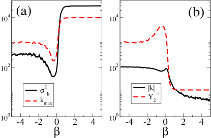
Figure 1: (color online) Properties of the layer degree distribution for $\alpha=1.0$ as a function of $\beta$. (a) Variance $\sigma^{2}_{k}$ of the degree sequence (solid black) and maximum degree $k_{\rm max}$ (dashed red). (b) Number of different degree classes $|k|$ (solid black) and participation ratio $Y_{2}^{-1}$ (dashed red). There is a clear dependence of the network structure on the attachment exponent $\beta$. The plots correspond to a multiplex network with $N=10.000$, $m=3$, $m_{0}=3$.

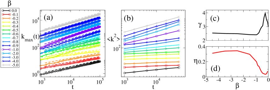
Figure 2: (color online) The scalings with $t$ of the degree $k_{\rm max}(t)$ of the largest hub (a) and of the fluctuations of the degree sequence $\langle{k^{2}}\rangle$ (b) for $\alpha=1.0$ and for different values of $\beta\leq 0$ suggest that the degree distribution of each layer is a power-law $P(k)\sim k^{-\gamma}$ (the plots are vertically displaced to enhance readability). (c) The exponent $\gamma$ of the degree distribution is equal to $3.0$ when $\beta=0$, as in the case of classical linear preferential attachment, has a maximum around $\beta\simeq-0.3$ and converges to $\gamma\simeq 2.5$ when $\beta\rightarrow-\infty$. (d) Similarly, the exponent $\eta$ has a minimum for $\beta~{}\simeq 0.3$ and converges towards $\eta\simeq-0.3$ for negative values of $\beta$.

When $\beta\neq 0$ the growth process can produce multiplex networks with homogeneous, heterogeneous or condensed degree distribution on each layer, characterized by either assortative or disassortative inter-layer degree correlation patterns, depending on the sign of $\beta$. In Fig. 1 we report the results obtained by simulating the growth of a multiplex for $\alpha=1.0$ and $\beta$ in the range $[-5,5]$. In order to characterize the degree distributions of the two layers we plot, as a function of $\beta$, the variance $\sigma^{2}_{k}$ of the degree distribution, the maximum degree $k_{\rm max}$, the number $|k|$ of different degree classes present in each layer, and the participation ratio $Y_{2}^{-1}$. Given a degree sequence $\{k_{1},k_{2},\ldots,k_{N}\}$, $Y_{2}^{-1}$ is defined as Derrida:1987

$$Y_{2}^{-1}=\left[\sum_{i}\left(\frac{k_{i}}{\sum_{j}k_{j}}\right)^{2}\right]^{-1}.$$ (4)

It is easy to show that $Y_{2}^{-1}\sim O(N)$ when $k_{i}=\langle{k}\rangle\>$ for all $i$, i.e. for homogeneous degree distributions, while $Y_{2}^{-1}=c\ll N$ if most values of $k_{i}$ are equal, except for a few nodes for which we have $k_{i*}\simeq N$, i.e. in the presence of a condensate state where a few nodes connect to nearly all the other nodes of a layer. When $\alpha=1$ and $\beta$ is positive, we observe a transition to a condensed state, characterized by small $|k|$, large $\sigma^{2}_{k}$, $k_{\rm max}\sim O(N)$, and $Y_{2}^{-1}\sim O(1)$, signalling the existence of a few dominant nodes. Conversely, for negative values of $\beta$ we obtain heterogeneous degree distributions (large values of $|k|$, relatively large values of $k_{\rm max}$, $\sigma^{2}_{k}$ and $Y_{2}^{-1}$). In particular, these distribution are power-laws. In fact, as shown in. Fig. 2(a)-(b), for $\beta\leq 0$ the degree $k_{\rm max}(t)$ of the largest hub of the graph at time $t$ scales as $t^{\varepsilon},\quad\varepsilon>0$ and the fluctuations of the degree distributions $\langle{k^{2}}\rangle$ scale as $t^{\eta},\quad\eta>0$.

In Fig. 2(c) we report the exponent $\gamma$ of the power law distribution of the two layers, whose value clearly depends on $\beta$. In particular, for $\beta=0$ we recover $\gamma=3.0$, as in the standard single-layer linear preferential attachment. When $\beta\rightarrow-\infty$ then $\gamma$ converges to $\gamma\simeq 2.5$. When $\beta$ is negative and close to zero, we observe a strange phenomenon, which is also responsible for the peaks in $|k|$, $Y_{2}^{-1}$, $\sigma^{2}_{k}$ and $k_{\rm max}$ shown in Fig. 1. In this region, as we increase $\beta$ the distribution becomes first more homogeneous (with a peak of $\gamma\simeq 4$ for $\beta\simeq-0.3$) and then again more heterogeneous, up until $\gamma=3.0$ for $\beta=0$.

This apparently strange behavior can be explained by considering that for $\beta<0$ the two layers are competing, i.e. a node having high degree on one layer will tend to have small degree on the other layer. In this case, a small negative value of $\beta$ actually reduces the heterogeneity of the attachment probability distribution that we have for $\beta=0$, allowing small-degree nodes (for which the effect of layer competition is mitigated by the fact that $\beta$ is negative and close to zero) to acquire more edges. Conversely, when the value of $\beta$ becomes smaller then local fluctuations start to play a fundamental role, and the distribution becomes more heterogeneous again.

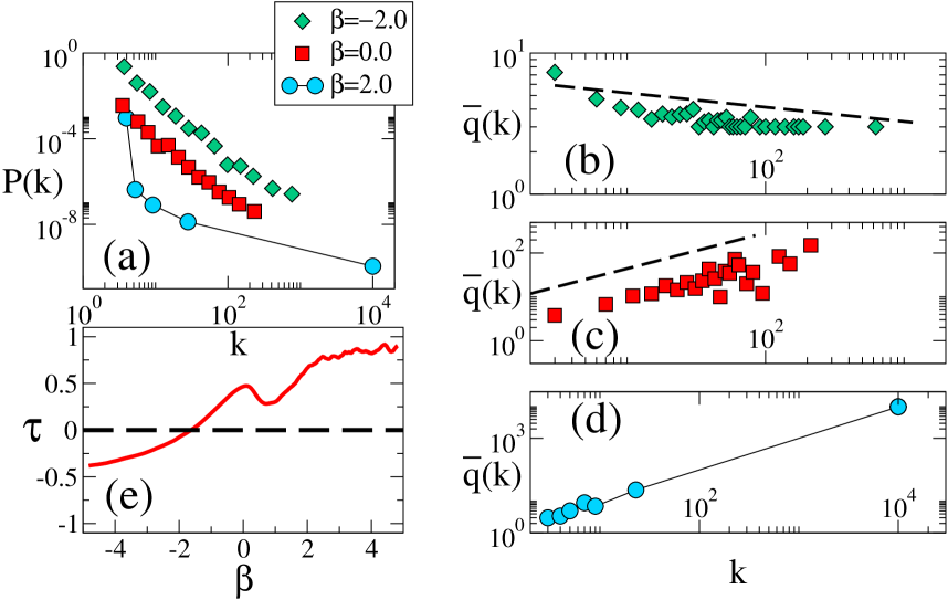
Figure 3: (color online) (a) Typical degree distributions for $\beta=-2.0$ (green diamonds), $\beta=0.0$ (red squares) and $\beta=2.0$ (cyan circles) when $\alpha=1.0$. According to the value of $\beta$, the degree distribution of a layer can be either a power-law ($\beta\leq 0$) or condensed, i.e. characterized by the presence of a super-hub which attracts an extensive fraction of edges. The corresponding pattern of inter-layer degree correlations $\overline{q}(k)$ in the three cases [panels (b)-(d)] and the plot of the inter-layer degree correlation coefficient $\tau$ [Panel (e)] confirm that both positive and negative correlations can be obtained by tuning $\beta$.

Three typical examples of degree distributions obtained for different values of $\beta$ are reported in Fig.3(a), in particular for $\beta=-2.0,0.0,2.0$. When $\beta=2.0$ we observe a homogeneous distribution for small values of $k$, and one node acquires a finite fraction of the edges, i.e. the network is condensed. For $\beta=0.0$ the degree distribution is a power-law with exponent $\gamma\simeq 3.0$ Nicosia2013 . Finally, for $\beta=-2.0$ the degree distribution can be fitted by a power-law with exponent $\gamma\simeq 2.5$.

Interestingly, the value of $\beta$ also determines the sign and value of inter-layer degree correlations, as confirmed by the plot of the average degree $\overline{q}(k)$, at layer $2$, of nodes having degree $k$ at layer $1$, shown in Fig. 3(b)-(d) Nicosia2013 . It is clear that, by tuning $\beta$, one can obtain either positive ($\beta=2.0$, and $\beta=0.0$) or negative ($\beta=-2$) inter-layer degree correlations. Finally, in Fig. 3(e) we plot as a function of $\beta$ the value of the Kendall’s rank correlation coefficient $\tau$ computed on the degree sequences of the two layers (see Appendix). For $\beta<0$ we have disassortative inter-layer degree correlations ($\tau<0$), meaning that a hub on one layer is a poorly-connected node on the other layer, while for $\beta>0$ the degrees of the two replicas of the same node are positively correlated ($\tau>0$).

III Mean-field approximation

The mean-field approach has been proven to be extremely good in making qualitative predictions on the degree distribution of growing network models. Here we report convincing evidence that this approach is not able to capture essential properties of the proposed non-linear growth model. In fact in this model stochastic effects are fundamental to describe the evolution of the system. As we will see in a moment, the conclusion of the mean-field theory is that the expected degrees of the same node in the two layers are equal, irrespective of the values of the two exponents $\alpha$ and $\beta$. However, such a conclusion is in clear disagreement with the results obtained by numerical simulation and reported, for instance, in Fig. 3, which indeed confirm that for some combinations of the exponents $\alpha$ and $\beta$ the degrees of a node at the two layers can be negatively correlated.

In the mean-field approximation the degree of a node $i$ at time $t$ acquires a deterministic value equal to its average degree in the stochastic model. If we indicate by $\kappa_{i}(t)$ and by $\phi_{i}(t)$ the average degree of node $i$ on layer 1 and on layer 2 respectively, the mean-field approximation assumes that the degree $k_{i}(t)$ of a node $i$ in layer 1 is equal to $\kappa_{i}(t)$, i.e. $k_{i}(t)=\kappa_{i}(t)$ and similarly that the degree in layer 2 $q_{i}(t)$ of node $i$ at time $t$ is given by $q_{i}(t)=\phi_{i}(t)$. Since, in this approximation, the average number of links that at time $t$ a node $i$ acquires in layer 1 is given by

$$m\frac{f(\kappa_{i},\phi_{i})}{\sum_{j}f(\kappa_{j},\phi_{j})},$$ (5)

while the average number of links that a node $i$ acquires at time $t$ in layer 2 is given by

$$m\frac{f(\phi_{i},\kappa_{i})}{\sum_{j}f(\phi_{j},\kappa_{j})},$$ (6)

when $f(\kappa,\phi)=\kappa^{\alpha}\phi^{\beta}$ and $f(\phi,\kappa)=\phi^{\alpha}\kappa^{\beta}$ as in Eq.(3), the mean-field equations for $\kappa_{i}(t)$ and $\phi_{i}(t)$ at large times $t\gg 1$ read

$$\frac{d\kappa_{i}}{dt}=\frac{\kappa_{i}^{\alpha}\phi_{i}^{\beta}}{Ct},~{}~{}~{}~{}~{}~{}~{}~{}~{}~{}~{}~{}~{}\frac{d\phi_{i}}{dt}=\frac{\phi_{i}^{\alpha}\kappa_{i}^{\beta}}{Ct},$$ (7)

with the constant $C$ to be self-consistently determined as

$$C=\lim_{t\to\infty}\frac{\sum_{i=1}^{t}{\kappa_{i}^{\alpha}\phi_{i}^{\beta}}}{mt}.$$ (8)

Assuming that $C$ is a constant, the Eqs. $(\ref{mf})$ can be rewritten as

$$\kappa_{i}^{\beta-\alpha}\frac{d\kappa_{i}}{d\ln t}=\frac{1}{C}{(\kappa_{i}\phi_{i})^{\beta}}=\phi_{i}^{\beta-\alpha}\frac{d\phi_{i}}{d\ln t}.$$ (9)

Therefore we find for $\beta-\alpha\neq-1$

$$\frac{d\left[\kappa_{i}^{\beta-\alpha+1}-\phi_{i}^{\beta-\alpha+1}\right]}{d\ln t}=0,$$ (10)

while we have for $\beta-\alpha=-1$

$$\frac{d\ln\kappa_{i}-\ln\phi_{i}}{d\ln t}=0.$$ (11)

Therefore, if we consider the initial conditions $\kappa_{i}(t_{i})=\phi_{i}(t_{i})=m$ the mean-field approach implies always $\kappa_{i}(t)=\phi_{i}(t)$. Inserting this solutions in the Eqs. $(\ref{mf})$ we get

$$\frac{d\kappa_{i}}{dt}=\frac{\kappa_{i}^{\alpha+\beta}}{Ct}$$ (12)

yielding the solution

$$\kappa_{i}(t)=m\left(\frac{t}{t_{i}}\right)^{1/C}$$ (13)

for $\alpha+\beta=1$, and the solution

$$\kappa_{i}(t)=\left[m^{1-(\alpha+\beta)}+\frac{1-\alpha-\beta}{C}\ln\left(\frac{t}{t_{i}}\right)\right]^{1/(1-(\alpha+\beta))}$$ (14)

for $\alpha+\beta<1$.

For $\alpha+\beta>1$ we observe a singularity in the solution for $\kappa_{i}(t)$ indicating the fact that the self-consistent equation for $C$ cannot be satisfied. By studying the master equation we will show that for $\alpha+\beta>1$ we observe a condensation phase transition. Starting form the solution given by Eq. (13) and Eq.(14) the predicted degree distribution is scale free with power-law exponent $\gamma=1+1/C$ for $\alpha+\beta=1$ and a Weibull distribution for $\alpha+\beta<1$.

Overall we can say that the mean-field approach provides a solution that reflects the symmetry of the model in the two layers. Nevertheless this approach mostly fails in characterizing the correlations between the degrees of the same node in different layers. As we said before, the behavior of the model and its predictions $\kappa_{i}(t)=\phi_{i}(t)$ are not supported by the simulations because the dynamics of the model is strongly affected by stochasticity and noise. In particular we argue that the strong deviations from the mean-field behavior that we observe in the simulations are due to the fundamental role played by stochastic effects on the degrees of the nodes recently arrived in the network. In fact these nodes will have a small degree in both layers and the fluctuations on these quantities will strongly affect the linking probability distribution.

IV Master equation

More theoretical insights about the model defined by Eq. (2) and Eq. (3) come from the solution of the master equation of the system, which accounts for the expected number of nodes $N_{k,q}$ with $k$ links in layer 1 and $q$ links in layer 2. Let us consider for simplicity the case $m=1$. The master equation needs to take into account that at any time $t$ one of the following events can occur:

1. The number of nodes $N_{k,q}$ with degree $k$ in layer 1 and degree $q$ in layer 2 increases by one if the new node links in layer 1 but not in layer 2 to a node of degree $k-1$ in layer 1 and degree $q$ in layer 2.

2. The number of nodes $N_{k,q}$ with degree $k$ in layer 1 and degree $q$ in layer 2 increases by one if the new node links in layer 2 but not in layer 1 to a node of degree $k$ in layer 1 and degree $q-1$ in layer 2.

3. The number of nodes $N_{k,q}$ with degree $k$ in layer 1 and degree $q$ in layer 2 increases by one if the new node links in layer 1 and also in layer 2 to a node of degree $k-1$ in layer 1 and degree $q-1$ in layer 2.

4. The number of nodes $N_{k,q}$ with degree $k$ in layer 1 and degree $q$ in layer 2 decreases by one if the new node links in layer 1 to a node of degree $k$ in layer 1 and degree $q$ in layer 2.

5. The number of nodes $N_{k,q}$ with degree $k$ in layer 1 and degree $q$ in layer 2 decreases by one if the new node links in layer 2 to a node of degree $k$ in layer 1 and degree $q$ in layer 2.

Moreover, for $k=m$ and $q=m$ the average number of nodes $N_{k,q}$ with degree $k$ in layer 1 and degree $q$ in layer 2 increases by one at each time step, since the newly arrived node has degrees $k=m$ and $q=m$. Taking into account all these possibilities, we can write the master equation as

$$N_{k,q}(t+1) = N_{k,q}(t)+\delta_{k,m}\delta_{q,m}+\frac{f(k-1,q)}{{\cal M}(t)}\left(1-\frac{f(q,k-1)}{{\cal M}(t)}\right)N_{k-1,q}(t)(1-\delta_{k,m})$$ (15)

$$+\frac{f(q-1,k)}{{\cal M}(t)}\left(1-\frac{f(k,q-1)}{{\cal M}(t)}\right)N_{k,q-1}(t)(1-\delta_{q,m})-\left[\frac{f(q,k)+f(k,q)}{{\cal M}(t)}-\frac{f(k,q)f(q,k)}{[{\cal M}(t)]^{2}}\right]{N_{k,q}(t)}$$

$$+\frac{f(q-1,k-1)f(k-1,q-1)}{[{\cal M}(t)]^{2}}N_{k-1,q-1}(t)(1-\delta_{q,m})(1-\delta_{k,m})$$

where $k,q\geq m$, $f(k,q)=k^{\alpha}q^{\beta}$, $\delta_{\bullet,\bullet}$ is the Kronecker delta and ${\cal M}(t)$ is given by:

$${\cal M}(t)=\sum_{k,q}f(k,q)N_{k,q}(t)=\sum_{k,q}f(q,k)N_{k,q}(t)$$ (16)

Eq. (15) can be solved by using techniques similar to those adopted for single-layer networks or for multiplex networks with linear or semi-linear attachment kernels krapivsky ; Dorogovtsev ; Nicosia2013 . In particular, by solving the master equation we obtain an analytical explanation for the appearance of a condensed phase. In fact, the master equation depends on the quantity ${\cal M}(t)$ which satisfies, in the thermodynamic limit $t\to\infty$, the relation

$${\cal M}(t)=\sum_{k,q}f(k,q)N_{k,q}(t)=\sum_{k,q}f(q,k)N_{k,q}(t).$$ (17)

Assuming that the normalization sum scales like ${\cal M}(t)\propto t$, i.e. $\lim_{t\rightarrow\infty}{{\cal M}(t)/t}=C$ with $C$ constant, we can derive a recursive expression for $P_{k,q}=\lim_{t\to\infty}N_{k,q}(t)/t$. However, the hypothesis ${\cal M}(t)\propto t$ depends on the value of the exponents $(\alpha,\beta)$ and in general is not satisfied. A deviation from this scaling indicates that in each layer we have a node that is grabbing an extensive number of links $k_{\rm max}\simeq t,q_{\rm max}\simeq t$, i.e. we are in a condensed network phase.

IV.1 Conditions for condensation

In order to show in which region of the phase space condensation occurs we first find a sufficient condition for condensation and then we will show that this condition is also a necessary one. We make use of the master equation to estimate ${\cal M}(t)$, respectively for $\beta\leq 0$ and $\beta>0$, by considering (without loss of generality) the case $m=1$. We observe that for $\beta\leq 0$ at each time $t$ there are no vertices that in layer 1 have degree greater than $k=t$, therefore the master equation given by Eq. (15) becomes

$$N_{k,1}(k)=\frac{(k-1)^{\alpha}}{{\cal M}(k-1)}\left(1-\frac{(k-1)^{\beta}}{{\cal M}(k)}\right)N_{k-1,1}(k-1)$$ (18)

But for large times $\frac{(k-1)^{\beta}}{{\cal M}(k)}\ll 1$. Moreover the fractions $N_{k-1,1}(k-1)/N_{k,1}(k)\geq 1$ since only the first node of the network can have degree $k$ equal to the time $t=k$. Consequently

$${\cal M}(t)\geq{t^{\alpha}}.$$ (19)

Instead, if $\beta>0$ then at time $t$ there are no nodes that have at the same time degree in layer 1 greater than $k=t$ and degree in layer 2 greater then $k=t$. In this case the master equation given by Eq. (15) becomes

$$N_{k,k}(k)=\frac{(k-1)^{2(\alpha+\beta)}}{[{\cal M}(k-1)]^{2}}N_{k-1,k-1}(k-1).$$ (20)

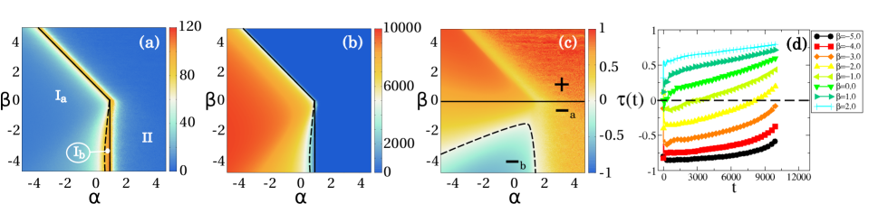
Figure 4: (color online) As a function of the two parameters $\alpha$ and $\beta$ we report, by means of a color code: (a) the number of distinct degree classes $|k|$, (b) the participation ratio $Y_{2}^{-1}$, and (c) the Kendall’s $\tau$ correlation coefficient. The solid black lines in panel (a) and (b) separate the non-condensed (region I) from the condensed phase (region II, small $|k|$, small $Y_{2}^{-1}$). In region I we can have either homogeneous (region ${\rm I_{a}}$) or heterogeneous degree distributions (region ${\rm I_{b}}$). The solid black line in panel (c) separates the two regions with positive (region $\bm{+}$) and negative inter-layer degree correlations (region $\bm{-}$), respectively corresponding to $\beta>0$ and $\beta<0$. The value of $\tau$ for the whole multiplex is negative only in region $\bm{-_{b}}$. In panel (d) we show the plot of $\tau(t)$, which is the Kendall’s $\tau$ restricted to the nodes arrived up to time $t$. The dashed black line corresponds to $\tau=0$ and is reported for visual reference.

Notice that the fractions $N_{k-1,k-1}(k-1)/N_{k,k}(k)\geq 1$ since only the first node of the network can have degrees $(k,q)$ equal to $(t,t)$, where $t$ is the time. Therefore we get that

$${\cal M}(t)\geq\left\{\begin{array}[]{ccc}t^{\alpha}&\mbox{if}&\beta\leq 0\\ t^{\alpha+\beta}&\mbox{if}&\beta>0\end{array}\right.$$

This means that for $\alpha>1$ and $\beta<0$ or for $\beta>0$ and $\alpha>1-\beta$

$${\cal M}(t)\geq t^{\xi},\quad\forall\xi>1.$$ (21)

This is a sufficient condition to have condensation, since in this case the expected number of nodes that at time $t$ have degrees $k=1,q=1$ scales with $t$, i.e. $N_{1,1}(t)\simeq t$. In fact, starting from the master equation, $N_{1,1}(t)$ satisfies the following relation

$$\frac{dN_{1,1}(t)}{dt}=-2\frac{1}{{\cal M}(t)}N_{1,1}(t)+1,$$ (22)

where in writing this equation we have neglected higher order terms in $[{\cal M}(t)]^{-1}$. If Eq. (21) is satisfied, then the first term in the right-hand side of Eq. (22) is negligible and we have $N_{1,1}(t)\simeq t$ for large $t$. This implies that the number of nodes with degrees different from $(k=1,q=1)$ is negligible, so that in this region we have a condensation phenomenon with few nodes grabbing an extensive number of connections.

Let us now show that the condition $\beta<0$, $\alpha>1$ and $\beta>0$, $\alpha+\beta>1$ is also necessary for condensation. Let us assume that we have a condensation of the links. In this scenario, we will have for $\beta<0$ one node with degree $k=t$ on layer 1, say node $i$, and another node with degree $q=t$ on layer 2, say node $j$; conversely, for $\beta>0$ we will expect to have exactly one node, say node $i$, having degrees $(k,q)=(t,t)$. Since we have condensation then we can write an upper bound to ${\cal M}(t)=\sum_{k,q}k^{\alpha}q^{\beta}N_{k,q}$, by taking into account only the contribution of the condensed nodes:

$${\cal M}(t)\leq\left\{\begin{array}[]{ccc}t^{\alpha}&\mbox{for}&\beta\leq 0\\ t^{\alpha+\beta}&\mbox{for}&\beta>0\end{array}\right.$$ (23)

Putting Eq. (23) together with the lower bound given by Eq. (21) we find that ${\cal M}(t)$ satisfies the scaling

$${\cal M}(t)\simeq\left\{\begin{array}[]{ccc}t^{\alpha}&\mbox{for}&\beta\leq 0\\ t^{\alpha+\beta}&\mbox{for}&\beta<0\end{array}\right.$$

But we know that ${\cal M}(t)\propto t^{\xi}$ with $\xi\geq 1$, therefore we confirm that if the condensation transition occurs then either $\alpha>1$ and $\beta\leq 0$ or $\alpha+\beta>1$ and $\beta>0$. Therefore the condensation transition occurs only in the region $\beta<0$ $\alpha>1$ or in the region $\beta>0$, $\alpha>1-\beta$. In particular, for $\beta>0$ the same node will be the condensate node in both layers, while for $\beta<0$ the condensate node in one layer will not be the condensate node in the other layer. When $\beta=0$ the condensate nodes in the two layers might be either the same node or different nodes in different realizations.

IV.2 Solution of the master equation in the non condensed phase

We consider now the master equation in the non condensed phase where ${\cal M}(t)\simeq Ct$ with $C>0$ independent on $t$, for $t\gg 1$. As we have seen above, this implies that the parameters $\alpha,\beta$ satisfy the conditions: $\alpha\leq 1$ and $\beta<0$ or $\beta>0$ and $\alpha\leq 1-\beta$. In this region of the phase space, we have always $f(k,q)/{\cal M}(t)\ll 1$ and therefore we can neglect the terms proportional to $[{\cal M}(t)]^{-2}$ in the rate equation, finding the master equation for evolving multiplex in the non condensed phase, i.e.

$$\frac{dN_{k,q}(t)}{dt} =\frac{\displaystyle A_{k-1,q}}{\displaystyle t}N_{k-1,q}(t)+\frac{\displaystyle B_{k,q-1}}{\displaystyle t}N_{k,q-1}(t)+$$ (24)

$$-\left[\frac{\displaystyle A_{k,q}+B_{k,q}}{\displaystyle t}\right]N_{k,q}(t)+\delta_{k,m}\delta_{q,m}$$

where we have put

$$A_{k,q}=\frac{k^{\alpha}q^{\beta}}{C},~{}~{}~{}~{}~{}~{}~{}~{}~{}~{}~{}~{}~{}~{}~{}B_{k,q}=\frac{q^{\alpha}k^{\beta}}{C},$$ (25)

and $C$ is a constant that can be determined self-consistently as

$$C=\lim_{t\to\infty}\frac{1}{t}{\sum_{k,q}k^{\alpha}q^{\beta}N_{k,q}}(t).$$ (26)

Assuming $N_{k,q}\simeq tP_{k,q}$ valid in the large time limit, we can solve for $P_{k,q}$ and we get

$$\begin{array}[]{cll}P_{m,q}&=&\left(\prod_{j=m}^{q}\frac{B_{k,j-1}}{1+A_{k,j}+B_{k,j}}\right)P_{m,m}\\ P_{k,q}&=&\sum_{r=1}^{q}\left(\prod_{j=r+1}^{q}\frac{B_{k,j-1}}{1+A_{k,j}+B_{k,j}}\right)\frac{A_{k-1,r}}{1+A_{k,r}+B_{k,r}}P_{k-1,r}\end{array}$$

These recursive equations can be used to solve numerically for the joint degree distribution of the degrees in the two layers, but unfortunately for $\beta\neq 0$ there is no closed form analytical solution to these equations.

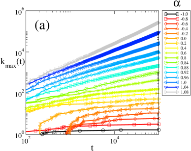
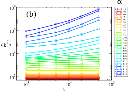
Figure 5: (a) The scaling of the degree $k_{\rm max}(t)$ of the largest hub of a layer depends on the value of $\alpha$ (here we fixed $\beta=-1.0$). In particular, $k_{\rm max}(t)\sim t^{\varepsilon}$ only for $\alpha$ larger than $0.6\sim 0.8$, suggesting that the degree distribution becomes heterogeneous when $\alpha$ is closer to the critical value for condensation ($\alpha=1.0$). (b) The value of $\langle{k^{2}}\rangle$ as a function of $t$, for $\beta=-1.0$ and different values of $\alpha$. If we start from $\alpha=-1.0$ and keep increasing it, we initially notice no scaling at all with $t$, up until $\alpha\simeq 0.8$, when $\langle{k^{2}}\rangle\sim t^{\eta}$. This means that for $0.8<\alpha<1.0$ the second moment of the degree distribution diverges with $t$.

V Numerical Results

The predictions obtained by solving the master equation of the model are in very good agreement with the phase diagram of the system obtained through simulations, reported in Fig. 4(a)-(b) ($N=10.000$, $m=3$, $m_{0}=3$). In these figures we show, for each value of the two parameters $\alpha$ and $\beta$, the corresponding values of $|k|$ (a) and $Y_{2}^{-1}$ (b), which allow us to visualize the two separate regions of the phase space. In region I the degree distribution is not condensed, while in region II we observe condensation as indicated by both a small value of $|k|$ and of $Y_{2}^{-1}$. The shape of the boundary between the two regions agrees very well with the analytical prediction provided by the solution of the master equation in the thermodynamic limit (indicated by the solid lines in panel (a) and panel (b)). We notice that region I can be further divided into two separate sub-regions, according to the fact that the resulting degree distribution at each layer is homogeneous (region ${\rm I_{a}}$) or heterogeneous (region ${\rm I_{b}}$).

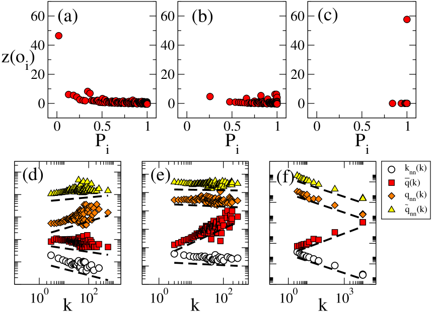
Figure 6: (color online) In the top panels we report the multiplex cartography of networks obtained by setting, respectively, (a) $\beta=-1.0$, (b) $\beta=0.0$ and (c) $\beta=1.0$ when $\alpha=1.0$. For $\beta<0$ there is a high heterogeneity of node roles, and hubs tend to be focused. Conversely, for $\beta>0$ all nodes tend to be genuinely multiplex, i.e. to have similar degrees on both layers. In the bottom panels we plot the intra-layer, inter-layer and mixed correlations respectively for (d) $\beta=-1.0$, (e) $\beta=0.0$ and (f) $\beta=1.0$ when $\alpha=1.0$.

It is interesting to analyze the transition to condensation as a function of $\alpha$ at fixed $\beta<0$, i.e. region $I_{b}$. In particular, we are interested in checking whether the degree distribution becomes a power–law before we reach the condensation transition (we already know that at the boundary of the condensation transition the degree distribution is a power-law, with an exponent which depends on $\beta$, as discussed in Sec. II). Therefore, we analyzed the scaling of the degree of the largest hub $k_{\rm max}(t)$ and of the fluctuations of the degree distribution $\langle{k^{2}}\rangle$ as a for increasing values of $\alpha$. The results corresponding to $\beta=-1.0$ are reported in Fig.5(a) and Fig. 5(b). Notice that for $\alpha<0$ we observe homogeneous degree distributions, i.e. no scaling of fluctuations with $N$ and a logarithmic scaling of $k_{\rm max}(t)$, while for $\alpha=1.0$ we have $k_{\rm max}(t)\sim t^{1/2}$, which corresponds to $\gamma=3.0$. However, we observe that $\langle{k^{2}}\rangle$ scales as $t^{\eta}$ already for $\alpha<1.0$, and in particular in the region $0.8<\alpha<1.0$. Also, in this region $k_{\rm max}(t)$ scales as $t^{\varepsilon}$, indicating that in region $I_{b}$ the degree distribution of each layer is a power-law.

Concerning the sign of inter-layer correlations, in Fig. 4(c) we report the Kendall’s correlation coefficient $\tau$ of the degree sequences at the two layers, where the two regions where inter-layer degree correlations are respectively positive (region $\bm{+}$) and negative (region $\bm{-}$) are separated by a solid black line. It is interesting to note that a multiplex can exhibit either positive or negative inter-layer correlations independently of the fact that its layers have homogeneous or heterogeneous distributions. While from the linking probabilities given by Eq. (2)-(3) we expect $\tau>0$ when $\beta>0$, when $\beta<0$ the degrees of a node in the two layers tend to be negatively correlated. However, the interpretation of the phase diagram of $\tau$ for negative $\beta$ is less trivial, and the shape of the boundary between the regions $\bm{-_{a}}$ and $\bm{-_{b}}$ needs some explanation. In fact, when $\beta<0$ Eq. (3) implies that if a node has high degree in one layer, it will have low probability to acquire new links in the other layer, so that the degrees of the old nodes of the network will be negatively correlated. This is clear by looking at Fig. 4(d), which confirms that for $\beta<0$ the inter-layer degree correlations of older nodes are always negative.

However, for some values of $\beta$ the value of $\tau$ computed on the whole network could be positive, due to the presence of a large majority of younger nodes having small degrees on both layers (i.e. fickle nodes), whose values are mostly determined by stochastic fluctuations. In general, for large negative values of $\beta$ the fraction of fickle nodes is reduced, until it becomes zero for $\beta<\beta_{c}(\alpha)$ (the dashed line in Fig. 4(c) corresponds to the values of $\beta_{c}(\alpha)$), and in this case all the nodes have negative correlated degrees, resulting in a negative value of $\tau$. We notice that the existence of two sub-regions in the phase diagram of $\tau$ for $\beta<0$ is not a finite-size effect, as confirmed by the results shown in Appendix Fig. A-1.

VI Multiplex cartography

The authors of Ref. battiston have recently introduced the concept of multiplex cartography, which is in the same spirit of the network cartography proposed by Guimerá and Amaral in Ref. Guimera05 ; GuimeraNature05 . Multiplex cartography is based on two measures, namely the Z-score of the overlapping degree of a node:

$$z(o_{i})=\frac{o_{i}-\langle o\rangle}{\sigma_{o}}$$ (27)

where $o_{i}=\sum_{\alpha}k^{[\alpha]}_{i}$ while $\langle{o}\rangle$ and $\sigma_{o}$ are the average and standard deviation of $o_{i}$ over all the nodes, and the multiplex participation coefficient:

$$P_{i}=\frac{M}{M-1}\left[1-\sum_{\alpha=1}^{M}\left(\frac{k_{i}^{[\alpha]}}{o_{i}}\right)^{2}\right].$$ (28)

The multiplex participation coefficient of a node characterizes its involvement in the layers of the multiplex. In fact, $P_{i}$ tends to $1$ if node $i$ has exactly the same degree on all the $M$ layers, while $P_{i}=0$ if node $i$ is isolated on all the $M$ layers but one. With respect to the Z-score of their overlapping degree, we distinguish hubs, for which $z(o_{i})\geq 2$, from regular nodes, for which $z(o_{i})<2$. With respect to the multiplex participation coefficient, we call focused those nodes for which $0\leq P_{i}\leq 0.3$, mixed the nodes having $0.3<P_{i}\leq 0.6$ and truly multiplex (or even simply multiplex) the nodes for which $P_{i}>0.6$. The scatter-plot of $z(o_{i})$ and $P_{i}$ provides information about the patterns of participation across nodes of different degree classes, and gives insight about the different roles played by nodes.

In Fig. 6(a)-(c) we report the multiplex cartography diagrams for different values of $\beta$ ($\alpha=1.0$). It is interesting to notice that layer competition (i.e., $\beta<0$) enhances the variability of the multiplex cartography but produces multiplexes in which hubs are predominantly focused (top-left corner of the plots) while poorly-connected nodes are predominantly multiplex. Conversely, strong layer concordance (i.e., $\beta>0$) tends to produce multiplexes in which nodes belong to just a few different classes, i.e. either multiplex hubs or multiplex nodes.

VII Mixed correlations

Since the combination of $\alpha$ and $\beta$ allows to produce multiplex graphs having either assortative or disassortative intra-layer degree-degree correlations and positive, null or negative inter-layer degree correlations, it is interesting to look at the combination of intra-layer and inter-layer correlations. In particular, we might ask whether a node being a hub on layer $1$ is preferentially connected on layer $2$ with other hubs or instead with leaves. So in general we can be interested in assessing whether:

1. a hub tends to be connected with other hubs or to poorly-connected nodes (intra-layer correlations);

2. a hub on one layer tends to be either a hub or a poorly-connected node in the other layer (inter-layer correlations);

3. a hub in one layer has neighbors in the other layer who are connected either to other hubs or poorly-connected nodes(type-1 mixed correlations).

4. the neighbors of a hub in one layer are either hubs or poorly-connected nodes in the other layer (type-2 mixed correlations).

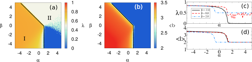
Figure 7: (color online) Phase diagrams of (a) the average shortest path length $\langle{l}\rangle$ and (b) the multiplex interdependence $\lambda$ for $N=2000$, $m=3$, $m_{0}=3$, and three corresponding cross-cut sections for fixed values of $\beta$ [panel (c) and panel (d)]. As in Fig. 4, the black solid lines separate the non condensed (region $\rm I$) from the condensed phase (region $\rm II$). In the non-condensed phase both $\langle{l}\rangle$ and $\lambda$ exhibit small variations, while the interdependence in the condensed phase is $\lambda=0.5$ for $\beta>0$ and $\lambda=0.0$ for $\beta<0$, in agreement with the fact that for $\beta>0$ the same node is condensed in both layers, while for $\beta<0$ the condensed nodes in the two layers are distinct.

We measure type-1 mixed correlations using the quantity:

$$k_{nn}(q)=\sum_{k}P(k=k_{i}|q=q_{i})\frac{1}{k_{i}}\sum_{j}a^{[1]}_{ij}k_{j}$$ (29)

which is the average degree of first neighbors on layer $1$ of a node having degree $q$ at layer $2$. Similarly, we can define the dual quantity:

$$q_{nn}(k)=\sum_{q}P(q=q_{i}|k=k_{i})\frac{1}{q_{i}}\sum_{j}a^{[2]}_{ij}q_{j}$$ (30)

If the plot of $k_{nn}(q)$ is an increasing (decreasing) function of $q$, then we say that the mixed correlations of layer $1$ with respect to layer $2$ are positive (negative), or assortative (disassortative).

Type-2 mixed correlations can be quantified through the following expression:

$$\widetilde{q}_{nn}(k)=\frac{1}{N_{k}}\sum_{i}\delta(k_{i},k)\frac{1}{k_{i}}\sum_{j}a_{ij}^{[1]}q_{j}$$ (31)

which corresponds to the average degree at layer $2$ of the neighbors on layer $1$ of a node having degree $k$ on layer $1$, and by the dual expression:

$$\widetilde{k}_{nn}(q)=\frac{1}{N_{q}}\sum_{i}\delta(q_{i},q)\frac{1}{q_{i}}\sum_{j}a_{ij}^{[2]}k_{j}$$ (32)

Here $N_{k}$ (resp. $N_{q}$) indicates the number of nodes having degree equal to $k$ (resp. $q$) on layer $1$ (resp. on layer $2$). In Fig. 6(d)-(f) we show the intra- inter- and mixed correlation patterns obtained for several values of $\beta$. Interestingly, for different values of the parameters one obtains different intra- and inter-layer correlation patterns, but also assortative or disassortative mixed correlations.

VIII Distance and interdependence

Despite the main focus of the present work is on the properties of degree distribution and inter-layer degree correlations, we have also explored the distribution of shortest path length and the actual organization of shortest paths in the multiplex as a function of the two parameters $\alpha$ and $\beta$. It is important to notice that in a multiplex network the shortests paths between any pair of nodes are not limited to just one layer but can instead span both layers. Therefore, aside with the classical measure of characteristic path length:

$$\langle{l}\rangle=\frac{1}{N(N-1)}\sum_{i}\sum_{j<i}d_{ij},$$ (33)

which is just the average over all possible pairs of nodes of the distance $d_{ij}$ between node $i$ and node $j$, we also computed the multiplex interdependenceMorris:2012 ; Nicosia2013 :

$$\lambda=\frac{1}{N}\sum_{i}\sum_{j\neq i}\frac{\psi_{ij}}{\sigma_{ij}}.$$ (34)

The quantity $\lambda\in[0,1]$ is the average ratio between the number $\psi_{ij}$ of shortest paths between node $i$ and node $j$ which use edges lying on both layers and the total number $\sigma_{ij}$ of shortest paths between $i$ and $j$ in the multiplex. When $\lambda\simeq 0$ then almost all shortest paths run in just one layer, while at the other extreme $\lambda\simeq 1$ all shortest paths use edges in both layers.

In Fig. 7(a)-(b) we report the value of $\lambda$ and $\langle{l}\rangle$ for a synthetic multiplex of $N=2000$ nodes as a function of $\alpha$ and $\beta$. Notice that the behaviour of $\langle{l}\rangle$ closely mirrors that of the participation ratio reported in Fig. 4. As expected, the characteristic path length is smaller in the condensed phase, due to the presence of condensed nodes which are connected to virtually all the other nodes, and is larger in the non-condensed phase. The behavior of $\lambda$ is more interesting. In fact, the non-condesed phase is characterised by a relatively high interdependence, and its value (which is almost always confined in the interval $[0.7:0.9]$) does not heavily depend on the actual value of $\alpha$ and $\beta$. In the condensed phase, instead, we spot two different sub-regions. For $\beta>0$ we have $\lambda\simeq 0.5$, which is expected since in this regime the same node is the condensed one on both layers, and half of the shortest paths can indeed run on both layers. When $\beta<0$ the condensed nodes on the two layers are distinct, so that all the shortest path run on just one layer, i.e. through the condensed node of that layer, and consequently $\lambda\simeq 0$.

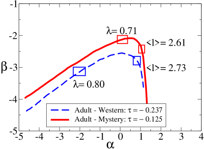
Figure 8: (color online) By tuning the two exponents $\alpha$ and $\beta$ one can construct a synthetic multiplex network which reproduces some of the structural properties of real-world system. The solid red line and the dashed blue line indicate, respectively, all the $(\alpha,\beta)$ pairs which produce multiplex networks whose inter-layer degree correlation coefficient is compatible with that observed in the Adult-Mystery ($\tau=-0.125$) and in the Adult-Western ($\tau=-0.237$) multiplex networks constructed from the IMDB data set (see Ref. Nicosia2014_corr ). The four boxes highlight the regions of the $\alpha$-$\beta$ plane in which either the characteristic path length $\langle{l}\rangle$ or the multiplex interdependence $\lambda$ are also similar to those measured on the Adult-Mystery and on the Adult-Western multiplexes.

IX Model calibration

Here we discuss the possibility of calibrating the non-linear preferential attachment model defined in Eq. (3), i.e. of choosing appropriate values of $\alpha$ and $\beta$, in order to reproduce some of the structural properties of a real-world multiplex network. As an example, we consider two 2-layer multiplex networks constructed from the IMDB costarring multi-layer network data set described in Ref. Nicosia2014_corr . In this data set, each layer corresponds to a different movie genre. The first multiplex consists of the nodes (actors) who have acted both in Adult and in Western movies, while the second one includes actors who have starred both in Adult and Mystery movies. Both systems are characterized by negative inter-layer degree correlations ($\tau=-0.237$ and $\tau=-0.125$, respectively). Let us now imagine that we want to set the values of $\alpha$ and $\beta$ in order to construct a synthetic network having the same inter-layer degree correlation pattern of each of the two multiplexes.

In Fig. 8 we report the curves in the $\alpha$-$\beta$ plane corresponding to the values of $\tau$ measured in the Adult-Western and in the Adult-Mystery multiplexes. All the points of the solid red curve are pairs of values $(\alpha,\beta)$ which produce a 2-layer multiplex with $\tau=-0.125$ (Adult-Mystery), while the pairs $(\alpha,\beta)$ indicated by the dashed blue line correspond to $\tau=-0.237$ (Adult-Western). We notice that each of these pairs of parameters produces a synthetic multiplex network having exaclty the same value of $\tau$, but in general different values of characteristic path length $\langle{l}\rangle$ and interdependence $\lambda$. In the same plot we show, for each network, the range of values which guarantee, respectively, a value of $\langle{l}\rangle$ or a value of $\lambda$ compatible with those observed in the real multiplexes. This example shows that, despite being elegant and analytically solvable, the non-linear attachment model cannot reproduce, at the same time, all the structural properties of real-world networks. This fact suggests that the preferential attachment mechanism is just one among several ingredients responsible for the formation of multiplex networks.

X General models for $M$ layers

The model defined in Eq. (2) and Eq. (3) can be generalized to the case of multiplexes with $M$ layers in at least three different ways. We review them in the following, and for the first two generalization we also give a sketch of the the derivation of the conditions for condensation.

X.1 One vs. All

A simple extension would be to consider an attaching function

$$f^{a}(\vec{\bm{k}})=(k^{[a]})^{\alpha}\prod_{b\neq a}(k^{[b]})^{\beta}$$ (35)

which says that the probability for a new node to attach on layer $a$ to a node having degree $k^{[a]}$ depends on the $\alpha-$ power of $k^{[a]}$ and on the product of the $\beta-$powers of the degrees of the same node at the other layers $b\neq a$. In this case, each layer can either compete with all the others ($\beta<0$) or cooperate with all of them ($\beta>0$), and the behavior of any two layers will be exactly the same of that studied in the previous Sections.

Following a similar approach used to determine the condensation phase diagram for the model of two layers, it is easy to show that the condensation occurs in a multiplex of $M$ layers satisfying the attachment rule given by Eq. (35) under the following conditions

$$\alpha>1,\ \beta<0~{}~{}~{}~{}~{}~{}\mbox{or}~{}~{}~{}~{}~{}~{}~{}~{}\alpha+\beta(M-1)>1,\ \beta>0.$$ (36)

In the case $\beta<0$ and $\alpha>1$ there are $M$ nodes in which the condensation occurs, exactly one in each of the $M$ layers. Each of these condensed nodes has degree $k^{[c]}\simeq t$ in exactly one layer (say layer $c$), while its degree on all the other layers is equal to $m$. Instead for $\beta>0$ and $\alpha+\beta(M-1)>1$ the condensation occurs on a single node that has degree $k^{[c]}\simeq t$ in all the layers of the multiplex.

X.2 Two groups of layers

Another possible extension of Eq. (3) to the case of $M$ layers considers layers divided into two groups, say $\Gamma_{1}$ and $\Gamma_{2}$ . We denote by $\Gamma(a)$ the group of layers to which layer $a$ belongs, and by $M_{1},M_{2}$ their cardinality $M_{1}=|\Gamma_{1}|$ and $M_{2}=|\Gamma_{2}|$. We define the attaching function:

$$f^{[a]}(\vec{\bm{k}})=\prod_{b:\Gamma(b)=\Gamma(a)}\!\!\!\!\!(k^{[b]})^{\alpha}\prod_{b:\Gamma(b)\neq\Gamma(a)}\!\!\!\!\!(k^{[b]})^{\beta}$$ (37)

meaning that the probability for a new node to connect on layer $a$ with a node of degree $k^{[a]}$ depends on the product of the $\alpha$-power of the degrees of the destination node at all layers belonging to the same group of layer $a$ multiplied by the product of the $\beta-$powers of the degrees of the destination node at all layers belonging to the other group. Also in this case the dynamics of pairwise relationships between layers belonging to different groups is similar to that observed in the 2-layer case discussed in the previous Sections. Though, the phase diagram is not exactly the same. In fact, the condensation could occur either only on the layers belonging to $\Gamma_{1}$, or only on the layers belonging to $\Gamma_{2}$ or on all the $M$ layers at the same time.

Following a similar approach used to determine the condensation phase diagram for the model of two layers, it is possible to show that the condensation occurs in a multiplex of $M$ layers satisfying the attachment rule given by Eq. (37) under the following conditions

$$\alpha M_{1}>1,\ \beta<0\quad\mbox{or}$$

$$\alpha M_{2}>1,\ \beta<0\quad\mbox{or}$$

$$\xi=\alpha(M_{1}^{2}+M_{2}^{2})+2\beta M_{1}M_{2}>2,\ \beta>0.\quad$$ (38)

In the case $\beta<0$ and $\alpha M_{1}>1$ there is a node in which the condensation occurs. This node has all the degrees in layers $c\in\Gamma_{1}$ given by $k^{[c]}\simeq t$. Similarly for $\beta<0$ one node becomes the condensate in layers $c\in\Gamma_{2}$ if $\alpha M_{2}>1$. If both $\alpha M_{1}>1$ and $\alpha M_{2}>1$ these two nodes where the condensation occurs coexist in the multiplex and are distinct. Instead for $\beta>0$ and $\xi>2$ the condensation occurs on a single node that have all the degrees $k^{[a]}\simeq t$ in every layer $a$.

X.3 More complex layer interconnections

Finally, we consider the case in which the degree of a node at each single layer might interact with the degree of the same node at any other layer by means of a power $\alpha$ or $\beta$. We define a $M\times M$ interaction matrix $\mathcal{C}=\{c_{a,b}\}$, such that $c_{a,b}=+1$ if layer $a$ interacts with layer $b$ through the exponent $\alpha$, while $c_{a,b}=-1$ if $a$ interacts with $b$ through the exponent $\beta$. Notice that in general $c_{a,b}\neq c_{b,a}$, i.e. $\mathcal{C}$ is not necessarily symmetric. In this case the attaching function reads:

$$f^{a}(\vec{\bm{k}})=\prod_{b:c_{a,b}=1}(k^{[b]})^{\alpha}\prod_{b:c_{a,b}=-1}(k^{[b]})^{\beta}$$ (39)

This model is very general and allows a pretty rich interplay between the degree distributions of the $M$ layers. In this case the conditions for condensation depend on the structure of the interconnection matrix $\mathcal{C}$, and the derivation is left as a future work.

XI Conclusions

In this Article we have introduced a general class of non-linear models to grow multiplexes which display a rich variety of behaviors, including the appearance of positive, null and negative inter-layer degree correlations and the transition to a condensed phase. We have shown that the model is highly sensitive to stochasticity, so that the mean-field approach, which has been fundamental to study growth processes on single-layer networks, fails to give account for some of its most interesting properties. Conversely, the solution of the master equation of the system gives some general theoretical insights which will certainly prove to be a useful guide in the exploration of real-world multiplex networks.

We would like to stress the fact that the class of growth models proposed in this work includes only some of the ingredients which might be responsible for the formation and evolution of multi-layer networks. As a matter of fact, real networked systems rarely evolve only by the addition of new nodes and edges at discrete time-steps. Depending on the structure and function of the multiplex system under study, nodes can also disappear and re-join the network again, with a different number of edges on each layer, and edges might be rewired, severed and re-created, sometimes according to the state of some dynamical processes occurring on the network. Also, the arrival and departure of nodes and the creation and rewiring of edges might be affected by different levels of topological and temporal correlations. All these ingredients should be taken into account for a more accurate modelling of real-world multiplex networks, and this will certainly be the subject of future research in this novel field of network science. Nevertheless we believe that, despite the few simplifying assumptions introduced to make the model analytically tractable, the present work clearly points out that multiplex networks are indeed characterized by new, additional and somehow unexpected levels of complexity, and that the multiplex perspective might reveal interesting aspects of real-world complex systems which have remained unnoticed until now.

Appendix A Inter-layer correlations

A.1 Coefficients to quantify inter-layer degree correlations

To detect and quantify the presence of inter–layer degree correlations we have evaluated the Pearson’s linear correlation coefficient $r$, the Spearman rank correlation coefficient $\rho$ and the Kendall’s $\tau$ rank correlation coefficient of the degree distributions at the two layers. If we denote as $k_{i}$ and $q_{i}$ the degrees of node $i$ respectively at layer $1$ and layer $2$, the Pearson’s correlation coefficient of the two degree sequences is defined as:

$$r=\frac{\langle{kq}\rangle-\langle{k}\rangle\langle{q}\rangle}{\sigma_{k}\sigma_{q}}$$ (A-40)

where the averages are taken over all the nodes in each layer, and the $\sigma_{\bullet}$ are the corresponding standard deviations. Similarly, if we denote by $r(k_{i})$ the rank of the degree of node $i$ on the first layer, and by $r(q_{i})$ the rank of the degree of node $i$ on the second layer, the Spearman’s correlation coefficient is defined as:

$$\rho=\frac{\sum_{i}\left(r(k_{i})-\overline{r(k)}\right)\left(r(q_{i})-\overline{r(q)}\right)}{\sqrt{\sum_{i}\left(r(k_{i})-\overline{r(k)}\right)^{2}\sum_{i}\left(r(q_{i})-\overline{r(q)}\right)^{2}}}$$ (A-41)

where $\overline{r(k)}$ and $\overline{r(q)}$ are the averages respectively at layer $1$ and layer $2$.

If we consider node $i=(i^{[1]},i^{[2]})$ and $j=(j^{[1]},j^{[2]})$ and we call $r(\cdot)$ the ranking induced at each layer by the degree sequence, we say that $(i,j)$ is a concordant pair with respect to $r(\cdot)$ if the ranks of the two nodes agree, i.e. if both $r(i^{[1]})>r(j^{[1]})$ and $r(i^{[2]})>r(j^{[2]})$ or both $r(i^{[1]})<r(j^{[1]})$ and $r(i^{[2]})<r(j^{[2]})$. If a pair of nodes is not concordant, then it is said discordant. The Kendall’s $\tau$ coefficient measures the correlation between two rankings by looking at concordant and discordant pairs:

$$\tau=\frac{n_{c}-n_{d}}{\sqrt{(n_{0}-n_{1})(n_{0}-n_{2})}}$$ (A-42)

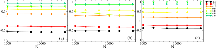
Figure A-1: (color online) In the three panels we show the value of the Kendall’s $\tau$ correlation coefficient as a function of the size $N$ of the multiplex, respectively for (a) $alpha=-1.0$, (b) $\alpha=0.0$ and (c) $\alpha=1.0$, and several values of $\beta$. Notice that the value of $\tau$ does not depend on $N$, meaning that the shape of region $-_{b}$ in Fig. 4(c) is not due to the finite size of the network.

where $n_{c}$ is the number of concordant pairs, $n_{d}$ is the number of discordant pairs, and $n_{0}=1/2N(N-1)$ is the total possible number of pairs in a set of $N$ elements. The terms $n_{1}$ and $n_{2}$ account for the presence of rank degeneracies. In particular, let us suppose that the first ranking has $m$ tied groups, i.e. $m$ sets of elements such as all the elements in one of this set have the same rank. If we call $u_{i}$ the number of nodes in the $i^{\text{t}h}$ tied group, then $n_{1}$ is defined as:

$$n_{1}=\sum_{i=1}^{m}\frac{1}{2}u_{i}(u_{i}-1).$$

Similarly, $n_{2}$ is defined as follows:

$$n_{2}=\sum_{j=1}^{n}\frac{1}{2}v_{j}(v_{j}-1)$$

where we have made the assumption that the second ranking has $n$ tied groups, and that the $j^{\text{t}h}$ tied group has $v_{j}$ elements.

The Kendall’s $\tau$ coefficient is equal to $1$ when the rankings induced by the degree sequence at each layer are perfectly concordant, while $\tau=-1$ if one of the two rankings is exactly the opposite of the other.

A.2 Pearson’s coefficient in the non-condensed phase

Using the master equation we can derive several relations between the moment of the degree distribution at long times. In particular it can be shown that for $m=1$ we have

$$\displaystyle\left\langle{k^{r}q^{s}}\right\rangle =C+\left\langle{(k+1)^{r}k^{\alpha}q^{s+\beta}}\right\rangle-\left\langle{k^{r+\alpha}q^{s+\beta}}\right\rangle$$ (A-43)

$$+\left\langle{(q+1)^{s}q^{\alpha}k^{r+\beta}}\right\rangle-\left\langle{q^{s+\alpha}k^{r+\beta}}\right\rangle.$$

In particular we have,

$$C\left\langle{k^{2}}\right\rangle=2C+2\langle{k^{1+\alpha}q^{\beta}}\rangle,~{}~{}~{}~{}~{}~{}~{}~{}~{}~{}~{}~{}~{}C\left\langle{kq}\right\rangle=2\left\langle{k^{\alpha}q^{1+\beta}}\right\rangle+C.$$ (A-44)

Therefore the Pearson’s linear coefficient $r$, defined as

$$r=\frac{\left\langle{kq}\right\rangle-\left\langle{k}\right\rangle\left\langle{q}\right\rangle}{\sigma_{k}\sigma_{q}}$$ (A-45)

with $\sigma_{k}^{2}=\left\langle{k^{2}}\right\rangle-\left\langle{k}\right\rangle^{2}$ can be also written as

$$r=\frac{\left\langle{k^{\alpha}q^{1+\beta}}\right\rangle-3/2\left\langle{k^{\alpha}q^{\beta}}\right\rangle}{\left\langle{k^{1+\alpha}q^{\beta}}\right\rangle-\left\langle{k^{\alpha}q^{\beta}}\right\rangle}.$$ (A-46)

Appendix B Stability of negative inter-layer correlations

It is interesting to investigate whether the existence of two sub-regions in the phase diagram of $\tau$ for $\beta<0$ (see Fig. 4(c) in the main text) is indeed due to finite-size effects or not. To this aim, we computed $\tau$ for networks whose size varied across three orders of magnitude. The results are reported in Fig. A-1, for different values of $\alpha$ and $\beta$. As made clear by the figures, the values of $\tau$ measured for a certain pair $(\alpha,\beta)$ do not depend on the size of the multiplex, and therefore the shape of the region $-_{b}$ is not an artifact due to finite size effects.

References

- (1) A. Cardillo et al., Sci. Rep. 3, 1344 (2013).
- (2) A. Cardillo et al., Eur. Phys. J. Spec. Top. 215, 23-33 (2013).
- (3) F. Battiston, V. Nicosia and V. Latora, Phys. Rev. E 89, 032804 (2014).
- (4) M. Szell, R. Lambiotte, S. Thurner, Proc. Natl. Acad. Sci., USA, 107, 13636 (2010).
- (5) G. Bianconi, Phys. Rev. E 87, 062806 (2013).
- (6) M. Kivela, et al, arXiv:1309.7233 (2013).
- (7) M. De Domenico et al., Phys. Rev. X 3, 041022 (2013).
- (8) V. Nicosia, V. Latora, arxiv:1403.1546 (2014).
- (9) V. Nicosia, G. Bianconi, V. Latora and M. Barthelemy, Phys. Rev. Lett. 111, 058701 (2013).
- (10) J, Y. Kim and K.-I. Goh, Phys. Rev. Lett. 111, 058702 (2013).
- (11) A. Halu, S. Mukherjee, G. Bianconi, Phys. Rev. E 89, 012806 (2014).
- (12) S.V. Buldyrev, et al. Nature 464, 1025-1028 (2010).
- (13) D. Cellai, E. López, J. Zhou, J. P. Gleeson, and G. Bianconi, Phys. Rev. E 88, 052811 (2013).
- (14) G. J. Baxter, S. N. Dorogovtsev, J. F. F. Mendes, D. Cellai, arXiv:1312.3814 (2013).
- (15) B. Min, S. D. Yi, K.-M. Lee, K.-I. Goh, arXiv:1307.1253 (2013).
- (16) G. Bianconi, S. N. Dorogovtsev, arXiv:1402.0218 (2014).
- (17) S. Gómez et al., Phys. Rev. Lett. 110, 028701 (2013).
- (18) A. Solé-Ribalta et al., Phys. Rev. E 88, 032807 (2013)
- (19) M. De Domenico, A. Sole, S. Gomez, A. Arenas, arxiv:1306.0519 (2013)
- (20) A. Halu, R. J. Mondragon, P. Panzarasa, G. Bianconi, PLoS ONE 8(10): e78293 (2013).
- (21) A. Saumell-Mendiola, M. Á. Serrano and M. Boguñá, Phys. Rev. E 86, 026106 (2012).
- (22) C. Granell, S. Gomez, A. Arenas, Phys. Rev. Lett. 111 128701 (2013).
- (23) B. Min, K.-I. Goh, arXiv:1307.2967 (2013).
- (24) E. Cozzo, R. A. Ba os, S. Meloni, Y. Moreno, Phys. Rev. E 88, 050801R (2013).
- (25) R.G. Morris, M. Barthelemy, Phys. Rev. Lett. 109, 128703 (2012).
- (26) R.G. Morris, M. Barthelemy, Scientific Reports 3:2764 (2013).
- (27) J. Gomez-Gardeñes, I. Reinares, A. Arenas and L. M. Floria, Sci. Rep. 2, 620 (2012).
- (28) L.-L. Jiang, M. Perc, Sci. Rep. 3, 2483 (2013).
- (29) Z. Wang, A. Szolnoki, M. Perc, Sci. Rep. 3, 2470 (2013).
- (30) M. Li, R.-R. Liu, C.-X. Jia, and B.-H. Wang, New Jour- nal of Physics 15, 093013 (2013).
- (31) Y. Hu, D. Zhou, R. Zhang, Z. Han, and S. Havlin, Phys. Rev. E 88, 052805 (2013).
- (32) R. Parshani, C. Rozenblat, D. Ietri, C. Ducruet and S. Havlin, EPL – Europhys. Lett. 92, 68002 (2010).
- (33) K.-M. Lee, J. Y. Kim, W. kuk Cho, K.-I. Goh and I.-M. Kim, New J. Phys. 14, 033027 (2012).
- (34) L. D. Valdez, P. A. Macri, H. E. Stanley, L. A. Braunstein, Phys. Rev. E 88, 050803(R) (2013).
- (35) P. L. Krapivsky, S. Redner, and F. Leyvraz Phys. Rev. Lett. 85, 4629 (2000).
- (36) R. Albert, H. Jeong and A.-L. Barabasi, Nature 401, 130–131 (1999).
- (37) S. N. Dorogovtsev and J. F. F. Mendes, Evolution of networks: From biological nets to the Internet and WWW (Oxford,Oxford University Press, 2003)
- (38) B. Derrida, H. Flyvbjerg J. Phys. A 20, 5273 (1987).
- (39) R. Guimera, L.A.N. Amaral, J. Stat. Mech.-Theory Exp., art. no. P02001 (2005)
- (40) R. Guimera, L.A.N. Amaral, Nature 433 (2005) 895.