On Thermodynamics of $2d$ Black Holes in Brane Inflationary Potentials

Abstract

Inspired from the inflation brane world cosmology, we study the thermodynamics of a black hole solution in two dimensional dilaton gravity with an arctangent potential background. We first derive the two dimensional black hole geometry, then we examine its asymptotic behaviors. More precisely, we find that such behaviors exhibit properties appearing in some known cases including the Anti de Sitter and the Schwarzchild black holes. Using the complex path method, we compute the Hawking radiation. The entropy function can be related to the value of the potential at the horizon.

KeyWords: Two dimensional dilaton gravity, Two dimensional black holes and inflation brane world cosmology.

1 Introduction

In the last years, the black hole physics has received an increasing attention in the context of supergravity theories embedded in superstrings and M-theory compactified on Calabi-Yau manifolds[1-8]. A particular emphasis has placed on the study of extremal black solutions in various dimensions. This concerns the attractors of extremal black holes and branes. In this way, the corresponding effective potentials and entropy functions have been computed in terms of the U-duality black brane charge invariants [9].

More recently, a special effort has been devoted to study the black hole solutions in two-dimensional models of the dilaton gravity [10, 11, 12, 13]. This black hole solution has been subject to some interest not only because of its connection with the conformal field theories but also from its connection with the cosmological models embedded in heterotic M-theory theory compactification in the presence of the dilaton coupling functions [14, 15]. In such models, the Bekenstein-Hawking entropy has been investigated and explicitly calculated. The black hole thermodynamics in two dimensional dilatonic models have been also studied by several investigation groups[16, 17, 18, 19]. It has been shown, in many places, that the black hole thermodynamics can open gates to understand the quantum features of gravity theory. It is possible to explore such thermodynamic properties to study certain field theory models using recent string theory technics including AdS/CFT conjecture.

On the other hand, the F(R)-gravity theories, in the presence of a scalar field, have been extensively studied in the connection with cosmological models embedded in superstring models and M-theory[20, 21, 22]. In particular, a new F(R)-gravity theory with a Lagrangian density involving an arctangent function has been studied in [23]. The corresponding static solutions and the potential of the scalar field have been obtained, showing a good agrement with the PLANCK data.

The aim of this work is to contribute to these activities by presenting a black hole solultion in two dimensional dilaton gravity in the presence of an inflationary potential. More precisely, we consider an arctangent potential background, explored in the brane world cosmology, to build a two dimensional black hole solution. Up to some limit conditions, it has been shown that this black hole geometry recovers some known results, including the Schwarzchild and Anti de Sitter black holes. Using the complex path analysis, the Hawking radiation is computed and commented in terms of known black hole solutions. Then we calculate the entropy function. This function can be related to the value of the potential at the horizon.

2 Two dimensional black hole in brane inflationary potential

In this section, we study two dimensional black hole solutions in the presence of an effective potential used in brane world

To get two singular two-dimensional dilatonic black hole solutions, one should first start with the most general lagrangian involved in the dilatonic gravity in [24]

$$\mathcal{L}=\sqrt{-g}(D(\phi)R+G(\phi)(\nabla\phi)^{2}+H(\phi)).$$ (2.1)

Then, one performs the following conformal transformation

$$g_{\alpha\beta}\rightarrow e^{2\sigma(\phi)g_{\alpha\beta}}$$ (2.2)

with

$$\frac{d\sigma}{d\phi}\frac{dD}{d\phi}=-\frac{1}{4}G(\phi).$$ (2.3)

In fact, the kinetic term $G(\phi)$ can be absorbed in the redefinition of the $D(\phi)$ function. Indeed, redefining the potential as $V(\phi)=e^{2\sigma(\phi)}H(\phi)$, and transforming the kinetic term, one gets the action appearing in [24]

$$\mathcal{S}=\int d^{2}x\sqrt{-g}(V(\phi)+D(\phi)R).$$ (2.4)

It is worth noting that the field equation for the scalar field $\phi$ obtained from this action does not contain derivative terms. In fact, this should be equivalent to the action involving the higher derivative with only the gravitational field namely [25]

$$\mathcal{S}_{HD}=\int d^{2}x\sqrt{-g}\mathcal{F}(R)$$ (2.5)

It turns out that the lagrangian (2.1) can be extended by introducing $N$ conformally coupled scalar fields $f_{i}$ [40]

$$\mathcal{L}=\sqrt{-g}(D(\phi)R+G(\phi)(\nabla\phi)^{2}+H(\phi))-\frac{1}{2}\sum_{i=1}^{N}(\nabla f_{i})^{2}.$$ (2.6)

However, the corresponding equations of motion are not easy to deal with. For this reason, we consider here the simplest case without conformal coupling matter fields. The general study might be examined in future works using sophisticated numerical analysis.

In connection with the higher dimensional theories, this action could be obtained from M-theory on nine dimensional compact manifolds. Indeed, within heterotic M-theory framework, the internal space can be identified with the Calabi-You fourfolds fibred by the orbifold $S^{1}/Z_{2}$ obtained by implementing the $Z_{2}$ action on the circle coordinate. In this way, the corresponding models can be derived from a three dimensional heterotic M-theory with orbifold data [26]. In the heterotic M-theory, the models associated with this action can be controlled by the $V(\phi)$ and $D(\phi)$ functions depending on the scalar field known by the dilaton in string theory and related models.

Assuming that this action can be obtained from the superstring compactification down to two dimensions and varying it with respect to the dilaton scalar field, one gets

$$-\sqrt{-g}\frac{\partial V}{\partial\phi}(\phi)=\frac{\partial D}{\partial\phi}(\phi)\sqrt{-g}R.$$ (2.7)

where $R_{\alpha\beta}=g_{\alpha\beta}\frac{R}{2}$. However, the variation with respect to the metric tensor yields

$$V(\phi)g_{\alpha\beta}=2(\nabla^{2}g_{\alpha\beta}-\nabla_{\alpha}\nabla_{\beta})D(\phi).$$ (2.8)

In what follows, we discuss a two-dimensional dilatonic black hole in a special background based on a potential explored in the inflationary brane physics. Precisely, we consider a spheric symmetric static solution, in the Schwarzschild like gauge, given by

$$ds^{2}=-f(r)dt^{2}+\frac{1}{f(r)}dr^{2},$$ (2.9)

where $f(r)$ is a scalar function specified later one in terms of the inflationary cosmological date including the potential. This metric can be obtained generally from a $d$ dimensional static spherically symmetric solution

$$ds^{2}=-f(r)dt^{2}+\frac{1}{f(r)}dr^{2}+r^{2}d\Omega^{2}_{d-2}$$ (2.10)

using the compactification on the $(d-2)$-dimensional sphere.

The metric function $f(r)$ is determined by fixing the $V(\phi)$ and $D(\phi)$ functions. Indeed, we take a particular value of the dilaton scalar field given $D(\phi)=\frac{1}{\phi}$. The above equations can be reduced to

$$\frac{\partial V}{\partial\phi}(\phi)=\frac{1}{\phi^{2}}R$$ (2.11)

together with

$$g_{\alpha\beta}V(\phi)=2(g_{\alpha\beta}\nabla^{2}-\nabla_{\alpha}\nabla_{\beta})\frac{1}{\phi}.$$ (2.12)

Technical calculations give the following equations

$$\phi^{3}V(\phi)+2f\phi\phi^{{}^{\prime\prime}}-4f\phi^{{}^{\prime}2}+f^{{}^{\prime}}\phi\phi^{{}^{\prime}}=0$$

$$\phi^{2}V(\phi)+f^{{}^{\prime}}\phi^{{}^{\prime}}=0$$ (2.13)

$$\frac{\partial V}{\partial\phi}(\phi)+\frac{1}{\phi^{2}}(f^{{}^{\prime\prime}})=0.$$

Having fixed the $D(\phi)$ function, the model will depend now only on the potential form. It turns out that there are many physical potentials incorporated in string theory and related models including M and F-theories moving on orbifold fixed spaces [26]. Such potentials have been used in the moduli stabilization in stringy cosmological models. In fact, the scalar potential shape turns out to be essential in the elaboration of stringy inflationary models. The well studied models are the chaotic inflation potential reported in [27, 28] and the minimal supersymmetric standard model inflation discussed in [29, 30]. Besides such examples, there are several other models which have been also investigated in the literature.

To keep contact with the brane inflationary models, we will consider a cosmological potential satisfying the limiting curvature condition proposed in [31]. This inflationary potential takes the form

$$V(\phi)=\lambda\arctan(\phi^{2}),$$ (2.14)

where $\lambda$ is a constant. This constant represents the large field approximation. It is worth noting that this potential has many nice cosmological properties[32]. In particular, for very small values of the dilaton scalar field, it behaves as the chaotic one. More precisely, when $\phi^{2}$ is very close to zero, at second order, a chaotic inflation scenario can be recovered [27, 28]. Moreover, the Taylor expansion at order 10 can reproduce the MSSM inflation potential studied in[29, 30].

After specifying the above functions, we are now in position to derive the associated $f(r)$ metric function producing a two dimensional black hole solution. This can be done according to the analysis presented in [35]. To present such solutions, let us first take some conditions on the dilaton field given by $\phi=\frac{1}{\alpha r}$, where $\alpha$ is a constant. After calculation, we get

$$f(r) = C-\frac{Cr}{r_{0}}+\frac{r\lambda}{\alpha}(\arctan[\alpha^{2}r_{0}^{2}]-\arctan[\alpha^{2}r^{2}])$$ (2.15)

$$+ \frac{\lambda}{\alpha\sqrt{2}}(\arctan[1+\alpha\sqrt{2}r]-\arctan[1-\alpha\sqrt{2}r])+\frac{r\lambda}{\sqrt{2}r_{0}\alpha}(\arctan[1-\alpha\sqrt{2}r_{0}]-\arctan[1+\alpha\sqrt{2}r_{0}])$$

$$+ \frac{\lambda}{2\sqrt{2}\alpha^{2}}Log\left[\frac{1-\sqrt{2}\alpha r+\alpha^{2}r^{2}}{1+\sqrt{2}\alpha r+\alpha^{2}r^{2}}\right]+\frac{r\lambda}{2\sqrt{2}\alpha^{2}}Log\left[\frac{1+\sqrt{2}\alpha r_{0}+\alpha^{2}r_{0}^{2}}{1-\sqrt{2}\alpha r_{0}+\alpha^{2}r_{0}^{2}}\right]$$

where $r_{0}$ is the location of the black hole horizon, and $C$ is a constant of the integration, fixed later one. The computed function $f(r)$ is presented in figure 1.

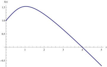
Figure 1: A plot of $f(r)$ for the values $\alpha=\lambda=C=1$, the function $f(r)$ vanishes at the horizon $r=r_{0}$.

Before going ahead, let us comment the obtained solution. In fact, we will see that the above potential can recover some known black hole solutions in two dimensions including Schwarzchild and Anti de Sitter ones. Indeed, asymptotic regions in the moduli space for either large or vanishing values of $\phi$ produce a black hole solution controlled by the following solution

$$f(r)\underset{\alpha\to 0,\infty}{\longrightarrow}C\left(1-\frac{r}{r_{0}}\right).$$ (2.16)

Such regions are defined when $\alpha$ goes to zero or infinity that mean for large or vanishing values of $\phi$. To see that, it is useful to consider the following radial variable transformation

$$r\mapsto r^{\xi}$$ (2.17)

where $\xi$ is a natural number fixed later one. Putting $\xi=2$, we can recover the Anti de Sitter metric solution. In this case, the $f(r)$ function tends to

$$f(r)=C\left(1-\frac{r^{2}}{r_{0}^{2}}\right).$$ (2.18)

Fixing again the constant of the integration to one ($C=1$) and identifying the event horizon with the cosmological constant $r_{0}^{2}=-\ell^{2}$, the above equation becomes

$$f(r)=1+\frac{r^{2}}{\ell^{2}}.$$ (2.19)

This particular value of $\xi$ reproduces the result presented in [10].
Taking $\xi=-1$, we can get the metric describing the Schwarzchild black hole. In this case, the function $f(r)$ becomes

$$f(r)=C\left(1-\frac{r_{0}}{r}\right).$$ (2.20)

As in the previous case, setting $C$ to $1$ and identifying $r_{0}$ with the mass of black hole $r_{0}=2m$, one gets

$$f(r)=1-\frac{2m}{r}.$$ (2.21)

The second comment that we should add concerns the Ricci scalar $R$. Using (2.6), the above potential produces the following Ricci scalar $R$

$$R=\frac{2\alpha\lambda r}{\alpha^{4}r^{4}+1}.$$ (2.22)

This quantity is finite for all positive values of the radial coordinate $r$. Indeed, the corresponding function is plotted below in figure 2.

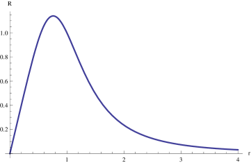
Figure 2: The curvature $R$ remains finite and positive for all $r$ from $r=0$ to $r=\infty$.

It follows from this figure that the curvature remains positive. Moreover, the Ricci scalar function $R$ has a maximum at $r=\frac{1}{\sqrt[4]{3}\alpha}$. The corresponding value is given by

$$R_{max}=\frac{1}{2}3^{3/4}\lambda.$$ (2.23)

The last comment concerns the mass of the obtained black hole. Based on the result of [32], the $\lambda$ parameter seems to behave as a mass term in the attractor mechanism, although it is fixed at infinity and not at the horizon. This observation is inspired from the analysis of the four dimensional brane inflation model associated with the potential given in (10). In this way, the scalar large value has been shown to be identified with the mass of the Schwarzchild black hole. It is recalled that the Friedmann-Robertson-Walker equation in two dimensional inflation-brane ([38]) background can be written as

$$H^{2}=\left(\frac{\dot{a}}{a}\right)^{2}=\left(\frac{\kappa}{2}\rho\right)^{2}-\frac{R+2m}{a^{2}}$$ (2.24)

where $a(t)$ is the scale factor, and where $H(t)$ is the Hubble parameter. In this equation, $\kappa$ is related to the D1-brane tension and the Planck mass. The parameter $R$ is the curvature of space given by $(\ref{19curv})$, and $m$ denotes the mass of the black hole. The dynamics can be described by a perfect fluid with a time dependent energy density $\rho=\frac{1}{2}\dot{\phi}^{2}+\lambda arctan(\phi^{2})$ and the pressure $p=\frac{1}{2}\dot{\phi}^{2}-\lambda arctan(\phi^{2})$ is the dominate energy distribution to the inflation. The dilaton field satisfies the Klein-Gordon equation

$$\ddot{\phi}-3H\dot{\phi}+\frac{2\lambda\phi}{\phi^{4}+1}=0.$$ (2.25)

In the large field approximation, the effective potential behaves like $V(\phi)\sim\lambda$. In this limit, (2.24) can be reduced to

$$H^{2}=\left(\frac{\dot{a}}{a}\right)^{2}=\left(\frac{\kappa}{2}\rho^{2}\right)^{2}-\frac{2m}{a^{2}}.$$ (2.26)

and the Klein-Gordon equation becomes

$$\ddot{\phi}-3H\dot{\phi}=0.$$ (2.27)

Solving the above equation, the expression of the dilatonic field is given by

$$\phi(t)=\phi_{\infty}+\phi_{0}\;exp(-3Ht).$$ (2.28)

Asymptotic behaviors require that $\phi_{\infty}$ should take very large values. In this limit, the dilaton field is almost constant and becomes very large when $t$ goes to infinity. In what follows, one considers the scale factor

$$a(t)=a_{0}exp(Ht).$$ (2.29)

Taking a particular geometry given by

$$H=\lambda$$ (2.30)

and using (2.29), we get the following equation

$$m(t)\sim\lambda^{2}a_{0}^{2}exp(\lambda t).$$ (2.31)

In the case where $\lambda$ takes small values, that is in the limit $\lambda t<<0$, the mass equation becomes

$$m\sim\lambda$$ (2.32)

where $a_{0}^{2}$ has been fixed to $\frac{1}{\lambda}$. This equation relates the mass of the black hole and the asymptotic value of the potential.

3 Thermodynamic properties

Having constructed the black hole solution, a particular emphasis will put on discussing its thermodynamic properties including the Hawking radiation and the entropy function. First, we compute the Hawking radiation using a method based on the complex path analysis introduced by Landau [33]. In order to derive that, it is essential to recall such a method. Assuming that $f(r)$ vanishes at $r_{0}$ and $f^{\prime}(r)$ is nonzero at $r_{0}$ and expanding it around the point $r_{0}$, one obtains

$$f(r)=f^{\prime}(r_{0})(r-r_{0})+\mathcal{O}\left[(r-r_{0})^{2}\right]\equiv\mathcal{R}(r_{0})(r-r_{0}).$$ (3.1)

To show how to get the expression of the temperature, it is useful to consider an auxiliary field $\Phi$ interacting with the above system and satisfying the Klein-Gordon equation

$$\left(\square-\frac{m_{0}^{2}}{\hbar^{2}}\right)\Phi=0.$$ (3.2)

Expanding this equation, one finds the following expression

$$-\frac{1}{f(r)}\frac{\partial^{2}\Phi}{\partial t^{2}}+\frac{\partial}{\partial r}\left(f(r)\frac{\partial\Phi}{\partial r}\right)=\frac{m_{0}^{2}}{\hbar^{2}}\Phi$$ (3.3)

To get a semiclassical wave function, one should consider the following standard ansatz

$$\Phi(r,t)=e^{\frac{i}{\hbar}\mathcal{S}(r,t)}.$$ (3.4)

This ansatz leads to

$$-\frac{1}{f(r)}\left(\frac{\partial\mathcal{S}}{\partial t}\right)^{2}+f(r)\left(\frac{\partial\mathcal{S}}{\partial r}\right)^{2}+m_{0}^{2}-\frac{i}{\hbar}\left[\frac{1}{f(r)}\frac{\partial^{2}\mathcal{S}}{\partial t^{2}}-f(r)\frac{\partial^{2}\mathcal{S}}{\partial r^{2}}-\frac{df(r)}{dr}\frac{\partial\mathcal{S}}{\partial r}\right]=0.$$ (3.5)

Expanding $\mathcal{S}$ in a power series of $\hbar/i$ and neglecting the higher orders, one obtains

$$\mathcal{S}_{0}=-\mathcal{E}t\pm\int\frac{dr}{f(r)}\sqrt{\mathcal{E}^{2}-m_{0}^{2}f(r)}$$ (3.6)

where $\mathcal{E}$ is a constant witch can be identified with the energy. The desired formula can be derived by taking a simple case corresponding to $m_{0}=0$. Indeed, we consider the usual saddle point method to calculate the semiclassical propagator $\mathcal{K}(z^{\prime\prime},z^{\prime})$ for a particle propagating from a spacetime point $z^{\prime\prime}(t_{1},x_{1})$ to $z^{\prime}(t_{2},x_{2})$. The propagation takes the form

$$\mathcal{K}(z^{\prime\prime},z^{\prime})=\mathcal{N}\exp\left[\frac{i}{\hbar}\mathcal{S}_{0}(z^{\prime\prime},z^{\prime})\right]$$ (3.7)

where $\mathcal{N}$ is a normalization constant and $\mathcal{S}_{0}$ reads as

$$\mathcal{S}_{0}(z^{\prime\prime},z^{\prime})=-\mathcal{E}(t_{2}-t_{1})\pm\int_{x1}^{x2}\frac{dr}{f(r)}.$$ (3.8)

To compute the amplitudes and the probabilities of the emission and the absorption at $r_{0}$, one may consider an outgoing particle at $x=x_{1}<r_{0}$. In this way, the modulus squared of the amplitude for such a particle crossing the horizon can give the probability of the emissions. Roughly, the complex analysis on the plane reveals the following expression

$$\mathcal{S}_{0}[emission]=\frac{i\pi\mathcal{E}}{\mathcal{R}(r_{0})}+\text{real part},\qquad\mathcal{S}_{0}[absorption]=-\frac{i\pi\mathcal{E}}{\mathcal{R}(r_{0})}+\text{real part}$$ (3.9)

Following [10], it has been shown that the squaring of the modulus leads to

$$P[emission]=\exp\left[\frac{-4\pi\mathcal{E}}{\mathcal{R}}\right]P[absorption]$$ (3.10)

A close inspection and a comparison with Hawking and Hartle formulation $P[emission]=e^{-\beta\mathcal{E}}P[absorption]$, gives the following expression

$$T_{H}=\beta^{-1}=\frac{|\mathcal{R}|}{4\pi}.$$ (3.11)

Using equations(3.1) and (2.15), the temperature can be written as

$$T_{H}=\frac{1}{4r_{0}\alpha^{2}}\left|-4C\alpha^{2}+\sqrt{2}\lambda\left(2arctan[1-\sqrt{2}r_{0}\alpha]-2arctan[1+\sqrt{2}r_{0}\alpha]+\log\left[\frac{1+r_{0}\alpha(\sqrt{2}+r_{0}\alpha)}{1+r_{0}\alpha(-\sqrt{2}+r_{0}\alpha)}\right]\right)\right|$$ (3.12)

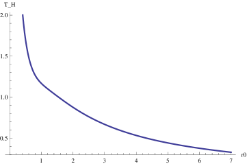
Figure 3: A plot of Hawking temperature $T_{H}$ for the values $\alpha=\lambda=C=1$

The temperature variable allows one to define new regions in the spacetime and the moduli space. Applying an appropriate approximation, we can recover some usual results. Indeed, in the region corresponding to $\alpha$ goes to infinity or zero, the above equation reduces to the following form

$$T_{H}=\frac{1}{4\pi}\left|\frac{\text{C}}{r_{0}}\right|.$$ (3.13)

It follows from this equation that the constant $C$ controls the black hole evaporation. This limiting behavior can recover the expression black hole. Identifying $r_{0}$ with the mass of the Schwarzchild black hole $r_{0}=2m$, as we made before, we obtain

$$T_{H}=\frac{1}{8\pi m}.$$ (3.14)

It is observed that for large or small values of the dilaton scalar field $\phi$, the thermodynamical behavior remains the same. This can be interpreted as a possible duality between two different regions associated with the small and large values of the dilaton scalar field $\alpha$. It looks like the strong/weak coupling duality observed in superstring theory. This observation merits an investigation. Moreover, a two dimensional version of Stefan’s law produces the total power radiated by the black hole. This can be given by the following relation

$$\mathcal{P}\sim-\frac{dm}{dt}\sim T_{H}^{2}$$ (3.15)

It is worth noting that the entropy is one of the important thermodynamic quantity of the black hole physics. Indeed, we first calculate the surface gravity $\kappa$ evaluated at the event horizon[34]. The result is

$$\kappa=-\frac{\lambda}{2}\arctan(\alpha^{2}r_{0}^{2}).$$ (3.16)

The variation of the energy takes the following form

$$\delta\epsilon=-\frac{\lambda}{2G}\arctan(\frac{1}{\alpha^{2}r_{0}^{2}})\delta\left(\frac{1}{\alpha^{2}r_{0}}\right)$$ (3.17)

The first law of the thermodynamics $\delta\epsilon=T\delta S$ produces the following entropy function

$$S=\frac{2\pi\alpha^{2}r_{0}^{2}}{G}.$$ (3.18)

The $\alpha^{2}r_{0}^{2}$ quantity denotes the value of the potential at the black hole horizon when $\alpha$ goes to zero.

4 Conclusion

In this work, we have studied a black hole solution in two dimensional dilaton gravity. To make contact with the string inflation brane world, we have dealt with a model based on an arctangent potential background. Starting from this particular potential form, we have built first a two dimensional black hole solution. Under some limit conditions, this solution recovers some known examples obtained in the literature. Using the complex path analysis, we have computed the Hawking radiation. In particular, we have considered some asymptotic behaviors reproducing the Schwarzchild black hole case. The entropy function has been also calculated and can be related to the value of the potential at the horizon.

This work comes up with many questions related to possible extended potentials. A curios question concerns the connection with string theory compactified on the Calabi-Yau manifolds producing extra scalar fields associated with the stringy moduli space. In fact, the potential used here could be extended to

$$V(\phi_{i})=\sum_{i}\lambda_{i}\arctan(\phi_{i}^{2}).$$ (4.1)

In this way, these scalar fields can be identified with the R-R B-field on 2-cycles of the Calabi-Yau manifolds. Open string field axions, appearing in the supersymmetric consistent D-brane models, can be also implemented in the discussion. Usually, the letters are related with the Peccei-Quinn symmetry in four dimensions. In connection with higher dimensions, it should be also interesting to go up by considering four dimensional models and make contact with the black hole attractor mechanism and cosmological activities [39].

Acknowledgments: AB would like to thank P. Diaz and M. Naciri for discussion on the related topics. AS is supported by the Spanish MINECO (grants FPA2009-09638 and FPA2012-35453) and DGIID-DGA (grant 2011-E24/2).

References

- [1] H. Ooguri, A. Strominger, C. Vafa, Black Hole Attractors and the Topological String, Phys. Rev. D70 (2004) 106007, hep-th/0405146.
- [2] C. Vafa, Two dimensional Yang-Mills, black holes and topological strings, hep-th/0406058.
- [3] M. Aganagic, A. Neitzke, C. Vafa, BPS Microstates and the Open Topological String Wave Function, hep-th/0504054.
- [4] A. Belhaj, P. Diaz, A. Segui, Magnetic and Electric Black Holes in Arbitrary Dimension, Phys.Rev. D80 (2009) 044015.
- [5] A. Belhaj, M. Chabab, H. El Moumni, M.B. Sedra, On non-commutative black holes and their thermodynamics in arbitrary dimension, Afr.Rev.Phys. 8 (2013) 0017.
- [6] A. Belhaj, M. Chabab, H. El Moumni, M. B. Sedra, Theromodynamics of AdS Black Holes in Arbitrary Dimensions, Chin. Phys. Lett. Vol. 29, No.10(2012)100401.
- [7] D. Kubiznak, R. B. Mann, P-V criticality of charged AdS black holes, JHEP 1207 (2012)33.
- [8] A. Belhaj, M. Chabab, L. Medari, H. El Moumni, M. B. Sedra, The Thermodynamical Behaviors of Kerr Newman AdS Black Holes, Chin.Phys.Lett. 30 (2013) 090402.
- [9] S. Ferrara, K. Hayakawa, A. Marrani, Erice Lectures on Black Holes and Attractors, arXiv:005.2498 [hep-th]. S. Bellucci, S. Ferrara, R. Kallosh, A. Marrani, Extremal Black Hole and Flux Vacua Attractors, Lect. Notes Phys. 755(2008)115-191, arXiv:0711.4547 [hep-th]. S. Bellucci, S. Ferrara, A. Marrani, A. Yeranyan, stu Black Holes Unveiled, Entropy 10(4)(2008)507-555, arXiv:0807.3503[hep-th].
- [10] D. Grumiller, W. Kummer, D.V. Vassilevich, Dilaton Gravity in Two Dimensions, Phys.Rept.369(2002)327-430, hep-th/0204253.
- [11] S. Nojiri, S. D. Odintsov, Quantum dilatonic gravity in (D = 2)-dimensions, (D = 4)-dimensions and (D = 5)-dimensions, Int.J.Mod.Phys. A16 (2001) 1015-1108.
- [12] J. A. Harvey, A. Strominger, Quantum aspects of black holes, hep-th/9209055.
- [13] D. Y. Chen, Q. Q. Jiang, X. T. Zu, Fermions tunnelling from the charged dilatonic black holes, C.Q.G. 25(2008) 205022.
- [14] D. A. Easson, Hawking radiation of non singular black holes in two dimensions, JHEP 02(2003)037.
- [15] J. Ambjorn, J. Jurkiewicz, R. Loll, Quantum Gravity, or The Art of Building Spacetime, in Approaches to Quantum Gravity, ed. D. Oriti, Cambridge University Press (2006).
- [16] D. Grumiller, An action for the exact string black hole, JHEP0505(2005)028.
- [17] D. Grumiller, R. McNees, Thermodynamics of Black Holes in Two (and Higher) Dimensions, JHEP 0704(2007)074.
- [18] A. Belhaj, K. Bilal, M. Nach, M.B. Sedra, Solutions and Thermodynamics of Noncommutative Liouville Black Hole, Int.J.Geom.Meth.Mod.Phys. 10 (2013) 1350009 .
- [19] C. Germani, G. P. Procopio, Two-dimensional Quantum Black Holes, Branes in BTZ and Holography, Phys.Rev. D74 (2006) 044012, arXiv:hep-th/0605068.
- [20] S. Nojiri, S. D. Odintsov, Unified cosmic history in modified gravity: from F(R) theory to Lorentz non-invariant models, Phys.Rept.505(2011)59-144.
- [21] R. R. Caldwell and M. Kamionkowski, Ann. Rev. Nucl. Part. Sci. 59 (2009)397.
- [22] T. P. Sotiriou and V. Faraoni, Rev. Mod. Phys. 82 (2010)451-497.
- [23] S. I. Kruglov, Modified arctan-gravity model mimicking cosmological constant, arxiv: 1310.6915.[hep-th].
- [24] T. Banks, M. O’Loughlin, Lagrangians for Two Dimensional Black Holes, Phys.Rev. D48 (1993) 698-706.
- [25] S. Naftulin, S.D. Odintsov, On higher-derivative dilatonic gravity in two dimensions, Mod.Phys.Lett.A10(1995)2071-2080.
- [26] E. J. Copeland, J. Ellison, A. Lukas, J. Roberts, Cosmological Solutions of Low-Energy Heterotic M-Theory, Phys.Rev.D73(2006)086009, hep-th/0601173.
- [27] R. Maartens, D. Wands, B. A. Bassett, I. P. C. Heard, Chaotic inflation on the brane, hep-ph/9912464.
- [28] E. Papantonopoulos, V. Zamarias, Chaotic Inflation on the Brane with Induced Gravity, JCAP 10 (2004) 001, gr-qc/0403090.
- [29] R. Allahverdi, J. Garcia-Bellido, K. Enqvist, A. Mazumdar, Gauge Invariant MSSM Inflaton, hep-ph/0605035.
- [30] D. H. Lyth, MSSM Inflation, hep-ph/0605283.
- [31] M. Trodden, V.F. Mukhanov, R.H. Brandenberger, A nonsingular two-dimensional black hole, Phys. Lett. B 316 (1993) 483 hep-th/9305111.
- [32] A. Belhaj, P. Diaz, M. Naciri, A. Segui, On Brane inflation potentials and black hole attractors, Int. J. Mod. Phys. D17 (2008) 911-920.
- [33] R. H. Landau, Quantum mechanics: non-relativistic theory, Pergamon Press, New York (1977).
- [34] R. M. Wald, General Relativity, Chicago Univ. Press, Chicago: 1984.
- [35] J. B. Hartle, S.W. Hawking, Path integral derivation of black hole radiance, Phys. Rev. D13 (1976) 2188.
- [36] J. R. B, Mann, Conservation Laws and 2D black holes in dilaton gravity, hep-ph/9206044.
- [37] J. Gegenberg, G. Kunstatter, D. L. Martinez, Observables for two dimensional black holes, gr-qc/9408015.
- [38] H. Kodama, A. Ishibashi, O. Seto, Brane World Cosmology-Gauge, Invariant Formalism for Perturbation, Phys. Rev. D62 (2000) 064022, hep-th/0004160.
- [39] T. Kadoyoshi, S. Nojiri, S. D. Odintsov, Four-dimensional cosmology from dilaton coupled quantum matter in two dimensions, Phys.Lett.B425 (1998) 255-264.
- [40] Mariano Cadoni, Trace anomaly and the Hawking effect in generic two-dimensional dilaton gravity theories, Phys. Rev. D53 (1996) 4413-4420 , gr-qc/9510012.