Magnetic Fields in Low-Mass Stars:
An Overview of Observational Biases

Abstract

Stellar magnetic dynamos are driven by rotation, rapidly rotating stars produce stronger magnetic fields than slowly rotating stars do. The Zeeman effect is the most important indicator of magnetic fields, but Zeeman broadening must be disentangled from other broadening mechanisms, mainly rotation. The relations between rotation and magnetic field generation, between Doppler and Zeeman line broadening, and between rotation, stellar radius, and angular momentum evolution introduce several observational biases that affect our picture of stellar magnetism. In this overview, a few of these relations are explicitly shown, and the currently known distribution of field measurements is presented.

1 Introduction

An important difference between massive and low-mass stars is the presence of an outer convection zone. In this article, we distinguish between high- and low-mass stars on the basis of the presence of an outer convective zone; high-mass stars have no outer convective envelopes. While they may have convective cores, radiative energy transport dominates in the outer zones of these stars. Because dissipation timescales are long, strong magnetic fields may survive there, but fields are not generated, and fields that may be generated in the core find no easy way to the surface.

Low-mass stars, on the other hand, have outer convective envelopes in which magnetic fields decay within only a few decades or centuries [Chabrier & Küker, 2006, (Chabrier & Küker, 2006)], and where motion of ionized particles apparently manage to generate strong magnetic fields as for example in the Sun. The efficiency of magnetic field generation through a dynamo process depends on several conditions, but the details of these are not well known [Charbonneau, 2010, (e.g., Charbonneau, 2010)]. The Sun is one anchor for our models of stellar dynamos. It is probably a fairly common representative of its type [Basri et al., 2013, (Basri et al., 2013)], but we know many stars that are a lot younger and more active. These stars produce orders of magnitude more non-thermal radiation (activity). The reason for this is probably their faster rotation leading to enhanced dynamo action powering non-thermal heating of the chromosphere and corona.

Observations of magnetic fields in stars other than the Sun require relatively high data quality. More important, the signatures of magnetic fields must be disentangled from other effects, which is often difficult because the characteristic properties of low-mass stars evolve in time (and differently for different stellar masses). In this article, I introduce the main characters important for spectroscopic measurements of magnetic fields and their interpretation, and I present the currently known distribution of field measurement using different techniques. A more comprehensive review about observations of low-mass star magnetic fields can be found in [Reiners, 2012, Reiners (2012)] where the data used here are also presented.

2 Cast of Characters

Four main characters are conspiring in our picture of stellar dynamos and their spectroscopic observations. They are the following:

2.1 Zeeman

  

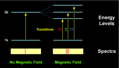
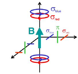
Figure 1: Simplified Zeeman splitting mechanism. The upper energy level is split into three levels in the presence of a magnetic field (right). The three different components have different polarizations and produce very different signatures depending on the direction of observation (right).

The Zeeman effect is the most obvious and most direct consequence of the presence of a magnetic field in a star. As we know from the Sun, magnetic fields can lead to enhanced non-thermal radiation that we call activity, but only the direct detection through the Zeeman effect can show that stars other than the Sun really follow similar rules, and that other stars do indeed produce average magnetic fields orders of magnitude stronger than the Sun does.

The principle of the Zeeman effect is shown in Fig. 1. The energetic degeneracy between energy levels can be lifted by the presence of a magnetic field, which typically leads to three different groups of transitions, two $\sigma$-groups and one $\pi$-group. The groups have different polarizations and are selectively emitted into certain directions depending on the orientation of the magnetic field. The displacement of the $\sigma$-groups with respect to the non-displaced $\pi$-group is

$$\frac{\Delta\lambda}{\mathrm{m\AA}}=46.67\,g\left(\frac{\lambda_{0}}{\mathrm{\mu m}}\right)^{2}\frac{B}{\mathrm{kG}};$$ (1)

written in units of wavelength, the Zeeman effect is a function of $\lambda^{2}$. In units of velocity, the Zeeman effect can be written as

$$\frac{\Delta v}{\mathrm{ms^{-1}}}=1.4\,g\,\frac{\lambda_{0}}{\mathrm{\mu m}}\frac{B}{\mathrm{G}},$$ (2)

which still depends on wavelength. At a wavelength of $\lambda=1\,\mu$m, the typical Zeeman displacement is $\Delta v=1$ m s^-1 for a field strength of $B=1$ G.

2.2 Stokes

Figure 2: The four Stokes parameters.

The polarization states of the $\pi$- and $\sigma$-components are different. This provides great potential for the detection and measurement of magnetic fields because different polarizations can be compared with each other differentially. Individual polarization vectors, however, cannot simply be observed but need to be filtered out, e.g., by the use of polarizing beamsplitters [Tinbergen, 1996, (see, e.g., Tinbergen, 1996)]. Together with retarding waveplates, combinations of linear and circular polarizations can be observed consecutively. One possible choice for observable combinations of polarization states is defined by the so-called Stokes vectors, shown in Fig. 2. Stokes I is simply the integrated light, i.e. the sum of of the two perpendicular linear or circular components. Stokes Q and U are the differences of the two perpendicular linear polarization components, the reference frames of Q and U are rotated by $45^{\circ}$ with respect to each other. Stokes V is the difference between left- and right-handed circular polarization.

Depending on the direction of observation, the linear and circular polarization vectors carry different parts of the magnetic field information. What is worse, regions of opposite polarity produce circular polarization that can entirely cancel out each other. This is because the blue-shifted circularly polarized component of a “positive” magnetic field has exactly the same shift and amplitude as the analog component caused by a “negative” magnetic field, but the sign of that component is opposite. The sum of the two Stokes V components is therefore exactly zero. Note that this cancellation does not occur in the linearly polarized components because the direction of polarization is identical for the two $\sigma$-components. It is important to realize that the information in integrated light, Stokes I, depends on the direction of observation, too, mainly because the linearly polarized $\pi$-components are invisible if the magnetic field direction is parallel to the direction of observation.

2.3 Doppler

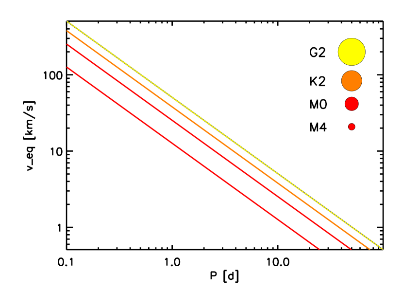
Figure 3: Equatorial Doppler velocities for four MS stars as a function of their rotation periods. The spectral types and relative sizes are shown in the upper right legend. The vertical position of the relations follows the ordering in the legend (and colors of the lines match legend colors).

In a rotating star, light emitted from the side of the star that is approaching the observer is blueshifted, and light from the other side of the star is redshifted. This leads to net broadening of spectral lines and can be used to determine the projected rotational velocity, $v\,\sin{i}$, of the star [Gray, 2008, (e.g., Gray, 2008)]. Low-mass stars as defined here (all stars with outer convective envelopes) include all stars with masses and radii between approximately 1.2 and 0.1 times the solar values, i.e., their characteristic properties vary over more than one order of magnitude. Young stars can also possess outer convective envelopes and are a lot larger than main sequence (MS) stars adding to the great variety of targets. In Fig. 3, the equatorial velocities of four different MS stars are shown as a function of their rotation periods. For example, a G2 star with a rotation period of $P=10$ d will have an equatorial velocity of $v_{\mathrm{eq}}=5$ km s^-1, but an M4 star of the same period will only show a maximum line broadening corresponding to the equatorial velocity of $v_{\mathrm{eq}}=1$ km s^-1. This difference has severe consequences for the observability of spectroscopic line diagnostics, as for example Zeeman broadening, because Zeeman broadening must be disentangled from Doppler broadening.

2.4 Rossby

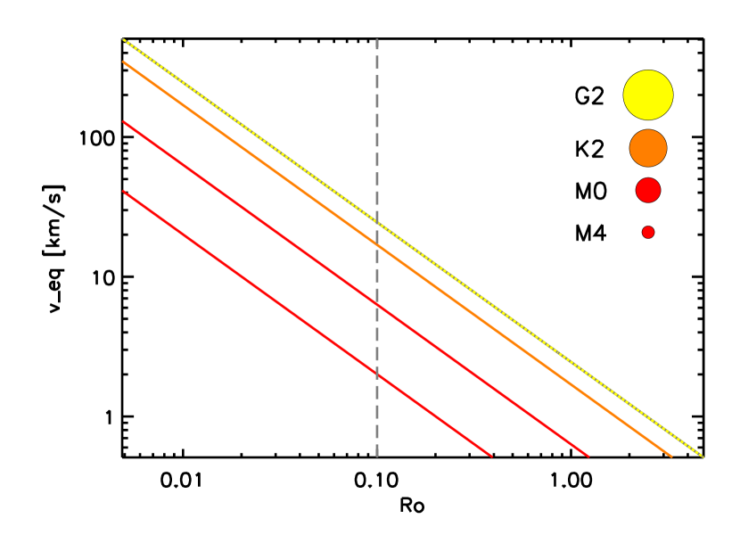
Figure 4: Equatorial Doppler velocities for four MS stars as a function of Rossby number. The spectral types and relative sizes are shown in the upper right legend. The vertical position of the relations follows the ordering in the legend (and colors of the lines match legend colors).

A prediction from Dynamo theory is that the efficiency of a convective stellar dynamo may depend on the ratio between Coriolis force and field dissipation [Ossendrijver, 2003, (e.g., Ossendrijver, 2003)]. This ratio can be expressed in terms of typical convective and rotation timescales. For the rotation timescale, an obvious choice is the rotational period. For the convective timescale, a timescale used quite often is the convective overturn time, which is defined as the typical convective velocity divided by the size of the convection zone [Durney & Latour, 1978, (Durney & Latour, 1978)]. The ratio of the two is called the Rossby number, $Ro=P/\tau_{\mathrm{conv}}$.

The convective overturn time is a slowly varying function of stellar mass, and therefore the Rossby number is mostly determined by the value of the rotation period. Nevertheless, if activity in different stars should be compared, it is often useful to use the Rossby number instead of comparing rotation periods. Figure 4 shows the equatorial velocity on the surface of a star as a function of Rossby number. It is similar as Fig. 3 but the differences in $v_{\mathrm{eq}}$ are even larger for stars of different mass because not only the radius but also the Rossby number is different.

3 Zeeman or Doppler?

                    

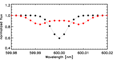
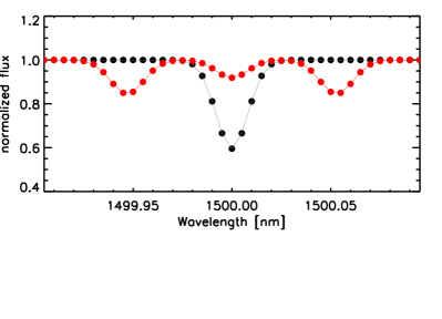
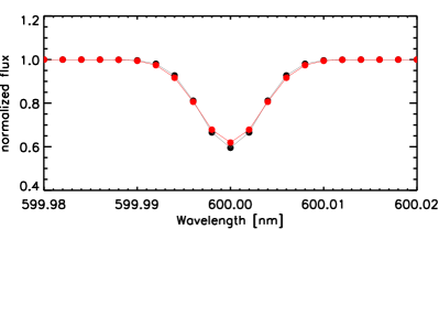
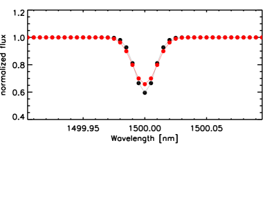
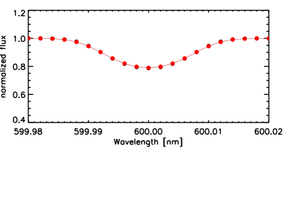
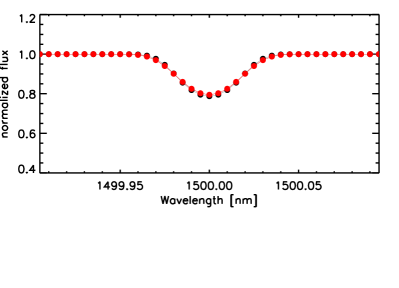
Figure 5: The effect of Zeeman broadening on a single spectral line. Left: A typical line at $\lambda=600$ nm; right: a typical line at $\lambda=1500$ nm; $g=2$ in all cases. Upper panel: Zeeman broadening in a star with an average magnetic field of $B=2000$ G (red) compared to a line with no $B=0$ G. Centre panel: Effect of a field of $B=200$ G (red) compared to zero field strength. Bottom panel: Effect of $B=200$ G observed in a star rotating at $v\,\sin{i}=5$ km s^-1.

The relation between rotation and activity is a well-established observational fact; slow rotators produce little activity, faster rotators produce more [Pizzolato et al., 2003, Wright et al., 2011, (Pizzolato et al., 2003; Wright et al., 2011)]. The ratio between activity seen in non-thermal emission and the star’s bolometric luminosity is a function of the rotation period, but it differs between different stars. For equal Rossby numbers, however, it is expected that this ratio is similar for all stars. Therefore, convective overturn times are sometimes motivated empirically by searching for the function of $\tau_{\mathrm{conv}}$ that minimizes the scatter in the activity-rotation relation [Noyes et al., 1984, Kiraga & Stepien, 2007, Wright et al., 2011, (Noyes et al., 1984; Kiraga & Stepien, 2007; Wright et al., 2011)]. A problem for the theoretical calculations of $\tau_{\mathrm{conv}}$ is that it is not obvious what definition of $\tau_{\mathrm{conv}}$ one should use – is it the convective overturn time at the bottom of the convective envelope, or the weighted mean throughout the convection zone, or something different?

Measuring a magnetic field in a rotating star requires Zeeman broadening to be a significant fraction of the total line broadening that is dominated by rotation. In slow rotators ($Ro>0.1$), the magnetic field grows with rotation, in fast rotators, the field seems to be saturated and the field does not grow further with rotation [Reiners et al., 2009, (Reiners et al., 2009)]. The ratio between Zeeman and Doppler broadening is therefore smaller in the regime of saturated dynamos.

The effect of Zeeman broadening in the presence of rotation is displayed in Fig. 5; the bottom panel of this figure shows a typical situation for a sun-like star at $Ro\approx 0.5$.

In the non-saturated part of the rotation-activity or rotation-magnetic field relation, Zeeman broadening ($\Delta v_{\mathrm{Zeeman}}$) is approximately proportional to Doppler broadening ($v_{\mathrm{eq}}$). Based on the heterogeneous sample of Zeeman measurements collected in [Reiners, 2012, Reiners (2012)], an estimate of the ratio for G dwarfs is

$$\frac{\Delta v_{\mathrm{Zeeman}}}{v_{\mathrm{eq}}}\approx 0.07\left(\frac{\lambda_{0}}{1\,\mathrm{\mu m}}\right)g.$$ (3)

This ratio is approximately valid for all stars with non-saturated activity. In more rapidly rotating stars, the ratio is smaller because rotational broadening is larger but Zeeman broadening is saturated.

4 Stokes’ Choices

G and K stars        M stars
      

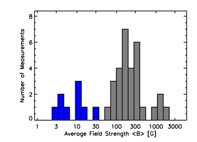
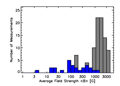
Figure 6: Magnetic field measurements from Stokes I (grey histograms) and Stokes V (blue histograms) in G- and K-type stars (left panel) and M stars (right panel).

Most direct measurements of magnetic fields were carried out either in Stokes I or Stokes V [Kochukhov et al., 2011, (but see Kochukhov et al., 2011)]. The observational systematics of the methods lead to significant biases that need to be understood if we want to interpret the results. For example, Stokes I measurements have a hard time detecting weak magnetic fields in rapid rotators, but they capture almost all field components. Stokes V measurements, on the other hand, can detect very small fields but cancellation of opposite field directions can make significant field components invisible.

A collection of Stokes I and Stokes V average magnetic field measurements is shown in Fig. 6 [Reiners, 2012, (data collection from Reiners, 2012)]. Stokes I measurements find magnetic fields of several 100 G and more, smaller fields cannot be detected because of limited sensitivity. Stokes V measurements in G- and K-type stars are limited to field strengths of a few 10 G, which is probably because of cancellation effects. In M-stars, the detected fields are significantly larger.

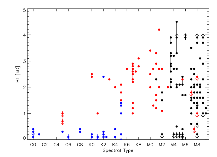
Figure 7: Observations of Stokes I average magnetic fields in different types of stars. Blue: G- and K-dwarfs; black: M-dwarfs; red: pre-MS stars.

In Fig. 7, Stokes I measurements for stars of spectral types G0–M9 are shown as a function of spectral type. Field stars are shown together with pre-main sequence stars. The magnetic fields found in late-type stars are higher than in hotter stars, but not all late-type stars have strong fields. The driver of magnetic field generation is rotation; the distribution in Fig. 7 reflects the distribution of rotation velocities in stars of different spectral type and age. Furthermore, it reflects the fact that strong fields are much more difficult to observe in G stars than in M stars. The reason is the following: A field strength of ca. 1000 G can be expected in stars with Rossby numbers $Ro\approx 0.2$. According to Fig. 4, the equatorial rotation velocity of a G2-star at this rotation rate is $v_{\mathrm{eq}}\approx 10$ km s^-1. In an M0 star with the same Rossby number, the equatorial rotation velocity is only $v_{\mathrm{eq}}\approx 3$ km s^-1, and in an M4 star we find $v_{\mathrm{eq}}\approx 1$ km s^-1. The signature of magnetic fields at low Rossby numbers is therefore much more obvious in low-mass stars.

References

- [Basri et al., 2013] Basri, G., Walkowicz, L.M. & Reiners, A., 2013, ApJ, 769, 37
- [Chabrier & Küker, 2006] Chabrier, G. & Küker, M., 2006, A&A, 446, 1027
- [Charbonneau, 2010] Charbonneau, P., 2010, Living Rev. Solar Phys., 7
- [Durney & Latour, 1978] Durney, B.R, & Latour, J., 1978, Geophys. Astrophys. Fluid Dyn., 9, 241
- [Gray, 2008] Gray, D.F., 2008, The Observation and Analysis of Stellar Photospheres, Cambridge University Press
- [Kiraga & Stepien, 2007] Kiraga, M. & Stepien, K., 2007, Acta Astron., 57, 149
- [Kochukhov et al., 2011] Kochukhov, O., Makaganiuk, V., Piskunov, N., Snik, F., Jeffers, S. V., Johns-Krull, C. M., Keller, C. U., Rodenhuis, M., & Valenti, J. A., ApJ, 732, 19
- [Noyes et al., 1984] Noyes, R.W., Hartmann, L.W., Baliunas, S.L., Duncan, D.K., & Vaughan, A.H., 1984, ApJ, 279, 763
- [Ossendrijver, 2003] Ossendrijver, M.A.J.H., 2003, AAR, 11, 287
- [Pizzolato et al., 2003] Pizzolato, N., Maggio, A., Micela, G., Sciortino, S., & Ventura, P., 2003, A&A, 397, 147
- [Reiners et al., 2009] Reiners, A., Basri, G., & Browning, M., 2009, ApJ, 692, 538
- [Reiners, 2012] Reiners, A., 2012, Living Rev. Solar Phys., 8, 1
- [Tinbergen, 1996] Tinbergen, J., 1996, Astronomical Polarimetry, Cambridge University Press
- [Wright et al., 2011] Wright, N.J, Drake, J.J., Mamajek, E.E., & Henry, G.W., 2011, ApJ, 743, 48