On the Gross-Pitaevskii equation with pumping and decay: stationary states and their stability

Abstract

We investigate the behavior of solutions of the complex Gross-Pitaevskii equation, a model that describes the dynamics of pumped decaying Bose-Einstein condensates. The stationary radially symmetric solutions of the equation are studied and their linear stability with respect to two-dimensional perturbations is analyzed. Using numerical continuation, we calculate not only the ground state of the system, but also a number of excited states. Accurate numerical integration is employed to study the general nonlinear evolution of the system from the unstable stationary solutions to the formation of stable vortex patterns.

1 Introduction

In this paper, we explore numerically the behavior of solutions of the complex Gross-Pitaevskii (GP) equation:

$$\begin{array}[]{lll}i\psi_{t}=-\Delta\psi+V\left(x\right)\psi+\left|\psi\right|^{2}\psi+i\left[\omega\left(x\right)-\sigma\left|\psi\right|^{2}\right]\psi,&t>0,&x\in D=\mathbb{R}^{2},\\ \psi\left(x,0\right)=\psi_{0}\left(x\right),\>x\in D,\end{array}$$ (1)

where $\psi=\psi\left(x,t\right)$ represents the wave function, $V\left(x\right)$ is the trapping potential, $\omega=\omega\left(x\right)\geq 0$ is the pumping term, and $\sigma>0$ is the strength of the decaying term. Equation (1) was proposed by Keeling and Berloff [25] to study pumped decaying condensates, particularly the Bose-Einstein condensates (BEC) of exciton-polaritons.

We use accurate numerical techniques to investigate the nature of the radially symmetric stationary solutions of (1), their linear stability properties, and the long-time nonlinear evolution of the solutions of (1) that start with the unstable stationary states as initial conditions. The stationary radially symmetric solutions of the complex GP equation are computed by using a numerical collocation method. Such stationary solutions are found to be linearly unstable with respect to two-dimensional perturbations when the pumping region is small as well as when it is large. Linearly stable solutions are used as a starting point in a numerical continuation method, wherein the stationary solutions are computed when a parameter in the equation is varied. A number of different stationary solutions are found at any given set of parameters. Among these solutions, the linearly stable one is seen to have the smallest chemical potential. Such solution is denoted as the ground state, while the other solutions are termed the excited states. With the stationary solutions and their linear stability properties known, we then implement a time-splitting spectral method to solve (1) and explore the nonlinear dynamics of the solutions.

The GP equation and its variants are widely used to understand BEC in various systems. The possibility of condensation of bosons was predicted by Bose [10] and Einstein [18, 19] in 1924-1925. The condensate was obtained experimentally for the first time in 1995 [2, 11, 15] in a system consisting of about half a million alkali atoms cooled down to nanokelvin-level temperatures. The principal interest in BEC lies in its nature as a macroscopic quantum system. Some of the dynamics of atomic BEC have been successfully described by the GP equation [22, 28, 29], a nonlinear Schrödinger equation,

$$i\hbar\psi_{t}=-\frac{\hbar^{2}}{2m}\triangle\psi+V\left(\mathbf{x}\right)\psi+\delta\left|\psi\right|^{2}\psi,$$ (2)

derived from the mean field theory of weakly interacting bosons. Here, $\psi=\psi(\mathbf{x},t)$ is the wave function of the condensate, $\delta$ is a constant characterizing the strength of the boson-boson interactions, $m$ is the mass of the particles, and $V(\mathbf{x})$ is the trapping potential.

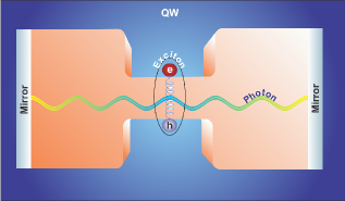
Figure 1: Schematics of the exciton-polariton microcavity.

A serious obstacle in the study of BEC in atomic systems is the extremely low temperatures required to create the condensate. Because of this difficulty, other, non-atomic systems are being explored that can undergo condensation at higher temperatures. One possible candidate is a system of exciton-polaritons, which are quasi-particles that can be created in semi-conductor cavities as a result of interaction between excitons and a laser field in the cavity [23, 13]. A two-dimensional quantum structure consisting of coupled quantum wells embedded in an optical microcavity is used (see Fig. 1). Excitons are electron-hole pairs, produced in the coupled quantum wells, that interact with the photons trapped inside the optical cavity by means of two highly reflective mirrors. Due to this confinement, the effective mass of the polaritons is very small: $10^{-4}$ times the free electron mass [23]. Since the temperature of condensation is inversely proportional to the mass of the particles, the exciton-polariton systems afford relatively high temperatures of condensation. There are, however, two drawbacks in this new condensate: the polaritons are highly unstable and exhibit strong interactions. The excitons disappear with the recombination of the electron-hole pairs through emission of photons. One way to deal with this problem is to introduce a polariton reservoir: polaritons are “cooled” and “pumped” from this reservoir into the condensate to compensate for the decay. At the same time, a low density level is kept in order to reduce the interactions between polaritons. For a detailed study of this system, see, e.g., [1, 9, 24].

Various mathematical models have been proposed for this new condensate [25, 30, 31]. One of them, called complex GP equation [25], is explored in this paper. The complex GP equation reflects the non-equilibrium dynamics described above by adding pumping and decaying terms to the GP equation. In [25], the authors observed the formation of two-dimensional vortex lattices. Linear stability of stationary solutions and the formation of dark solitons in the one-dimensional complex GP equation were analyzed by Cuevas et al. [14]. The role of damping in the absence of the pumping term in the GP equation is studied by, e.g., Bao et al. [7] and Antonelli et al. [3].

The remainder of the paper is organized as follows. In Section 2, the stationary radial solutions of the complex GP equation are calculated. In Section 3, a numerical collocation method is used to compute the solutions described in Section 2. In Section 4, the linear stability of the stationary states is analyzed. In Section 5, the numerical continuation of one of the linearly stable solutions is carried out, showing some of the excited states. In Section 6, the full complex GP equation is solved numerically by a second order time-splitting spectral method. Conclusions are drawn in Section 7.

2 Stationary radial solutions

Let us analyze solutions of (1) of the form $\psi\left(x,t\right)=\exp\left(-i\mu t\right)\phi\left(x\right)$, where $\mu$ corresponds to the real-valued chemical potential and $\phi$ represents the amplitude function that vanishes as $\left|x\right|\rightarrow\infty$. Introducing this ansatz into (1) leads to the following equation for $\phi$,

$$\mu\phi\left(x\right)=\left[-\Delta+V\left(x\right)+\left|\phi\left(x\right)\right|^{2}+i\left(\omega\left(x\right)-\sigma\left|\phi\left(x\right)\right|^{2}\right)\right]\phi\left(x\right).$$ (3)

Multiplying (3) by $\phi^{*}$ (the complex conjugate of $\phi$) and integrating over $D=\mathbb{R}^{2}$ yields

$$\mu\int_{D}\left|\phi\left(x\right)\right|^{2}dx=\int_{D}\left[\left|\nabla\phi\left(x\right)\right|^{2}+V\left(x\right)\left|\phi\left(x\right)\right|^{2}+\left|\phi\left(x\right)\right|^{4}+i\left(\omega\left(x\right)-\sigma\left|\phi\left(x\right)\right|^{2}\right)\left|\phi\left(x\right)\right|^{2}\right]dx.$$ (4)

It follows immediately that, for $\mu$ to be real, it must be required that

$$\int_{D}\left(\omega\left(x\right)-\sigma\left|\phi\left(x\right)\right|^{2}\right)\left|\phi\left(x\right)\right|^{2}dx=0.$$ (5)

Note that allowing $\mathrm{Im}(\mu)\neq 0$ would lead to exponential growth ($\mathrm{Im}\left(\mu\right)>0$) or exponential decay to zero ($\mathrm{Im}\left(\mu\right)<0$) of the solution, since in this case $\psi\left(x,t\right)=\exp\left(-i\mathrm{Re}\left(\mu\right)t\right)\exp\left(\mathrm{Im}\left(\mu\right)t\right)\phi\left(x\right)$.

An alternative approach to study the stationary solutions of (1) is given by its quantum hydrodynamic version. For this, define $S=S\left(x,t\right)$ as the phase of $\psi$ and $\rho=\rho\left(x,t\right)=\left|\psi\left(x,t\right)\right|^{2}$. Hence, inserting the ansatz $\psi=\sqrt{\rho}\exp\left(iS\right)$ into (1) and separating real and imaginary parts yields

$$\frac{1}{2}\rho_{t}+\mathrm{div}J-\left(\omega\left(x\right)-\sigma\rho\right)\rho= 0,$$ (6)

$$S_{t}+\left|\nabla S\right|^{2}+V-\frac{\triangle\sqrt{\rho}}{\sqrt{\rho}}+\rho= 0,$$ (7)

where $J=J\left(x,t\right)=\mathrm{Im}\left(\psi^{*}\nabla\psi\right)$ is the current density. Taking the gradient of (7), multiplying by $\rho$, and using (6) and $\mathrm{div}\left(J\otimes J/\rho\right)=\frac{1}{2}\rho\nabla\left|\nabla S\right|^{2}+\nabla S\cdot\mathrm{div}J$ gives the following equivalent expression of (7):

$$J_{t}+2\mathrm{div}\left(\frac{J\otimes J}{\rho}\right)+\rho\nabla V-\rho\nabla\left(\frac{\triangle\sqrt{\rho}}{\sqrt{\rho}}\right)+\frac{1}{2}\nabla\rho^{2}=2\left(\omega\left(x\right)-\sigma\rho\right)J.$$ (8)

Gasser and Markowich [20] showed that each of the terms in (8), in particular, the nonlinear terms with singularities in the vacuum state ($\rho\equiv 0$), are well defined in the sense of distributions if finite kinetic energy solutions are considered, i.e.,

$$\int_{D}\left|\nabla\psi\right|^{2}dx<\infty.$$

Using this result, the next theorem can be deduced from (6) and (8).

Theorem 1.

Let $\omega=\omega\left(x\right)\geq 0$ be smooth with $\left\{\left.x\right|\omega\left(x\right)>0\right\}$ simply connected. Then there exists a stationary solution of (6)-(8) with $J\equiv 0$ if and only if either

1. $\rho\equiv 0$, or

2. $\rho=\frac{\omega\left(x\right)}{\sigma}$. In this case, $V(x)=C+\frac{\triangle\sqrt{\omega\left(x\right)}}{\sqrt{\omega\left(x\right)}}-\frac{1}{\sigma}\omega\left(x\right)$ in $\left\{\left.x\right|\omega\left(x\right)>0\right\}$, where $C$ is a constant.

Proof.

Set $\rho_{t}\equiv 0$, $J_{t}\equiv 0$, and $J\equiv 0$ in (6) and (8). Then, statement 1 is a trivial solution of the system. For statement 2, notice that (6) yields $\rho=\omega\left(x\right)/\sigma$. Inserting this expression into (8) gives

$$\begin{array}[]{cc}\nabla\left(V\left(x\right)-\frac{\triangle\sqrt{\omega\left(x\right)}}{\sqrt{\omega\left(x\right)}}+\frac{1}{\sigma}\omega\right)=0,&\mathrm{in\>}\left\{\left.x\right|\omega\left(x\right)>0\right\}\end{array}.$$

Hence,

$$\begin{array}[]{cc}V\left(x\right)=C+\frac{\triangle\sqrt{\omega\left(x\right)}}{\sqrt{\omega\left(x\right)}}-\frac{1}{\sigma}\omega,&\mathrm{in\>}\left\{\left.x\right|\omega\left(x\right)>0\right\},\end{array}$$ (9)

where $C$ is a constant.

Now, if statement 1 is true, then $J\equiv 0$ follows immediately. On the other hand, if statement 2 is valid, then (7) gives $\left|\nabla S\right|^{2}=0$, which implies $\nabla S=0$. Thus, $J\left(=\rho\nabla S\right)\equiv 0$ .∎

Remark 2.

The stationary GP equation,

$$\begin{array}[]{cc}V(x)=\mu+\frac{\triangle\phi}{\phi}-\frac{1}{\sigma}\left|\phi\right|^{2},&\phi\neq 0,\end{array}$$ (10)

has exactly the form of (9), with $C=\mu$ (the chemical potential). Then, letting $\omega\left(x\right)=\left|\phi\right|^{2}$ (the density profile of any solution of (10)), the solution of the corresponding complex GP equation is given by $\rho=\left|\phi\right|^{2}/\sigma$ with $J\equiv 0$.

Now, going back to (6), and integrating in space gives

$$\frac{1}{2}\frac{dM}{dt}=\int_{D}\left(\omega\left(x\right)-\sigma\rho\right)\rho dx,$$

where

$$M\equiv\int_{D}\rho dx$$

is the $mass$ of the system. Therefore, we can see that equation (3) along with condition (5) lead to solutions where the pumping and decaying parts equilibrate, i.e., the time derivative of the mass of the system is zero. In addition, condition (5) ensures that the chemical potential is a nonnegative real quantity.

For the rest of the paper, $V(x)=\left|x\right|^{2}$ is the harmonic potential and $\omega\left(x\right)=\alpha\Theta\left(R-\left|x\right|\right)$, where $\alpha>0$ is the strength of the pumping term and $R>0$ is the radius of the pumping region delimited by the smoothed Heaviside function $\Theta\left(x\right)=\left(1+\tanh\left(\kappa x\right)\right)/2$ for some fixed parameter $\kappa>0$.

In the following we investigate the stationary radially symmetric solutions of (3). In this case, (3) becomes $(\begin{array}[]{cc}{}^{\prime}=\frac{d}{dr},&\Theta_{R}=\Theta\left(R-r\right)\end{array})$

$$\mu\phi=-\phi^{\prime\prime}-\frac{1}{r}\phi^{\prime}+r^{2}\phi+\left|\phi\right|^{2}\phi+i\left(\alpha\Theta_{R}-\sigma\left|\phi\right|^{2}\right)\phi,$$ (11)

where $r=\left|x\right|\geq 0$, with the boundary conditions $\phi\left(r\right)=0$ as $r\rightarrow\infty$ and $\phi^{\prime}\left(0\right)=0$. Condition (5) is written as

$$\intop_{0}^{\infty}\left(\alpha\Theta_{R}-\sigma\left|\phi\left(r\right)\right|^{2}\right)\left|\phi\left(r\right)\right|^{2}rdr=0.$$ (12)

By defining

$$\xi\left(r\right)=\int_{0}^{r}\left(\alpha\Theta_{R}-\sigma\left|\phi\left(s\right)\right|^{2}\right)\left|\phi\left(s\right)\right|^{2}sds,$$ (13)

condition (12) can be expressed as

$$\xi^{\prime}\left(r\right)=\left(\alpha\Theta_{R}-\sigma\left|\phi\left(r\right)\right|^{2}\right)\left|\phi\left(r\right)\right|^{2}r,$$ (14)

with

$$\xi\left(\infty\right)=0.$$ (15)

The variable $\xi$ is convenient for subsequent numerical integration. The constancy of the chemical potential $\mu$ can be written as

$$\mu^{\prime}\left(r\right)=0.$$ (16)

Because the phase of $\phi$ is arbitrary, we let

$$\mathrm{Im}\left(\phi\left(0\right)\right)=0.$$ (17)

Notice that the second order ordinary differential equation (ODE) (11) can be expanded as a system of two first-order ODE. Due to the harmonic trapping potential and the finite pumping region, the solution is expected to be concentrated on a bounded domain. This fact is used in the numerical computations, where the integration domain is chosen as $D=\left[0,b\right]$ for large enough $b$. Then, the right boundary conditions, $\phi\left(\infty\right)=0$ and $\xi\left(\infty\right)=0$, are replaced by $\phi\left(b\right)=0$ and $\xi\left(b\right)=0$, respectively. As a result, the following set of ODE is obtained for $r\in\left[0,b\right]$:

$$\begin{array}[]{ccl}\phi^{\prime}&=&\varphi,\\ \varphi^{\prime}&=&-\frac{1}{r}\varphi-\mu\phi+r^{2}\phi+\left|\phi\right|^{2}\phi+i\left(\alpha\Theta_{R}-\sigma\left|\phi\right|^{2}\right)\phi,\\ \xi^{\prime}&=&\left(\alpha\Theta_{R}-\sigma\left|\phi\left(r\right)\right|^{2}\right)\left|\phi\left(r\right)\right|^{2}r,\\ \mu^{\prime}&=&0,\end{array}$$ (18)

with

$$\begin{array}[]{cccc}\phi\left(b\right)=0,&\varphi\left(0\right)=0,&\mathrm{Im}\left(\phi\left(0\right)\right)=0,&\xi\left(b\right)=0.\end{array}$$

This nonlinear boundary value problem with a singularity of the first kind (see, e.g., [16]) is consistent with respect to the number of boundary conditions. The value of $\varphi^{\prime}$ at $r=0$ can be determined using

$$\underset{r\rightarrow 0}{\lim}\frac{\varphi\left(r\right)-\varphi\left(0\right)}{r-0}=\underset{r\rightarrow 0}{\lim}\frac{\varphi\left(r\right)}{r}=\varphi_{r}\left(0\right),$$ (19)

due to the boundary condition $\varphi\left(0\right)=0$. Then, the second equation in (18) gives

$$\varphi^{\prime}\left(0\right)=\frac{1}{2}\left[-\mu\phi\left(0\right)+\left|\phi\left(0\right)\right|^{2}\phi\left(0\right)+i\left(\alpha-\sigma\left|\phi\left(0\right)\right|^{2}\right)\phi\left(0\right)\right].$$ (20)

It is convenient to make (18) real valued, autonomous, and restricted to the interval $\left[0,1\right]$. Substituting $\phi=\theta+i\eta$ into (11), separating real and imaginary parts, and writing the resulting equations as a system of first order ODE, leads to a real valued system. In order to make (18) autonomous, define $\varrho(r)=r$ such that $\varrho^{\prime}(r)=1$ and $\varrho\left(0\right)=0$ are added to the system. Finally, rescaling $r$ as $\tilde{r}=\frac{r}{b}$, restricts the domain to the interval $[0,1]$. Thus, (18) becomes (${}^{\prime}=\frac{d}{d\tilde{r}}$):

$$\begin{array}[]{ccl}\frac{1}{b}\theta^{\prime}&=&\varphi,\\ \frac{1}{b}\varphi^{\prime}&=&-\frac{1}{\varrho}\varphi-\mu\theta+\varrho^{2}\theta+\left(\theta^{2}+\eta^{2}\right)\theta-\left(\alpha\Theta\left(R-\varrho\right)-\sigma\left(\theta^{2}+\eta^{2}\right)\right)\eta,\\ \frac{1}{b}\eta^{\prime}&=&\zeta,\\ \frac{1}{b}\zeta^{\prime}&=&-\frac{1}{\varrho}\zeta-\mu\eta+\varrho^{2}\eta+\left(\theta^{2}+\eta^{2}\right)\eta+\left(\alpha\Theta\left(R-\varrho\right)-\sigma\left(\theta^{2}+\eta^{2}\right)\right)\theta,\\ \frac{1}{b}\xi^{\prime}&=&\left(\alpha\Theta\left(R-\varrho\right)-\sigma\left(\theta^{2}+\eta^{2}\right)\right)\left(\theta^{2}+\eta^{2}\right)\varrho,\\ \frac{1}{b}\mu^{\prime}&=&0,\\ \frac{1}{b}\varrho^{\prime}&=&1,\end{array}$$ (21)

with

$$\begin{array}[]{ccccccc}\varphi\left(0\right)=0,&\theta\left(1\right)=0,&\zeta\left(0\right)=0,&\eta\left(0\right)=0,&\eta\left(1\right)=0,&\xi\left(1\right)=0,&\varrho\left(0\right)=0.\end{array}$$

3 Collocation method

System (21) can be solved with high accuracy by using a collocation method. The basic idea involves forming an approximate solution as a linear combination of a set of functions (usually polynomials), the coefficients of which are determined by requiring the combination to satisfy the system at certain points (the collocation points) as well as the boundary conditions.

To introduce the algorithm, consider the following first-order system of ODE:

$$\begin{array}[]{ccc}u^{\prime}\left(r\right)=f\left(u\left(r\right)\right),&r\in I=\left[0,1\right],&u\left(\cdot\right),f\left(\cdot\right)\in\mathbb{R}^{d}\end{array},$$ (22)

subject to the boundary conditions

$$\begin{array}[]{cc}b\left(u\left(0\right),u\left(1\right)\right)=0,&b\left(\cdot\right)\in\mathbb{R}^{d}.\end{array}$$

Let $I_{h}=\left\{r_{n}:0=r_{0}<r_{1}<\cdots<r_{N}=1\right\}$ be a given mesh on $I$, with $h_{n}=r_{n}-r_{n-1}$ $\left(n=1,\ldots,N\right)$. Define the space of vector-valued piecewise polynomials, $\mathcal{P}^{m}\left(I_{h}\right)$, as

$$\mathcal{P}^{m}\left(I_{h}\right)=\left\{v\in C\left(I\right):\begin{array}[]{cc}v\mid_{\left[r_{n-1},r_{n}\right]}\in\pi_{m},&\left(1\leq n\leq N\right)\end{array}\right\},$$

where $\pi_{m}$ is the space of all vector-valued polynomials of degree $\leq m$. The collocation method consists of finding an element $q_{h}\in\mathcal{P}^{m}\left(I_{h}\right)$ that approximates the solution of (22). Such approximation will be found by requiring $q_{h}$ to satisfy (22) on a given finite subset, $S_{h}$, of $I$, as well as the boundary conditions.

Let $S_{h}$, the set of collocation points, be given by

$$S_{h}=\left\{r_{n,i}=r_{n-1}+c_{i}h_{n}:\begin{array}[]{cc}1\leq n\leq N,&0=c_{1}<c_{2}<\cdots<c_{m}=1\end{array}\right\},$$

where $\left\{c_{i}\right\}$ are usually Gauss, Radau, or Lobatto points (see, e.g., Ascher et al. [4]). The collocation solution $q_{h}\in\mathcal{P}^{m}\left(I_{h}\right)$ for (22) is defined by the equation

$$\begin{array}[]{ccc}q^{\prime}_{h}\left(r_{n,i}\right)=f\left(q_{h}\left(r_{n,i}\right)\right),&r_{n,i}\in S_{h},&b\left(q_{h}\left(0\right),q_{h}\left(1\right)\right)=0.\end{array}$$

Now, consider a local Lagrange basis representation of $q_{h}$. Define

$$\begin{array}[]{ccc}L_{i}\left(\delta\right):=\overset{m}{\underset{k=1,k\neq i}{\prod}}\frac{\delta-c_{k}}{c_{i}-c_{k}},&\left(i=1,...,m\right),&\delta\in\left[0,1\right].\end{array}$$

Then the local polynomials can be written as

$$q_{n}\left(r_{n-1}+\delta h_{n}\right)=\sum_{i=1}^{m}L_{i}\left(\delta\right)q_{h}\left(r_{n-1}+c_{i}h_{n}\right),\begin{array}[]{cc}1\leq n\leq N,&\delta\in\left[0,1\right].\end{array}$$

The collocation equations are, therefore,

$$\begin{array}[]{ccc}q^{\prime}_{n}\left(r_{n,i}\right)=f\left(q_{n}\left(r_{n,i}\right)\right),&r_{n,i}\in S_{h},&1\leq n\leq N,\end{array}$$ (23)

with the boundary conditions

$$\begin{array}[]{cc}b_{l}\left(u_{0},u_{N}\right)=0,&l=1,...,d.\end{array}$$ (24)

Equations (23) - (24) can be solved by a Newton-Chord iteration. It can be proven that if the solution $u\left(r\right)$ of the boundary value problem is sufficiently smooth, then the order of accuracy of the method is $m$, i.e., $\left\|q_{h}-u\right\|_{\infty}=\mathcal{O}\left(h^{m}\right)$, where $h:=\max\left\{h_{n}:1\leq n\leq N\right\}$ (the diameter of the mesh $I_{h}$). For a detailed description of this method, the reader is referred to Ascher et al. [4] and Brunner [12].

The Matlab function $\mathit{bvp5c}$ is used to solve system (21) by the collocation method. This function implements a four-point Lobatto method capable of handling singularities of the first kind and mesh adaptation. In addition, $\mathit{bvp5c}$ can converge even if the initial guess is not very close to the solution; that is, the function converges by using as an initial guess the Thomas-Fermi profile [25]:

$$\left|\phi\right|^{2}=\begin{cases}\begin{array}[]{cc}\tilde{\mu}-r^{2},&r<\sqrt{\tilde{\mu}},\\ 0,&r\geq\sqrt{\tilde{\mu}},\end{array}&\tilde{\mu}=3\alpha/2\sigma.\end{cases}$$ (25)

It is important to note that $\mathit{bvp5c}$ always evaluates the ODE at the end points. Then, due to the singularity, the value obtained in (20) must be supplied to $\mathit{bvp5c}$ when evaluating the ODE at $r=0$.

With 6000 grid points (initially equispaced) on the domain $D=[0,15]$, the maximum residual obtained is less than $10^{-11}$ for the different cases studied: $\alpha=4.4$, $\sigma=0.3$, $\kappa=10$, and $0<R<10$. In the following section, a linear stability analysis is performed on these results, which are later used as a starting point in the numerical continuation.

4 Linear stability analysis of the radially symmetric solutions

Consider the radially symmetric solutions $\psi\left(r,t\right)=\exp\left(-i\mu t\right)\phi\left(r\right)$ obtained in the previous section. To study their linear stability, small perturbations of the wave function can be expressed as

$$\psi\left(r,\theta,t\right)=\exp\left(-i\mu t\right)\left[\phi\left(r\right)+\varepsilon\left(u\left(r\right)\exp\left(-i\left(m\theta+\omega t\right)\right)+v^{*}\left(r\right)\exp\left(i\left(m\theta+\omega^{*}t\right)\right)\right)\right],$$ (26)

with $\varepsilon<<1$, $m=1,2,3,...$

This form of the perturbation and the subsequent calculations are known as Bogoliubov-De Gennes analysis. Notice that the perturbation is time dependent with frequency $\omega$ and complex amplitude functions $u\left(r\right)$ and $v\left(r\right)$. In addition, the perturbation is both radial and angular, where the angular part is tested with different modes given by $m$. The radially symmetric solutions are linearly unstable if $\mathrm{Im}\left(\omega\right)>0$.

We proceed by evaluating the complex GP equation for the trial wave function (26) to $\mathcal{O}\left(\varepsilon\right)$. To simplify the notation, we write $\phi\left(r\right)$, $u\left(r\right)$ and $v\left(r\right)$ as $\phi$, $u$ and $v$, respectively. Equating terms in $\exp\left(-i\mu t\right)$ yields the equation for the radially symmetric solutions:

$$\mu\phi=\left(-\frac{d^{2}}{dr^{2}}-\frac{1}{r}\frac{d}{dr}+r^{2}+\left|\phi\right|^{2}+i\left(\alpha\Theta_{R}-\sigma\left|\phi\right|^{2}\right)\right)\phi.$$ (27)

Equating terms in $\exp\left(-i\left(m\theta+\left(\mu+\omega\right)t\right)\right)$ leads to

$$\begin{array}[]{ccc}\left(\mu+\omega\right)u&=&\left(-\frac{d^{2}}{dr^{2}}-\frac{1}{r}\frac{d}{dr}+\frac{m^{2}}{r^{2}}+r^{2}+2\left|\phi\right|^{2}+i\left(\alpha\Theta_{R}-2\sigma\left|\phi\right|^{2}\right)\right)u+\left(1-i\sigma\right)\phi^{2}v.\end{array}$$ (28)

Equating terms in $\exp\left(i\left(m\theta-\left(\mu-\omega^{*}\right)t\right)\right)$ gives

$$\begin{array}[]{ccc}\left(\mu-\omega^{*}\right)v^{*}&=&\left(-\frac{d^{2}}{dr^{2}}-\frac{1}{r}\frac{d}{dr}+\frac{m^{2}}{r^{2}}+r^{2}+2\left|\phi\right|^{2}+i\left(\alpha\Theta_{R}-2\sigma\left|\phi\right|^{2}\right)\right)v^{*}+\left(1-i\sigma\right)\phi^{2}u^{*}.\end{array}$$ (29)

Taking the complex conjugate of (29) produces

$$\begin{array}[]{ccc}\left(\mu-\omega\right)v&=&\left(-\frac{d^{2}}{dr^{2}}-\frac{1}{r}\frac{d}{dr}+\frac{m^{2}}{r^{2}}+r^{2}+2\left|\phi\right|^{2}-i\left(\alpha\Theta_{R}-2\sigma\left|\phi\right|^{2}\right)\right)v+\left(1+i\sigma\right)\left(\phi^{*}\right)^{2}u.\end{array}$$ (30)

Finally, equations (28) and (30) can be written as

$$\left[\begin{array}[]{rr}L_{1}&L_{2}\\ -L_{2}^{*}&-L_{1}^{*}\end{array}\right]\left[\begin{array}[]{c}u\\ v\end{array}\right]=\omega\left[\begin{array}[]{c}u\\ v\end{array}\right],$$ (31)

with

$$\begin{array}[]{ccl}L_{1}&=&-\mu-\frac{d^{2}}{dr^{2}}-\frac{1}{r}\frac{d}{dr}+\frac{m^{2}}{r^{2}}+r^{2}+2\left|\phi\right|^{2}+i\left(\alpha\Theta_{R}-2\sigma\left|\phi\right|^{2}\right)\\ &=&-\mu-\frac{d^{2}}{dr^{2}}-\frac{1}{r}\frac{d}{dr}+\frac{m^{2}}{r^{2}}+r^{2}+2\left(1-i\sigma\right)\left|\phi\right|^{2}+i\alpha\Theta_{R},\end{array}$$

and

$$L_{2}=\left(1-i\sigma\right)\phi^{2}.$$

The eigenvalue problem (31) is discretized by using centered differences and solved with the Matlab function $eig$. The results for $R=2$ are plotted in Fig. (2). Figure (2.b) shows the maximum imaginary part of the eigenvalues, $\omega$, for $m=1,2,...,50$. Notice that all of them are negative; thus, the solution is linearly stable under these perturbations. Taking this into account, this solution will be used as a starting point in the numerical continuation method presented in the following section.

Figures (3) and (4) show two cases where the solutions are linearly unstable. An interesting observation is the fact that the radially symmetric solutions are the same for large enough values of $R$; we note that this is the case for $R=8$ and $R=9$. This characteristic was also observed by Cuevas et al. [14] for the one-dimensional complex GP equation.

Fig (5) shows the maximum imaginary part of the eigenvalues, $\omega$, for $0<R<10$, with spacing of 0.1 in $R$ and for $m=1,2,...,50$. Notice that for large values of $R$, which in this case also implies large mass, the solutions become unstable. However, the solutions are also unstable for small values of $R$ (small mass), i.e. at $R\lesssim 0.6$. For $R\lesssim 0.6$ it was observed that a different branch of solutions with smaller chemical potential, $\mu$, becomes stable. The case of large values of $R$ is studied in detail in Section 6.

Finally, Fig (6) shows the magnitude of the current, $\left|J\right|$, corresponding to the solutions for $R=2,8,9$.

a)

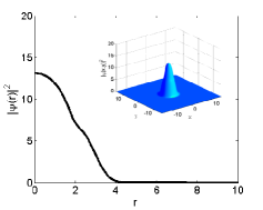
b)

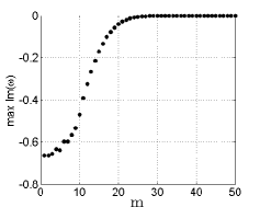
Figure 2: a) Density profile of the radially symmetric solution for $R=2$, with the two-dimensional view shown in the inset. b) Result from the linear stability analysis: the plot shows the maximum imaginary part of the eigenvalues, $\omega$, for $m=1,2,...,50$.

a)

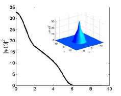
b)

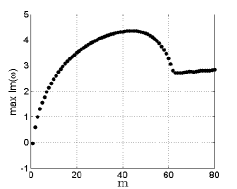
Figure 3: a) Density profile of the radially symmetric solution for $R=8$, with the two-dimensional view shown in the inset. b) Result from the linear stability analysis: the plot shows the maximum imaginary part of the eigenvalues, $\omega$, for $m=1,2,...,50$.

a)

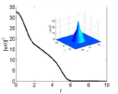
b)

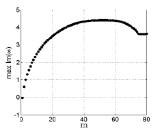
Figure 4: a) Density profile of the radially symmetric solution for $R=9$, with the two-dimensional view shown in the inset. b) Result from the linear stability analysis: the plot shows the maximum imaginary part of the eigenvalues, $\omega$, for $m=1,2,...,50$.

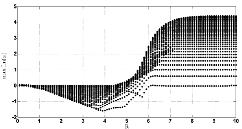
Figure 5: Results for $0<R<10$ (with spacing of 0.1) showing the maximum imaginary part of the eigenvalues $\omega$ for $m=1,2,...,50$. Instability exists at both $R\lesssim 0.6$ and $R\gtrsim 4.4$.

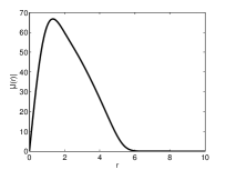
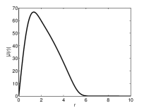
Figure 6: Magnitude of the current $J$ corresponding to the solutions for $R=2$ (left), $R=8$ (center), and $R=9$ (right).

5 Numerical continuation for the stationary solutions

Let us rewrite system (21) as

$$F\left(u,\lambda\right)=0,$$ (32)

where $u$ is the solution of the system ($u\in\mathcal{B}$, a real Banach space), $\lambda$ is a real parameter ($\lambda$ can be $\alpha$, $\sigma$, or $R$), and $F$ is a continuously differentiable operator such that $F:\mathcal{B}\times\mathbb{R}\rightarrow\mathcal{B}$. The idea in this section is to study the dependence of the solution, $u\left(\lambda\right)$, on the parameter, $\lambda$, i.e., to trace the solution branches $\left[u\left(\lambda\right),\lambda\right]$ of (32). Since the operator, $F$, is nonlinear in $u$ and $\lambda$, this can be performed numerically by Newton’s method: suppose that $\left(u_{0},\lambda_{0}\right)$ is a solution of the discretized problem (32) and that the directional derivative $\dot{u}_{0}=du_{0}/d\lambda$ is known. Then, the solution $u_{1}$ at $\lambda_{1}=\lambda_{0}+\Delta\lambda$ (where $\Delta$ represents a small increment) can be computed as

$$\begin{cases}\begin{array}[]{c}F_{u}\left(u_{1}^{i},\lambda_{1}\right)\Delta u_{1}^{i}=-F\left(u_{1}^{i},\lambda_{1}\right),\\ u_{1}^{i+1}=u_{1}^{i}+\Delta u_{1}^{i},\>i=0,1,2,...\end{array}\end{cases}$$

with

$$u_{1}^{0}=u_{0}+\Delta\lambda\dot{u}_{0},$$

where $F_{u}\left(u,\lambda\right)$ is the Jacobian matrix.

This method, however, is unable to handle the continuation near singular points known as turning points or folds, where the solution branch bends back on itself and $F_{u}\left(u,\lambda\right)$ becomes singular. These points are particularly important to study the excited states of the complex GP equation.

A pseudo-arclength continuation method can be used to overcome this problem. The main difference from the previous algorithm is the parametrization of the solution in terms of a new quantity, $\nu$, that approximates the arclength, $s$, in the tangent space of the curve (instead of the parametrization by $\lambda$). This is usually accomplished by appending an auxiliary equation to (32) that approximates the arclength condition

$$\left\|\dot{u}\left(s\right)\right\|^{2}+\left|\dot{\lambda}\left(s\right)\right|^{2}=1.$$ (33)

This leads to the augmented system

$$\begin{cases}\begin{array}[]{c}F\left(u\left(\nu\right),\lambda\left(\nu\right)\right)=0,\\ N\left(u\left(\nu\right),\lambda\left(\nu\right),\nu\right)=0,\end{array}\end{cases}$$ (34)

with unknowns $u\left(\nu\right)$ and $\lambda\left(\nu\right)$. Then, Newton’s method (or one of its variants) can be used to solve (34), in which case the Jacobian of the system becomes the bordered matrix:

$$G=\left[\begin{array}[]{cc}F_{u}&F_{\lambda}\\ N_{u}&N_{\lambda}\end{array}\right].$$

For a detailed description of bordered matrices, see, e.g., Govaerts [21]. The function $N$ is defined such that the Jacobian $G$ is nonsingular on the solution branch, including turning points and their neighborhoods. $N\left(u,\lambda,\nu\right)\equiv\dot{u}_{0}^{T}\left(u-u_{0}\right)+\dot{\lambda}_{0}\left(\lambda-\lambda_{0}\right)-\nu$ is one of the most frequently used definitions of $N$. It was introduced by Keller [26]. With this particular definition of $N$, the method is known as Keller’s algorithm.

The pseudo-arclength continuation method can be summarized as follows: the unit tangent $\left(\dot{u}_{0},\dot{\lambda}_{0}\right)$ at $\left(u_{0},\lambda_{0}\right)$ is obtained from its definition:

$$\begin{cases}\begin{array}[]{c}F_{u}\left(u_{0},\lambda_{0}\right)\dot{u}_{0}+F_{\lambda}\left(u_{0},\lambda_{0}\right)\dot{\lambda}_{0}=0,\\ \left\|\dot{u}_{0}\right\|^{2}+\left|\dot{\lambda}_{0}\right|^{2}=1.\end{array}\end{cases}$$

Then, an approximate solution $\left(u_{a},\lambda_{a}\right)$ is computed as

$$\begin{array}[]{c}u_{a}=u_{0}+\nu\dot{u}_{0},\\ \lambda_{a}=\lambda_{0}+\nu\dot{\lambda}_{0},\end{array}$$

which is used as an initial guess in a Newton-like method for solving (34) to obtain ($u\left(\nu\right),\lambda\left(\nu\right)$).

The software package AUTO was used for the continuation of the two-dimensional radially symmetric solutions of the complex GP equation. AUTO implements Keller’s pseudo-arclength continuation algorithm. A detailed description of this algorithm can be found in Keller [27]. In addition to detecting turning points, AUTO can also find branch points, a feature that will be used to study the excited states of the complex GP equation. For the documentation of AUTO, see Doedel et al. [17].

AUTO discretizes system (21) using polynomial collocation with Gaussian points. The number of free parameters, $p$, controlled by AUTO during the continuation process is given by $p=n_{bc}+1-n$, where $n_{bc}$ is the number of boundary conditions and $n$ is the dimension of the system. Hence, the continuation for system (21) can be done in one parameter. For the results presented in this section, the number of mesh intervals is 6000, the number of Gaussian collocation points per mesh interval is 7, and the maximum absolute value of the pseudo-arclength stepsize is 0.0001. The parallel version of AUTO was run on a Beowulf-class heterogeneous computer cluster using 16 nodes for a total of 128 cores (Intel Xeon X5570, 2.93GHz).

Figure (7) shows the chemical potential, $\mu$, of the different solutions obtained by the continuation in $\sigma$ with $\alpha=4.4$ and $R=2$ fixed. By using different initial guesses (multi-bump profiles) in the collocation method described in Section 3, it was possible to find some of the solutions shown in Figs. (8) and (9). These solutions, along with the capability of AUTO to detect branch points and turning points, were employed to produce the result displayed in Fig. (7). In this figure, the red dashed line indicates the solutions corresponding to $\sigma=0.3$, $\alpha=4.4$ and $R=2$. Figs. (8) and (9) show the density profiles of these solutions. Notice that the linearly stable solution studied in Section 4 has the smallest chemical potential. In this context, this solution can be considered as the ground state solution, whereas the other solutions are excited states. In any case, an appropriate definition of the energy for this equation is necessary to determine a ground state solution. From the numerical results obtained up to now, we expect that the solution labeled 0 in Figs. (7) and (8) is the minimizer of such energy.

Equation (4) can also be used for the computation of the chemical potential. In this case

$$\mu\int_{0}^{b}\left|\phi\left(r\right)\right|^{2}rdr=\int_{0}^{b}\left[\left|\phi^{\prime}\left(r\right)\right|^{2}+r^{2}\left|\phi\left(r\right)\right|^{2}+\left|\phi\left(r\right)\right|^{4}\right]rdr,$$ (35)

where the integration domain is $\left[0,b\right]$. Using Simpson’s rule, this expression was used for a second validation of the results presented in Fig. (7).

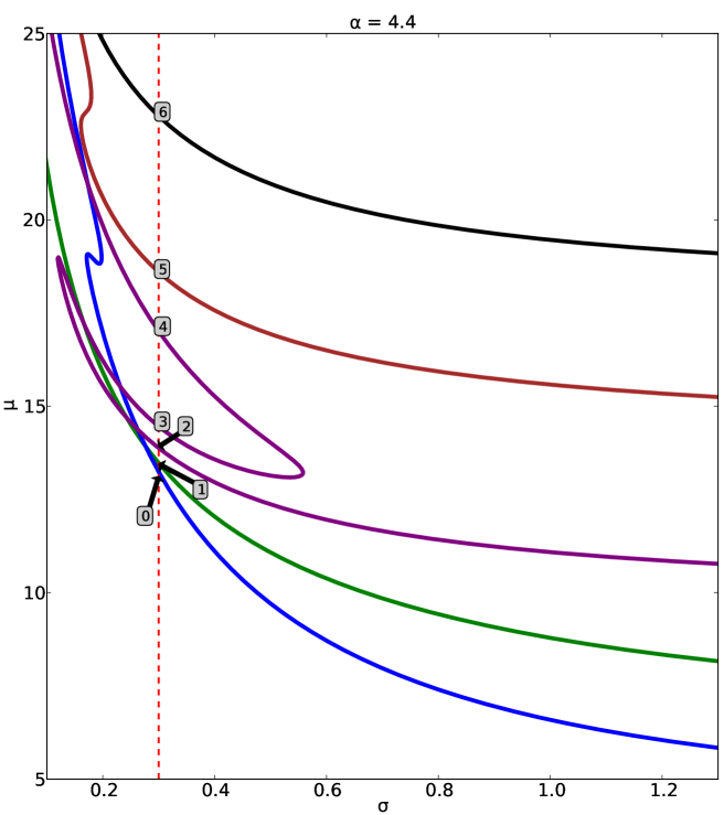
Figure 7: Result from the continuation method showing the chemical potential of the system for different values of $\sigma$ with $\alpha=4.4$ and $R=2$ fixed. The red dashed line indicates the solutions for $\sigma=0.3$. Figs. (8) and (9) show the density profiles corresponding to these solutions.

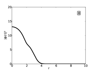
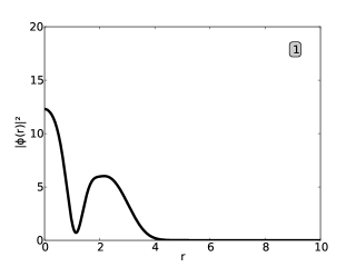
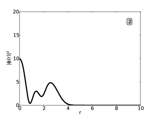
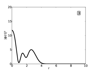
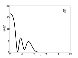
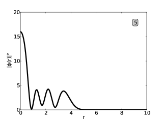
Figure 8: Density profiles of the solutions labeled 0 to 5 in Fig. (7) .

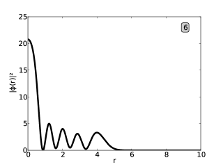
Figure 9: Density profile of the solution labeled 6 in Fig. (7)

6 Numerical integration of the complex GP equation

In this section, the numerical integration of the complex GP equation is carried out by using a Strang-splitting Fourier spectral method. This method was studied by Bao et al. [5] for the Schrödinger equation in the semiclassical regime and by Bao et al. [6] for the GP equation. For simplicity of notation, the method is presented in one dimension. The generalization to higher dimensions is straightforward using the tensor product grids. The problem can be stated as

$$\begin{array}[]{c}i\psi_{t}=-\psi_{xx}+V(x)\psi+\left|\psi\right|^{2}\psi+i\left(\alpha\Theta_{R}-\sigma\left|\psi\right|^{2}\right)\psi,\\ \psi(x,0)=\psi_{0}\left(x\right),\quad a\leq x\leq b,\quad\psi(a,t)=\psi(b,t),\quad\psi_{x}(a,t)=\psi_{x}(b,t),\quad t>0.\end{array}$$ (36)

Notice that in this case, periodic boundary conditions are specified, which are necessary for the implementation, because the discrete Fourier transform is used in one of the steps. In addition, $\psi$ is concentrated due to the trapping potential and vanishes very quickly as $\left|x\right|$ increases, making these boundary conditions a good option provided that the domain of integration is large enough.

Consider $h=\Delta x>0$ as the mesh size, with $h=(b-a)/M$, where $M$ is an even positive integer. Define $\tau=\Delta t>0$ as the time step. Let the grid points be $x_{j}=a+jh,\>j=0,1,...,M$, and the time $t_{n}=n\tau,\>n=0,1,2,...$ Finally, define $\Psi_{j}^{n}$ as the numerical approximation of $\psi(x_{j},t_{n})$. Equation (36) is now separated into

$$i\psi_{t}=V(x)\psi+\left|\psi\right|^{2}\psi+i\left(\alpha\Theta_{R}-\sigma\left|\psi\right|^{2}\right)\psi$$ (37)

and

$$i\psi_{t}=-\psi_{xx},$$ (38)

which are combined via Strang-splitting to approximate the solution of (36) on $\left[t_{n},t_{n+1}\right]$.

Step 1 of the Strang-splitting method requires the solution of (37) on a half time step, from $t_{n}$ to $t_{n}+\tau/2$. Due to the smooth Heaviside $\Theta$ in (37), two equations are solved: for $\Theta_{R}>0$

$$i\psi_{t}=V(x)\psi+\left|\psi\right|^{2}\psi+i\left(\alpha\Theta_{R}-\sigma\left|\psi\right|^{2}\right)\psi,$$ (39)

and for $\Theta_{R}=0$

$$i\psi_{t}=V(x)\psi+\left|\psi\right|^{2}\psi-i\sigma\left|\psi\right|^{2}\psi.$$ (40)

Substituting $\psi\left(x,t\right)=\rho\left(x,t\right)e^{i\theta\left(x,t\right)}$ in (39), where $\rho$ is the magnitude and $\theta$ is the phase of $\psi$, gives

$$i\rho_{t}-\rho\theta_{t}=V(x)\rho+\rho^{3}+i\left(\alpha\Theta_{R}-\sigma\rho^{2}\right)\rho.$$ (41)

Separating real and imaginary parts from (41) and looking for non-trivial solutions lead to

$$\theta_{t}=-V(x)-\rho^{2},$$ (42)

$$\rho_{t}=\left(\alpha\Theta_{R}-\sigma\rho^{2}\right)\rho.$$ (43)

The solution of (43) is given by

$$\rho=\sqrt{\frac{\rho_{0}^{2}e^{2\alpha\Theta_{R}t}}{1+\frac{\sigma}{\alpha}\rho_{0}^{2}\left(e^{2\alpha\Theta_{R}t}-1\right)/\Theta_{R}}},$$

where $\rho_{0}=\rho\left(x,0\right)$ . With this result, (42) can be solved, obtaining

$$\theta=-V(x)t-\frac{1}{2\sigma}\mathrm{ln}\left|1+\frac{\sigma}{\alpha}\rho_{0}^{2}\left(e^{2\alpha\Theta_{R}t}-1\right)/\Theta_{R}\right|+\theta_{0},$$

where $\theta_{0}$ is the phase of the initial condition.

Following the same procedure for (40) yields

$$\rho=\frac{\rho_{0}}{\sqrt{2\sigma\rho_{0}^{2}t+1}},$$

$$\theta=-V(x)t-\frac{1}{2\sigma}\mathrm{ln}\left|2\sigma\rho_{0}^{2}t+1\right|+\theta_{0}.$$

Hence, defining $\Theta_{j}\equiv\Theta\left(R-\left|x_{j}\right|\right)$, the solution of Step 1 can be written as:

$$\Psi_{j}^{(1)}=\left\{\begin{array}[]{cc}\Psi_{j}^{n}U_{j}^{(1)}e^{i\theta_{j}^{(1)}},&\Theta_{j}>0,\\ \Psi_{j}^{n}W_{j}^{(1)}e^{i\phi_{j}^{(1)}},&\Theta_{j}=0,\end{array}\right.$$

where

$$U_{j}^{(1)}=\sqrt{\frac{e^{\alpha\Theta_{j}\tau}}{1+\frac{\sigma}{\alpha}\left|\Psi_{j}^{n}\right|^{2}\left(e^{\alpha\Theta_{j}\tau}-1\right)/\Theta_{j}}},$$

$$\theta_{j}^{(1)}=-V(x_{j})\tau/2-\frac{1}{2\sigma}\mathrm{ln}\left|1+\frac{\sigma}{\alpha}\left|\Psi_{j}^{n}\right|^{2}\left(e^{\alpha\Theta_{j}\tau}-1\right)/\Theta_{j}\right|,$$

$$W_{j}^{\left(1\right)}=\frac{1}{\sqrt{\sigma\left|\Psi_{j}^{n}\right|^{2}\tau+1}},$$

$$\phi_{j}^{(1)}=-V(x_{j})\tau/2-\frac{1}{2\sigma}\mathrm{ln}\left|\sigma\left|\Psi_{j}^{n}\right|^{2}\tau+1\right|.$$

For Step 2, equation (38) has to be solved on a complete time step, from $t_{n}$ to $t_{n}+\tau$, using the solution of Step 1 as the initial condition. Equation (38) is discretized in space by the Fourier spectral method and integrated in time exactly, giving

$$\Psi_{j}^{(2)}=\frac{1}{M}\sum_{l=-M/2}^{M/2-1}e^{-i\omega_{l}^{2}\tau}\widehat{\Psi}_{l}^{(1)}e^{i\omega_{l}(x_{j}-a)},\quad j=0,1,2,...,M-1,$$

where $\widehat{\Psi}_{l}^{(1)}$, the Fourier coefficients of $\Psi^{(1)}$, are defined as

$$\widehat{\Psi}_{l}^{(1)}=\sum_{j=0}^{M-1}\Psi_{j}^{(1)}e^{-i\omega_{l}(x_{j}-a)},\quad\omega_{l}=\frac{2\pi l}{b-a},\quad l=-\frac{M}{2},...,\frac{M}{2}-1.$$

Finally, Step 3 requires the solution of (37) on a half-time step, from $t_{n}+\tau/2$ to $t_{n}+\tau$. Hence, the same expression as in step 1 is used, but with $\Psi^{\left(2\right)}$ as an initial condition. The result from this step corresponds to $\Psi^{n+1}$.

The method just presented is second-order accurate in time (due to the Strang splitting) and spectrally accurate in space. Its stability can be studied following the ideas in Bao et al. [6]. Let $\left\|\cdot\right\|_{l^{2}}$ be the discrete $l^{2}-$norm $\left\|\Psi\right\|_{l^{2}}=\sqrt{\frac{b-a}{M}\sum_{j=0}^{M-1}\left|\psi_{j}\right|^{2}}$. We get

$$\left\|\Psi^{n+1}\right\|_{l^{2}}^{2}\leq e^{2\alpha\tau}\left\|\Psi^{n}\right\|_{l^{2}}^{2},$$

which indicates that the method is unconditionally stable in the sense of Lax–Richtmyer.

For all the methods presented so far, it is important to emphasize the use of the smooth Heaviside function. The original complex GP equation proposed by Keeling and Berloff [25] includes a Heaviside function for the pumping part. With the latter, it is easy to see that the radially symmetric solutions have a discontinuity in the second derivative. This discontinuity reduces the accuracy of the collocation method and produces the Gibbs phenomenon in the splitting method due to the spectral part.

6.1 Simulation results

The results corresponding to the 2D case are presented in this section. The integration domain is $\left[-15,15\right]\times\left[-15,15\right]$, with $1024$ divisions per axis and $\tau=0.001$. The ground state solution of the harmonic oscillator is used as an initial condition in these simulations.

For $R=2,3,4$, the solutions are displayed in Fig. 10. In these cases, the system reaches the rotationally symmetric stationary-state as time evolves. This is the expected behavior, since it was shown in Section 4 that the radially symmetric solutions for $R=2,3,4$ are stable. Also, Fig. 10 shows the comparison with the corresponding solutions obtained by the collocation method introduced in Section 3 (red line). Notice that both methods give the same result. Moreover, Fig (11) shows the magnitude of the current, $\left|J\right|$, for these cases. Note that even for these radially symmetric solutions, the current exhibits complicated behavior.

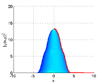
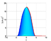
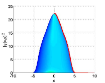
Figure 10: Simulation results (density distributions, blue) and comparison with the collocation method (red line) for $R=2$ (left), $R=3$ (center), and $R=4$ (right).

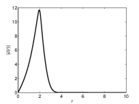
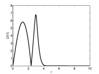
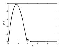
Figure 11: Magnitude of the current $J$ corresponding to the solutions for $R=2$ (left), $R=3$ (center), and $R=4$ (right).

For $R=5$, the solution becomes unstable, as predicted in Section 3. Fig. 12 shows the corresponding transient that, after breaking the symmetry, leads to the emergence of vortex lattices. These vortex lattices remain rotating at a constant angular velocity, becoming the stable solution of the system. (This simulation is also presented in the supplementary videos Sim1.avi and Sim2.avi.) Furthermore, Figs. (14) to (17) show the characteristics of these quantum vortices: the density profile drops to zero at the center of the vortex core, as shown in Fig. 14; the phase difference around the vortex is a multiple of $2\pi$, as seen in Fig. 15 (left), where there is a change in the phase from $0$ to $2\pi$ in all the vortices (indicated with blue circles); the condensate circulates around the vortex, as depicted in Fig. 16, where the current $J$ is plotted for a central vortex (left) and a satellite vortex (right). Finally, Fig. (17) shows the plot of $\left|\nabla\theta\right|$, the magnitude of the gradient of the phase, which is proportional to the velocity of the condensate. Notice that $\left|\nabla\theta\right|\approx 1/r$ around the core of the vortices. Finally, Fig. (18) shows the results for $R=6,7,8,9$.

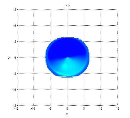
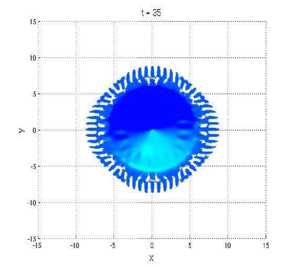
Figure 12: Simulation results for $R=5$ (see also the supplementary videos Sim1.avi and Sim2.avi). The plots show the density distribution at different times (continued in Fig. (13)). The white areas represent regions where the density becomes zero. At the beginning, the condensate is confined in a radius approximately equal to 5. After breaking of symmetry, the condensate cloud experiences an expansion, and the remnants of this expansion can be seen at $R\gtrsim 5$. Notice that the white dots inside the region $R\lesssim 5$ at $t=70$ correspond to the vortices that will eventually form the stable lattice. Some of these vortices are expelled out of the structure during the transient evolution.

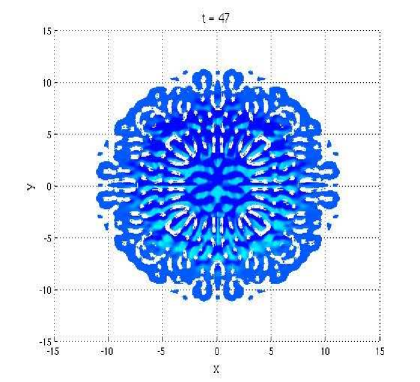
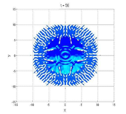
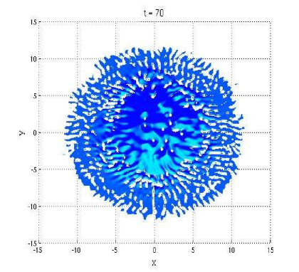
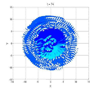
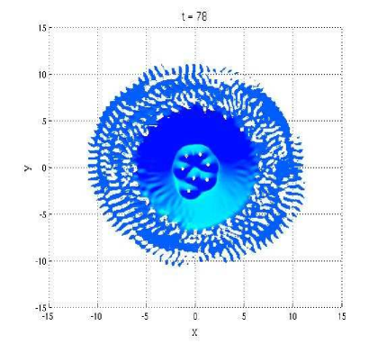
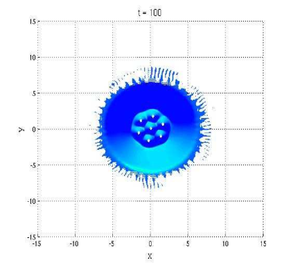
Figure 13: Continuation of Fig. (12).

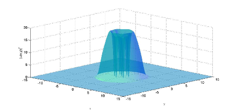
Figure 14: A transparent image corresponding to the density distribution at $t=140$ ($R=5$).

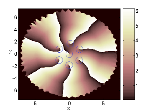
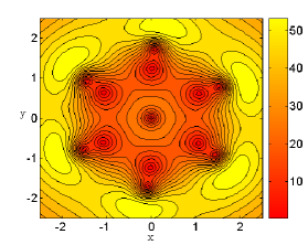
Figure 15: Left: Phase $\theta(x,y)$ of the solution at $t=140$ ($R=5$), with the blue circles indicating the core of the vortices. Right: The magnitude of the current$\left|J\left(x,y\right)\right|$ at $t=140$. Notice that the contour lines are closer around the core of the vortices.

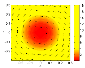
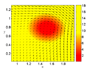
Figure 16: Density distribution and arrows corresponding to the current $J$ in the central vortex (left) and one satellite vortex (right) of the solution at $t=140$ ($R=5$).

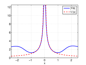
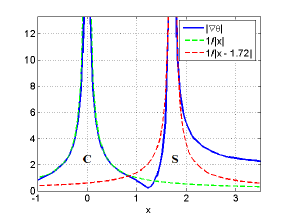
Figure 17: 1D plot for $\left|\nabla\theta\right|$ ($R=5$): central vortex (left); central vortex “C” and satellite vortex “S” (right). For both central and satellite vortices, $\left|\nabla\theta\right|\approx 1/\left|x\right|=1/r$ around the cores.

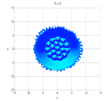
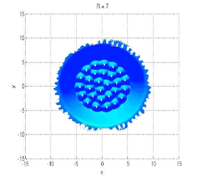
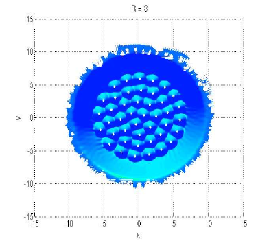
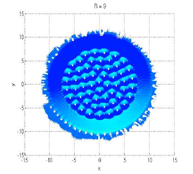
Figure 18: Vortex lattices for $\alpha=4.4$, $\sigma=0.3$ and different values of $R$.

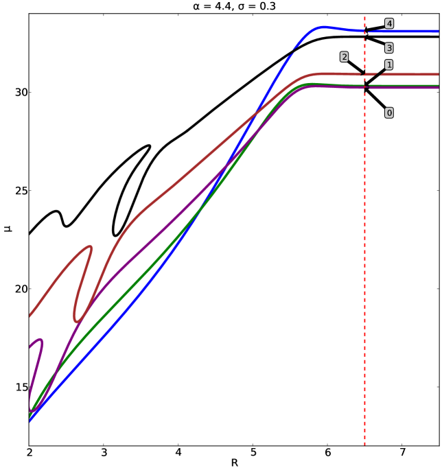
Figure 19: Continuation in $R$ starting from the solutions displayed in Figs. 8 and 9. The density profiles corresponding to the points labeled 0 to 4 are shown in Fig 20.

6.2 Numerical continuation in $R$

Figure (19) shows the continuation in $R$ starting from the solutions displayed in Figs. (8) and (9). It can be seen that for all the branches, the solutions remain unchanged for large values of $R$. Moreover, the blue branch, which corresponds to the branch studied in the linear stability analysis performed in Section 4, has the smallest $\mu$ up to $R\simeq 4.4$. This is also the point at which the branch becomes linearly unstable, as shown in Fig. (5). On the other hand, Fig. (20) shows the density profiles corresponding to the solutions labeled 0 to 4 in Fig. (19). Notice that although the continuation process started in the multi-bump profiles shown in Figs. (8) and (9), these solutions do not have this multi-bump characteristic. Also, the blue branch is not the one with the smallest $\mu$ for large values of $R$. In any case, for large values of $R$, none of these radially symmetric solutions is linearly stable. It is interesting to observe that even though the radially symmetric solutions remain unchanged for large values of $R$, the stable vortex lattice solutions change as $R$ increases, as seen in Fig. (18).

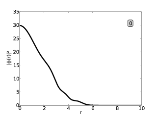
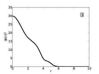
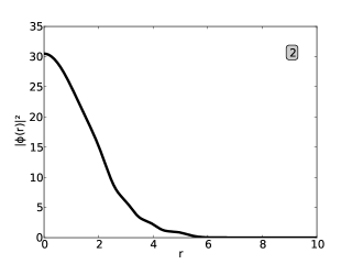
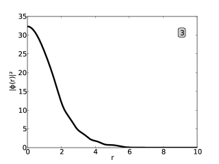
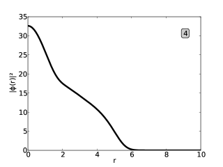
Figure 20: Density profiles corresponding to the solutions labeled 0 to 4 in Fig. 19.

6.3 Central vortex states

Let us now investigate the existence of central vortex states similar to the ones observed in a rotating BEC [8]. To find these states, consider solutions of (1) of the form $\psi\left(x,t\right)=e^{-i\mu t}\psi_{m}\left(x\right)=e^{-i\mu t}\psi_{m}\left(r\right)e^{im\theta}$, where $\mu$ is the chemical potential and $m=1,2,3,...$ is called the winding index. Introducing this ansatz into (1) gives the following expression for $\psi_{m}$:

$$\mu\psi_{m}\left(r\right)=\left[-\frac{1}{r}\frac{d}{dr}\left(r\frac{d}{dr}\right)+\frac{m^{2}}{r^{2}}+V(r)+\left|\psi_{m}\left(r\right)\right|^{2}+i\left(\alpha\Theta_{R}-\sigma\left|\psi_{m}\left(r\right)\right|^{2}\right)\right]\psi_{m}\left(r\right),$$ (44)

with

$$\begin{array}[]{ccc}\psi{}_{m}\left(0\right)=0,&&\lim_{r\rightarrow\infty}\psi_{m}\left(r\right)=0\end{array}.$$

This problem is solved by the collocation method described in Section 3. Figure 21 shows the results for $\alpha=4.4$, $\sigma=0.3$, $R=5$ and $m=1$ to $8$. To study their linear stability, small perturbations of the wave function can be expressed as

$$\begin{array}[]{cc}\psi\left(r,\theta,t\right)=e^{-i\mu t}\left[\psi_{m}\left(r\right)e^{im\theta}+\varepsilon\left(u(r)e^{i\left(n\theta-\omega t\right)}+v^{*}\left(r\right)e^{i\left(n\theta+\omega^{*}t\right)}\right)\right],&n=1,2,...,\end{array}$$ (45)

with $\varepsilon\rightarrow 0$. The perturbation is time dependent with frequency $\omega$ and the complex amplitude functions $u(r)$ and $v\left(r\right)$. Proceeding as in the linear stability analysis performed in Section 4 with $n=1,...,50$, it can be shown that all of the central vortex states displayed in Fig. (21) are linearly unstable. When these central vortex states are used as initial conditions for the Strang-splitting spectral method, it is possible to study the manifestation of these instabilities. In particular, Figs. (22) and (23) show the results for $m=1,2$. The $m=1$ vortex remains for a long time, and then it undergoes symmetry breaking and gives rise to a vortex lattice. The $m=2$ vortex has an additional interesting behavior: it remains for a short time; the vortex then splits into two $m=1$ vortices; and finally this solution breaks and generates a vortex lattice. The splitting for the case $m=2$ was observed experimentally in [30] in an exciton-polariton condensate.

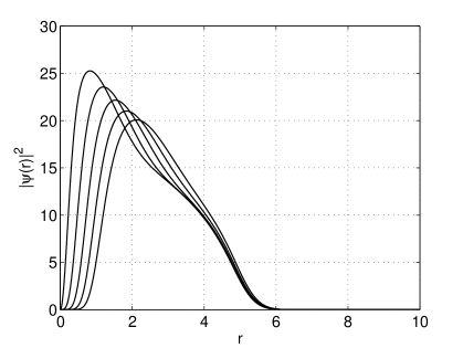
Figure 21: Density distributions corresponding to the central vortex states for $\alpha=4.4$, $\sigma=0.3$, $R=5$ and $m=1$ to 5 (in order of decreasing peaks).

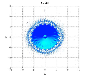
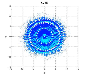
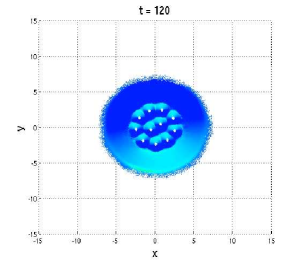
Figure 22: Simulation result for the $m=1$ central vortex state (see also supplementary video Sim3.avi).

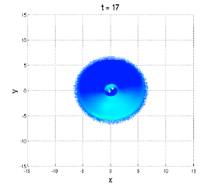
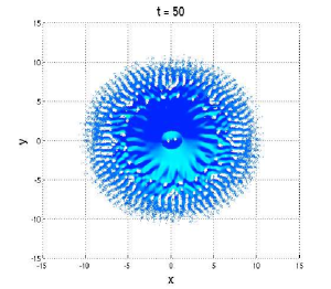
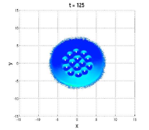
Figure 23: Simulation result for the $m=2$ central vortex state (see also supplementary video Sim4.avi).

7 Conclusions

The general behavior of the 2D complex GP equation was presented using different numerical techniques. The first step for the numerical characterization of this equation was the analysis of its radially symmetric solutions. Due to the lack of conservation of mass and energy, the standard techniques used for the study of the radially symmetric ground state solution of the GP equation, such as the gradient flow method, do not apply in this case. In order to overcome this problem, the stationary complex GP equation (3) was studied directly using a collocation method. Once the radially symmetric solutions were obtained, their linear stability was investigated. Afterwards, numerical continuation was applied to one of the linearly stable solutions to study its excited states. We found that the linearly stable solution has the smallest chemical potential in the group of solutions found, which leads us to define it as the ground state of the system and the rest of the solutions as excited states. However, a rigorous definition of the energy is required to corroborate this statement.

We used numerical integration to study the nonlinear evolution of the linearly unstable solutions. We observed the emergence of complicated vortex lattices after symmetry breaking (this fact was also shown by Keeling and Berloff [25]). These lattices remain rotating with a constant angular velocity, becoming the stable solution of the system.

Finally, we computed the central vortex solutions of the complex GP equation. An interesting result was the splitting of the $m=2$ central vortex into two $m=1$ vortices, which was observed experimentally by Sanvitto et al. [30] in a Bose-Einstein condensation of exciton-polaritons. From all this, it is possible to see the rich behavior of the complex GP equation, which in some way combines the characteristics of both the GP and the complex Ginzburg-Landau equations.

8 Acknowledgments

The first author acknowledges the assistance and comments from D. Ketcheson, P. Antonelli, N. Berloff, B. Sandstede, B. Oldeman and the Research Computing Group from KAUST. The work of the last author has been supported by the Hertha-Firnberg Program of the FWF, grant T402-N13.

9 References

References

- A. and M. [2013] Bramati A. and Modugno M. Physics of Quantum Fluids. New Trends and Hot Topics in Atomic and Polariton Condensates. Springer, 2013.
- Anderson et al. [1995] M. Anderson, J. Ensher, M. Matthews, C. Wieman, and E. Cornell. Observation of Bose–Einstein condensation in a dilute atomic vapor. Science, 269(5221):198–201, 1995.
- Antonelli et al. [2013] P. Antonelli, R. Carles, and C. Sparber. On nonlinear Schrödinger type equations with nonlinear damping. arXiv preprint arXiv:1303.3033, 2013.
- Ascher et al. [1987] U.M. Ascher, R.M. Mattheij, and R.D. Russell. Numerical solution of boundary value problems for ordinary differential equations, volume 13. Society for Industrial and Applied Mathematics, 1987.
- Bao et al. [2002] W. Bao, S. Jin, and P.A. Markowich. On time-splitting spectral approximations for the Schrödinger equation in the semiclassical regime. Journal of Computational Physics, 175(2):487–524, 2002. ISSN 0021-9991.
- Bao et al. [2003] W. Bao, D. Jaksch, and P.A. Markowich. Numerical solution of the Gross-Pitaevskii equation for Bose-Einstein condensation. Journal of Computational Physics, 187(1):318–342, 2003. ISSN 0021-9991.
- Bao et al. [2004] W. Bao, D. Jaksch, and P.A. Markowich. Three-dimensional simulation of jet formation in collapsing condensates. Journal of Physics B: Atomic, Molecular and Optical Physics, 37(2):329, 2004.
- Bao et al. [2005] W. Bao, H. Wang, and P.A. Markowich. Ground, symmetric and central vortex states in rotating Bose-Einstein condensates. Communications in Mathematical Sciences, 3(1):57–88, 2005.
- Borgh et al. [2012] M. Borgh, G. Franchetti, J. Keeling, and N. Berloff. Robustness and observability of rotating vortex lattices in an exciton-polariton condensate. Physical Review B, 86(3):035307, 2012.
- Bose [1924] S. Bose. Plancks gesetz und lichtquantenhypothese. Z. phys, 26(3):178, 1924.
- Bradley et al. [1995] C. Bradley, C. Sackett, J. Tollett, and R. Hulet. Evidence of Bose–Einstein condensation in an atomic gas with attractive interactions. Physical Review Letters, 75(9):1687, 1995.
- Brunner [2004] H. Brunner. Collocation methods for Volterra integral and related functional differential equations, volume 15. Cambridge University Press, 2004.
- Coldren and Corzine [1995] L. Coldren and S. Corzine. Diode lasers and photonic integrated circuits, volume 218. Wiley Series in Microwave and Optical Engineering, 1995.
- Cuevas et al. [2011] J. Cuevas, A.S. Rodrigues, R. Carretero-González, P.G. Kevrekidis, and D.J. Frantzeskakis. Nonlinear excitations, stability inversions, and dissipative dynamics in quasi-one-dimensional polariton condensates. Physical Review B, 83(24):245140, 2011.
- Davis et al. [1995] K. Davis, M. Mewes, M. Andrews, N. van Druten, D. Durfee, D. Kurn, and W. Ketterle. Bose–Einstein condensation in a gas of sodium atoms. Physical Review Letters, 75(22):3969–3973, 1995.
- De Hoog and Weiss [1976] F.R. De Hoog and R. Weiss. Difference methods for boundary value problems with a singularity of the first kind. SIAM Journal on Numerical Analysis, 13(5):775–813, 1976.
- Doedel et al. [2007] E.J. Doedel, R.C. Paffenroth, A.R. Champneys, T.F. Fairgrieve, Y.A. Kuznetsov, B.E. Oldeman, B. Sandstede, and X.J. Wang. Auto-07p: Continuation and bifurcation software for ordinary differential equations (2007). Available for download from http://indy.cs.concordia.ca/auto, 2007.
- Einstein [1924] A. Einstein. Sitzungsberichte der preussischen akademie der wissenschaften. Physikalisch-mathematische Klasse, 261(3), 1924.
- Einstein [1925] A. Einstein. Quantum theory of the monoatomic ideal gas. Sitzungsber. Preuss. Akad. Wiss, page 261, 1925.
- Gasser and Markowich [1997] I. Gasser and P. Markowich. Quantum hydrodynamics, Wigner transforms, the classical limit. Asymptotic Analysis, 14(2):97–116, 1997.
- Govaerts [2000] W.J.F. Govaerts. Numerical methods for bifurcations of dynamical equilibria. Number 66. SIAM, 2000.
- Gross [1963] E. Gross. Hydrodynamics of a superfluid condensate. Journal of Mathematical Physics, 4:195, 1963.
- Kasprzak et al. [2006] J. Kasprzak, M. Richard, S. Kundermann, A. Baas, P. Jeambrun, J. Keeling, Marchetti F., M. Szymanacute, R. Andre, and Staehli. Bose–Einstein condensation of exciton polaritons. Nature, 443(7110):409–414, 2006.
- Keeling and Berloff [2011] J. Keeling and N. Berloff. Exciton–polariton condensation. Contemporary Physics, 52(2):131–151, 2011.
- Keeling and Berloff [2008] J. Keeling and N.G. Berloff. Spontaneous rotating vortex lattices in a pumped decaying condensate. Physical review letters, 100(25):250401, 2008. ISSN 1079-7114.
- Keller [1977] H.B. Keller. Numerical solution of bifurcation and nonlinear eigenvalue problems. Applications of bifurcation theory, pages 359–384, 1977.
- Keller [1987] H.B. Keller. Lectures on numerical methods in bifurcation problems. Applied Mathematics, 217:50, 1987.
- Pitaevskii [1961] L. Pitaevskii. Vortex lines in an imperfect Bose gas. Sov. Phys. JETP, 13(2):451–454, 1961.
- Pitaevskii and Stringari [2003] L. Pitaevskii and S. Stringari. Bose-Einstein Condensation. Number 116. Oxford University Press, 2003.
- Sanvitto et al. [2010] D. Sanvitto, F. M. Marchetti, M. H. Szymanska, G. Tosi, M. Baudisch, F.P. Laussy, D.N. Krizhanovskii, M.S. Skolnick, L. Marrucci, A. Lemaitre, J. Bloch, C. Tejedor, and L. Vina. Persistent currents and quantized vortices in a polariton superfluid. Nature Physics, 2010. ISSN 1745-2473.
- Wouters and Carusotto [2007] M. Wouters and I. Carusotto. Excitations in a nonequilibrium Bose–Einstein condensate of exciton polaritons. Physical review letters, 99(14):140402, 2007.