Bulk effects on topological conduction on the surface of 3-D topological insulators

Abstract

The surface states of a topological insulator in a fine-tuned magnetic field are ideal candidates for realizing a topological metal which is protected against disorder. Its signatures are (1) a conductance plateau in long wires in a finely tuned longitudinal magnetic field and (2) a conductivity which always increases with sample size, and both are independent of disorder strength. We numerically study how these experimental transport signatures are affected by bulk physics in the interior of the topological insulator sample. We show that both signatures of the topological metal are robust against bulk effects. However the bulk does substantially accelerate the metal’s decay in a magnetic field and alter its response to surface disorder. When the disorder strength is tuned to resonance with the bulk band the conductivity follows the predictions of scaling theory, indicating that conduction is diffusive. At other disorder strengths the bulk reduces the effects of surface disorder and scaling theory is systematically violated, signaling that conduction is not fully diffusive. These effects will change the magnitude of the surface conductivity and the magnetoconductivity.

I Introduction

The Dirac fermions residing on the surface of strong topological insulators (TIs) provide a new opportunity for realizing a topological metal which remains conducting regardless of disorder strength or sample size. Kane and Mele (2005); Min et al. (2006); Zhang et al. (2009); Hasan and Kane (2010); Li et al. (2012); Culcer (2012); Bardarson and Moore (2013) This metal should be general to any single species of Dirac fermions which breaks spin symmetry but retains time reversal symmetry. When the Fermi level is tuned inside the TI’s bulk band gap, all states inside the TI bulk are localized. Conduction can occur only on the TI surface, which hosts a single species of two-dimensional (2-D) Dirac fermions. These are predicted to remain always conducting regardless of disorder strength, forming a topological metal.

Many beautiful TI experiments have visualized the Dirac cone, spin-momentum locking, Landau levels with $\sqrt{n}$ spacing, and SdH oscillations. Hsieh et al. (2008); Hanaguri et al. (2010) These signals are visible only when either momentum or the Landau level index are approximately conserved; they disappear when disorder is strong. In contrast, the topological metal’s hallmark is robust surface conduction at any disorder strength and in large samples, even when disorder destroys the Dirac cone. In this article we will focus on experimental signatures of this protection against disorder.

We will show that bulk physics in the TI’s interior substantially modifies the topological metal. Even though it is a surface state, in response to disorder it may explore the TI bulk or even tunnel between surfaces. We used several months on a large parallel supercomputer to perform extensive calculations of conduction, including both bulk and surface physics.

Two experimental signatures are available for proving incontrovertibly that a topological metal is indeed robust against disorder. The first is a quantized conductance in long wires. In ordinary wires the conductance $G$ decreases with wire length until only one channel remains open, i.e. $G=\frac{e^{2}}{h}$, and then transits into a localized phase where the last channel decays exponentially. In contrast the topological metal exhibits one perfectly conducting channel (PCC) which remains forever topologically protected, so in long wires the conductance is quantized at $G=\frac{e^{2}}{h}$. Zirnbauer (1992); Mirlin et al. (1994); Ando and Suzuura (2002); Takane (2004); Ryu et al. (2007); Ostrovsky et al. (2010); Zhang and Vishwanath (2010); Hong et al. (2013) The PCC can be realized only when there is no gap in the surface states’ Dirac cone. In TI wires locking between spin and momentum creates a gap, but a specially tuned longitudinal magnetic field $B$ can be used to close the gap and realize the PCC’s quantized conductance. In this fine-tuned scenario $B$ breaks time reversal symmetry and causes the PCC to eventually decay. Our results will confirm the PCC’s robustness against bulk effects, and show that both the optimal value of $B$ and the PCC’s optimal decay length are altered by bulk physics. These results, and the PCC’s response to sample dimensions, magnetic fields, and disorder, will be useful to experimental PCC hunters.

The second key signature of the topological metal concerns the diffusive regime, where the sample aspect ratio $L/W$ is small enough that several conducting channels remain open, but the sample is still bigger than the scattering length. ($W$ and $L$ are the sample width and length.) In this regime, regardless of disorder strength, a topological metal’s conductivity $\sigma=GL/W$ always increases when the length $L$ and width $W$ are increased in proportion to each other. Ostrovsky et al. (2007); Nomura et al. (2007); Bardarson et al. (2007); San-Jose et al. (2007); Tworzydlo et al. (2008); Lewenkopf et al. (2008); Adam et al. (2009); Mucciolo and Lewenkopf (2010); Mong et al. (2012) This signature contrasts with non-topological materials where the conductivity can always be forced to decrease by making the disorder large enough. Asada et al. (2004); Nomura et al. (2007) In both cases the increasing conductivity - called weak antilocalization (WAL) - can be removed by introducing a weak magnetic field; experimental studies of the TI magnetoconductivity are extremely popular. In the diffusive regime both the conductivity and the magnetoconductivity are expected to follow universal curves prescribed by scaling theory, independent of sample details.

Here we will confirm that the always-increasing conductivity is robust against both bulk effects and very strong disorder. We will also show that the bulk reduces scattering and causes violation of the universality predicted by scaling theory, which implies that the topological metal’s conduction is not purely diffusive. This has immediate consequences for experiments: we expect that magnetoconductivity measurements are sensitive to bulk physics, and that the magnitude of the observed signal will vary systematically with the Fermi level and disorder strength.

Lastly, we find that the bulk reduces the effects of scatterers residing on the TI surface. The topological metal is free to reroute around scatterers, into the TI bulk. This is a second level of topological protection, in addition to the well-known suppression of backscattering. It should change the surface conductivity and increase the topological metal’s robustness against issues of sample purity, substrates, gating, etc.

II The Model

The topological metal is independent of any short-scale variation in the TI sample, including any microscopic details of the Hamiltonian. Its two signatures are regulated by only two parameters: the scattering length and localization length. Because we are concerned with Fermi energies inside the bulk band gap, bulk effects on the topological metal can depend on only a small number of parameters - the Fermi level, the Fermi velocity, the penetration depth, the bulk band gap, and the bulk spectral width. Therefore we study a computationally efficient minimal tight binding model of a strong TI implemented on a cubic lattice with dimensions $H,W$, and $L$. With four orbitals per site, the model’s momentum representation is:

$$\mathcal{H}(\vec{k}) = 2\Gamma^{1}-\frac{1}{2}\sum_{i=1}^{3}(\Gamma^{1}-\imath\Gamma^{i+1})e^{-\imath k_{i}a}+H.c.$$ (1)

$\Gamma^{i}$ are the Dirac matrices $1\otimes\sigma_{z},-\sigma_{y}\otimes\sigma_{x},\sigma_{x}\otimes\sigma_{x},-1\otimes\sigma_{y}$, $a=1$ is the lattice spacing, and the penetration depth is $d\propto a$. Schubert et al. (2012) We include a magnetic field oriented longitudinally along the axis of conduction by multiplying the hopping terms by Peierls phases. This non-interacting model exhibits a spectral width $\Delta E=10$, a bulk band gap in the interval $E=[-1,1]$, a single Dirac cone in the bulk gap, and Fermi velocity $v_{F}=2$. To this model we add uncorrelated white noise disorder $u(x)$. On each individual site the disorder is proportional to the identity and its strength is chosen randomly from the interval $\left[-U/2,\,U/2\right]$, where $U$ is the disorder strength. We attach two clean semi-infinite leads that have $W\times H$ cross-sections equal to that of the sample itself and evaluate the conductance using the Caroli formulaCaroli et al. (1971); Meir and Wingreen (1992) $G=-\frac{e^{2}}{h}{Tr}((\Sigma^{r}_{L}-\Sigma^{a}_{L})G^{r}_{LR}(\Sigma^{r}_{R}-\Sigma^{a}_{R})G^{a}_{RL})$. $G^{a},G^{r}=(E_{F}-\mathcal{H}-u\mp\imath\epsilon)^{-1}$ are the advanced and retarded single-particle Green’s functions connecting the left and right leads, and $\Sigma_{L,R}$ are the lead self-energies. Sancho et al. (1985)

In our study we will leave the TI bulk pure, since the main effects of bulk disorder on the surface states can be duplicated by adjusting the bulk parameters. In particular, the bulk band width widens, the bulk band gap narrows, and the penetration depth increases. These parameters are only weakly sensitive to disorder when the disorder is small compared to the band width. When the disorder strength approaches the band width the bulk states gradually delocalize, surface states are eventually destroyed by tunneling through the bulk, and the material ceases to be a TI. Groth et al. (2009); Guo et al. (2010); Chen et al. (2012); Xu et al. (2012); Kobayashi et al. (2014) In contrast our focus here is on bulk effects on a healthy topological metal, which are controlled only by the few bulk parameters which we have listed. We include only surface disorder, which has been extensively investigated experimentally because practical TI devices may be capped, gated, bombarded, or left exposed to atmosphere. Analytis et al. (2010); Brahlek et al. (2011); ValdesAguilar et al. (2012); Tereshchenko et al. (2011); Hsieh et al. (2009); Noh et al. (2011); Liu et al. (2012); Lang et al. (2011); Chen et al. (2010); Kong et al. (2011)

III The Perfectly Conducting Channel

In Figures 1 and 2 we focus on the topological metal’s PCC signature, which is a quantized conductance plateau seen in very long samples. We set the disorder strength to $U=2$, and the Fermi energy is $E_{F}=0.7$ in both the sample and the leads. Figure 1a shows the plateau in $W\times H$ slabs, which retain all bulk physics but are simplified by avoiding the gap in the surface Dirac cone. The plateau conductance is $G=2\frac{e^{2}}{h}$ because each surface hosts a PCC. We define the PCC decay length $\lambda$, i.e. the plateau length, as the wire length where the conductance is half of its plateau value. Figure 1c shows that $\lambda$ grows exponentially as the slab height $H$ increases from $3$ to $8$, which proves that the PCC decay is caused by tunneling and is exponentially small except in very thin slabs. Wu et al. (2013) This is disorder-enabled tunneling; $\lambda$ diverges in pure slabs.

Figure 1: (Color online.) The perfectly conducting channel (PCC), a topologically protected conductance plateau in very long TI samples. (a,b) The conductance plateau as a function of length $L$ in (a) $W\times H$ slabs with no magnetic field, and in (b) $W\times W$ wires with a fine-tuned longitudinal field. (c) In slabs the decay length $\lambda$ is controlled by tunneling and scales exponentially with slab height $H$. (d) In wires the decay length scales with $W^{3}$ and is caused by the surface state’s penetration into the bulk. The dotted lines are (c) $\lambda\propto\exp(1.12\;H)$ and (d) $\lambda=4W^{3}$.

Next we turn to $W\times W$ TI wires, where the PCC is realized only after we remove the gap in the Dirac cone. Since spin is locked to momentum in TIs, parallel transport of the spin on one circuit around a wire’s circumference causes a $\pi$ Berry phase. This causes a small gap $\Delta_{B}=2\sqrt{2}v_{F}/C$ where $C$ is the wire circumference. However the $\pi$ phase can be canceled and the gap removed if the magnetic flux through the wire is fine-tuned to produce an additional $\pi$ phase. Ostrovsky et al. (2010); Rosenberg et al. (2010); Egger et al. (2010); Zhang and Vishwanath (2010); Bardarson et al. (2010) Figure 1b shows our results after numerically optimizing $B$ to maximize the PCC lifetime, which at leading order kept the magnetic length $L_{B}\propto\sqrt{\hbar/eB}$ proportional to the wire width $W$. The obvious PCC conductance plateau confirms that the topological metal is robust in wires.

Figure 1d presents the first numerical calculations of the PCC decay length $\lambda$’s dependence on the wire width $W$ in a model which includes the TI bulk. Our results are of high accuracy, with errors of a few percent. They required calculation of very long and wide wires, numerical optimization of $B$, and many samples (from $N=864$ for $W\leq 12$ to $N=80$ for $W=18$). They prove that PCC decay in wires is much faster than a slab’s exponentially slow decay, and that $\lambda$ scales with the cube of the wire width $\lambda\approx\alpha W^{3}$, with prefactor $\alpha\approx 4$. This points to the magnetic field and not tunneling as the dominant source of PCC decay in TI wires.

The decay length’s cubic $W^{3}$ scaling is caused by bulk physics. Previously $\lambda\propto W^{4}$ scaling was predicted based on a bulk-independent mechanism Zhang and Vishwanath (2010); Ando (2006). Diffusion into the bulk Altshuler and Aronov (1981) is also expected to scale with $L_{B}^{4}\propto W^{4}$. If we note that the large value of $\alpha$ prohibits instances of the inverse scattering length $l^{-1}\approx 1/30a$ (see the supplemental material), then simple dimensional analysis obtains $\lambda\propto W^{3}/d^{2}$, where $d\propto a$ is the penetration depth of the surface states. This implies that the fastest mechanism of PCC decay is caused by the surface state’s penetration into the bulk.

Figure 2: (Color online.) The conductance plateau’s dependence on magnetic field $B$ at disorder strength $U=2$. The wire lengths of the $20\times 20$ wires (right pane) are chosen to be about $8$ times bigger than the wire lengths of the $10\times 10$ wires (left pane). On the ${x}$ axis we plot the magnetic field, rescaled by $W/4B_{0}\propto W^{3}$. The match between the $10\times 10$ and $20\times 20$ wires proves that the decay length scales with $W^{3}$ and that the conductance peak’s width (in $B$) scales with $W^{-3}$. At $U=2$ bulk effects cause the conductance peak to shift to a larger field strength, so we have subtracted from $B$ the optimal field strength $B_{0}$ at zero disorder.

Bulk physics also combines with surface disorder to alter the magnetic field strength which maximizes $\lambda$. In any TI disorder on the surface will push the topological states into the bulk, rescaling their magnetic cross-section by $(1-4\delta/W)$. Schubert et al. (2012); Wu et al. (2013); Dufouleur et al. (2013) $\delta$ is their displacement, which can be determined from the shift in optimal magnetic field via $\delta=(B_{opt}-B_{0})(W/4B_{0})$, where $B_{opt}$ and $B_{0}$ are respectively the optimal fields at finite disorder $U$ and at zero disorder $U=0$. Figure 2 plots the conductance at $U=2$ as a function of $\delta B\,(W/4B_{0}),\;\delta B=B-B_{0}$. It shows that the displacement at $U=2$ is about $0.06$ lattice units and the change in optimal field is $B_{opt}-B_{0}=0.24\,B_{0}/W$.

The two panes of Figure 2 show that after rescaling by $W/4B_{0}$ the conductance peak has the same position and width in both $10\times 10$ and $20\times 20$ wires. This proves that both the optimal value and the peak width of the magnetic field scale with $B_{0}\delta/W\propto W^{-3}$. In thick wires the PCC will not be visible unless the magnetic field is very finely tuned with an accuracy proportional to $W^{-3}$. We expect that this formula, the previous scaling formulas, and the graphs of the PCC peak will all be useful for PCC hunters.

Figure 3: (Color online.) The conductivity $\sigma$ and its logarithmic derivative $\beta(L)=d\ln\sigma/d\ln L$. (a) Convergence of $\beta$ and $\sigma$ (in inset) as the sample width $W$ is increased from $15$ to $80$. (c) The resonance between the topological surface state and the bulk band, manifested as valleys in both $\beta$ (solid lines) and $2/\pi\sigma$ (dashed lines). At the resonance center the topological state is most strongly disordered, and also exhibits the largest conductivity. (b) Topological protection ensures that the surface states’ conductivity $\sigma$ always increases with sample size $L$, as verified here near the resonance center $U=7.2$, off-center $U=9.1$, and in the large-disorder shoulder $U=15.9,30.0$. At very small $L$ tunneling through the bulk causes $\sigma$ to decrease with $L$. The variation in line slope with $U$ and with Fermi energy $E_{F}$ breaks the universality predicted by scaling theory. (d) The $\beta$ function. Scaling theory predicts a universal $\beta=2/\pi\sigma$ curve independent of $U$ and $E_{F}$, shown here as a black dotted-dashed curve, and also shown in pane (a). The deviations from universality seen here imply similar behavior in the magnetoconductivity.

IV The Conductivity

In Figure 3 we turn to studying the topological metal’s second signature, a conductivity $\sigma$ which grows robustly with sample size regardless of disorder strength. We have carefully controlled for many effects and errors. $\sigma$ grows only in the diffusive regime where several channels remain conducting, and here it is independent of sample width $W$. Figure 3a shows that both $\sigma$ and its logarithmic derivative $\beta(L)=d\ln\sigma/d\ln L$ converge to their diffusive values when $W>1.1\,L$; we restrict our remaining data to this converged regime. Moreover in the diffusive regime both large slabs and large wires have the same conductivity; the gap is erased by disorder, and has no effect even at $E=0$. (See the supplemental material.) Here we report results obtained from slabs. We also ensure convergence with slab height $H$ by using thick slabs with $H=6$ in Figure 3a and $H=12$ elsewhere. The associated computational cost is compounded by $\beta$’s sensitivity to statistical errors; very large $N=960-4800$ numbers of samples - and smoothing in panes (a) and (c) - were necessary to obtain these low-noise $\beta$ curves. Leads effects are minimized by doping them into the metallic bulk band at $E_{F}=2$.

The most prominent feature of our data is highlighted in Figure 3c: a resonance between the disordered surface states and the bulk band, seen here as a valley in both $2/\pi\sigma$ and $\beta$, which we have plotted as functions of disorder $U$ at four Fermi levels inside the gap. It is centered around disorder strength $U=[6,10]$, matching the bulk band width $\Delta E=10$. The resonance is generic to all TIs, since its physics is generic: surface disorder displaces the surface states into the bulk, as we already saw in Figure 2. At weak disorder $U$ the displacement is small ($\delta=0.06$ at $U=2$ in our model), but as $U$ passes through the resonance center the surface states migrate from the disordered surface layer into the clean bulk. At the resonance center scattering is maximized, as is mixing between the bulk and the surface states. Since quantum scattering processes are responsible for the conductivity’s growth, $\sigma$ is also maximized at the resonance center. We conclude that outside the resonance center the bulk tends to decrease the effect of surface disorder. This will change the magnitude of the surface conduction in TI samples and will also change the scattering length and the diffusion constant, each of which can be observed experimentally.

Figure 3c shows a very interesting feature: at the resonance center the four conductivity curves kiss, which signals that scattering is independent of energy. The surface density of states (DOS) $\rho$ also must be independent of energy, since it determines the scattering time via $\tau\propto(\langle U^{2}\rangle\,\rho)^{-1}$. This is in remarkable contrast with the linear DOS $\rho(E)\propto E$ seen at zero disorder.

Figure 3b examines the the conductivity growth signature of topological metals at two values of the Fermi level $E_{F}=0,\,0.2$ and four representative disorder strengths. The growth is very clear in the two pink lines at the top which lie near the resonance center $U=7.2$, and also in the slightly lower two orange lines which lie slightly off-center $U=9.1$. The lowest four lines lying in the resonance shoulder $U=15.9,\,30.0$ do reveal a decreasing conductivity at small $L$, but this is a finite-size effect from the leads: disorder-assisted bulk tunneling between the leads increases $\sigma$ in very short samples, and this excess decreases rapidly with $L$. (See the supplemental material.) Leaving aside this tunneling effect, we find that $\sigma$ grows even when its value (per surface) is as small as $\sigma\geq 0.31\frac{e^{2}}{h}\approx\frac{1}{\pi}\frac{e^{2}}{h}$. This contrasts with materials without topological protection where any value of $\sigma$ up to $\sigma_{C}\approx 1.4\frac{e^{2}}{h}$ produces a decreasing conductivity Kawarabayashi and Ohtsuki (1996); Kawabata (2003); Asada et al. (2004, 2006); Markos and Schweitzer (2006); Nomura et al. (2007), and proves that a TI’s conductivity growth is robust against bulk effects.

The details of Figure 3 can be compared with the one parameter scaling theory of conduction, which makes specific predictions about the diffusive regime. Scaling theory’s most important prediction is universality: the only effect of changing the disorder strength and Fermi level should be to rescale both the scattering length $l$ and the overall length scale. Abrahams et al. (1979) The $\beta$ function is not sensitive to $l$, so it should be universal. Numerical works on topological metals have shown that this universal curve agrees quite well with $\beta(\sigma)=1/\pi\sigma$, even when $\sigma\approx 1/\pi$ is quite small. Hikami et al. (1980); Bardarson et al. (2007); Nomura et al. (2007); Mucciolo and Lewenkopf (2010) In consequence $\sigma$ grows logarithmically $\propto 1/\pi\;\ln L$. In our TI slabs $\beta$ and $\sigma$ are multiplied by $2$ for the two surfaces. In summary, scaling theory predicts that in Figure 3d the $\beta(\sigma)$ curves should all coincide with each other and with the $2/\pi\sigma$ black dotted line, and that in Figure 3c each solid $\beta(\sigma)$ line should coincide with its partnering dashed $2/\pi\sigma$ line. Moreover the conductivity curves in Figure 3b should all follow straight lines with the same slope $2/\pi$. These universal results are at the origin of the Hikami-Larkin-Nagaoka formula which gives a universal prediction for the conductivity’s response to a small magnetic field, and in particular the $2/\pi$ coefficient in these scaling theory predictions transfers over directly to the HLN formula’s magnitude. Hikami et al. (1980)

Near the resonance center $U\approx 7.2$ we find excellent agreement with scaling theory, as evidenced by the pink straight line conductivity curves found in Figure 3b and by the pink $\beta$ curves in Figure 3d which coincide nicely with $2/\pi\sigma$. The excellent agreement with scaling theory indicates that at the resonance center conduction is completely determined by diffusion and its quantum corrections, and that the scattering length is very small.

At other disorder strengths we find that scaling theory’s universality is systematically violated. We begin well within the resonance at $U=9.1$, which is shown in the orange lines in Figures 3b,d. These lines are straight, indicating that the conductivity grows with the dimensionless quantity $\ln L$, and proving that $\sigma$ is not controlled by any finite size effect. However the lines’ slope is clearly smaller than the $U=7.2$ slope (20% smaller at E=0 and 12% at E=0.2), so $\beta$ is smaller than scaling theory’s $2/\pi\sigma$. Figure 3c confirms this, showing that at disorder strengths near the resonance center the solid $\beta$ lines lie consistently below the dashed $2/\pi\sigma$ lines. This cannot be attributed to finite size effects or other errors, and is an unambiguous signal of non-diffusive conduction.

Turning to the resonance shoulder ($U=15.9,\;30.0$), at large $L$ we find that $\beta$ consistently exceeds the universal scaling theory prediction $2/\pi\sigma$ for $E=0.2,0.3$, as seen both in Figure 3c and in the blue dotted $E=0.2,W=30$ curves in Figure 3b,d. This non-universal conduction is likely superdiffusive, somewhere between diffusion and ballistic motion. Once again this cannot be a finite size effect, since Figure 3b shows that in long $L=35$ samples $\sigma$ always becomes roughly linear, i.e. proportional to $\ln L$. This is confirmed by Figure 3d, which shows $\beta$ converging toward the decreasing $\beta\propto 1/\sigma$ form which accompanies $\sigma\propto\ln L$. We have checked that in longer $L\leq 70$ samples all of the $\beta$ curves shown here begin decreasing. We conclude that the TI bulk reduces the topological metal’s scattering and leaves the conductivity in a non-diffusive, non-universal regime that is sensitive to sample details such as disorder strength and Fermi level. This has immediate consequences for experimental measurements of the magnetoconductivity. In particular, its magnitude should be sensitive to variations of the disorder strength and the Fermi level, in synchrony with the changing magnitude of $\beta$ and $\sigma$.

sectionConclusions In summary, our results confirm that the topological metal is robust against bulk effects when a finely-tuned magnetic field is applied, but also reveal that its response to disorder and to the magnetic field is substantially changed by the bulk. The bulk alters the PCC’s decay, protects the topological metal from surface disorder except when the disorder is in resonance with the bulk, and pushes conduction into a non-diffusive, non-universal regime where it is sensitive to the Fermi energy and the disorder strength.

Appendix A Convergence of the PCC’s Decay Length $\lambda$ in Slabs

In Figure 4c in the main article we plot the PCC decay length $\lambda$ in slabs of width $W=3$. The small width allowed us to calculate very long slabs with lengths up to $L=10^{6}$. Here we show that in slabs the decay length is roughly independent of slab width and is already close to convergence at $W=3$.

Figure 4 here shows $\lambda$ as a function of $W$ in slabs with cross-section $H\times W$. The left-most data points at $W=3$ are shown in the main article’s Figure 4c. The disorder strength is $U=2$, the Fermi energy in both the leads and the sample is $E_{F}=0.7$, and the number of samples is bounded below by $N\geq 240$.

The only significant convergence problem is an oscillation at small $W$ due to state quantization across the width of the slab. $\lambda$’s value at $W=3$ is pretty close to its value at $W=40$. Moreover the difference between $\lambda$’s values at different heights $H$ is independent of $W$. We conclude that the width $W=3$ used in the main article causes only small errors in our results.

Appendix B Determination of the Scattering Length

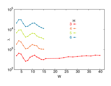
Figure 4: (Color online.) Convergence of the PCC decay length $\lambda$ with slab width $W$. Curves at four slab heights $H=3,4,5,6$ are equally spaced, showing that the linear coefficient of $\ln\lambda$’s dependence on $H$ is independent of $W$.

Figure 5: (Color online.) Scattering length at disorder strength $U=2$. We show $G(L=2)/G(L)$ as a function of wire length $L$ in a $10\times 10$ wire. The dotted line shows a best linear fit. Its slope, $0.031$, is the inverse scattering length $\lambda^{-1}$. $E_{F}=0.7$ in both the sample and the leads, and the disorder strength is $U=2$. The number of samples is $N=864$.

Figure 5 supports our measurement of the scattering length $\lambda\approx 30$, which we obtain by fitting the conductance to $\frac{G(L=0)}{G(L)}=(L/\lambda)+\rho$, where $\rho$ includes the physics of the contact resistance. Beenakker (1997) We use $G(L=2)$ instead of $G(L=0)$, which causes only a small error in our fitting. The scattering length is determined to be $\lambda=(0.031)^{-1}$.

Appendix C Large Slabs and Wires Give Identical Results in the Diffusive Regime

In the main article we state that in the diffusive regime both large slabs and wires have the same conductivity. Here in Figure 5 we plot raw $\sigma$ data for both types of samples, as a function of finite wire circumference and finite wire width. We set the disorder strength $U=7.2$ in the resonance, and the sample height is $H=6$ for both wires and slabs. We set the Fermi energy $E_{F}=0.0$ in the sample and $E_{F}=2.0$ in the leads, but identical results are obtained when $E_{F}=0.2$ in the sample. The number of statistics is $N=12000$ at $W=5,10$, $N=9600$ at $W=15$, $N=4800$ at $W=20$, $N=2400$ at $W=30$, $N=960$ at $W=40$, and $N=480$ at $W\geq 50$.

The main result of these figures is that the conductance $\sigma$ converges quickly with sample width/circumference, and that at $W>40$ there is little or no difference between slabs and wires. In particular, the Berry phase gap has little effect at $W>40$ for two reasons: (1) The gap size scales with $1/W$, and (2) the sample is in diffusive regime, where the disorder broadens the band edges and erases the gap.

Figure 6: (Color online.) Large diffusive slabs and wires give identical conductivities. (a) Convergence with wire circumference $2(W+H)$ of $\sigma$ in wires. (b) Convergence with slab width $W$ of $\sigma$ in slabs with lengths $L=25,\,33,\,50,\,100$. The disorder strength is in the resonance $U=7.2$ and the Fermi energy energy is $E_{F}=0$. Identical results are found at $E_{F}=0.2$.

Appendix D Disorder-Assisted Tunneling Between the Leads in Very Short Slabs

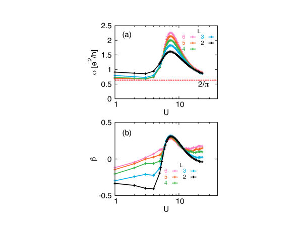
Figure 7: (Color online.) Disorder-assisted tunneling in very short TI slabs. We plot $\sigma(L)$ and its derivative $\beta(L)$ as functions of disorder strength $U$ in slabs with very short lengths $L=2,3,4,5,6$.

In the main article we briefly discuss disorder-assisted tunneling between the leads, which in short samples increases the conductivity and reverses the sign of the beta function and its derivative. Here in Figure 7 we highlight disorder-assisted tunneling between the leads, which occurs in very short samples. This is raw data obtained by averaging $N=4320$ samples. We use slabs with a $6\times 60$ cross-section, and set the Fermi energy at $E=0$ in the sample and $E=2$ in the leads.

The surface states’ resonance with the bulk band is visible as a peak in both $\sigma$ and $\beta$. Inside this peak the derivative $\beta(L)$ is a positive and slowly decreasing function of $L$, as expected from scaling theory. On the wings of the resonance $\beta$ is a negative and increasing function of $L$, because tunneling between the leads increases the conductance. This tunneling has the greatest effect at $L=2$, and decays rapidly with sample length, causing the decreasing conductivity and negative beta.

This data should be compared to wide $W\gg L$ graphene strips, where at small $L$ the conductivity converges to $\frac{4}{\pi}\frac{e^{2}}{h}$, and at other $L$ the conductivity is always greater than $\frac{4}{\pi}\frac{e^{2}}{h}$. Mucciolo and Lewenkopf (2010) Moreover at small $L$ graphene’s $\beta$ converges to zero. Like graphene, our data does show that in TIs at the Dirac point the conductivity is never smaller than $\frac{2}{\pi}\frac{e^{2}}{h}$. (The factor of $2$ difference is associated with the different number of Dirac cones in TIs.) However, unlike graphene our data also shows that in TIs the conductivity at $L\rightarrow 0$ depends on disorder and is always larger than $\frac{2}{\pi}\frac{e^{2}}{h}$, presumably because disorder increases the coupling between the leads. This is manifested also in the $L\rightarrow 0$ limit of $\beta$, which is nonzero and depends on disorder.

Appendix E Convergence of the Conductivity and the $\beta$ Function with Slab Height and Width

Figure 8: (Color online.) Finite size effects on the conductivity $\sigma$ and on the $\beta$ function. (a) Corrections to the conductivity caused by the slab height $H$. We compare $H=6$ to $H=12$ and keep the width fixed at $W=40$. (c) Corrections to $\beta$ caused by the slab height $H=6,12$, with $W=40$. (b) Corrections to the conductivity caused by slab width $W$. We compare $W=40$ to $W=80$ and keep the height fixed at $H=6$. (d) Corrections to $\beta$ caused by slab width $W=40,80$ with $H=6$. We used $N=4800$ samples for the $H=12,W=40$ data, $N=8640$ samples for the the $H=6,W=40$ data, and $N=2160$ samples for the $H=6,W=80$ data.

Here in Figure 8 we examine finite size corrections to the $\sigma$ and $\beta$ curves in panes b and d of the main article’s Figure 8. We use the same parameters as in the main article’s Figure 3. The only difference is that in panes a and c of Figure 8 we change the slab height from $H=12$ to $H=6$, and then plot the ratios of $\sigma$’s and $\beta$’s values at these heights. Similarly in panes b and d of Figure 8 we change the slab width from $W=40$ to $W=80$ while keeping the slab height fixed at $H=6$, and then plot the ratios of $\sigma$’s and $\beta$’s values at these two widths $W=40,80$. In order to reduce noise in $\beta$ we have splined and smoothed the conductivity data prior to computing $\beta$.

Panes a and c of Figure 8 compare the slab heights $H=6,12$. We expect that $H=12$ is quite close to the $H=\infty$ limit because height effects should be regulated by an exponential. At $L>7$ the main effect of tunneling in thin slabs is to multiply the conductivity by a factor which is less than one. Figure 8a show that this factor is very weakly dependent of length $L>7$, and is roughly independent of the Fermi energy $E$. However the tunneling factor does depend on the disorder strength $U$ - it is a 10% effect at the resonance center $U=7.2$, and a 13-14% effect at other disorder strengths. Because the tunneling factor depends only weakly on length $L>7$, the tunneling effect on $\beta$ is rather small, as seen in pane (c). Since the $H=6$ tunneling errors in both $\beta$ and $\sigma$ are small, we expect that tunneling errors are negligible in the $H=12$ data presented in the main article’s Figure 3.

Panes b and d of Figure 8 compare the slab widths $W=40,80$. This error should be regulated by $1/W$, so the difference between $W=80$ and $W=\infty$ will be of the same magnitude as the difference plotted here between $W=40$ and $W=80$. Pane (b) shows that in smaller slabs the conductivity is overestimated by a few percent. We have considered correcting the $W=40$ data in the main article’s Figure 8 to account for the overestimate of $\sigma$, but the correction makes little visible impact on Figure 8 and no change in our conclusions. Pane (d) shows that in $W=40$ slabs at $L>7$ the finite size error in the $\beta$ function is small enough that it is difficult to distinguish from statistical noise, and depends in a complicated way on the Fermi level, the disorder strength, and the sample length. $\beta$ may be either overestimated or underestimated by as much as 7%, but usually around 3-4%, close to the noise level. Both the complicated profile and the small magnitude of the finite size error in $\beta$ imply that this error does not affect our conclusions.

Appendix F Convergence of the Conductance with Height and Width in Slabs and Wires

Figure 9: (Color online.) Convergence of the conductance $G$ as a function of cross-section in short wires and slabs. (a) The conductance as a function of slab length $L$, at many slab heights $H$. The inset magnifies the $L=[100,800]$ data. The slab width is $W=20$. Panes (b-d) show the conductance at disorder $U=2$, divided by its quantized value in pure samples where the conductance is independent of $L$. (c) Convergence with slab width $W$, with a closeup shown in the inset. (b) Convergence with $W=H$ in square wires. (d) Convergence with width $W$ in rectangular wires of height $H=16$, with a closeup shown in the inset.

Panes 3b,3c, and 3d of the main article’s Figure 3 plot the conductivity and beta function in slabs of width $W=44$ and height $H=12$. Here in Figure 9 we examine conductance’s convergence as a function of cross-section in both slabs and wires.

In pane 9a we keep the slab width fixed at $W=20$, so that the conductance should converge to a height-independent value. In panes 9b-9d we obtain a convergent observable by dividing the conductance at disorder strength $U=2$ by its value in a pure sample where the conductance is independent of length. In all panes the disorder strength is $U=2$, and the Fermi energy is $E_{F}=0.7$ both in the leads and in the sample. The number of samples is $N=240$ in panes 9a, 9c, and 9d. In Pane 9b we calculated $9600$ wires with $2\times 2$ and $3\times 3$ cross-sections, $4800$ wires with a $4\times 4$ cross-section, $480$ wires with $6\times 6$ and $8\times 8$ cross-sections, $120$ wires with $10\times 10$ and $20\times 20$ cross-sections, and finally $60$ wires with a $35\times 35$ cross-section.

Pane 9a shows that in slabs $H=3$ is sufficient to obtain good convergence at $L<100$ and that $H=6$ gives good convergence out to $L=800$. Pane 9c shows that in $H=16$ slabs fairly good convergence is obtained at $W=20$ but $W=40$ gives even better results. Interestingly, $W=15$ gives poorer results than $W=10$. The delayed convergence at $L\geq 80$ is caused by the PCCs which cause $G(U=2)/G(L=0)$ to scale with $1/W$. Pane 9b shows that in $W\times W$ wires $W=6$ already gives good convergence at $L<300$. Pane 9d shows that in $W\times 16$ wires fairly good convergence is obtained at $W=4,8,10$, but the best convergence is found when $W>40$.

From Figure 9a, in conjunction with Figure 4 in the supporting material, we conclude that the surface states’ penetration depth is very short, and that convergence with respect to slab height is controlled by an exponential. As long as $L<100$ we can expect very thin $H=3,4$ slabs to give nearly converged results. These results were obtained at disorder strength $U=2$, and we can expect some change at larger disorders $U=8,40$. However since we are using surface disorder we expect the convergence threshold in slabs to shift by only $2$, to $H=5,6$. The small-$W$ data in figures 9b and 9d show the same very fast decay of tunneling in thin wires.

Figures 9b and 9d also show that convergence is not fully achieved until dimensions of $30-60$ are reached. This is not a tunneling effect, but instead a finite size effect caused by the finite lateral dimension in slabs, and by the finite circumference in wires. It is small compared to the tunneling effect, but persists to much larger cross-sections.

In conclusion, the results of Figure 9 inform us that in the main article’s Figure 3 tunneling effects should be small because the height is $H=12$, and finite size effects should also be small because the width is $W=44$.

Appendix G Agreement of $\beta$’s First Derivative with Scaling Theory

Figure 10: (Color online.) $\beta$’s first derivative. $\frac{d\beta(L)}{d\ln L}$ (solid lines) vs. the scaling theory prediction $-\beta^{2}$ (dashed lines) at $L=26$ and four Fermi levels.

In the main article’s Figure 3c we checked the agreement of $\beta$ with the scaling theory prediction $2/\pi\sigma$, as a function of disorder strength $U$ and at four Fermi levels. Here in Figure 10 we examine $\beta$’s first derivative $\frac{d\beta(L)}{d\ln L}$, which should be equal to $-\beta^{2}$ if scaling theory holds. Both $\beta$ and its first derivative were calculated at $L=26$ after doing a linear fit to our raw $\beta$ data over the range $\ln L=[\ln 5,\ln 54]$. We used $N=480$ $6\times 60\times 60$ slabs for this calculation. Our results show that in the resonance center the scaling theory prediction is roughly verified, but outside of the center the agreement vanishes. The main article’s Figure 3d shows that when we increase the slab size and the length $L$ the disagreement seen here is considerably diminished at large $L$, hinting that $\frac{d\beta(L)}{d\ln L}$’s agreement with $-\beta^{2}$ also may improve at large $L$.

References

- Kane and Mele (2005) C. L. Kane and E. J. Mele, Physical Review Letters 95, 226801 (2005).
- Min et al. (2006) H. Min, J. E. Hill, N. A. Sinitsyn, B. R. Sahu, L. Kleinman, and A. H. MacDonald, Physical Review B 74, 165310 (2006).
- Zhang et al. (2009) H. Zhang, C.-X. Liu, X.-L. Qi, X. Dai, Z. Fang, and S.-C. Zhang, Nature Physics 5, 438 (2009).
- Hasan and Kane (2010) M. Z. Hasan and C. L. Kane, Reviews of Modern Physics 82, 3045 (2010).
- Li et al. (2012) Y. Q. Li, K. H. Wu, J. R. Shi, and X. C. Xie, Front. Phys. 7, 165 (2012).
- Culcer (2012) D. Culcer, Physica E 44, 860 (2012).
- Bardarson and Moore (2013) J. H. Bardarson and J. E. Moore, Reports on Progress in Phyiscs 76, 056501 (2013).
- Hsieh et al. (2008) D. Hsieh, D. Qian, L. Wray, Y. Xia, Y. S. Hor, R. J. Cava, and M. Z. Hasan, Nature 452, 970 (2008).
- Hanaguri et al. (2010) T. Hanaguri, K. Igarashi, M. Kawamura, H. Takagi, and T. Sasagawa, Physical Review B 82, 081305(R) (2010).
- Zirnbauer (1992) M. R. Zirnbauer, Physical Review Letters 69, 1584 (1992).
- Mirlin et al. (1994) A. D. Mirlin, A. Muller-Groeling, and M. R. Zirnbauer, Ann. Phys. 236, 325 (1994).
- Ando and Suzuura (2002) T. Ando and H. Suzuura, J. Phys. Soc. Jpn. 71, 2753 (2002).
- Takane (2004) Y. Takane, J. Phys. Soc. Jpn. 73, 1430 (2004).
- Ryu et al. (2007) S. Ryu, C. Mudry, H. Obuse, and A. Furusaki, Physical Review Letters 99, 116601 (2007).
- Ostrovsky et al. (2010) P. M. Ostrovsky, I. V. Gornyi, and A. D. Mirlin, Physical Review Letters 105, 036803 (2010).
- Zhang and Vishwanath (2010) Y. Zhang and A. Vishwanath, Physical Review Letters 105, 206601 (2010).
- Hong et al. (2013) S. S. Hong, Y. Zhang, J. J. Cha, X.-L. Qi, and Y. Cui, arXiv.org arXiv:1303.1601v1 (2013).
- Ostrovsky et al. (2007) P. M. Ostrovsky, I. V. Gornyi, and A. D. Mirlin, Physical Review Letters 98, 256801 (2007).
- Nomura et al. (2007) K. Nomura, M. Koshino, and S. Ryu, Physical Review Letters 99, 146806 (2007).
- Bardarson et al. (2007) J. H. Bardarson, J. Tworzydlo, P. W. Brouwer, and C. W. J. Beenakker, Physical Review Letters 99, 106801 (2007).
- San-Jose et al. (2007) P. San-Jose, E. Prada, and D. S. Golubev, Physical Review B 76, 195445 (2007).
- Tworzydlo et al. (2008) J. Tworzydlo, C. W. Groth, and C. W. J. Beenakker, Physical Review B 78, 235438 (2008).
- Lewenkopf et al. (2008) C. H. Lewenkopf, E. R. Mucciolo, and A. H. CastroNeto, Physical Review B 77, 081410(R) (2008).
- Adam et al. (2009) S. Adam, P. W. Brouwer, and S. DasSarma, Phys. Rev. B 79, 201404(R) (2009).
- Mucciolo and Lewenkopf (2010) E. R. Mucciolo and C. H. Lewenkopf, J. Phys.: Condens. Matter 22, 273201 (2010).
- Mong et al. (2012) R. S. K. Mong, J. H. Bardarson, and J. E. Moore, Physical Review Letters 108, 076804 (2012).
- Asada et al. (2004) Y. Asada, K. Slevin, and T. Ohtsuki, Physical Review B 70, 035115 (2004).
- Schubert et al. (2012) G. Schubert, H. Fehske, L. Fritz, and M. Vojta, Physical Review B 85, 201105 (2012).
- Caroli et al. (1971) C. Caroli, R. Combescot, P. Nozieres, and D. Saint-James, Journal of Physics C 4, 916 (1971).
- Meir and Wingreen (1992) Y. Meir and N. S. Wingreen, Physical Review Letters 68, 2512 (1992).
- Sancho et al. (1985) M. P. L. Sancho, J. M. L. Sancho, and J. Rubio, Journal of Physics F: Metal Physics 15, 851 (1985).
- Groth et al. (2009) C. W. Groth, M. Wimmer, A. R. Akhmerov, J. Tworzydlo, and C. W. J. Beenakker, Physical Review Letters 103, 196805 (2009).
- Guo et al. (2010) H.-M. Guo, G. Rosenberg, G. Refael, and M. Franz, Physical Review Letters 105, 216601 (2010).
- Chen et al. (2012) L. Chen, Q. Liu, X. Lin, X. Zhang, and X. Jiang, New Journal of Physics 14, 043028 (2012).
- Xu et al. (2012) D. Xu, J. Qi, J. Liu, V. Sacksteder, X. C. Xie, and H. Jiang, Physical Review B 85, 195140 (2012).
- Kobayashi et al. (2014) K. Kobayashi, T. Ohtsuki, K. I. Imura, and I. F. Herbut, Physics Review Letters 112, 016402 (2014).
- Analytis et al. (2010) J. G. Analytis, J.-H. Chu, Y. Chen, F. Corredor, R. D. McDonald, Z. X. Shen, and I. R. Fisher, Physical Review B 81, 205407 (2010).
- Brahlek et al. (2011) M. Brahlek, Y. S. Kim, N. Bansal, E. Edrey, and S. Oh, Applied Physics Letters 99, 012109 (2011).
- ValdesAguilar et al. (2012) R. ValdesAguilar, A. V. Stier, W. Liu, L. S. Bilbro, D. K. George, N. Bansal, L. Wu, J. Cerne, A. G. Markelz, S. Oh, et al., Physical Review Letters 108, 087403 (2012).
- Tereshchenko et al. (2011) O. E. Tereshchenko, K. A. Kokh, V. V. Atuchin, K. N. Romanyuk, S. V. Makarenko, V. A. Golyashov, A. S. Kozhukhov, I. P. Prosvirin, and A. A. Shklyaev, JETP Letters 94, 465 (2011).
- Hsieh et al. (2009) D. Hsieh, Y. Xia, D. Qian, L. Wray, J. H. Dil, F. Meier, J. Osterwalder, L. Patthey, J. G. Checkelsky, N. P. Ong, et al., Nature 460, 1101 (2009).
- Noh et al. (2011) H. J. Noh, J. Jeong, E. J. Cho, H. K. Lee, and H. D. Kim, EPL 96, 47002 (2011).
- Liu et al. (2012) Z. K. Liu, Y. L. Chen, J. G. Analytis, S. K. Mo, D. H. Lu, R. G. Moore, I. R. Fisher, Z. Hussain, and Z. X. Shen, Physica E 44, 891 (2012).
- Lang et al. (2011) M. Lang, L. He, F. Xiu, X. Yu, J. Tang, Y. Wang, X. Kou, W. Jiang, A. V. Fedorov, and K. L. Wang, ACS Nano 6, 295 (2011).
- Chen et al. (2010) J. Chen, H. J. Qin, F. Yang, J. Liu, T. Guan, F. M. Qu, G. H. Zhang, J. R. Shi, X. C. Xie, C. L. Yang, et al., Physical Review Letters 105, 176602 (2010).
- Kong et al. (2011) D. Kong, J. J. Cha, K. Lai, H. Peng, J. G. Analytis, S. Meister, Y. Chen, H.-J. Zhang, I. R. Fisher, Z.-X. Shen, et al., ACS Nano 5, 4698 (2011).
- Wu et al. (2013) Q. Wu, L. Du, and V. E. Sacksteder, Physical Review B 88, 045429 (2013).
- Rosenberg et al. (2010) G. Rosenberg, H.-M. Guo, and M. Franz, Physical Review B 82, 041104 (2010).
- Egger et al. (2010) R. Egger, A. Zazunov, and A. L. Yeyati, Physical Review Letters 105, 136403 (2010).
- Bardarson et al. (2010) J. H. Bardarson, P. W. Brouwer, and J. E. Moore, Physical Review Letters 105, 156803 (2010).
- Ando (2006) T. Ando, Journal of the Physical Society of Japan 75, 054701 (2006).
- Altshuler and Aronov (1981) B. L. Altshuler and A. G. Aronov, JETP Letters 33, 499 (1981).
- Dufouleur et al. (2013) J. Dufouleur, L. Veyrat, A. Teichgraber, S. Neuhaus, C. Nowka, S. Hampel, J. Cayssol, J. Schumann, B. Eichler, O. G. Schmidt, et al., Physical Review Letters 110, 186806 (2013).
- Kawarabayashi and Ohtsuki (1996) T. Kawarabayashi and T. Ohtsuki, Phys. Rev. B 53, 6975 (1996).
- Kawabata (2003) A. Kawabata, in Lect. Notes Phys. (2003), pp. 41–51.
- Asada et al. (2006) Y. Asada, K. Slevin, and T. Ohtsuki, Physica E 34, 228 (2006).
- Markos and Schweitzer (2006) P. Markos and L. Schweitzer, J. Phys. A: Math. Gen 39, 3221 (2006).
- Abrahams et al. (1979) E. Abrahams, P. W. Anderson, D. C. Licciardello, and T. V. Ramakrishnan, Physical Review Letters 42, 673 (1979).
- Hikami et al. (1980) S. Hikami, A. I. Larkin, and Y. Nagaoka, Prog. Theor. Phys. Progress Letters 63, 707 (1980).
- Beenakker (1997) C. W. J. Beenakker, Reviews of Modern Physics 69, 731 (1997).