Functional derivatives applied to error propagation of uncertainties in topography to large-aperture scintillometer-derived heat fluxes

Zusammenfassung

Scintillometer measurements allow for estimations of the refractive index structure parameter $C_{n}^{2}$ over large areas in the atmospheric surface layer. Turbulent fluxes of heat and momentum are inferred through coupled sets of equations derived from the Monin–Obukhov similarity hypothesis. One-dimensional sensitivity functions have been produced that relate the sensitivity of heat fluxes to uncertainties in single values of beam height over flat terrain. However, real field sites include variable topography. We develop here, using functional derivatives, the first analysis of the sensitivity of scintillometer-derived sensible heat fluxes to uncertainties in spatially distributed topographic measurements. Sensitivity is shown to be concentrated in areas near the center of the beam path and where the underlying topography is closest to the beam height. Relative uncertainty contributions to the sensible heat flux from uncertainties in topography can reach 20 % of the heat flux in some cases. Uncertainty may be greatly reduced by focusing accurate topographic measurements in these specific areas. A new two-dimensional variable terrain sensitivity function is developed for quantitative error analysis. This function is compared with the previous one-dimensional sensitivity function for the same measurement strategy over flat terrain. Additionally, a new method of solution to the set of coupled equations is produced that eliminates computational error.

Large-aperture scintillometers infer the index of refraction structure parameter $C_{n}^{2}$ over large areas of terrain in the atmospheric surface layer. The structure parameter for temperature $C_{T}^{2}$ is resolved, and this information solves for the sensible heat flux $H_{\mathrm{S}}$ through the application of equations derived from the Monin–Obukhov similarity hypothesis (Hartogensis et al., 2003; Moene, 2003). The sensible heat flux in the atmospheric surface layer is given by

$$H_{\mathrm{S}}=-\rho c_{p}u_{\star}T_{\star},$$ (1)

where $\rho$ is the density of air, $c_{p}$ is the heat capacity at constant pressure, $u_{\star}$ is the friction velocity, and $T_{\star}$ is the temperature scale (e.g., Monin and Obukhov, 1954; Obukhov, 1971; Sorbjan, 1989; Foken, 2006). The temperature scale $T_{\star}$ is resolved by [left=T_⋆= ]alignat=2 & ±CT2az_eff^1/3(1-bζ)^1/3    ζ≤0 ,
±CT2azeff1/3(1+cζ2/3)1/2    ζ≥0 , where $z_{\text{eff}}$ is the effective beam height above the ground, $\zeta\equiv z_{\text{eff}}/l$, where $l$ is the Obukhov length (e.g., Sorbjan, 1989), and $a$, $b$ and $c$ are empirical parameters. The values of the empirical parameters are taken to be $a=4.9$, $b=6.1$, and $c=2.2$, as seen in Andreas (1989) after an adjustment from the original values seen in Wyngaard et al. (1971). These values may not be appropriate for all field sites. We will assume that $C_{T}^{2}$ is resolved by neglecting the influence of humidity fluctuations, although this does not influence our results.

As can be imagined from Eqs. (Functional derivatives applied to error propagation of uncertainties in topography to large-aperture scintillometer-derived heat fluxes) and (Functional derivatives applied to error propagation of uncertainties in topography to large-aperture scintillometer-derived heat fluxes), it is important to know the height $z$ at which $C_{T}^{2}$ is being sampled; this corresponds to the scintillometer beam height. The beam height usually varies along the beam path. Even if turbulence is being sampled above an extremely flat field, uncertainty in $z$ will still be present. Previous studies such as Andreas (1989) and Hartogensis et al. (2003) have quantified the sensitivity of $H_{\mathrm{S}}$ to uncertainties in $z$ over flat terrain. It is the goal of this study to extend the theoretical uncertainty analysis of Andreas (1989) and Hartogensis et al. (2003) to take into account variable terrain along the path. The value of this is in the ability to evaluate uncertainty estimates for scintillometer measurements over variable terrain, as well as to study the theoretical effect that the underlying terrain has on this uncertainty.

The studies of Andreas (1989) and Hartogensis et al. (2003) assume an independently measured friction velocity $u_{\star}$. With large-aperture scintillometers, $u_{\star}$ may be inferred through the Businger–Dyer relation of wind stress, which is coupled to the Monin–Obukhov equations (e.g., Hartogensis et al., 2003; Solignac et al., 2009). Alternatively, with displaced-beam scintillometers, path-averaged values of the inner-scale length of turbulence $l_{o}$ can be measured (in addition to $C_{n}^{2}$), which are related to the turbulent dissipation rate $\epsilon$, which is in turn related through coupled Monin–Obukhov equations to $u_{\star}$ (e.g., Andreas, 1992). As a first step towards a variable terrain sensitivity analysis for large-aperture scintillometers, we will assume independent $u_{\star}$ measurements such that the Businger–Dyer equation will not be considered. Additionally, in order to take into account thick vegetation, the displacement distance $d$ is often introduced. We will not consider this for the purposes of this study.

We are thus considering a large-aperture scintillometer strategy with independent $u_{\star}$ measurements as in Andreas (1989) and Appendix A of Hartogensis et al. (2003), and we consider the line integral effective beam height formulation from Hartogensis et al. (2003) and Kleissl et al. (2008). The effective height formulation is also discussed in Evans and De Bruin (2011) and in Geli et al. (2012). The assumptions behind this line integral approach are that the profile of $C_{T}^{2}$ above the ground satisfies the Monin–Obukhov profile at any point along the beam path, and also that $H_{\mathrm{S}}$ is constant vertically and horizontally within the surface layer region sampled by the beam. In this case, two coupled effects must be taken into account. Firstly, the scintillometer is most sensitive to fluctuations in the index of refraction towards the center of its beam. This is due to the optical configuration of the scintillometer system; a unit-less optical path weighting function takes this into account (e.g., Ochs and Wang, 1974; Hartogensis et al., 2003). The second effect is that, in areas where the topography approaches the beam, the $C_{T}^{2}$ being sampled is theoretically more intense than in areas where the terrain dips farther below the beam.

In Sect. 2 of this paper, we define the sensitivity function $S_{H_{\mathrm{S}},z}(u)$ for the sensible heat flux $H_{\mathrm{S}}$ as a function of variable topography $z(u)$, where $u$ is the relative path position along the beam. In Sect. 3, we solve for $S_{H_{\mathrm{S}},z}(u)$ for any general given $z(u)$. In Sect. 4 we visualize the results by applying the resulting sensitivity function to the topography of a real field site in the North Slope of Alaska. We then apply the resulting sensitivity function to examples of synthetic beam paths. In Sect. 5 we discuss our results, and we conclude in Sect. 6.

1 Definition of the sensitivity function $S_{H_{\mathrm{S}},z}(u)$

Under stable conditions ($\zeta>0$), the set of equations to consider consists of Eqs. (1) and (Functional derivatives applied to error propagation of uncertainties in topography to large-aperture scintillometer-derived heat fluxes), as well as

$$\zeta=\frac{\kappa gT_{\star}z_{\text{eff}}}{{u_{\star}}^{2}T},$$ (2)

$$z_{\text{eff}}=\left(\int_{0}^{1}{{z(u)}^{-2/3}G(u)\mathrm{d}u}\right)^{-3/2},$$ (3)

where $z_{\text{eff}}$ is derived in Kleissl et al. (2008) based on the theory from Hartogensis et al. (2003), $z(u)$ is the height of the beam along the relative path position $u$, $T$ is the temperature, $G(u)$ is the optical path weighting function, $g$ is gravitational acceleration, and $\kappa$ is the von Kármán constant ($0.4$).

For unstable conditions ($\zeta<0$), Eqs. (1), (Functional derivatives applied to error propagation of uncertainties in topography to large-aperture scintillometer-derived heat fluxes) and (2) are considered, but Eq. (3) is replaced by

(4)

where $z_{\text{eff}}$ is derived in Hartogensis et al. (2003).

The propagation of uncertainty from measurements such as $z(u)$ to derived variables such as $H_{\mathrm{S}}$ will be evaluated in the context of the inherent assumptions behind the theoretical equations. A standard approximation (e.g., Taylor, 1997) to the uncertainty in estimating the derived variable $f=f(\mu)$, $\mu=(\mu_{1},\mu_{2},\ldots,\mu_{N})$, by $\hat{f}=f(x)$, a function of measurement variables $x=(x_{1},x_{2},\ldots,x_{N})$, is

$${\sigma^{2}_{f}}= E\big{\{}[f(x)-f(\mu)]^{2}\big{\}}\approx\sum_{i=1}^{N}\left({\frac{\partial f}{\partial x_{i}}}\right)^{2}E\big{[}(x_{i}-\mu_{i}^{2})\big{]}$$

$$=\sum_{i=1}^{N}\left({\frac{\partial f}{\partial x_{i}}}\right)^{2}\sigma_{i}^{2}.$$ (5)

The numerical indices indicate different independent (measurement) variables, such as $T$, $P$, $C_{n}^{2}$, $u_{\star}$, and beam wavelengths $\lambda$ and $z$. It is convenient to re-write Eq. (1) as

$$\left(\frac{{\sigma_{f}}}{f}\right)^{2}=\sum_{i=1}^{N}S_{{f,x_{i}}}^{2}\frac{\sigma_{i}^{2}}{x_{i}^{2}},$$ (6)

where the sensitivity functions $S_{f,x}=$ $(S_{{f,x_{1}}},S_{{f,x_{2}}},\ldots,S_{{f,x_{N}}})$ are defined as

$$S_{{f,x_{i}}}\equiv\frac{x_{i}}{f}\left(\frac{\partial f}{\partial x_{i}}\right).$$ (7)

Sensitivity functions such as these are developed in Andreas (1989) and Andreas (1992). They are each a measure of the portion of relative error in a derived variable $f$ resulting from a relative error in the individual measurement variable $x_{i}$. The problem of resolving the uncertainty in the derived variables is a matter of identifying the magnitude and character of the measurement uncertainties, and then solving for the partial derivative terms in Eqs. (1) and (7).

Here we seek a solution to the sensitivity function of sensible heat flux as a function of topography $S_{H_{\mathrm{S}},z}$. In the flat terrain case, the sensitivity function $S_{H_{\mathrm{S}},z}$ has a single component, corresponding to the single measurement variable $z$ (Andreas, 1989). In our situation, however, we may imagine that since $z(u)$ is distributed over one dimension instead of a single value of $z$, $S_{H_{\mathrm{S}},z}$ will be composed of a spectrum of components:

$$S_{H_{\mathrm{S}},z}=\{S_{H_{\mathrm{S}},z}(u),\ 0\leq u\leq 1\}.$$ (8)

We are thus aiming to expand the sensitivity function denoted “$S_{z}$” in Fig. 4 of Andreas (1989) (our $S_{H_{\mathrm{S}},z}$ in Fig. 8) from one dimension to infinitely many, owing to the fact that some derived variables such as $z_{\text{eff}}$ are functions of an integral over continuous variables $z(u)$ and $G(u)$ (we consider for generality that $z(u)$ has a continuous uncertainty $\sigma(u)^{2}$). In other words, $z_{\textrm{eff}}=z_{\textrm{eff}}[z]$ is a functional, having argument $z=\{z(u),\ 0\leq u\leq 1\}$.

Being dependent on a continuum of measurement variables, the sensitivity function $S_{H_{\mathrm{S}},z}(u)$ here requires the calculation of a so-called functional derivative, $\delta z_{\textrm{eff}}/\delta z(u)$ (e.g., Courant, 1953; Greiner and Reinhardt, 1996). Functional derivatives have a long history of application to statistical error analysis (e.g., Fernholz, 1983; Beutner, 2010, and many references therein).

For our purposes, a heuristic derivation of $\delta z_{\textrm{eff}}/\delta z(u)$ results from an interpretation of the integral in $z_{\textrm{eff}}$ as the limit of Riemann sums. That is,

$$z_{\text{eff}}= \left(\int\limits_{0}^{1}{{z(u)}^{-2/3}G(u)\mathrm{d}u}\right)^{-3/2}\equiv$$

$$\left(\lim_{N\to\infty}\sum\limits_{i=1}^{N}{z_{i}}^{-2/3}G_{i}\cdot(1/N)\right)^{-3/2},$$ (9)

where subscript $i$ indicates that $u=(i/N)$. Upon discretizing the input variables, we have

$$\left(\frac{\partial z_{\text{eff}}}{\partial z_{k}}\right) =$$

$$-\frac{3}{2}\left(\sum\limits_{i=1}^{N}{z_{i}}^{-2/3}G_{i}\cdot(1/N)\right)^{-5/2}$$

$$\frac{\partial}{\partial z_{k}}\left(\sum\limits_{i=1}^{N}{z_{i}}^{-2/3}G_{i}\cdot(1/N)\right)$$

$$=-\frac{3}{2}\left(\sum\limits_{i=1}^{N}{z_{i}}^{-2/3}G_{i}\cdot(1/N)\right)^{-5/2}$$

$$\quad\times-\frac{2}{3}\left({z_{k}}^{-5/3}G_{k}\cdot(1/N)\right)$$

$$=\left(\sum\limits_{i=1}^{N}{z_{i}}^{-2/3}G_{i}\cdot(1/N)\right)^{-5/2}$$

$${z_{k}}^{-5/3}G_{k}\cdot(1/N).$$ (10)

Letting $k=\arg\,\min_{k}|z(u)-z_{k}|$ and taking the limit $N\to\infty$, the desired functional derivative is given by

$$\left(\frac{\delta z_{\text{eff}}}{\delta z(u)}\right) =\left(\int\limits_{0}^{1}{{z(u)}^{-2/3}G(u)\mathrm{d}u}\right)^{-5/2}{z(u)}^{-5/3}G(u).$$ (11)

We thus define

$$S_{H_{\mathrm{S}},z}(u)\equiv\frac{z(u)}{H_{\mathrm{S}}[z]}\left(\frac{\delta H_{\mathrm{S}}}{\delta z(u)}\right)$$ (12)

as the sensitivity function of sensible heat flux $H_{\mathrm{S}}$ to uncertainties in variable topography $z(u)$. It is our goal to evaluate Eq. (12).

2 Solution of the sensitivity function $S_{H_{\mathrm{S}},z}(u)$

2.1 Stable conditions ($\zeta>0$)

Under stable conditions, the set of Eqs. (1), (Functional derivatives applied to error propagation of uncertainties in topography to large-aperture scintillometer-derived heat fluxes), (2) and (3) is coupled in $l$ through $\zeta$; we begin de-coupling them by combining Eqs. (Functional derivatives applied to error propagation of uncertainties in topography to large-aperture scintillometer-derived heat fluxes) and (2) to obtain

$$\zeta=(\pm)\frac{\kappa g{z_{\text{eff}}}^{4/3}\sqrt{{C^{2}_{T}}}}{{u_{\star}}^{2}T\sqrt{a}(1+c\zeta^{2/3})^{1/2}}.$$ (13)

Since $\zeta>0$, the unsolved sign is positive. With the substitution

$$\hat{\Lambda}\equiv\frac{\kappa^{2}g^{2}{C^{2}_{T}}}{{u_{\star}}^{4}T^{2}a},$$ (14)

we re-arrange Eq. (13) to obtain

$$\zeta^{2}+c\zeta^{8/3}-{\hat{\Lambda}}{z_{\text{eff}}}^{8/3}=0,$$ (15)

where $z_{\text{eff}}$ in the stable case is determined by a priori known functions $z(u)$ and $G(u)$ through Eq. (3). The value of $\hat{\Lambda}$, including $C_{T}^{2}$, is directly determined from the measurements. The solution of Eq. (15) follows by re-writing it as a fourth-degree algebraic equation in $\zeta^{2/3}$:

$$(\zeta^{2/3})^{3}+c(\zeta^{2/3})^{4}-{\hat{\Lambda}}{z_{\text{eff}}}^{8/3}=0,$$ (16)

or more practically, it can be solved through fixed-point recursion on the function

$$\zeta=\sqrt{\frac{{\hat{\Lambda}}z_{\text{eff}}^{8/3}}{1+c\zeta^{2/3}}}\equiv\hat{F}(\zeta),$$ (17)

where we must consider the positive root. Note that since Eq. (16) is fourth degree, Galois theory states that it has an explicit solution form (e.g., Edwards, 1984). It is thus possible in theory to write $H_{\mathrm{S}}=h(z(u),C_{n}^{2},P,T,\lambda,u_{\star})$, where $h$ is an explicit function of the measurements; however, it would be quite an unwieldy equation.

We do not need an explicit solution in order to study the sensitivity; we can use the chain rule and implicit differentiation as in Gruber and Fochesatto (2013). We establish the variable inter-dependency using Eq. (15) as a starting point. The tree diagram for any set of measurements under stable conditions is seen in Fig. 1. The measurements are at the ends of each branch, and all other variables are dependent.

The required global partial derivatives are now defined through the variable definitions, the above equations, and the tree diagram. We have

$$\left(\frac{\delta H_{\mathrm{S}}}{\delta z(u)}\right)= \left(\frac{\partial H_{\mathrm{S}}}{\partial T_{\star}}\right)\left(\left(\frac{\partial T_{\star}}{\partial z_{\text{eff}}}\right)_{\zeta}\right.$$

$$\left.+\left(\frac{\partial T_{\star}}{\partial\zeta}\right)\left(\frac{\partial\zeta}{\partial z_{\text{eff}}}\right)\right)\left(\frac{\delta z_{\text{eff}}}{\delta z(u)}\right).$$ (18)

We will need one derivative that we are not able to retrieve directly from explicit definitions. By implicitly differentiating Eq. (15) under the guidance of the tree diagram seen in Fig. 1, we derive

$$\left(\frac{\partial\zeta}{\partial z_{\text{eff}}}\right)=\left(\frac{4{\hat{\Lambda}}{z_{\text{eff}}}^{5/3}}{3\zeta+4c\zeta^{5/3}}\right)=\frac{1}{z_{\text{eff}}}\left(\frac{4\zeta(1+c\zeta^{2/3})}{3+4c\zeta^{2/3}}\right).$$ (19)

The functional derivative term $\left(\frac{\delta z_{\text{eff}}}{\delta z(u)}\right)$ for stable conditions has been evaluated in Eq. (11).

2.2 Unstable conditions ($\zeta<0$)

Under unstable conditions, the set of Eqs. (1), (Functional derivatives applied to error propagation of uncertainties in topography to large-aperture scintillometer-derived heat fluxes), (2) and (LABEL:zeffunstable) is coupled in $l$ through $\zeta$; note that $z_{\text{eff}}$ is coupled to $\zeta$ in the unstable case. We combine Eqs. (Functional derivatives applied to error propagation of uncertainties in topography to large-aperture scintillometer-derived heat fluxes) and (2) to obtain

$$\zeta=(\pm)\frac{\kappa g\sqrt{{C^{2}_{T}}}}{{u_{\star}}^{2}T\sqrt{a}}{z_{\text{eff}}}^{4/3}(1-b\zeta)^{1/3}.$$ (20)

Since $\zeta<0$, the sign is negative. With the substitution $\breve{\Lambda}\equiv\left(\frac{\kappa g\sqrt{{C^{2}_{T}}}}{{u_{\star}}^{2}T\sqrt{a}}\right)^{3/4}$, this leads to

$$z_{\text{eff}}=\frac{1}{{\breve{\Lambda}}}\frac{(-\zeta)^{3/4}}{(1-b\zeta)^{1/4}}\rightarrow\frac{\zeta}{z_{\text{eff}}}=-{\breve{\Lambda}}(b\zeta^{2}-\zeta)^{1/4}.$$ (21)

We substitute Eq. (21) into Eq. (LABEL:zeffunstable) to obtain

(24)

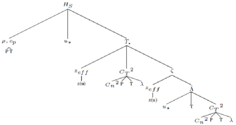
Abbildung 1: Variable inter-dependency tree diagram for the stable case ($\zeta>0$). The measurement variables are at the end of each branch; all other variables are derived.

This single equation is in the single unknown $\zeta$, since $z(u)$, $G(u)$ and ${\breve{\Lambda}}$ are known; it is also in the fixed-point form $\zeta=\breve{F}(\zeta)$. The tree diagram for the unstable case is seen in Fig. 2. Evaluation of global partial derivatives proceeds analogously to the stable case as in Eq. (18). Now we have

$$\left(\frac{\delta H_{\mathrm{S}}}{\delta z(u)}\right)= \left(\frac{\partial H_{\mathrm{S}}}{\partial T_{\star}}\right)\left(\left(\frac{\partial T_{\star}}{\partial z_{\text{eff}}}\right)\left(\frac{\partial z_{\text{eff}}}{\partial\zeta}\right)\right.$$

$$\left.+\left(\frac{\partial T_{\star}}{\partial\zeta}\right)_{z_{\text{eff}}}\right)\left(\frac{\delta\zeta}{\delta z(u)}\right).$$ (25)

To pursue the solution of $S_{H_{\mathrm{S}},z}(u)$, we will need to solve for $\left(\frac{\partial z_{\text{eff}}}{\partial\zeta}\right)$ by the differentiation of Eq. (21):

$$\left(\frac{\partial z_{\text{eff}}}{\partial\zeta}\right)=\frac{(2b\zeta-3)}{4{\breve{\Lambda}}(-\zeta)^{1/4}(1-b\zeta)^{5/4}}=\frac{z_{\text{eff}}(3-2b\zeta)}{4\zeta(1-b\zeta)}.$$ (26)

We can solve for $\left(\frac{\delta\zeta}{\delta z(u)}\right)$ by implicit differentiation of Eq. (LABEL:zetaunstable). In finding $\left(\frac{\delta\zeta}{\delta z(u)}\right)$, it is useful to define

(27)

where, from Eqs. (LABEL:zetaunstable) and (LABEL:fdef), we have

$$\sqrt{f}=(1-2b\zeta).$$ (28)

From Eq. (LABEL:fdef), we have

$$\left(\frac{\delta f}{\delta z(u)}\right)=\left(\frac{\partial f}{\partial\zeta}\right)\left(\frac{\delta\zeta}{\delta z(u)}\right)+\left(\frac{\delta f}{\delta z(u)}\right)_{\zeta},$$ (29)

such that, by implicitly differentiating Eq. (28) and then substituting, we derive

(30)

All the information we need to solve for $S_{H_{\mathrm{S}},z}(u)$ is now resolved.

2.3 Full expression for the sensitivity function $S_{H_{\mathrm{S}},z}(u)$

Since we are considering an independent $u_{\star}$ measurement, we have $S_{T_{\star},z}(u)=S_{H_{\mathrm{S}},z}(u)=\frac{z(u)}{T_{\star}}\left(\frac{\delta T_{\star}}{\delta z(u)}\right)$. We obtain

$$S_{T_{\star},z}(u)=$$ (31)

(43)

3 Application of the results for the sensitivity function $S_{H_{\mathrm{S}},z}(u)$

3.1 Imnavait Creek basin field campaign

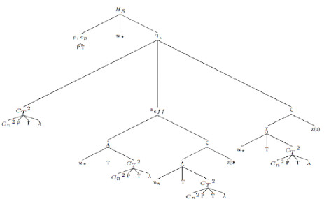
Abbildung 2: Variable inter-dependency tree diagram for the unstable case ($\zeta<0$). The measurement variables are at the end of each branch; all other variables are derived.

As an example, we use topographic data from the Imnavait Creek basin field site (UTM 5N 650220.5 East, 7615761.5 North), where there is a campaign to determine large-scale turbulent fluxes in the Alaskan tundra; it is seen in Figs. 3a and 4. We assume for simplicity that vegetation patterns, water availability, and other changes across the basin that could affect the flow in the atmospheric surface layer do not represent a significant source of surface heterogeneity. The elevation data seen in Fig. 3a are from a $5$ m resolution digital elevation map (DEM), which has a roughly $0.5$ m standard deviation in a histogram of the difference between the DEM elevations and $50$ randomly distributed GPS ground truth points, as seen in Fig. 3b. Note that the systematic offset between the DEM and the GPS ground truth measurements does not contribute to systematic error in $z(u)$. Note also that some of this spread in data may be due to an active permafrost layer.

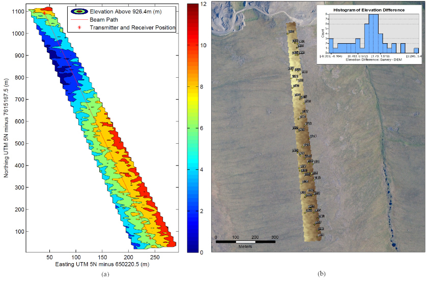
Abbildung 3: Topography and space view of the Imnavait Creek basin, North Slope of Alaska. The scintillometer beam runs roughly north–south on a $1.04$ km path. The emitter and receiver are each raised off the ground by $3.8$ m. Vegetation along the path is representative of Arctic tundra. Superimposed is a histogram of $50$ points of the GPS ground truth elevation survey minus the DEM elevation.

For this field site, we can solve for $\zeta$ under unstable conditions through Eq. (LABEL:zetaunstable). As can be seen in Fig. 5, we arrive at the solution for $\zeta$ with the recursively defined series $[\breve{F}(\zeta_{\text{guess}}),\breve{F}(\breve{F}(\zeta_{\text{guess}})),\breve{F}(\breve{F}(\breve{F}(\zeta_{\text{guess}}))),\dots]$ that is guaranteed to converge monotonically for any $\zeta_{\text{guess}}<0$.

A plot of $\zeta$ as a function of ${\breve{\Lambda}}$ for this field site is seen in Fig. 6. Note that the relationship between $\zeta$ and ${\breve{\Lambda}}$ is bijective; any value of ${\breve{\Lambda}}$ is uniquely associated with a value of $\zeta$.

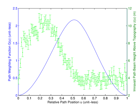
Abbildung 4: Height of the beam above the ground $z$ and the path weighting function $G$ as functions of relative path position $u$, using the Imnavait experimental site as seen in Fig. 3a. Uncertainties are based on the approximate standard deviation in the histogram in Fig. 3b, although they do not influence the analysis presented in this study.

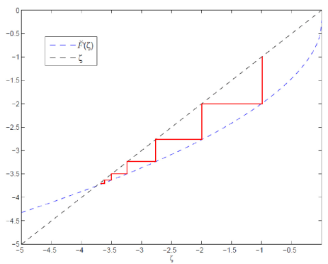
Abbildung 5: Graphical visualization of the fixed-point solution of Eq. (LABEL:zetaunstable). The recursively defined series $[\breve{F}(\zeta_{\text{guess}}),\breve{F}(\breve{F}(\zeta_{\text{guess}})),\breve{F}(\breve{F}(\breve{F}(\zeta_{\text{guess}}))),\dots]$ converges monotonically for any $\zeta_{\text{guess}}<0$. A typical value of ${\breve{\Lambda}}=1/4$ is used, representing slightly unstable conditions in the atmospheric surface layer. The initial guess is $\zeta_{\text{guess}}=-1$, and the path of convergence is shown by the red line. The Imnavait Creek basin terrain and beam path are used for $z(u)$, along with the standard path weighting function $G(u)$ as seen in Figs. 3a and 4.

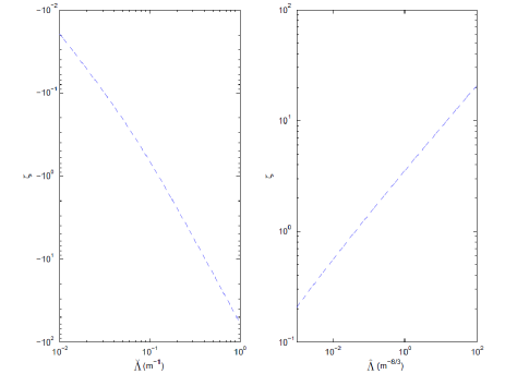
Abbildung 6: Solution of Eqs. (17) and (LABEL:zetaunstable) produced with a monotonically converging series as explained in the text and as visualized in Fig. 5. The Imnavait Creek basin terrain and beam path are used for $z(u)$, along with the standard path weighting function $G(u)$ as seen in Figs. 3a and 4. The mapping between $\zeta$ and $\breve{\Lambda}$ and between $\zeta$ and $\hat{\Lambda}$ is bijective. Note that the solution of $\zeta$ for $\breve{\Lambda}=1/4$ corresponds to the intersection of $\breve{F}$ with $\zeta$ in Fig. 5.

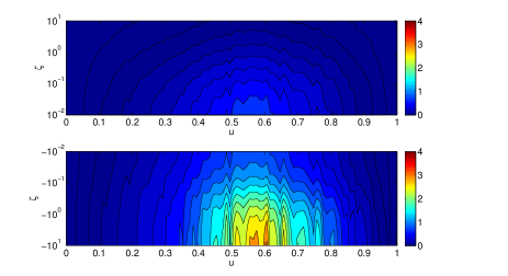
Abbildung 7: Sensitivity function $S_{H_{\mathrm{S}},z}(u)=S_{T_{\star},z}(u)$. For stable conditions ($\zeta>0$), $S_{T_{\star},z}(u)$ is given in Eq. (31). For unstable conditions ($\zeta<0$), $S_{T_{\star},z}(u)$ is given by Eq. (43), where values for $\zeta$ as a function of ${\breve{\Lambda}}$ are obtained through a numerical solution of Eq. (LABEL:zetaunstable), which may be visualized with Fig. 6. The Imnavait Creek basin terrain and beam path are used for $z(u)$, along with the standard path weighting function $G(u)$ as seen in Figs. 3a and 4.

Considering the field case study of the Imnavait Creek basin, where the height of the beam over the terrain $z(u)$ and the standard path weighting function $G(u)$ are seen in Figs. 3a and 4, Eqs. (31) and (43) lead to the sensitivity function seen in Fig. 7. Note that $S_{H_{\mathrm{S}},z}(u)$ is a function of $u$ and $\zeta$ only, since, for any one beam height transect $z(u)$, $\breve{\Lambda}$ is mapped bijectively with respect to $\zeta$ through Eq. (LABEL:zetaunstable), as seen in Fig. 6.

Note that if we consider a constant ratio of $\frac{\sigma_{z}(u)}{z(u)}$, systematic error propagation can be re-written as

$$\int\limits_{0}^{1}{\frac{\sigma_{z}(u)}{z(u)}S_{H_{\mathrm{S}},z}(u)\mathrm{d}u}=\frac{\sigma_{z}(u)}{z(u)}\left[\,\int\limits_{0}^{1}{S_{H_{\mathrm{S}},z}(u)\mathrm{d}u}\right].$$ (44)

The term in square brackets on the right of Eq. (44) is plotted in Fig. 8.

3.2 Synthetic scintillometer beam paths

It is interesting to examine the sensitivity function over synthetic paths that are representative of commonly used paths in scintillometry. Two synthetic paths can be seen in Fig. 9. They include a slant path as well as a quadratic path representing a beam over a valley.

The sensitivity function $S_{T_{\star},z}(u)=S_{H_{\mathrm{S}},z}(u)$ for synthetic path $1$ (the quadratic path) seen in Fig. 9 is seen in Fig. 10. For synthetic path $2$ (the slant path), the sensitivity function is seen in Fig. 11.

4 Discussion

A sensitivity function mapping the propagation of uncertainty from $z(u)$ to $H_{\mathrm{S}}$ has been produced for a large-aperture scintillometer strategy incorporating independent $u_{\star}$ measurements, and the line integral footprint approach to variable topography developed in Hartogensis et al. (2003) and Kleissl et al. (2008). This was accomplished by mapping out the variable inter-dependency as illustrated in the tree diagrams in Figs. 1 and 2, and by applying functional derivatives. The solution to $S_{H_{\mathrm{S}},z}(u)$ is given in Eqs. (12), (31) and (43).

As seen in Figs. 3a, 4, and 7, our results for $S_{T_{\star},z}(u)=S_{H_{\mathrm{S}},z}(u)$ show that sensitivity to uncertainties in topographic heights is generally higher under unstable conditions, and it is both concentrated in the center of the path and in areas where the underlying topography approaches the beam height. This finding intuitively makes sense, since scintillometers are more sensitive to $C_{T}^{2}$ at the center of their beam path, and $C_{T}^{2}$ decreases nonlinearly in height above the surface and strengthens with greater instability. For the Imnavait Creek basin path, the value of $S_{H_{\mathrm{S}},z}(u)$ increases to $3$ at small dips in the beam height beyond the halfway point of the path, as seen in Fig.7. Note that the asymmetry along $u$ of $S_{H_{\mathrm{S}},z}(u)$ corresponds to the asymmetry of the path, which is mostly at a higher ($>$ 6 m) height in the first half, and at a lower height ($\approx$ 4 m) in the second half, as seen in Fig. 4. Also note that the local maxima in $S_{H_{\mathrm{S}},z}(u)$ occur at roughly $u\approx$ 60 % and $u\approx$ 65 %; these correspond directly to topographic protuberances seen in Figs. 3a and 4. Note that the total error in $H_{\mathrm{S}}$ is contributed from the whole range of $u$ along $S_{H_{\mathrm{S}},z}(u)$, so even though we may have values of up to $3$ in the sensitivity functions, our error bars may still be reasonable. The average value of $S_{H_{\mathrm{S}},z}(u)$ along $u$ is never higher than $1$, as seen in Fig. 8. Knowledge of where the concentration in sensitivity is allows us to decrease our uncertainty greatly by taking high-accuracy topographic measurements in these areas, especially for Arctic beam paths, which must be low due to thin boundary layers.

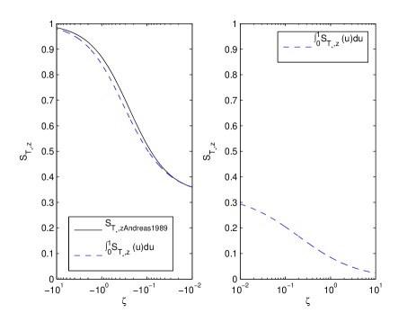
Abbildung 8: Average value of $S_{T_{\star},z}(u)=S_{H_{\mathrm{S}},z}(u)$ over beam path $u$, given by $\int_{0}^{1}{S_{T_{\star},z}(u)\mathrm{d}u}$, and the flat terrain sensitivity function $S_{z}$ derived in Andreas (1989) (for $\zeta>0$, the functions are identical). For stable conditions ($\zeta>0$), $S_{T_{\star},z}(u)$ is given by Eq. (31). For unstable conditions ($\zeta<0$), $S_{T_{\star},z}(u)$ is given by Eq. (43), where values for $\zeta$ as a function of ${\breve{\Lambda}}$ are obtained through a numerical solution of Eq. (LABEL:zetaunstable), which may be visualized in Fig. 6. The Imnavait Creek basin terrain and beam path are used for $z(u)$, along with the standard path weighting function $G(u)$ as seen in Figs. 3a and 4.

For example, if the random error in $z(u)$ in the Imnavait Creek basin were 0.5 m, the relative error resulting in $H_{\mathrm{S}}$ due to uncertainty in $z(u)$ alone would be just 2 % under slightly unstable conditions where $\breve{\Lambda}=1/4$ and $\zeta\approx-3.75$, whereas if we reduce the uncertainty in $z(u)$ to 0.1 m, the relative error in $H_{\mathrm{S}}$ due to uncertainty in $z(u)$ would be just 0.3 %, so with a reasonable number of survey points (100), the error can be quite small. However, if we look at Fig. 3b, we see that there is significant systematic error, perhaps due to shifting permafrost. If we have a perfectly even systematic error across the whole map, then this error is not propagated. However, if we have even a small amount of systematic error such as 0.5 m distributed around the center of the beam path near the local maxima in sensitivity, we can easily achieve 10 % to 20 % relative error in $H_{\mathrm{S}}$. In comparison to other variables, the values for $S_{H_{\mathrm{S}},u_{\star}}$ are similar in magnitude to $S_{H_{\mathrm{S}},z}$ under unstable conditions, smaller under neutral conditions, and larger under stable conditions (Andreas, 1989). Under unstable conditions, error from $u_{\star}$ may therefore be similar in magnitude to error from $z(u)$; however, for path-averaged $u_{\star}$ scintillometer strategies, this is not an issue. For $C_{n}^{2}$, the sensitivity functions are usually smaller, but in isolated regions they are larger (Andreas, 1989).

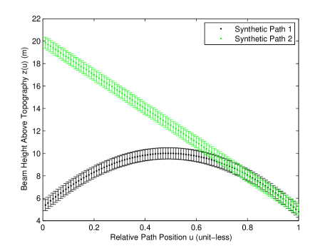
Abbildung 9: Synthetic path beam heights including a quadratic path (path 1) and a slant path (path 2).

The average value of $S_{H_{\mathrm{S}},z}(u)$ over the beam path reduces to identical results to the flat terrain sensitivity function $S_{z}$ from Andreas (1989) (which would be denoted $S_{T_{\star},z}$ here) under stable conditions where $z_{\text{eff}}$ is de-coupled from $\zeta$, and nearly identical results (depending on the path) under unstable conditions where $z_{\text{eff}}$ is coupled to $\zeta$, as seen in Fig. 8. It is unknown as to whether the addition of equations for path-averaged $u_{\star}$ measurements such as the Businger–Dyer relation seen in Hartogensis et al. (2003) and Solignac et al. (2009), or displaced-beam scintillometer strategies as seen in Andreas (1992), would change these results significantly.

We note that the study of Hartogensis et al. (2003) evaluated a function similar to $S_{H_{\mathrm{S}},z}$ for flat terrain with an independent $u_{\star}$ measurement (the 2003 Eq. 7 is ignored); however, at $\zeta\approx 0$ they found a sensitivity of $1/2$ instead of $1/3$ as found in Andreas (1989). The difference in the results between these two studies is not due to the differences between single- and double-wavelength strategies. The Obukhov length (denoted by $L_{\text{MO}}$ in Hartogensis et al., 2003) is a function of $z_{\text{LAS}}$ through the 2003 Eqs. (5) and (6). The addition of chain rule terms to reflect the dependence of $l$ on $z$ in Hartogensis et al.’s (2003) Eq. (A2) resolves differences between Hartogensis et al.’s (2003) Fig. A1 and Andreas et al.’s (1989) Fig. 4; the flat-terrain sensitivity function for $\zeta<0$ is

$$S_{H_{\mathrm{S}},z}=S_{T_{\star},z}=\frac{1-2b\zeta}{3-2b\zeta}\neq\frac{1-2b\zeta}{2-2b\zeta}=\frac{z}{H_{\mathrm{S}}}\left(\frac{\partial H_{\mathrm{S}}}{\partial z}\right)_{l},$$ (45)

which is given correctly in Andreas (1989).

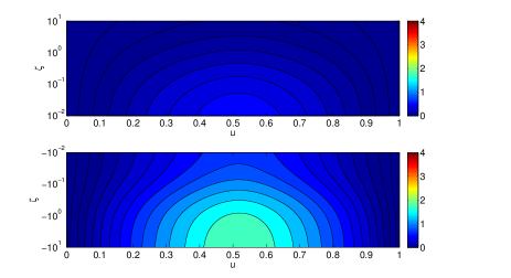
Abbildung 10: Sensitivity function $S_{H_{\mathrm{S}},z}(u)=S_{T_{\star},z}(u)$. For stable conditions ($\zeta>0$), $S_{T_{\star},z}(u)$ is given in Eq. (31). For unstable conditions ($\zeta<0$), $S_{T_{\star},z}(u)$ is given by Eq. (43), where values for $\zeta$ as a function of ${\breve{\Lambda}}$ are obtained through a numerical solution of Eq. (LABEL:zetaunstable), which may be visualized with Fig. 6. Synthetic beam path $1$ (the quadratic path) is used for $z(u)$, along with the standard path weighting function $G(u)$ as seen in Figs. 9 and 4.

Equations (1), (7), (31), and (43) may be implemented into computer code for routine analysis of data. It is worth noting that the sign of $\zeta$ is an a priori unknown from the measurements. Thus, for any set of measurements, we should calculate the set of all derived variables and their respective uncertainties assuming both stable and unstable conditions, and if uncertainties in the range of $\zeta$ overlap with $\zeta=0$ for either stability regime, we should then consider the combined range of errors in the two sets.

In the application of Eq. (1), we must recognize computational error $\sigma_{f_{\mathrm{c}}}$. Previous studies have incorporated a cyclically iterative algorithm that may not converge, as seen in Andreas (2012), or that may converge to an incorrect solution, as illustrated in the section on coupled nonlinear equations in Press et al. (1992). We have developed techniques to eliminate this error. For unstable cases ($\zeta<0$), the solution of $\zeta$ follows from Eq. (LABEL:zetaunstable), which is in fixed-point form. The solution to Eq. (LABEL:zetaunstable) is guaranteed to converge monotonically with the recursively defined series $[\breve{F}(\zeta_{\text{guess}}),\breve{F}(\breve{F}(\zeta_{\text{guess}})),\breve{F}(\breve{F}(\breve{F}(\zeta_{\text{guess}}))),\dots]$ as seen in Traub (1964) and in Agarwal et al. (2001), and as demonstrated in Fig. 5. We may solve for the stable case ($\zeta>0$) recursively using Eq. (17), where $\hat{F}(\zeta)$ demonstrates convergence properties that are similar to those of $\breve{F}(\zeta)$ in Eq. (LABEL:zetaunstable). It was found to be practical to make $\zeta_{\text{guess}}=\pm 1$.

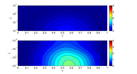
Abbildung 11: Sensitivity function $S_{H_{\mathrm{S}},z}(u)=S_{T_{\star},z}(u)$. For stable conditions ($\zeta>0$), $S_{T_{\star},z}(u)$ is given in Eq. (31). For unstable conditions ($\zeta<0$), $S_{T_{\star},z}(u)$ is given by Eq. (43), where values for $\zeta$ as a function of ${\breve{\Lambda}}$ are obtained through a numerical solution of Eq. (LABEL:zetaunstable), which may be visualized with Fig. 6. Synthetic beam path $2$ (the slant path) is used for $z(u)$, along with the standard path weighting function $G(u)$ as seen in Figs. 9 and 4.

Future expansions of the results presented here should focus on including multiple wavelength strategies to evaluate the latent heat flux and $H_{\mathrm{S}}$, as well as on including path-averaged $u_{\star}$ measurements using $l_{o}$ and $C_{n}^{2}$ scintillometer strategies as in Andreas (1992) or using a point measurement of wind speed and the roughness length via the Businger–Dyer relation (e.g., Panofsky and Dutton, 1984; Solignac et al., 2009). Modification of the analysis for including path-averaged $u_{\star}$ measurements involves the addition of one or two more equations (e.g., Eq. 8 in Solignac et al., 2009, or Eqs. 1.2 and 1.3) in Andreas, 1992) to substitute into Eqs. (15) and (LABEL:zetaunstable), as well as the definition of new tree diagrams to reflect that $u_{\star}$ is now a derived variable. In these cases, either the turbulence inner-scale length $l_{o}$ or a point measurement of wind speed and the roughness length replaces $u_{\star}$ as a measurement; $u_{\star}$ is derived through information from the full set of measurements. Note that if $u_{\star}$ is derived through measurements including $z$, Eq. (1) implies that $S_{H_{\mathrm{S}},z}=S_{T_{\star},z}+S_{u_{\star},z}$. It is worth investigating whether computational error can still be eliminated in these cases.

We have considered here the effective height line integral approach derived in Hartogensis et al. (2003) and Kleissl et al. (2008) to take into account variable topography. Even if we assume a constant flux surface layer, under realistic wind conditions, turbulent air is advected in from nearby topography. For example, in the Imnavait Creek basin path seen in Fig. 3a, if wind comes from the west, the turbulent air being advected into the beam path comes from a volume that is higher above the underlying topography than if wind came from the east. Sensitivity studies should be produced for two-dimensional surface integral methods that take into account the coupling of wind direction and topography on an instrument footprint (e.g., Meijninger et al., 2002; Liu et al., 2011). Additionally, a new theory may be developed for heterogeneous terrain involving complex distributions of water availability and roughness length such as the terrain in the Imnavait Creek basin.

Sensitivity of the sensible heat flux measured by scintillometers has been shown to be highly concentrated in areas near the center of the beam path and in areas of topographic protrusion. The general analytic sensitivity functions that have been evaluated here can be applied for error analysis over any field site as an alternative to complicated numerical methods. Uncertainty can be greatly reduced by focusing accurate topographic measurements in areas of protrusion near the center of the beam path. The magnitude of the uncertainty is such that it may be necessary to use high-precision LIght Detection And Ranging (LIDAR) topographic data as in Geli et al. (2012) for Arctic field sites in order to avoid large errors resulting from uneven permafrost changes since the last available DEM was taken. Additionally, computational error can be eliminated by following a computational procedure as outlined here.