Predicting unobserved exposures from seasonal epidemic data

Abstract

We consider a stochastic Susceptible-Exposed-Infected-Recovered (SEIR) epidemiological model with a contact rate that fluctuates seasonally. Through the use of a nonlinear, stochastic projection, we are able to analytically determine the lower dimensional manifold on which the deterministic and stochastic dynamics correctly interact. Our method produces a low dimensional stochastic model that captures the same timing of disease outbreak and the same amplitude and phase of recurrent behavior seen in the high dimensional model. Given seasonal epidemic data consisting of the number of infectious individuals, our method enables a data-based model prediction of the number of unobserved exposed individuals over very long times.

1 Introduction

As a dynamical process in epidemics, noise increasingly plays an important role when using models to understand and predict disease outbreaks. Stochastic effects figure prominently in finite populations, which can range from ecological dynamics (Marion et al., 2000) to childhood epidemics in cities (Rohani et al., 2002; Nguyen and Rohani, 2008a). For populations with seasonal forcing, noise comes into play in the prediction of large outbreaks (Rand and Wilson, 1991; Billings et al., 2002; Stone et al., 2007). External random perturbations, such as those arising from random migrations (Alonso et al., 2007), change the probabilistic prediction of epidemic outbreak amplitudes as well as their control (Schwartz et al., 2004).

Epidemic stochasticity may arise from several sources, such as internal interactions due to random contacts in finite well-mixed populations (Nåsell, 1999; Doering et al., 2005), as well as contacts on structured contact networks (Shaw and Schwartz, 2008). On the other hand, it may arise from random external fluctuations, such as immigration perturbations (Anderson and May, 1991; Alonso et al., 2007). In many cases, whether noise arises externally or internally, it may have far ranging effects on outbreak predictability. For example, noise impacts predictability in climate and disease (Kelly-Hope and Thomson, 2008), produces random-looking outbreaks from its interaction with mass action terms (Nguyen and Rohani, 2008b), and amplifies the peaks of epidemics due to its interaction with resonant frequencies (Alonso et al., 2007). Other areas of noise research have been postulated as the source of chaos in epidemics (Rand and Wilson, 1991; Billings and Schwartz, 2002), whereby noise explicitly interacts with the underlying topology of the epidemics model. As a direct consequence of its topological interaction, random chaotic-like switching may occur between small amplitude and large outbreaks when including the effects of stochasticity (Billings et al., 2002).

To connect with data, time series analysis from spatio-temporal cases has been done to generate parameters for use in epidemic models. Tools from nonlinear time series analysis of measles data (Schaffer et al., 1993; Blarer and Doebeli, 1999) have pointed to the important realization that any mathematical models might need to capture chaotic behavior, which is deterministic and predictable only in the short term. As a result, time series data analysis has centered on the assumption that a deterministic processes dominates the time series, but quantifying determinism from the statistics may be inconclusive. In Tidd et al. (1993), analysis specifically points out that complex, or chaotic behavior may be detected, even when it is not deterministic. For example, sensitive dependence on initial conditions in short, noisy, non-chaotic time series, such as epidemic data, may be indicated by positive Lyapunov exponents.

Another time series analysis method which also includes noise is that of Time-series Susceptible-Infected-Recovered (TSIR) modeling (Bjornstad et al., 2002). Here the authors do local fits of time-series data from England and Wales to get measures of local reproductive rates of infection. The main assumption is that in the pre-vaccine years, all newborns introduced into the population as susceptible individuals become infected. However, as constructed the model lacks predictive power since the parameter fits, which include noise parameters, are local in time. It also excludes any latency period of infection, since it only considers models of SIR type.

Connections of data with full models which are higher dimensional are difficult if one includes other relevant epidemiological parameters and realistic noise. Coupled patch models of cities have limited data time series when compared to the large simulation model dimension. Such limited data sets imply the need for accurate lower dimensional models to reduce parameter unknowns. Latency of infection, which introduces a series of exposed classes approximating mean delay times, is one example which generates high dimensional models, but is omitted in modeling diseases used in the TSIR approach. However, it is known rigorously that the dynamics in higher dimensional deterministic models relaxes asymptotically onto lower dimensional hyper-surfaces (Schwartz and Smith, 1983; Shaw et al., 2007). The dynamics in these reductions are purely deterministic, and rely on nonlinear center manifold reduction methods. The advantage in doing center manifold reductions is that if one can only observe certain components of a disease, then it is possible to explicitly construct a function which relates the unobserved components (such as latency, or asymptomatic infections), to those explicitly measured, or observed. The current state-of-the-art, however, now shows stochastic model reduction must be done correctly in order to connect with observed data (Roberts, 2008). When examining models based on observed data, it will improve prediction by examining full stochastic models which include all epidemiological factors, and then reduce them properly to lower dimensions, whereby noise is projected properly.

The purpose of this paper is to examine a method of nonlinear, stochastic projection so that the deterministic and stochastic dynamics interact correctly on the lower-dimensional manifold and predict correctly the outbreak dynamics when compared to the full system when fitted to data. In a previous paper (Forgoston et al., 2009), we showed how noise affects the timing of outbreaks for a time independent system. Therefore, it was concluded that it is essential to produce a low-dimensional system which captures the correct timing of the outbreaks as well as the amplitude and phase of any recurrent behavior for any given measured realization of an outbreak.

For stochastic model reduction, there exist several potential methods for general problems. For systems with certain spectral requirements, the existence of a stochastic center manifold was proven in Boxler (1989). Non-rigorous stochastic normal form analysis (which leads to the stochastic center manifold) was performed in Knobloch and Wiesenfeld (1983); Coullet et al. (1985); Namachchivaya (1990); Namachchivaya and Lin (1991), as well as others (Arnold, 1998; Arnold and Imkeller, 1998). In Roberts (2008), the construction of the stochastic normal form coordinate transform is transparent, so we used this method to derive the reduced stochastic center manifold equation when there is no seasonal forcing using standard parameters (Forgoston et al., 2009).

Here we take a different approach, and consider the data to fit a predictive model of SEIR type, and then perform stochastic reduction in a time dependent system. Rather than perform local temporal fits of a model to data, the data is fit over a long period of time compared to the infectious period. Then, given the parameters and noise, we explicitly construct the stochastic manifold. The dynamics which lives on the manifold allows us to predict the unobserved exposed, yet not infectious, individuals explicitly.

2 SEIR Model

We begin by describing a stochastic version of the SEIR model found in Schwartz and Smith (1983). It is assumed that a given population can be divided into four classes, each of which evolves in time. The classes are defined as follows:

1. The class of susceptible individuals is denoted by $s(t)$. Each susceptible individual may contract the disease from an infectious individual.

2. The class of exposed individuals is denoted by $e(t)$. Each exposed individual has been infected by the disease but is not yet infectious.

3. The class of infectious individuals is denoted by $i(t)$. Each infectious individual is capable of transmitting the disease to a susceptible individual.

4. The class of recovered individuals is denoted by $r(t)$. Each recovered individual is immune to the disease.

We also assume that the population size, denoted by $N$, is constant so that $s(t)+e(t)+i(t)+r(t)=N$. Denoting $S(t)=s(t)/N$, $E(t)=e(t)/N$, $I(t)=i(t)/N$, and $R(t)=r(t)/N$, then the population class variables $S(t)$, $E(t)$, $I(t)$, and $R(t)$ represent fractions of the total population and $S(t)+E(t)+I(t)+R(t)=1$. In terms of these new variables, the governing equations of our stochastic SEIR model are given as

$$\dot{S}(t) =\mu-\beta(t)I(t)S(t)-\mu S(t),$$ (1a)

$$\dot{E}(t) =\beta(t)I(t)S(t)-(\alpha+\mu)E(t),$$ (1b)

$$\dot{I}(t) =\alpha E(t)-(\gamma+\mu)I(t)+\sigma I(t)\phi(t),$$ (1c)

$$\dot{R}(t) =\gamma I(t)-\mu R(t),$$ (1d)

where $\sigma$ is the standard deviation of the noise intensity $D=\sigma^{2}/2$, and $\phi$ is a stochastic white noise term that is characterized by the following correlation functions:

$$\langle\phi(t)\rangle=0,$$ (2)

$$\langle\phi(t)\phi(t^{\prime})\rangle=\delta(t-t^{\prime}).$$ (3)

We only consider multiplicative noise in the infectives since that is the one quantity that is measurable as a function of cases. However, since not every person who contracts a disease will be treated by a doctor, and since some doctors may neglect to consistently file reports with the monitoring agencies, the data is inherently noisy. In addition, restricting the noise to observations renders the problem easier to understand analytically. Equations (1a)-(1d) and all of the other stochastic differential equations that follow are interpreted in the Stratonovich sense.

In Eqs. (1a)-(1d), the birth and death rate are described by $\mu$, the rate of infection is described by $\alpha$, and the rate of recovery is described by $\gamma$. Additionally, the contact rate $\beta(t)$ fluctuates seasonally, and we have chosen to represent $\beta$ with the following two-harmonic sinusoidal forcing function:

$$\beta(t)=\beta_{0}[1+\beta_{1}\cos{(2\pi t+\zeta_{1})}+\beta_{2}\cos{(2\pi t\omega+\zeta_{2})}].$$ (4)

It should be noted that if one neglects the $\sigma I(t)\phi(t)$ stochastic term, then the deterministic form of Eqs. (1a)-(1d) is such that $S+E+I+R=1$. In the stochastic problem, the four components will not necessarily sum to unity due to fluctuations in the total population. But since the noise has zero mean, on average the total population will remain close to unity. This fact, along with the fact that $R$ is decoupled from Eqs. (1a)-(1c), allows us to assume that the dynamics are described sufficiently by Eqs. (1a)-(1c).

3 Deterministic Model Reduction

We will reduce the dimension of the system given by Eqs. (1a)-(1c) using deterministic center manifold theory. The analysis begins by neglecting the $\sigma I(t)\phi(t)$ term and considering the autonomous SEIR model in the absence of periodic drive so that $\beta_{1}=\beta_{2}=0$. There are two steady states of the deterministic system. The first steady state corresponds to a disease-free, or extinct, equilibrium state and is given as

$$(S_{e},E_{e},I_{e})=(1,0,0).$$ (5)

The second steady state corresponds to an endemic equilibrium state and is given as

$$(S_{0},E_{0},I_{0})=\left({\frac{1}{R_{0}}},{\frac{(\gamma+\mu)}{\alpha}}I_{0},{\frac{\mu}{\beta_{0}}}\left(R_{0}-1\right)\right),$$ (6)

where

$$R_{0}=\frac{\alpha\beta_{0}}{\left(\gamma+\mu\right)\left(\alpha+\mu\right)}.$$ (7)

Biologically, $R_{0}$ is interpreted as the basic reproductive rate and gives the number of secondary cases produced by a lone infectious individual in a population of susceptible individuals during one infectious period. From here on, we assume that $R_{0}>1$ so that an endemic equilibrium always exists.

A general nonlinear system may be transformed so that the system’s linear part has a block diagonal form consisting of three matrix blocks. The first matrix block will possess eigenvalues with positive real part; the second matrix block will possess eigenvalues with negative real part; and the third matrix block will possess eigenvalues with zero real part. These three matrix blocks are respectively associated with the unstable eigenspace, the stable eigenspace, and the center eigenspace. If there are no eigenvalues with positive real part, then the orbits will rapidly decay to the center eigenspace.

Equations (1a)-(1c) can not be written in a block diagonal form with one matrix block possessing eigenvalues with negative real part and the other matrix block possessing eigenvalues with zero real part. Even though it is possible to construct a center manifold from a system not in separated block form (Chicone and Latushkin, 1997), it is much easier to apply the center manifold theory to a system with separated stable and center directions. Therefore, we transform the original system given by Eqs. (1a)-(1c) to a new system of equations that will have the eigenvalue structure that is needed to apply center manifold theory. The theory allows one to find an invariant center manifold that passes through a fixed point and to which one can restrict the new transformed system.

3.1 Transformation of the SEIR Model

To ease the analysis, we define a new set of variables, $\bar{S}$, $\bar{E}$, and $\bar{I}$, as $\bar{S}(t)=S(t)-S_{0}$, $\bar{E}(t)=E(t)-E_{0}$, and $\bar{I}(t)=I(t)-I_{0}$. These new variables are substituted into Eqs. (1a)-(1c).

Then, treating $\mu$ as a small parameter, we rescale time by letting $t=\mu\tau$. We may then introduce the following rescaled parameters: $\alpha=\alpha_{0}/\mu$ and $\gamma=\gamma_{0}/\mu$, where $\alpha_{0}$ and $\gamma_{0}$ are $\mathcal{O}(1)$. The inclusion of the parameter $\mu$ as a new state variable means that the terms in our rescaled system which contain $\mu$ are now nonlinear terms. Furthermore, the system is augmented with the auxiliary equation $\frac{d\mu}{d\tau}=0$. The addition of this auxiliary equation contributes an extra simple zero eigenvalue to the system and adds one new center direction that has trivial dynamics. The shifted and rescaled, augmented system of equations is given as follows:

$$\frac{d\bar{S}}{d\tau}= -\beta(t)\mu\bar{I}\bar{S}-\frac{\beta(t)(\alpha_{0}+\mu^{2})(\gamma_{0}+\mu^{2})}{\alpha_{0}\beta_{0}}\bar{I}-\left[\frac{\alpha_{0}\mu^{3}\beta(t)}{(\alpha_{0}+\mu^{2})(\gamma_{0}+\mu^{2})}+\mu^{2}-\frac{\mu^{2}\beta(t)}{\beta_{0}}\right]\bar{S}+$$

$$\left[\mu^{2}-\frac{\mu^{2}\beta(t)}{\beta_{0}}-\frac{\mu(\alpha_{0}+\mu^{2})(\gamma_{0}+\mu^{2})}{\alpha_{0}\beta_{0}}+\frac{\mu\beta(t)(\alpha_{0}+\mu^{2})(\gamma_{0}+\mu^{2})}{\alpha_{0}\beta_{0}^{2}}\right],$$ (8a)

$$\frac{d\bar{E}}{d\tau}= \beta(t)\mu\bar{I}\bar{S}+\frac{\beta(t)(\alpha_{0}+\mu^{2})(\gamma_{0}+\mu^{2})}{\alpha_{0}\beta_{0}}\bar{I}+\frac{\mu^{2}\beta(t)[\alpha_{0}\beta_{0}\mu-(\alpha_{0}+\mu^{2})(\gamma_{0}+\mu^{2})]}{\beta_{0}(\alpha_{0}+\mu^{2})(\gamma_{0}+\mu^{2})}\bar{S}-$$

$$(\alpha_{0}+\mu^{2})\bar{E}+\frac{\mu(\alpha_{0}+\mu^{2})(\gamma_{0}+\mu^{2})(R_{0}-1)}{\alpha_{0}\beta_{0}^{2}}(\beta(t)-\beta_{0}),$$ (8b)

$$\frac{d\bar{I}}{d\tau}= \alpha_{0}\bar{E}-(\gamma_{0}+\mu^{2})\bar{I},$$ (8c)

$$\frac{d\mu}{d\tau}= 0,$$ (8d)

where the endemic fixed point is now located at the origin.

The transformed system given by Eqs. (8a)-(8d) is a non-autonomous system due to the $\beta(t)$ term. We generate the corresponding autonomous system by replacing the cosine terms in Eq. (4) as follows:

$$x_{1}= \bar{x}_{1}=\cos{(2\pi t+\zeta_{1})},$$ (9a)

$$x_{2}= \bar{x}_{2}=\cos{(2\pi\omega t+\zeta_{2})}.$$ (9b)

The autonomous system consists of Eqs. (8a)-(8d) plus the following four additional equations:

$$\frac{d\bar{x}_{1}}{d\tau}= \mu\bar{x}_{1}-2\pi\mu\bar{x}_{3}-\mu\bar{x}_{1}\left(\bar{x}_{3}^{2}+\bar{x}_{1}^{2}\right),$$ (10a)

$$\frac{d\bar{x}_{2}}{d\tau}= \mu\bar{x}_{2}-2\pi\omega\mu\bar{x}_{4}-\mu\bar{x}_{2}\left(\bar{x}_{2}^{2}+\bar{x}_{4}^{2}\right),$$ (10b)

$$\frac{d\bar{x}_{3}}{d\tau}= \mu\bar{x}_{3}+2\pi\mu\bar{x}_{1}-\mu\bar{x}_{3}\left(\bar{x}_{3}^{2}+\bar{x}_{1}^{2}\right),$$ (10c)

$$\frac{d\bar{x}_{4}}{d\tau}= \mu\bar{x}_{4}+2\pi\omega\mu\bar{x}_{2}-\mu\bar{x}_{4}\left(\bar{x}_{2}^{2}+\bar{x}_{4}^{2}\right),$$ (10d)

where the specific form of the right-hand side of Eqs. (10a)-(10d) corresponds to a limit cycle.

The Jacobian of Eqs. (8a)-(8d) and Eqs. (10a)-(10d) is computed to zeroth-order in $\mu$ and is evaluated at the origin. Ignoring the $\mu$ and $\bar{x}_{i}$ components, the Jacobian has only two linearly independent eigenvectors. Therefore, the Jacobian is not diagonalizable. However, it is possible to transform Eqs. (8a)-(8c) to a block diagonal form with a separated eigenvalue structure. As mentioned previously, this block structure makes the center manifold analysis easier. We use a transformation matrix, ${\bf P}$, consisting of the two linearly independent eigenvectors of the Jacobian along with a third vector chosen to be linearly independent. There are many choices for this third vector; our choice is predicated on keeping the vector as simple as possible. This transformation matrix is given as follows:

$${\bf P}=\left[\begin{array}[]{cccccccc}1&&&1&&&&0\\ &&&&&&&\\ -\frac{\alpha_{0}+\gamma_{0}}{\gamma_{0}}&&&0&&&&0\\ &&&&&&&\\ \frac{\alpha_{0}+\gamma_{0}}{\gamma_{0}}&&&0&&&&1\\ \end{array}\right].$$ (11)

Using the fact that $(\bar{S},\bar{E},\bar{I})^{T}={\bf P}\cdot(U,V,W)^{T}$, then the transformation matrix leads to the following definition of new variables, $U$, $V$, and $W$:

$$U= \frac{-\gamma_{0}}{\alpha_{0}+\gamma_{0}}\bar{E},$$ (12a)

$$V= \bar{S}+\frac{\gamma_{0}}{\alpha_{0}+\gamma_{0}}\bar{E},$$ (12b)

$$W= \bar{I}+\bar{E}.$$ (12c)

The application of the transformation matrix to Eqs. (8a)-(8c) leads to the transformed evolution equations

$$\frac{dU}{d\tau}= F_{1}(U,V,W,\mu),$$ (13a)

$$\frac{dV}{d\tau}= F_{2}(U,V,W,\mu),$$ (13b)

$$\frac{dW}{d\tau}= F_{3}(U,V,W,\mu),$$ (13c)

$$\frac{d\mu}{d\tau}= 0,$$ (13d)

where $F_{1}$, $F_{2}$, and $F_{3}$ are complicated expressions given in Appendix A.

3.2 Center Manifold Analysis

As we did previously, Eqs. (13a)-(13d) may be written in autonomous form by replacing the cosine terms in $\beta(t)$ with Eqs. (9a)-(9b) and expanding the system to include Eqs. (10a)-(10d). The Jacobian of Eqs. (13a)-(13d) and Eqs. (10a)-(10d) to zeroth-order in $\mu$ and evaluated at the origin is

$$\left[\begin{array}[]{cc|ccccccccccccccccccccc}-(\alpha_{0}+\gamma_{0})&&&&0&&&-\frac{\gamma_{0}^{2}}{(\alpha_{0}+\gamma_{0})}&&&0&&&0&&&0&&&0&&&0\\ &&&&&&&&&&\\ \hline\cr&&&&&&&&&&\\ 0&&&&0&&&-\frac{\alpha_{0}\gamma_{0}}{(\alpha_{0}+\gamma_{0})}&&&0&&&0&&&0&&&0&&&0\\ &&&&&&&&&&\\ 0&&&&0&&&0&&&0&&&0&&&0&&&0&&&0\\ &&&&&&&&&&\\ 0&&&&0&&&0&&&0&&&0&&&0&&&0&&&0\\ &&&&&&&&&&\\ 0&&&&0&&&0&&&0&&&0&&&0&&&0&&&0\\ &&&&&&&&&&\\ 0&&&&0&&&0&&&0&&&0&&&0&&&0&&&0\\ &&&&&&&&&&\\ 0&&&&0&&&0&&&0&&&0&&&0&&&0&&&0\\ &&&&&&&&&&\\ 0&&&&0&&&0&&&0&&&0&&&0&&&0&&&0\end{array}\right],$$ (14)

which shows that Eqs. (13a)-(13d) and Eqs. (10a)-(10d) may be rewritten in the form

$$\frac{d{\bf x}}{d\tau}={\bf A}{\bf x}+{\bf f}({\bf x},{\bf y},\mu),$$ (15)

$$\frac{d{\bf y}}{d\tau}={\bf B}{\bf y}+{\bf g}({\bf x},{\bf y},\mu),$$ (16)

$$\frac{d\mu}{d\tau}=\frac{dx_{i}}{d\tau}=0,$$ (17)

where ${\bf x}=(U)$, ${\bf y}=(V,W)$, ${\bf A}$ is a constant matrix with eigenvalues that have negative real parts, ${\bf B}$ is a constant matrix with eigenvalues that have zero real parts, and ${\bf f}$ and ${\bf g}$ are nonlinear functions in ${\bf x}$, ${\bf y}$ and $\mu$. In particular,

$${\bf A}=\left[\begin{array}[]{c}-(\alpha_{0}+\gamma_{0})\end{array}\right],\,\,\,\,\,\,\,\,\,\,\,\,\,\,\,{\bf B}=\left[\begin{array}[]{cccc}0&&&-\frac{\alpha_{0}\gamma_{0}}{(\alpha_{0}+\gamma_{0})}\\ &&&\\ 0&&&0\end{array}\right].$$ (18)

Therefore, this new system of equations which is an exact transformation of Eqs. (1a)-(1c) will rapidly collapse onto a lower-dimensional manifold given by center manifold theory (Carr, 1981; Chicone and Latushkin, 1997; Duan et al., 2003). Furthermore, since ${\bf x}$ is associated with ${\bf A}$ and ${\bf y}$ is associated with ${\bf B}$, we know that the center manifold is given by

$$U=h(V,W,\mu,x_{i}),$$ (19)

where $h$ is an unknown function.

Substitution of Eq. (19) into Eq. (13a) leads to the following center manifold condition:

$$\frac{\partial h}{\partial V}\frac{dV}{d\tau}+\frac{\partial h}{\partial W}\frac{dW}{d\tau}={\frac{\mu\,\gamma_{0}\,\left(\beta(t)-\beta_{0}\right)\left[-\beta_{0}\,\mu\,\alpha_{0}+\left(\alpha_{0}+{\mu}^{2}\right)\left(\gamma_{0}+{\mu}^{2}\right)\right]}{{\beta_{0}}^{2}\alpha_{0}\,\left(\alpha_{0}+\gamma_{0}\right)}}+$$

$$\left(-\alpha_{0}-{\mu}^{2}-{\frac{\left(\alpha_{0}+{\mu}^{2}\right)\left(\gamma_{0}+{\mu}^{2}\right)\beta(t)}{\beta_{0}\,\alpha_{0}}}+{\frac{{\mu}^{2}\gamma_{0}\,\beta(t)}{\beta_{0}\,\left(\alpha_{0}+\gamma_{0}\right)}}-{\frac{\beta(t)\,{\mu}^{3}\gamma_{0}\,\alpha_{0}}{\left(\alpha_{0}+{\mu}^{2}\right)\left(\gamma_{0}+{\mu}^{2}\right)\left(\alpha_{0}+\gamma_{0}\right)}}\right)h+$$

$$\left(-{\frac{\beta(t)\,{\mu}^{3}\gamma_{0}\,\alpha_{0}}{\left(\alpha_{0}+{\mu}^{2}\right)\left(\gamma_{0}+{\mu}^{2}\right)\left(\alpha_{0}+\gamma_{0}\right)}}+{\frac{{\mu}^{2}\gamma_{0}\,\beta(t)}{\beta_{0}\,\left(\alpha_{0}+\gamma_{0}\right)}}\right)V-{\frac{\gamma_{0}\,\beta(t)\,\left(\gamma_{0}+{\mu}^{2}\right)\left(\alpha_{0}+{\mu}^{2}\right)W}{\alpha_{0}\,\left(\alpha_{0}+\gamma_{0}\right)\beta_{0}}}-$$

$${\frac{\gamma_{0}\,\beta(t)\,\mu\,W\,h}{\alpha_{0}+\gamma_{0}}}-\beta(t)\,\mu\,h\,V-{\frac{\gamma_{0}\,\beta(t)\,\mu\,V\,W}{\alpha_{0}+\gamma_{0}}}-\beta(t)\,\mu\,{h}^{2}.$$ (20)

In general, it is not possible to solve the center manifold condition for the unknown function, $h(V,W,\mu,x_{i})$. Therefore, a Taylor series expansion of $h(V,W,\mu,x_{i})$ in $V$, $W$, $\mu$, and $x_{i}$ is substituted into the center manifold equation. The unknown coefficients are determined by equating terms of the same order, and the center manifold equation is found to be

$$U=-\frac{\gamma_{0}^{2}}{(\alpha_{0}+\gamma_{0})^{2}}W+\mathcal{O}(\epsilon^{3}),$$ (21)

where $\epsilon=|(V,W,\mu)|$ so that $\epsilon$ provides a count of the number of $V$, $W$, and $\mu$ factors in any one term.

Substitution of the center manifold equation [Eq. (21)] into Eqs. (13b) and (13c) leads to the reduced system of evolution equations that describes the dynamics on the center manifold. One can solve this reduced system of equation for $V$ and $W$, and then use Eq. (21) to find $U$. In order to find the original $S$, $E$, and $I$ variables, one can use the following relations between the transformed variables $U$, $V$, and $W$ and the original $S$, $E$, and $I$ variables:

$$S= U+V+\frac{\left(\gamma+\mu\right)\left(\alpha+\mu\right)}{\alpha\beta_{0}},$$ (22a)

$$E= -\frac{\left(\alpha+\gamma\right)}{\gamma}U+\frac{\left(\gamma+\mu\right)\mu}{\alpha\beta_{0}}\left(R_{0}-1\right),$$ (22b)

$$I= \frac{\left(\alpha+\gamma\right)}{\gamma}U+W+\frac{\mu}{\beta_{0}}\left(R_{0}-1\right).$$ (22c)

4 Stochastic Model Reduction

Having found the deterministic center manifold equation, we now return to the stochastic SEIR system given by Eqs. (1a)-(1c). We transform the stochastic SEIR system using the same procedure as for the deterministic system described in the previous section. As a result, we find the noise to first order in $\mu$ is independent of the parametric drive $\beta(t)$, as evidenced in Eqs. (25a)-(25c). The only difference is the effect of the transformation on the stochastic term. The original stochastic system contains one multiplicative noise term in one equation [Eq. (1c)]. The new transformed stochastic system contains a linear combination of two multiplicative and one additive noise terms.

In general, if there are stochastic terms associated with each of the equations which comprise the original system, then the transformed system will contain multiple additive and multiplicative noise terms. In this case, all of the additive noise terms in each equation can be considered as a new additive noise term with a variance different from the original noise process. In this situation, previous work (Forgoston et al., 2009) has shown that one should use a normal form coordinate transform reduction method to properly project the noise and dynamics onto the lower-dimensional manifold. Reference (Forgoston et al., 2009) outlines a general theory that compares two methods to perform a stochastic model reduction: (i) deterministic center manifold method and (ii) stochastic normal form coordinate transform method. When the stochastic normal form coordinate transform reveals noise terms at low order, then the deterministic center manifold reduction cannot be applied, since the deterministic reduction ignores the important noise terms, resulting in imperfect stochastic projection. On the other hand, if the stochastic normal form coordinate transform yields noise at sufficiently high order, stochastic contributions are negligible, and therefore a deterministic reduction may be used to perform the projection onto the low dimensional manifold. It should be pointed out that even when one uses the deterministic center manifold result, the result remains a stochastic one.

For this model, since the transformation yields only one additive noise term which cannot be combined with the multiplicative terms to consider a new noise process with a different variance, we can use the deterministic center manifold result to reduce the stochastic model. Additionally, we have explicitly computed the normal form coordinate transformation. The result shows that the stochastic terms occur at high order, thus justifying our use of the deterministic center manifold for this particular model. Substituting the deterministic center manifold equation given by Eq. (21) into the full system of stochastic, transformed equations gives the reduced stochastic model that describes the dynamics on the center manifold. Since they are complicated, the specific forms of the complete, stochastic transformed system and its associated reduced, stochastic system are provided in Appendix B.

5 Results

We numerically integrate the complete, stochastic system of transformed equations of the SEIR model along with the reduced system of equations of the SEIR model using a stochastic fourth-order Runge-Kutta integrator with a constant time step size. The complete system is solved for $U$, $V$, and $W$, while the reduced system is solved for $V$, and $W$. In this latter case, $U$ is estimated using the center manifold equation given by Eq. (21). After the values of $U$, $V$, and $W$ are known, the values of $S$, $E$, and $I$ are computed using the transformations given by Eqs. (22a)-(22c).

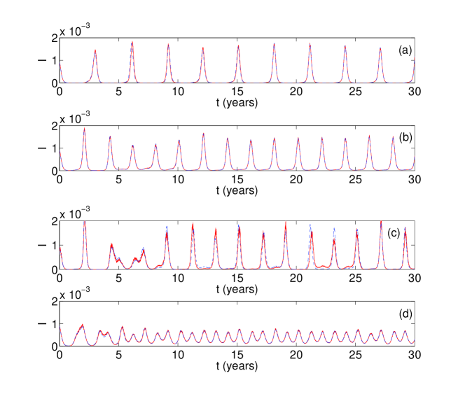
Figure 1: Time series of the fraction of the population that is infected with a disease, $I$. The time series are found using the complete, stochastic system of transformed equations of the SEIR model (red, solid line) as well as the reduced, stochastic system of equations (blue, dashed line). The parameter values used in the simulation are given as (a) $\mu=0.02({\rm year})^{-1}$, $\alpha=1/0.0279({\rm year})^{-1}$, $\gamma=1/0.01({\rm year})^{-1}$, $\beta_{0}=1575.0({\rm year})^{-1}$, $\beta_{1}=0.1$, $\beta_{2}=\zeta_{1}=\zeta_{2}=\omega=0$, and $\sigma=2.0$; (b) the same as in (a) except now $\mu=0.03({\rm year})^{-1}$; (c) the same as in (a) except now $\mu=0.03({\rm year})^{-1}$, $\beta_{1}=0.15$, and $\sigma=5.0$; (d) the same as in (a) except now $\mu=0.04({\rm year})^{-1}$.

Figures 1(a)-(d) compares two time series of the fraction of the population that is infected with a disease, $I$. The first time series was computed using the complete, stochastic system of transformed equations, while the second time series was computed using the reduced, stochastic system of equations. In Fig. 1(a), the following parameter values are used in the computation: $\mu=0.02({\rm year})^{-1}$, $\alpha=1/0.0279({\rm year})^{-1}$, $\gamma=1/0.01({\rm year})^{-1}$, $\beta_{0}=1575.0({\rm year})^{-1}$, $\beta_{1}=0.1$, $\beta_{2}=\zeta_{1}=\zeta_{2}=\omega=0$, and $\sigma=2.0$. These disease parameters correspond to typical measles values (Schwartz and Smith, 1983; Billings and Schwartz, 2002). There is excellent agreement between the two solutions shown in Fig. 1(a). The initial disease outbreak is correctly captured by the reduced model. Furthermore, the reduced model correctly predicts outbreaks for a time scale on the order of decades.

Additionally, the solution found using the reduced, stochastic system agrees very well with the solution found using the complete, stochastic system for a wide range of parameter values. The agreement can be seen in Figs. 1(b)-(d). By changing $\mu$, $\beta_{1}$, and $\sigma$, one can obtain different frequency and amplitude structure of the solutions. Regardless, the reduced system still properly captures the initial disease outbreak as well as the recurring outbreaks.

6 Comparison with Data

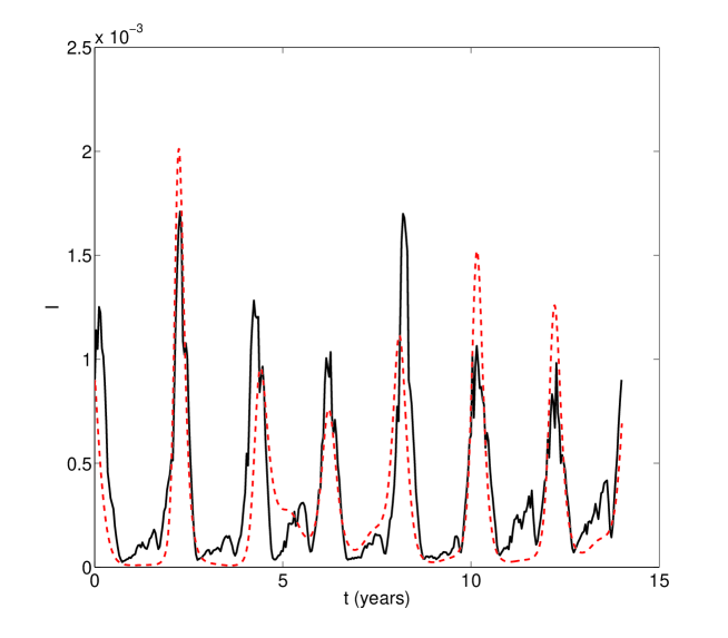
Figure 2: Time series of the fraction of the population that is infected with a disease, $I$. One time series is given by data (Fine and Clarkson, 1982a) from 60 cities in England and Wales over the time span of 1953-1966 (black, solid line), while the other time series is computed using the reduced, stochastic system of equations (red, dashed line) for $\sigma=0.0$ (deterministic). The cross-correlation between the two time series is $0.817$. The parameter values used in the simulation are given as follows: $\mu=0.0299({\rm year})^{-1}$, $\alpha=30.0({\rm year})^{-1}$, $\gamma=90.0({\rm year})^{-1}$, $\beta_{0}=1329.345({\rm year})^{-1}$, $\beta_{1}=0.1$, $\beta_{2}=0.05$, $\zeta_{1}=-0.2128$, $\zeta_{2}=-0.2554$, and $\omega=0.521$.

Measles have been registered on a weekly basis via mandatory notification in the UK (Fine and Clarkson, 1982a), with a reporting rate in the pre-vaccination era better than fifty percent (Clarkson and Fine, 1985). We use existing measles data (Fine and Clarkson, 1982b) that consists of the number of infectious individuals from 60 cities in England and Wales over the 14 year time span of 1953-1966. The data from all of these cities is aggregated so that the total population is 14,602,896. Figure 2 shows the time series of the aggregate data as the fraction of the population that is infected with the disease. Fitting the data with the deterministic version of Eqs. (1a)-(1c) yields the following disease parameter values: $\mu=0.0299({\rm year})^{-1}$, $\alpha=30.0({\rm year})^{-1}$, $\gamma=90.0({\rm year})^{-1}$, $\beta_{0}=1329.345({\rm year})^{-1}$, $\beta_{1}=0.1$, $\beta_{2}=0.05$, $\zeta_{1}=-0.2128$, $\zeta_{2}=-0.2554$, and $\omega=0.521$. Using these parameter values, the reduced system of equations is solved with $\sigma=0.0$ (deterministic case), and the resulting time series is also shown in Fig. 2.

One can see that the agreement between the two time series is quite good. In particular, the reduced system accurately captures the timing of each of the major outbreaks. We also have computed the cross-correlation of the two time series shown in Fig. 2 to be approximately $0.817$. The cross-correlation measures the similarity between the two time series. If the time series were identical, the cross-correlation would be equal to $1.0$. Although the time series of Fig. 2 are not identical, their high cross-correlation value quantitatively suggests good agreement between the measured data and the computed time series.

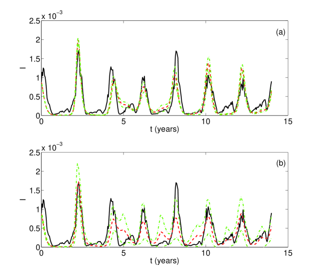
Figure 3: Time series of the fraction of the population that is infected with a disease, $I$. One time series is given by data (Fine and Clarkson, 1982a) (black, solid line), while the other time series is an average solution computed using the reduced, stochastic system of equations (red, dashed line) using $25$ realization of noise with intensity (a) $\sigma=2.0$, and (b) $\sigma=10.0$. The range of $I$ within one standard deviation of the mean also is denoted (green, dashed-dotted line). The cross-correlation between the data time series and the average time series from the reduced model in (a) is $0.810$, while the cross-correlation between the two time series in (b) is $0.655$. The parameter values used in the simulation are given as follows: $\mu=0.0299({\rm year})^{-1}$, $\alpha=30.0({\rm year})^{-1}$, $\gamma=90.0({\rm year})^{-1}$, $\beta_{0}=1329.345({\rm year})^{-1}$, $\beta_{1}=0.1$, $\beta_{2}=0.05$, $\zeta_{1}=-0.2128$, $\zeta_{2}=-0.2554$, and $\omega=0.521$.

The solution that is computed using the reduced, stochastic system is very robust to noise. The standard deviation of the noise intensity $\sigma$ must be fairly large to significantly affect the accuracy of the computed solution. Figure 3(a) compares the data time series with the average time series computed using the reduced, stochastic model with $25$ realizations of noise with intensity $\sigma=2.0$. Figure 3(b) is similar, except that $\sigma=10.0$ was used for the reduced model computation. Also shown in Figs. 3(a)-(b) is the range of infectives that fall within one standard deviation of the average solution.

By comparing Fig. 2 with Fig. 3(a), one can see that the noise has not had a great effect on the mean solution found using the reduced model. In fact, the cross-correlation between the two time series of Fig. 3(a) is approximately $0.810$, which is very near the deterministic cross-correlation value. Beyond $\sigma=2.0$ the noise has a significant degrading effect on the reduced model solution. Figure 3(b) shows that the overall agreement between the two time series is still relatively good. However, by comparing Fig. 3(a) with Fig. 3(b), one can see that the larger noise has led to significant differences between the two reduced model solutions. The cross-correlation value is $0.655$, which is much lower than the cross-correlation found for lower values of $\sigma$.

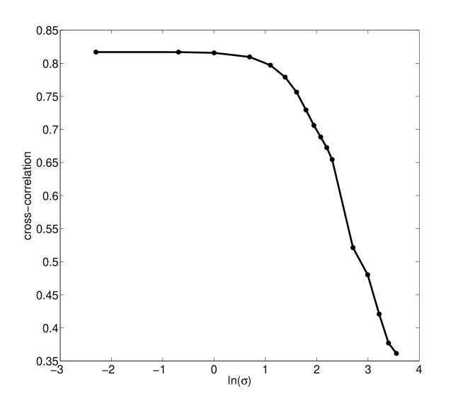
Figure 4: Cross-correlation between the data time series and the time series which is computed using the reduced, stochastic system of equations for noise intensities ranging from $\sigma=0.1$ to $\sigma=35.0$. The cross-correlation for $\sigma=0.0$ (deterministic) is $0.817$ (data point is not shown). For each value of $\sigma$, the data point represents the average of individual cross-correlations computed using $25$ realizations of the noise.

To obtain a comprehensive idea of the effect of the noise, we have computed the cross-correlation between the data time series and the time series computed using the reduced, stochastic system for noise intensities ranging from $\sigma=0.1$ to $\sigma=35.0$. Figure 4 shows the cross-correlation as a function of $\ln{(\sigma)}$.

The reduction method also allows one to predict the unobserved number of exposed individuals based on the observed number of infected individuals. Using the center manifold equation given by Eq. (21) along with the equations which relate the original $S$, $E$, and $I$ variables to the transformed $U$, $V$, and $W$ variables, one can find the following relation between exposed and infected individuals:

$$E=\frac{\gamma}{\alpha}I+\frac{\mu^{2}}{\alpha\beta_{0}}\left(R_{0}-1\right).$$ (23)

In Eq. (23), the first term on the right hand side provides a measure of the statistical steady state flow conditions for exposure and infection, since $\gamma^{-1}$ and $\alpha^{-1}$ are respectively the compartmental recovery and infection times. The second term on the right hand side is a correction, not predicted in the classical theory. An increase in $R_{0}$ leads to an increase in the speed of infection per infectious period. This increase induces an increase in the number of exposed individuals.

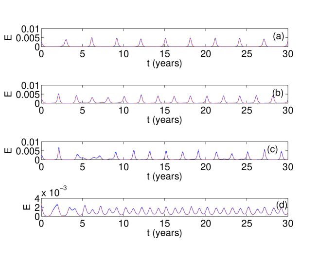
Figure 5: Time series of the fraction of the population that has been exposed to a disease, $E$. The time series are found using the complete, stochastic system of transformed equations of the SEIR model (red, solid line) as well as the predictive equation given by Eq. (23) (blue, dashed line). The parameter values used in the simulation are given as (a) $\mu=0.02({\rm year})^{-1}$, $\alpha=1/0.0279({\rm year})^{-1}$, $\gamma=1/0.01({\rm year})^{-1}$, $\beta_{0}=1575.0({\rm year})^{-1}$, $\beta_{1}=0.1$, $\beta_{2}=\zeta_{1}=\zeta_{2}=\omega=0$, and $\sigma=2.0$; (b) $\mu=0.03({\rm year})^{-1}$, $\alpha=1/0.0279({\rm year})^{-1}$, $\gamma=1/0.01({\rm year})^{-1}$, $\beta_{0}=1575.0({\rm year})^{-1}$, $\beta_{1}=0.1$, $\beta_{2}=\zeta_{1}=\zeta_{2}=\omega=0$, and $\sigma=2.0$; (c) $\mu=0.03({\rm year})^{-1}$, $\alpha=1/0.0279({\rm year})^{-1}$, $\gamma=1/0.01({\rm year})^{-1}$, $\beta_{0}=1575.0({\rm year})^{-1}$, $\beta_{1}=0.15$, $\beta_{2}=\zeta_{1}=\zeta_{2}=\omega=0$, and $\sigma=5.0$; (d) $\mu=0.04({\rm year})^{-1}$, $\alpha=1/0.0279({\rm year})^{-1}$, $\gamma=1/0.01({\rm year})^{-1}$, $\beta_{0}=1575.0({\rm year})^{-1}$, $\beta_{1}=0.1$, $\beta_{2}=\zeta_{1}=\zeta_{2}=\omega=0$, and $\sigma=2.0$.

Figures 5(a)-(d) shows a comparison between time series of the fraction of the population that has been exposed to a disease, $E$. The first time series was computed using the complete, stochastic system of transformed equations. We then used the simulated $I$ data to predict the number of exposed individuals using Eq. (23). The predicted number of exposed individuals constitutes the second time series. This comparison was performed for four different sets of parameter values, corresponding to the values used in Figs. 1(a)-(d). As one can see, there is excellent agreement between the predicted number of exposed individuals and the actual, simulated number of exposed individuals.

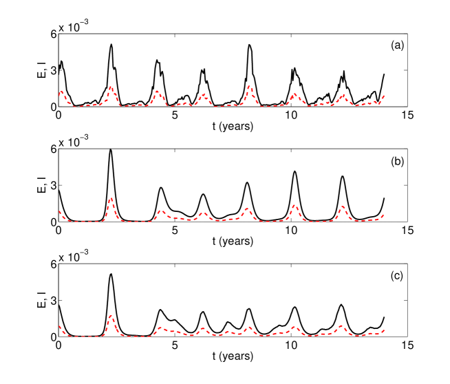
Figure 6: Time series of the fraction of the population that has been exposed to a disease, $E$ (black, solid line) and infected with a disease, $I$ (red, dashed line). The time series of exposed individuals is based on the center manifold equation and is given by Eq. (23). Part (a) shows the observed data of infectious individuals along with the predicted, unobserved number of exposed individuals. Parts (b) and (c) show the average number of infectious individuals computed using the reduced, stochastic system of equations using $25$ realizations of noise with intensity (b) $\sigma=2.0$, and (c) $\sigma=10.0$, along with the associated number of exposed individuals. The parameter values used in the simulation are given as follows: $\mu=0.0299({\rm year})^{-1}$, $\alpha=30.0({\rm year})^{-1}$, $\gamma=90.0({\rm year})^{-1}$, $\beta_{0}=1329.345({\rm year})^{-1}$, $\beta_{1}=0.1$, $\beta_{2}=0.05$, $\zeta_{1}=-0.2128$, $\zeta_{2}=-0.2554$, and $\omega=0.521$.

Figures 6(a)-(c) shows time series of the fraction of the population that has been exposed to a disease, $E$, along with the fraction of infectious individuals, $I$. Fig. 6(a) shows the observed data of infectious individuals and the predicted number of unobserved exposed individuals. Figs. 6(b)-(c) show the average number of infectious individuals computed using the reduced, stochastic system of equations using 25 realizations of noise for two different noise intensities along with the associated number of exposed individuals.

7 Discussion

We have considered a stochastic SEIR model where the contact rate fluctuates seasonally and where multiplicative noise acts on the governing equation for infectious individuals. In this way, we emulated the noise found within data of measurable infectious individuals in a population. The main result of our work was the derivation of a lower-dimensional model whose solution, both in amplitude and timing of outbreaks, agrees with the solution of the higher-dimensional original model.

There are many types of high-dimensional stochastic models which lend themselves to model reduction. For example, a time delay is often included in epidemic models when one wishes to model a disease exposure time. To reduce the analytical complications introduced by the time delay, one can approximate the delay through a cascade of hundreds of exposed compartments (Mocek et al., 2005). Other high dimensional models are generated when individual interactions within a population are modeled as a network (Pastor-Satorras and Vespignani, 2001; Moreno et al., 2002). Researchers have considered epidemics on a variety of static networks, including small world networks (Vazquez, 2006) and transportation networks (Colizza et al., 2006), as well as on adaptive networks, where individuals may break their interaction connections and “rewire” to form new interaction connections (Shaw and Schwartz, 2008).

In these high dimensional model examples, one generally needs to resort to massive computation and analytical results are usually very difficult or impossible to obtain. In particular, it is not currently possible to perform these computations in real-time. However, many high dimensional epidemic models do contain time scales that are well separated. Therefore, it is possible to take advantage of these well-separated time scales to reduce the dimension of the model. In this article we have performed just such a model reduction. The stochastic SEIR model with seasonal fluctuations, which contains fast collapse and slow dynamic time scales, illustrates the power of our method. It is important to note that the analysis could straightforwardly be extended to a SEIR-type model where the exposed class was modeled using hundreds of compartments.

The mathematical/computational techniques used here are general, and can be applied to many population dynamics problems. Our analysis started by transforming the deterministic SEIR system of equations to a new system of equations with a specific eigenvalue structure. Employing center manifold theory, we were able to find the reduced system of equations that describes the dynamics on the lower dimensional manifold. Due to the specific nature of the noise, we can use the deterministic center manifold equation to reduce the stochastic SEIR model. The end result is a reduced stochastic model that accurately captures the timing of the initial disease outbreak as well as the timing of subsequent outbreaks for decades long times compared to the infectious period. The solution to the reduced stochastic model additionally agrees very well in amplitude with the solution to the original high-dimensional model. Moreover, the reduced model is robust in that it accurately captures the timing and amplitude for a wide range of parameter values.

As a direct application to observations, we have also used our deterministic model to fit actual measles data. Once the fitting parameters were determined we solved our reduced stochastic model and compared the resulting solution with the data. Beyond providing good agreement with the data, we saw that a large noise intensity was needed before the stochastic solution significantly deviated from the data. In this way, the stochastic solutions are very robust to noise. We were able to further identify the noise effects through cross-correlation computations.

Generally, the actual data that is measured in society is that of the number of observed cases. Not only are exposed individuals not measured, an exposed individual often will not even know of the exposure and the infection that is to come. However, with our novel stochastic reduction method, we are now able to predict how many unobserved exposed individuals there are in a population based solely on the measurable number of infectious individuals.

In summary, a new method of stochastic model reduction for an epidemiological model with seasonal fluctuations has been performed. By capturing both the timing of disease outbreak as well as the amplitude of the outbreak for long temporal scales, our reduced model provides impressive time series prediction. By accurately modeling actual stochastic disease data, we enable the application of novel control methods where the timing of vaccine delivery and a disease outbreak is important. Moreover, the method is general, and may be extended to a variety of compartmental and network models, including models with a high dimension.

Appendix A Deterministic Model Reduction

The $F_{1}$, $F_{2}$, and $F_{3}$ expressions found in Eqs. (13a)-(13c) are given as follows:

$$F_{1}(U,V,W,\mu)= {\frac{\mu\,\gamma_{0}\,\left(\beta(t)-\beta_{0}\right)\left[-\beta_{0}\,\mu\,\alpha_{0}+\left(\alpha_{0}+{\mu}^{2}\right)\left(\gamma_{0}+{\mu}^{2}\right)\right]}{{\beta_{0}}^{2}\alpha_{0}\,\left(\alpha_{0}+\gamma_{0}\right)}}+$$

$$\left(-\alpha_{0}-{\mu}^{2}-{\frac{\left(\alpha_{0}+{\mu}^{2}\right)\left(\gamma_{0}+{\mu}^{2}\right)\beta(t)}{\beta_{0}\,\alpha_{0}}}+{\frac{{\mu}^{2}\gamma_{0}\,\beta(t)}{\beta_{0}\,\left(\alpha_{0}+\gamma_{0}\right)}}-{\frac{\beta(t)\,{\mu}^{3}\gamma_{0}\,\alpha_{0}}{\left(\alpha_{0}+{\mu}^{2}\right)\left(\gamma_{0}+{\mu}^{2}\right)\left(\alpha_{0}+\gamma_{0}\right)}}\right)U+$$

$$\left(-{\frac{\beta(t)\,{\mu}^{3}\gamma_{0}\,\alpha_{0}}{\left(\alpha_{0}+{\mu}^{2}\right)\left(\gamma_{0}+{\mu}^{2}\right)\left(\alpha_{0}+\gamma_{0}\right)}}+{\frac{{\mu}^{2}\gamma_{0}\,\beta(t)}{\beta_{0}\,\left(\alpha_{0}+\gamma_{0}\right)}}\right)V-{\frac{\gamma_{0}\,\beta(t)\,\left(\gamma_{0}+{\mu}^{2}\right)\left(\alpha_{0}+{\mu}^{2}\right)W}{\alpha_{0}\,\left(\alpha_{0}+\gamma_{0}\right)\beta_{0}}}-$$

$${\frac{\gamma_{0}\,\beta(t)\,\mu\,W\,U}{\alpha_{0}+\gamma_{0}}}-\beta(t)\,\mu\,U\,V-{\frac{\gamma_{0}\,\beta(t)\,\mu\,V\,W}{\alpha_{0}+\gamma_{0}}}-\beta(t)\,\mu\,{U}^{2},$$ (24a)

$$F_{2}(U,V,W,\mu)= {\frac{\mu\,\left(\beta(t)-\beta_{0}\right)\left[-\beta_{0}\,\mu\,\alpha_{0}+\left(\alpha_{0}+{\mu}^{2}\right)\left(\gamma_{0}+{\mu}^{2}\right)\right]}{{\beta_{0}}^{2}\left(\alpha_{0}+\gamma_{0}\right)}}+$$

$$\left(-{\frac{\left(\alpha_{0}+{\mu}^{2}\right)\left(\gamma_{0}+{\mu}^{2}\right)\beta(t)}{\beta_{0}\,\gamma_{0}}}+{\frac{\alpha_{0}\,{\mu}^{2}\beta(t)}{\beta_{0}\,\left(\alpha_{0}+\gamma_{0}\right)}}+\alpha_{0}-{\frac{\beta(t)\,{\mu}^{3}{\alpha_{0}}^{2}}{\left(\alpha_{0}+{\mu}^{2}\right)\left(\gamma_{0}+{\mu}^{2}\right)\left(\alpha_{0}+\gamma_{0}\right)}}\right)U+$$

$$\left(-{\mu}^{2}+{\frac{\alpha_{0}\,{\mu}^{2}\beta(t)}{\beta_{0}\,\left(\alpha_{0}+\gamma_{0}\right)}}-{\frac{\beta(t)\,{\mu}^{3}{\alpha_{0}}^{2}}{\left(\alpha_{0}+{\mu}^{2}\right)\left(\gamma_{0}+{\mu}^{2}\right)\left(\alpha_{0}+\gamma_{0}\right)}}\right)V-{\frac{\left(\alpha_{0}+{\mu}^{2}\right)\left(\gamma_{0}+{\mu}^{2}\right)\beta(t)\,W}{\beta_{0}\,\left(\alpha_{0}+\gamma_{0}\right)}}-$$

$${\frac{\beta(t)\,\alpha_{0}\,\mu\,W\,U}{\alpha_{0}+\gamma_{0}}}-{\frac{\beta(t)\,\alpha_{0}\,\mu\,U\,V}{\gamma_{0}}}-{\frac{\beta(t)\,\alpha_{0}\,\mu\,V\,W}{\alpha_{0}+\gamma_{0}}}-{\frac{\beta(t)\,\alpha_{0}\,\mu\,{U}^{2}}{\gamma_{0}}},$$ (24b)

$$F_{3}(U,V,W,\mu)= -{\frac{\mu\,\left(\beta(t)-\beta_{0}\right)\left[-\beta_{0}\,\mu\,\alpha_{0}+\left(\alpha_{0}+{\mu}^{2}\right)\left(\gamma_{0}+{\mu}^{2}\right)\right]}{\alpha_{0}\,{\beta_{0}}^{2}}}+$$

$$\left({\frac{\beta(t)\,\left(\alpha_{0}+{\mu}^{2}\right)\left(\gamma_{0}+{\mu}^{2}\right)\left(\alpha_{0}+\gamma_{0}\right)}{\beta_{0}\,\alpha_{0}\,\gamma_{0}}}-{\frac{\beta(t)\,{\mu}^{2}}{\beta_{0}}}-\alpha_{0}-\gamma_{0}+{\frac{{\mu}^{3}\beta(t)\,\alpha_{0}}{\left(\alpha_{0}+{\mu}^{2}\right)\left(\gamma_{0}+{\mu}^{2}\right)}}\right)U+$$

$$\left(-{\frac{\beta(t)\,{\mu}^{2}}{\beta_{0}}}+{\frac{{\mu}^{3}\beta(t)\,\alpha_{0}}{\left(\alpha_{0}+{\mu}^{2}\right)\left(\gamma_{0}+{\mu}^{2}\right)}}\right)V+{\frac{\left(\gamma_{0}+{\mu}^{2}\right)\left(\beta(t)\,\alpha_{0}+\beta(t)\,{\mu}^{2}-\beta_{0}\,\alpha_{0}\right)W}{\beta_{0}\,\alpha_{0}}}+$$

$$\beta(t)\,\mu\,W\,U+{\frac{\beta(t)\,\mu\,\left(\alpha_{0}+\gamma_{0}\right)U\,V}{\gamma_{0}}}+\beta(t)\,\mu\,V\,W+{\frac{\beta(t)\,\mu\,\left(\alpha_{0}+\gamma_{0}\right){U}^{2}}{\gamma_{0}}}.$$ (24c)

Appendix B Stochastic Model Reduction

The stochastic, transformed equations are given as follows:

$$\frac{dU}{d\tau}= {\frac{\mu\,\gamma_{0}\,\left(\beta(t)-\beta_{0}\right)\left[-\beta_{0}\,\mu\,\alpha_{0}+\left(\alpha_{0}+{\mu}^{2}\right)\left(\gamma_{0}+{\mu}^{2}\right)\right]}{{\beta_{0}}^{2}\alpha_{0}\,\left(\alpha_{0}+\gamma_{0}\right)}}+$$

$$\left(-\alpha_{0}-{\mu}^{2}-{\frac{\left(\alpha_{0}+{\mu}^{2}\right)\left(\gamma_{0}+{\mu}^{2}\right)\beta(t)}{\beta_{0}\,\alpha_{0}}}+{\frac{{\mu}^{2}\gamma_{0}\,\beta(t)}{\beta_{0}\,\left(\alpha_{0}+\gamma_{0}\right)}}-{\frac{\beta(t)\,{\mu}^{3}\gamma_{0}\,\alpha_{0}}{\left(\alpha_{0}+{\mu}^{2}\right)\left(\gamma_{0}+{\mu}^{2}\right)\left(\alpha_{0}+\gamma_{0}\right)}}\right)U+$$

$$\left(-{\frac{\beta(t)\,{\mu}^{3}\gamma_{0}\,\alpha_{0}}{\left(\alpha_{0}+{\mu}^{2}\right)\left(\gamma_{0}+{\mu}^{2}\right)\left(\alpha_{0}+\gamma_{0}\right)}}+{\frac{{\mu}^{2}\gamma_{0}\,\beta(t)}{\beta_{0}\,\left(\alpha_{0}+\gamma_{0}\right)}}\right)V-{\frac{\gamma_{0}\,\beta(t)\,\left(\gamma_{0}+{\mu}^{2}\right)\left(\alpha_{0}+{\mu}^{2}\right)W}{\alpha_{0}\,\left(\alpha_{0}+\gamma_{0}\right)\beta_{0}}}-$$

$${\frac{\gamma_{0}\,\beta(t)\,\mu\,W\,U}{\alpha_{0}+\gamma_{0}}}-\beta(t)\,\mu\,U\,V-{\frac{\gamma_{0}\,\beta(t)\,\mu\,V\,W}{\alpha_{0}+\gamma_{0}}}-\beta(t)\,\mu\,{U}^{2},$$ (25a)

$$\frac{dV}{d\tau}= {\frac{\mu\,\left(\beta(t)-\beta_{0}\right)\left[-\beta_{0}\,\mu\,\alpha_{0}+\left(\alpha_{0}+{\mu}^{2}\right)\left(\gamma_{0}+{\mu}^{2}\right)\right]}{{\beta_{0}}^{2}\left(\alpha_{0}+\gamma_{0}\right)}}+$$

$$\left(-{\frac{\left(\alpha_{0}+{\mu}^{2}\right)\left(\gamma_{0}+{\mu}^{2}\right)\beta(t)}{\beta_{0}\,\gamma_{0}}}+{\frac{\alpha_{0}\,{\mu}^{2}\beta(t)}{\beta_{0}\,\left(\alpha_{0}+\gamma_{0}\right)}}+\alpha_{0}-{\frac{\beta(t)\,{\mu}^{3}{\alpha_{0}}^{2}}{\left(\alpha_{0}+{\mu}^{2}\right)\left(\gamma_{0}+{\mu}^{2}\right)\left(\alpha_{0}+\gamma_{0}\right)}}\right)U+$$

$$\left(-{\mu}^{2}+{\frac{\alpha_{0}\,{\mu}^{2}\beta(t)}{\beta_{0}\,\left(\alpha_{0}+\gamma_{0}\right)}}-{\frac{\beta(t)\,{\mu}^{3}{\alpha_{0}}^{2}}{\left(\alpha_{0}+{\mu}^{2}\right)\left(\gamma_{0}+{\mu}^{2}\right)\left(\alpha_{0}+\gamma_{0}\right)}}\right)V-{\frac{\left(\alpha_{0}+{\mu}^{2}\right)\left(\gamma_{0}+{\mu}^{2}\right)\beta(t)\,W}{\beta_{0}\,\left(\alpha_{0}+\gamma_{0}\right)}}-$$

$${\frac{\beta(t)\,\alpha_{0}\,\mu\,W\,U}{\alpha_{0}+\gamma_{0}}}-{\frac{\beta(t)\,\alpha_{0}\,\mu\,U\,V}{\gamma_{0}}}-{\frac{\beta(t)\,\alpha_{0}\,\mu\,V\,W}{\alpha_{0}+\gamma_{0}}}-{\frac{\beta(t)\,\alpha_{0}\,\mu\,{U}^{2}}{\gamma_{0}}},$$ (25b)

$$\frac{dW}{d\tau}= -{\frac{\mu\,\left(\beta(t)-\beta_{0}\right)\left[-\beta_{0}\,\mu\,\alpha_{0}+\left(\alpha_{0}+{\mu}^{2}\right)\left(\gamma_{0}+{\mu}^{2}\right)\right]}{\alpha_{0}\,{\beta_{0}}^{2}}}+$$

$$\left({\frac{\beta(t)\,\left(\alpha_{0}+{\mu}^{2}\right)\left(\gamma_{0}+{\mu}^{2}\right)\left(\alpha_{0}+\gamma_{0}\right)}{\beta_{0}\,\alpha_{0}\,\gamma_{0}}}-{\frac{\beta(t)\,{\mu}^{2}}{\beta_{0}}}-\alpha_{0}-\gamma_{0}+{\frac{{\mu}^{3}\beta(t)\,\alpha_{0}}{\left(\alpha_{0}+{\mu}^{2}\right)\left(\gamma_{0}+{\mu}^{2}\right)}}\right)U+$$

$$\left(-{\frac{\beta(t)\,{\mu}^{2}}{\beta_{0}}}+{\frac{{\mu}^{3}\beta(t)\,\alpha_{0}}{\left(\alpha_{0}+{\mu}^{2}\right)\left(\gamma_{0}+{\mu}^{2}\right)}}\right)V+{\frac{\left(\gamma_{0}+{\mu}^{2}\right)\left(\beta(t)\,\alpha_{0}+\beta(t)\,{\mu}^{2}-\beta_{0}\,\alpha_{0}\right)W}{\beta_{0}\,\alpha_{0}}}+$$

$$\beta(t)\,\mu\,W\,U+{\frac{\beta(t)\,\mu\,\left(\alpha_{0}+\gamma_{0}\right)U\,V}{\gamma_{0}}}+\beta(t)\,\mu\,V\,W+{\frac{\beta(t)\,\mu\,\left(\alpha_{0}+\gamma_{0}\right){U}^{2}}{\gamma_{0}}}+$$

$$\mu\sigma\left(\frac{(\alpha_{0}+\gamma_{0})}{\gamma_{0}}U+W+I_{0}\right)\phi,$$ (25c)

As discussed in the article, we can use the deterministic center manifold result to reduce the stochastic model. Substituting the deterministic center manifold equation given by Eq. (21) into the full system of stochastic, transformed equations gives the following reduced stochastic model that describes the dynamics on the center manifold:

$$\frac{dV}{d\tau}= {\frac{\mu\,\left({\beta(t)}-{\beta_{0}}\right)\left[-{\beta_{0}}\,\mu\,{\alpha_{0}}+\left({\alpha_{0}}+{\mu}^{2}\right)\left({\gamma_{0}}+{\mu}^{2}\right)\right]}{{{\beta_{0}}}^{2}\left({\alpha_{0}}+{\gamma_{0}}\right)}}+$$

$$\left(-{\frac{\left({\alpha_{0}}+{\mu}^{2}\right)\left({\gamma_{0}}+{\mu}^{2}\right){\beta(t)}}{{\beta_{0}}\,{\gamma_{0}}}}+{\frac{{\alpha_{0}}\,{\mu}^{2}{\beta(t)}}{{\beta_{0}}\,\left({\alpha_{0}}+{\gamma_{0}}\right)}}+{\alpha_{0}}-{\frac{{\beta(t)}\,{\mu}^{3}{{\alpha_{0}}}^{2}}{\left({\alpha_{0}}+{\mu}^{2}\right)\left({\gamma_{0}}+{\mu}^{2}\right)\left({\alpha_{0}}+{\gamma_{0}}\right)}}\right){\left(-\frac{\gamma_{0}^{2}}{\left(\alpha_{0}+\gamma_{0}\right)^{2}}W\right)}+$$

$$\left(-{\mu}^{2}+{\frac{{\alpha_{0}}\,{\mu}^{2}{\beta(t)}}{{\beta_{0}}\,\left({\alpha_{0}}+{\gamma_{0}}\right)}}-{\frac{{\beta(t)}\,{\mu}^{3}{{\alpha_{0}}}^{2}}{\left({\alpha_{0}}+{\mu}^{2}\right)\left({\gamma_{0}}+{\mu}^{2}\right)\left({\alpha_{0}}+{\gamma_{0}}\right)}}\right){V}-{\frac{\left({\alpha_{0}}+{\mu}^{2}\right)\left({\gamma_{0}}+{\mu}^{2}\right){\beta(t)}\,{W}}{{\beta_{0}}\,\left({\alpha_{0}}+{\gamma_{0}}\right)}}-$$

$${\frac{{\beta(t)}\,{\alpha_{0}}\,\mu\,{W}\,{\left(-\frac{\gamma_{0}^{2}}{\left(\alpha_{0}+\gamma_{0}\right)^{2}}W\right)}}{{\alpha_{0}}+{\gamma_{0}}}}-{\frac{{\beta(t)}\,{\alpha_{0}}\,\mu\,{\left(-\frac{\gamma_{0}^{2}}{\left(\alpha_{0}+\gamma_{0}\right)^{2}}W\right)}\,{V}}{{\gamma_{0}}}}-{\frac{{\beta(t)}\,{\alpha_{0}}\,\mu\,{\it We}\,{W}}{{\alpha_{0}}+{\gamma_{0}}}}-{\frac{{\beta(t)}\,{\alpha_{0}}\,\mu\,{{\left(-\frac{\gamma_{0}^{2}}{\left(\alpha_{0}+\gamma_{0}\right)^{2}}W\right)}}^{2}}{{\gamma_{0}}}},$$ (26a)

$$\frac{dW}{d\tau}= -{\frac{\mu\,\left({\beta(t)}-{\beta_{0}}\right)\left(-{\beta_{0}}\,\mu\,{\alpha_{0}}+\left({\alpha_{0}}+{\mu}^{2}\right)\left({\gamma_{0}}+{\mu}^{2}\right)\right)}{{\alpha_{0}}\,{{\beta_{0}}}^{2}}}+$$

$$\left({\frac{{\beta(t)}\,\left({\alpha_{0}}+{\mu}^{2}\right)\left({\gamma_{0}}+{\mu}^{2}\right)\left({\alpha_{0}}+{\gamma_{0}}\right)}{{\beta_{0}}\,{\alpha_{0}}\,{\gamma_{0}}}}-{\frac{{\beta(t)}\,{\mu}^{2}}{{\beta_{0}}}}-{\alpha_{0}}-{\gamma_{0}}+{\frac{{\mu}^{3}{\beta(t)}\,{\alpha_{0}}}{\left({\alpha_{0}}+{\mu}^{2}\right)\left({\gamma_{0}}+{\mu}^{2}\right)}}\right){\it\left(-\frac{\gamma_{0}^{2}}{\left(\alpha_{0}+\gamma_{0}\right)^{2}}W\right)}+$$

$$\left(-{\frac{{\beta(t)}\,{\mu}^{2}}{{\beta_{0}}}}+{\frac{{\mu}^{3}{\beta(t)}\,{\alpha_{0}}}{\left({\alpha_{0}}+{\mu}^{2}\right)\left({\gamma_{0}}+{\mu}^{2}\right)}}\right){V}+{\frac{\left({\gamma_{0}}+{\mu}^{2}\right)\left({\beta(t)}\,{\alpha_{0}}+{\beta(t)}\,{\mu}^{2}-{\beta_{0}}\,{\alpha_{0}}\right){W}}{{\beta_{0}}\,{\alpha_{0}}}}+$$

$${\beta(t)}\,\mu\,{W}\,{\it\left(-\frac{\gamma_{0}^{2}}{\left(\alpha_{0}+\gamma_{0}\right)^{2}}W\right)}+{\frac{{\beta(t)}\,\mu\,\left({\alpha_{0}}+{\gamma_{0}}\right){\left(-\frac{\gamma_{0}^{2}}{\left(\alpha_{0}+\gamma_{0}\right)^{2}}W\right)}\,{V}}{{\gamma_{0}}}}+{\beta(t)}\,\mu\,{V}\,{W}+$$

$${\frac{{\beta(t)}\,\mu\,\left({\alpha_{0}}+{\gamma_{0}}\right){{\left(-\frac{\gamma_{0}^{2}}{\left(\alpha_{0}+\gamma_{0}\right)^{2}}W\right)}}^{2}}{{\gamma_{0}}}}+\mu\sigma\left(\frac{(\alpha_{0}+\gamma_{0})}{\gamma_{0}}U+W+I_{0}\right)\phi.$$ (26b)