Non-Linear Localized Modes Give Rise to a Reflective Optical Limiter

Abstract

Optical limiters are designed to transmit low intensity light, while blocking the light with excessively high intensity. A typical passive limiter absorbs excessive electromagnetic energy, which can cause its overheating and destruction. We propose the concept of a layered reflective limiter based on resonance transmission via a non-linear localized mode. Such a limiter does not absorb the high level radiation, but rather reflects it back to space. Importantly, the total reflection occurs within a broad frequency range and for an arbitrary direction of incidence. The same concept can be applied to infrared and microwave frequencies.

The continuing integration of optical devices into modern technology has led to the development of an ever increasing number of novel schemes for efficiently manipulating the amplitude, phase, polarization, or direction of optical beams ST91 . Among these manipulations, the ability to control the intensity of light in a predetermined manner is of the utmost importance, with applications ranging from optical communications to optical computing O97 ; PHR98 and sensoring. As laser technology is making progress, novel protection devices (optical limiters) are needed to protect optical sensors and other components from high-power laser damage limiter1 ; limiter2 ; limiter3 .

Here we focus on the most popular, passive optical limiters. The simplest realization of a passive optical limiter is provided by a single nonlinear layer with the imaginary part $n^{\prime\prime}$ of the refractive index being dependent on the light intensity $W$. At low intensity, the value $n^{\prime\prime}(W)$ is relatively small, and the nonlinear layer is transparent. As the light intensity exceeds certain level, the value $n^{\prime\prime}(W)$ increases dramatically, and the nonlinear protective layer turns opaque. In more sophisticated schemes, the nonlinear layer can be a part of a complicated optical setup. The problem though is that in all cases, the limiter absorbs the excessive power, which might cause overheating or even destruction of the device (a sacrificial limiter). Our goal is, using the existing nonlinear materials, to design a photonic structure which would reflect the excessive power back to space, rather than absorbing it. Such a structure can be referred to as a passive reflective limiter. A free- space realization of a reflective limiter is a layered array reflecting a high intensity light regardless of the direction of incidence and within a broad frequency range.

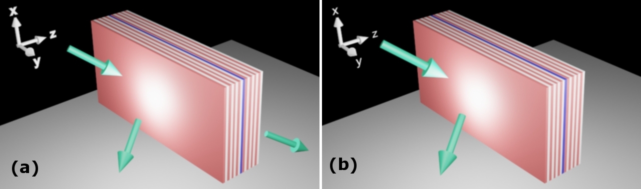
Figure 1: (Color online) A power limiter consisting of a non-linear lossy layer (blue layer) embedded in a Bragg grating (white and orange layers). This set-up allows for (a) a transmission of a low intensity beam while (b) it completely reflects a high intensity beam without any absorption.

Our proposal is based on resonance transmission through a nonlinear localized mode. The simplest realization of the above idea is illustrated in Fig. 1, where a nonlinear lossy layer is sandwiched between two linear lossless Bragg reflectors. We will show that if the light intensity is low, the absorption can be small, and the layered structure in Fig. 1 will be transmissive in the vicinity of the localized mode frequency. If the incident light intensity exceeds a certain level, the non-linear layer in Fig. 1 decouples the two Bragg gratings and the entire stack becomes highly reflective – not opaque, as in the case of a stand-alone nonlinear layer. In other words, the high intensity light will be reflected back to space, rather than absorbed by the limiter. Even this simple design provides a broad band protection for an arbitrary direction of incidence. For a given nonlinear material, the intensity limitation of the transmitted light can be controlled by adjusting the layered structure, so that the electromagnetic energy density in the vicinity of the nonlinear layer is either enhanced or attenuated. A problem with the simple design of Fig. 1 is that the low-intensity transmittance only occurs in the vicinity of the localized mode frequency. This problem can be addressed by using more sophisticated photonic structures, for instance, those involving two or more coupled defect layers, as it is done in the case of optical filters M01 .

To illustrate our idea, we consider a pair of identical Bragg gratings, each consisting of two alternating layers with real permittivities $\epsilon_{1}$ and $\epsilon_{2}$, placed in the intervals $-L\leq z\leq 0$ and $d_{\gamma}\leq z\leq L+d_{\gamma}$. The width of each grating layer is $d$. A non-linear lossy layer of width $d_{\gamma}$ is placed between the two gratings at $0\leq z\leq d_{\gamma}$; its complex permittivity $\epsilon_{\gamma}=\epsilon(1+i\gamma|E(z)|^{2})$ is field dependent. In the particular case of $\epsilon=\epsilon_{1}$ and $\gamma=0$, we have a standard Bragg grating with a band-gap around the frequency $\omega_{B}=c/(n_{0}d)$ ($c$ is the speed of light). The defect layer creates a localized mode with the frequency $\omega_{r}$ lying within a photonic band-gap. At this frequency, the entire stack displays resonance transmission accompanied by a dramatic field enhancement in the vicinity of the defect layer. The enhanced field, in turn, causes the respective increase in the imaginary part of the defect layer permittivity, $\epsilon_{\gamma}$. The latter will eventually result in decoupling of the two Bragg reflectors and rendering the entire structure in Fig. 1 highly reflective.

We first consider normal incidence. In this arrangement, a time-harmonic electric field of frequency $\omega$ obeys the Helmholtz equation:

$${\frac{\partial^{2}E(z)}{\partial z^{2}}}+{\frac{\omega^{2}}{c^{2}}}\epsilon(z)E(z)=0\,\,\,.$$ (1)

Eq. (1) admits the solution $E_{0}^{-}(z)=E_{f}^{-}\exp(ikz)+E_{b}^{-}\exp(-ikz)$ for $z<-L$ and $E_{0}^{+}(z)=E_{f}^{+}\exp(ikz)+E_{b}^{+}\exp(-ikz)$ for $z>L+d_{\gamma}$ where the wavevector $k=n_{0}\omega/c$. The transmittance, reflectance and absorption, say for a left incident wave, are then defined as $\mathcal{T}=|E_{f}^{+}/E_{f}^{-}|^{2}$; $\mathcal{R}=|E_{b}^{-}/E_{f}^{-}|^{2}$; and $\mathcal{A}=1-\mathcal{T}-\mathcal{R}$ respectively note1 . They can be calculated numerically using a backward map approach.

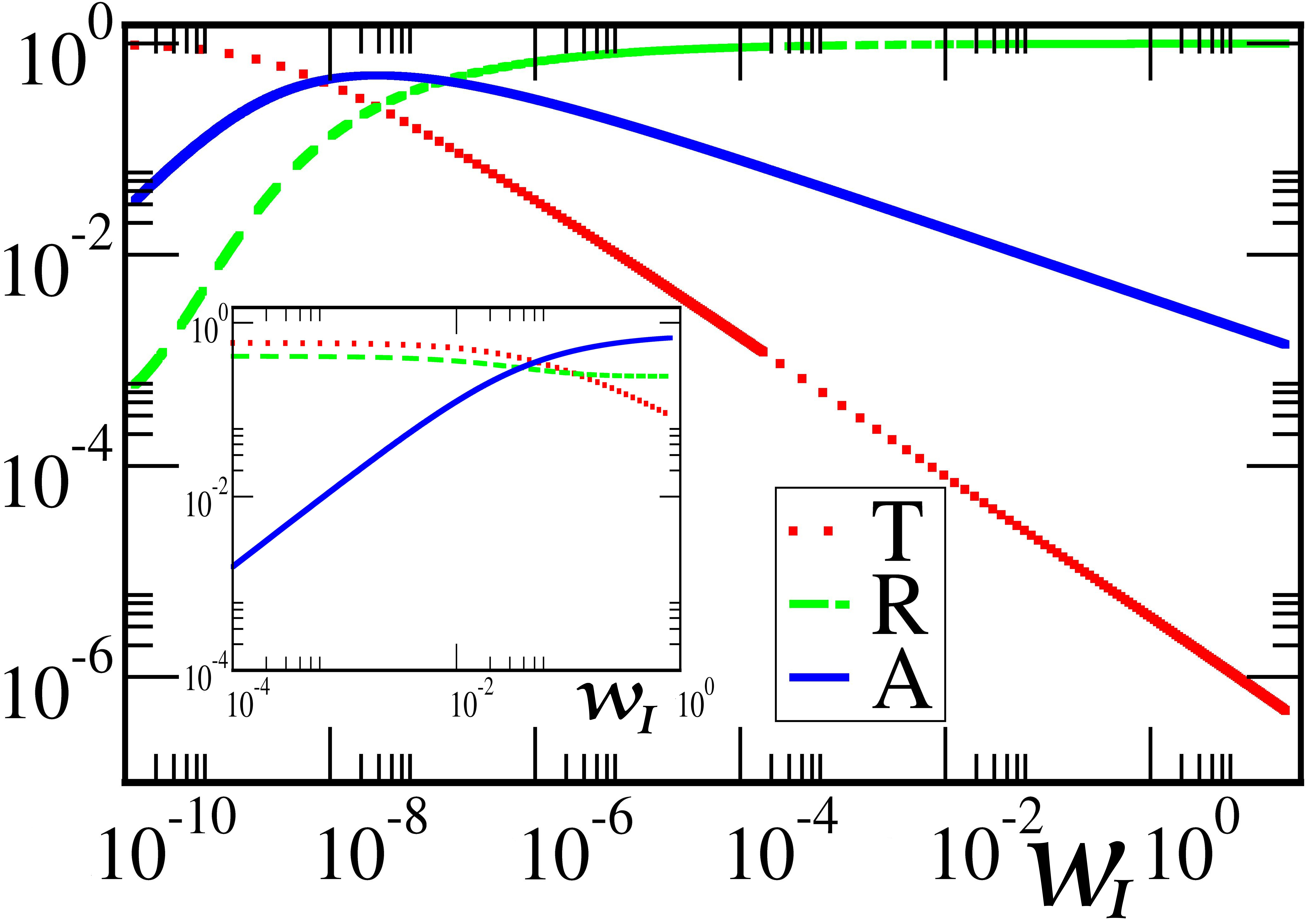
Figure 2: Normal incidence for the structure of Fig. 1. We report the transmittance $\mathcal{T}$, absorption $\mathcal{A}$ and reflectance $\mathcal{R}$, as a function of the incident power $\mathcal{W}_{I}$ at a resonant frequency $\omega_{r}\approx 8.15$. The parameters of the grating are indicated at the text. We observe that for moderate values of $\mathcal{W}_{I}$, both $\mathcal{T}$ and $\mathcal{A}$ are suppressed and the system becomes reflective i.e. $R\approx 1$. Inset: $\mathcal{T}$, $\mathcal{A}$, $\mathcal{R}$ for a single non-linear layer (normal incidence). This system, for moderate $\mathcal{W}_{I}$-values, does not reflect but mainly absorbs the incident energy.

The amplitudes of forward and backward propagating waves on the left $z<-L$ (right $z>L+d_{\gamma}$) domains outside of the grating are related to the ones before (after) the non-linear impurity layer by the algebraic relations:

$$\left(\begin{array}[]{c}E_{f}^{b}\\ E_{b}^{b}\end{array}\right)=M^{(L)}\left(\begin{array}[]{c}E_{f}^{-}\\ E_{b}^{-}\end{array}\right);\,\,\left(\begin{array}[]{c}E_{f}^{+}\\ E_{b}^{+}\end{array}\right)=M^{(R)}\left(\begin{array}[]{c}E_{f}^{a}\\ E_{b}^{a}\end{array}\right)$$ (2)

where $M^{(L)}$ ($M^{(R)}$) are the $2\times 2$ transfer matrices of the optical structure associated with the domain $-L\leq z\leq 0$ ($d_{\gamma}\leq z\leq L+d_{\gamma}$). Above we have expressed the field before (after) the nonlinear layer as $E^{b}=E_{f}^{b}\exp(ikz)+E_{b}^{b}\exp(-ikz)$ ($E^{a}=E_{f}^{a}\exp(ikz)+E_{b}^{a}\exp(-ikz)$). The field $E^{a}(z=d_{\gamma})$ and its derivative $(dE^{a}/dz)|_{z=d_{\gamma}}$ just after the non-linear layer is then evaluated using $M^{(R)}$ from Eq. (2) together with the boundary conditions (associated with a left incident wave) $E_{b}^{+}=0$ and $E_{f}^{+}=1$. Using $E^{a}(z=d_{\gamma})$ and $(dE^{a}(z)/dz)|_{z=d_{\gamma}}$ as initial conditions we have integrated backwards Eq. (1), with the help of a 4rth order Runge-Kutta, and obtained the field $E^{b}(z=0)$ and its derivative $(dE^{b}/dz)|_{z=0}$ at the other end $z=0$ of the nonlinear layer. From these values we evaluate the forward $E_{f}^{b}$ and backward $E_{b}^{b}$ propagating amplitudes. Utilizing Eq. (2) together with $M^{(L)}$ we finally find the amplitudes $E_{f}^{-}$ and $E_{b}^{-}$ which allow us to calculate $\mathcal{T},\mathcal{R}$ and $\mathcal{A}$. Note that for a backward map with boundary condition $E_{f}^{+}=1$ we have $|E_{f}^{-}|^{2}=1/\mathcal{T}$.

It is convenient to work with the rescaled variable ${\tilde{E}}(z)=\sqrt{\gamma}E$. In this representation, Eq. (1) becomes

$${\frac{\partial^{2}{\tilde{E}}(z)}{\partial z^{2}}}+{\frac{\omega^{2}}{c^{2}}}{\tilde{\epsilon}}(z){\tilde{E}}(z)=0\,\,\,$$ (3)

where ${\tilde{\epsilon}}(z\notin[0,d_{\gamma}])=\epsilon(z)$, while ${\tilde{\epsilon}}(z\in[0,d_{\gamma}])=\epsilon_{\gamma}(1+i|{\tilde{E}}(z)|^{2})$. In other words, in this representation, the non-linear layer has a fixed absorption rate which is equal to unity, the outgoing field boundary associated with the backward map varies as ${\tilde{E}}_{f}^{+}=\sqrt{\gamma}$ while the incident light intensity $\mathcal{W}_{I}$ is $\mathcal{W}_{I}\equiv|{\tilde{E}}_{f}^{-}|^{2}=\gamma/\mathcal{T}=\gamma|E_{f}^{-}|^{2}$.

In Fig. 2, the effect of the incident intensity $\mathcal{W}_{I}$ on the transmission, reflection and absorption of a resonant localized mode is presented. The Bragg grating used in these simulations consists of 40 layers on each side with alternating permittivities $\epsilon_{1}=4$ and $\epsilon_{2}=9$. The width of the impurity layer is $d_{\gamma}=1$ and the amplitude $\epsilon$ of the nonlinear permittivity is $\epsilon=9$. We have confirmed numerically that in the linear case the defect creates a resonant mode at $\omega_{r}\approx 8.15$ note4 at the band-gap of the grating which is localized around the impurity. We find that as the incident intensity $\mathcal{W}_{I}$ increases (main panel of Fig. 2), the transmittance of this resonant mode decreases, with a simultaneous increase of the absorption. Further increase of $\mathcal{W}_{I}$, results in noticeable growth of the reflectance with a simultaneous decrease of the absorption and transmittance. Eventually both $\mathcal{T}$ and $\mathcal{A}$ vanishes for moderate values of $\mathcal{W}_{I}$. In other words the system reflects completely the incident radiation. For the shake of comparison we also calculated $\mathcal{T},\mathcal{A}$ and $\mathcal{R}$ versus $\mathcal{W}_{I}$ for a single non-linear layer with no Bragg reflectors (see inset of Fig. 2). We find that for the same range of moderate values of incident intensity $\mathcal{W}_{I}$, the system rather absorbs the energy instead of reflecting it back to space.

For normal incidence, a further theoretical analysis can be carried out. To this end we assume that the permittivity of the non-linear layer is $\epsilon_{\gamma}(z)=\epsilon(1+i\gamma|E(z)|^{2})\delta(z)$. This approximation is justified in the case of a thin metallic defect. For the analytical calculation of $\mathcal{T},\mathcal{R}$ and $\mathcal{A}$, we proceed along the same lines that we have highlighted in the numerical analysis previously. For the sake of generality we will assume that the transport characteristics of the left and right linear subsystems are encoded in the values of their left (right) transmission $t_{L}(t_{R})$ and reflection $r_{L}(r_{R})$ amplitudes. The elements of the transfer matrices $M^{(L)}$ and $M^{(R)}$ (see Eq. (2)) are defined as $M_{11}^{(L/R)}=1/t_{L/R}^{*}$, $M_{12}^{(L/R)}=-r_{L/R}/t_{L/R}$, $M_{21}^{(L/R)}=-(r_{L/R}/t_{L/R})^{*}$, and $M_{22}^{(L/R)}=1/t_{L/R}$.

Next we calculate the field amplitudes just before and after the delta defect by utilizing the transfer matrices Eq.(2) associated with the linear segments. For a left incident wave, we have at $z=0^{-}$

$$E_{f}^{b}=\frac{E_{f}^{-}}{t_{L}^{*}}-\frac{r_{L}E_{f}^{+}}{t_{L}};\quad E_{b}^{b}=\frac{E_{f}^{+}}{t_{L}}-\frac{E_{f}^{-}r_{L}^{*}}{t_{L}^{*}}$$ (4)

while at $z=0^{+}$ just after the delta defect we have

$$E_{f}^{a}=\frac{t_{R}^{*}E_{f}^{+}}{1-|r_{R}|^{2}};\quad E_{b}^{a}=\frac{t_{R}r_{R}^{*}E_{f}^{+}}{1-|r_{R}|^{2}}.$$ (5)

Using Eqs. (4,5) together with the continuity of the field at $z=0$ and the suitable discontinuity of its derivative we write the incident and reflected field amplitudes in terms of the transmitted wave amplitude

$$\begin{array}[]{ccc}E_{f}^{-}&=&\{\frac{1}{\tau_{0}}-i(\frac{1}{\tau}-\frac{1}{\tau_{0}})\gamma|\xi|^{2}|E_{f}^{+}|^{2}\}E_{f}^{+}\\ E_{b}^{-}&=&(\frac{t_{L}}{1-r_{L}})\{\xi E_{f}^{+}-\frac{(1-r_{L}^{*})}{t_{L}^{*}}E_{f}^{-}\}.\\ &&\end{array}$$ (6)

Above, $\tau$ is the transmission amplitude in the absence of the $\delta-$like layer, $\tau_{0}$ is the transmission amplitude when $\gamma=0$, and $\xi=\frac{t_{R}^{*}+t_{R}r_{R}^{*}}{1-|r_{R}|^{2}}$. From Eq.(6) we deduce the transmission, reflection and absorption amplitudes. For the transmission and reflection amplitude we get that

$$t=\frac{1}{\frac{1}{\tau_{0}}-i(\frac{1}{\tau}-\frac{1}{\tau_{0}})\gamma|\xi|^{2}|E_{f}^{+}|^{2}};r=(\frac{t_{L}}{1-r_{L}})\{t\xi-\frac{1}{t_{L}^{*}}(1-r_{L}^{*})\}.$$ (7)

The transmittance, reflectance and absorption can then be calculated as $\mathcal{T}=|t|^{2},\mathcal{R}=|r|^{2}$ and $\mathcal{A}=1-\mathcal{T}-\mathcal{R}$. From Eq. (7) we observe that increasing $\gamma$ (we remind that the incident light intensity $\mathcal{W}_{I}\sim\gamma$) results in an increase of the denominator of the transmission amplitude and therefore to a decrease of $\mathcal{T}$ (for very large $\gamma$-values it becomes zero). At the same time the reflection amplitude, becomes $r\rightarrow(\frac{t_{L}}{1-r_{L}})\{-\frac{1}{t_{L}^{*}}(1-r_{L}^{*})\}$ corresponding to perfect reflection, i.e. $\mathcal{R}\rightarrow 1$. Consequently in this limit we have zero absorption $\mathcal{A}=0$.

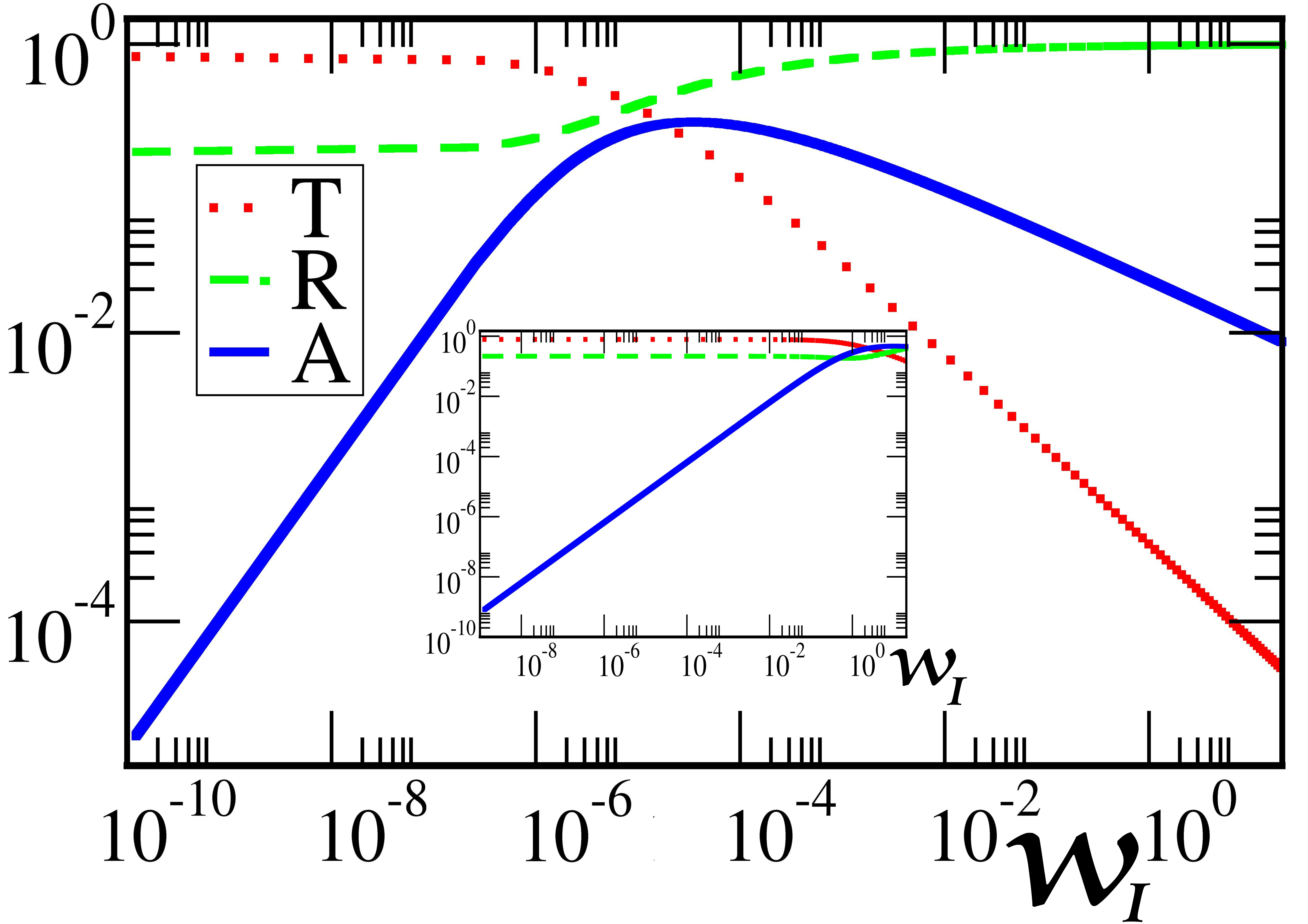
Figure 3: (Color online) Transport characteristics for the model of a non-linear $\delta-$like defect embedded in a Bragg grating. The theoretical results of Eq. (7) shown here, reproduce nicely the features of the simulations reported in Fig 2. In the inset we report, for comparison, $\mathcal{A},\mathcal{T}$ and $\mathcal{R}$ for a single non-linear layer. We assume normal incidence at $\omega=0.7\approx\omega_{r}$.

Fig. 3 demonstrates the effect of $\mathcal{W}_{I}$ on a resonant localized mode for the case of symmetrically placed Bragg gratings on the left and right side of a $\delta-$like defect. The alternate layers at the Bragg gratings have permittivity $\epsilon_{1}=4$ and $\epsilon_{2}=9$ while the permittivity of the defect layer is $\epsilon=1.5$. The transport characteristics of the gratings $t_{L}=t_{R}$ and $r_{L}=r_{R}$ have been calculated numerically and used as inputs in Eqs. (7). We find (see Fig. 3) that the overall behavior of $\mathcal{T}$, $\mathcal{R}$ and $\mathcal{A}$ is similar to the one observed in the simulations of Fig. 2.

For comparison, we also report (inset of Fig. 3) the behavior of $\mathcal{T},\mathcal{A}$ and $\mathcal{R}$, for a single non-linear layer (without any Bragg gratings), vs. the incident intensity $\mathcal{W}_{I}$. They are calculated analytically using the continuity of the field and the discontinuity of its derivative at the position of the $\delta-$defect. Specifically, $\mathcal{T}=\frac{4}{(k\epsilon_{0})^{2}+(2+k\epsilon_{0}\gamma|E_{f}^{+}|^{2})^{2}};\,\mathcal{R}=(k\epsilon_{0})^{2}(1+\gamma^{2}|E_{f}^{+}|^{4})\mathcal{T}/4$ and $A=k\epsilon_{0}\gamma|E_{f}^{+}|^{2}\mathcal{T}$. We find that for moderate $\mathcal{W}_{I}$-values the single non-linear layer is mainly absorptive (inset of Fig. 3) while the structure of Fig. 1 is mainly reflecting the incident light back to space (main panel of Fig. 3).

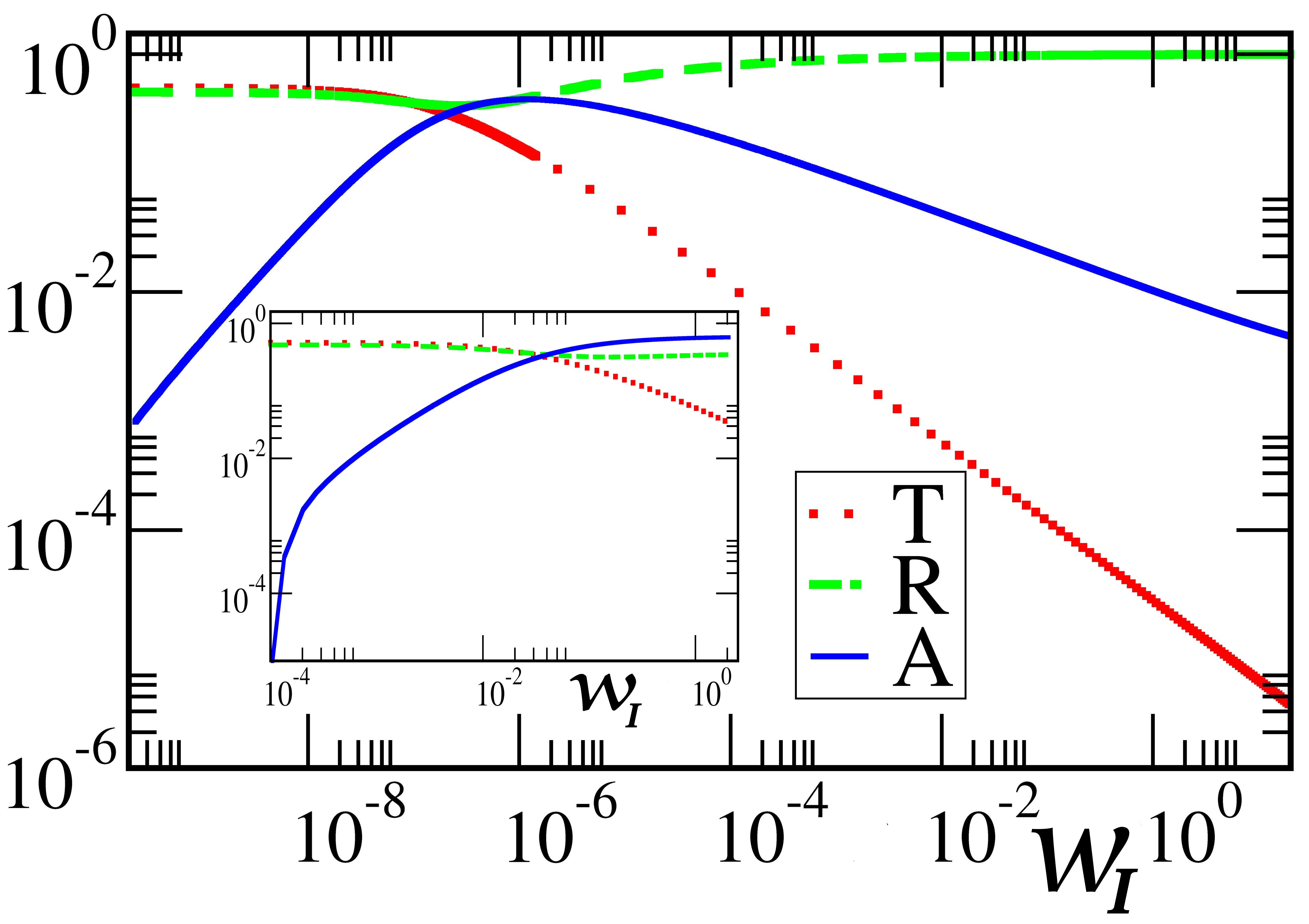
Figure 4: (Color online) Simulations for the structure of Fig. 1 for oblique incidence at $\omega=8.95\approx\omega_{r}$. The parameters of the grating are indicated at the text while the incident angle is $\phi=6^{o}$. We find that for moderate values of the incident light intensity $\mathcal{W}_{I}$, the transmittance and absorption are suppressed and the system is reflective i.e. $\mathcal{R}=1$. In the inset we report for comparison (and for the same range of $\mathcal{W}_{I}$-values) the $\mathcal{A},\mathcal{T},\mathcal{R}$ values for the case of a single non-linear layer. This system mainly absorbs the incident energy.

We have also investigated the efficiency of the proposed limiter in the case of oblique incidence MRVK13 . A representative example in the case of an incident angle $\phi=6^{o}$ is shown in Fig. 4. The Bragg grating considered in this example consists of two layers with permittivities $\epsilon_{1}=9$, $\epsilon_{2}=16$ while the non-linear impurity has permittivity $\epsilon=16$. We find again that as the incident light intensity $\mathcal{W}_{I}$ takes moderate values, the transmittance and the absorption are suppressed and the structure becomes reflective i.e. $\mathcal{R}\approx 1$. This behavior has to be contrasted with the one found for the single non-linear layer where for moderate $\mathcal{W}_{I}$-values the dominant mechanism is absorption, see the inset of Fig. 4.

The effectiveness of the structure of Fig. 1 to act as a self-protecting power limiter for any incident angle calls for a generic argument for its explanation. The following heuristic argument, provides some understanding of the mechanism underlying our structure. First we recall that the defect results in the creation of a resonance mode which is localized around the impurity layer at $z=0$ and decays away from its localization center with an envelope profile $E_{\mathrm{r}}(z)\sim\exp(-\alpha|z|)$. An incoming (say from the left) wave that carries an incident energy flux $\mathcal{S}$ can resonate via this mode as long as the loss coefficient is $\gamma\leq\gamma^{*}\sim\mathcal{S}/{\cal W}_{0}\sim\exp(-2\alpha L)$ (${\cal W}_{0}\sim|E_{\mathrm{r}}(z=0)|^{2}\sim\exp(2\alpha L)$ is the mode intensity at $z=0$ note2 ). In other words the energy that is absorbed from the non-linear lossy layer via the resonant mode cannot be more than the incoming energy. Therefore for any $\gamma>\gamma^{*}$ the resonant mode will not be sustained and thus the transmission will be $\mathcal{T}=0$.

We proceed in our argument by noticing that the resonant mode is located at the band-gap of the Bragg grating and therefore it can be written as a superposition of two evanescent modes, one growing and another one decaying i.e. $E_{\mathrm{r}}(z)\sim\psi_{+}(z)+\psi_{-}(z)$, where $\psi_{-}\sim\alpha_{-}\exp(-z)$ and $\psi_{+}\sim\alpha_{+}\exp(z)$. Let us assume that $\alpha_{+}\sim\mathcal{O}(1)$ note3 . Then the field at the outer boundary of the left grating at $z=-L$ is $E_{\mathrm{r}}(z=-L)=\alpha_{+}\exp(-L)+\alpha_{-}\exp(L)\sim\alpha_{-}\exp(L)$. At the same time due to continuity at the boundary we expect that the resonance wavefunction must be equal to the incoming field which we assume to take some constant value i.e. $\alpha_{-}\exp(L)\sim\mathcal{O}(1)$. This can only happen if $\alpha_{-}\rightarrow 0$. Finally we recall that the incoming energy flux is given by the Poynting vector $\mathcal{S}$ which in the case of evanescent modes is $S\sim\psi_{+}\psi_{-}=\alpha_{+}\alpha_{-}\rightarrow 0$ Ilya . Therefore there will be no net flux towards the structure and thus $\mathcal{A}=0$. Since $\mathcal{T}=0$ and $\mathcal{A}=0$ we conclude that almost all the incident energy is reflected back i.e. $\mathcal{R}\rightarrow 1$.

In conclusion, we have examined the scattering problem for a periodic layered structure with an embedded nonlinear defect layer. We presume that the absorption coefficient of the defect layer increases with the light intensity, which is normally the case. We have shown that such a layered structure acts as a self-protecting power limiter. Specifically, at low intensity of the incident light, the entire stack is highly transmissive. When the light intensity increases, the stack transmission decreases. Initially, the fraction of the input power absorbed by the lossy nonlinear layer also increases with the incident light intensity. But when the input power exceeds a certain level, the stack becomes highly reflective within a broad frequency range and regardless of the angle of incidence. In other words, the excessive radiation will be reflected back to space, rather than being absorbed by the limiter, which can prevent overheating and destruction of the limiter. A simplest realization of such a self-protected (reflective) power limiter is provided by a lossy non-linear layer sandwiched between two Bragg gratings. A shortcoming of such a design is that although the high intensity radiation will be reflected back to space within a broad frequency range, the low-intensity transmittance only occurs within a narrow frequency band corresponding to the frequency of the localized mode. This problem can be addressed by using a more sophisticated, structured defect layer, as well as a chain of several coupled nonlinear defects. The latter possibilities are currently under investigation MRVK13 .

Acknowledgments - This work is sponsored by the Air Force Research Laboratory (AFRL/RYDP) through the AMMTIAC contract with Alion Science and Technology, and by the Air Force Office of Scientific Research LRIR09RY04COR and FA 9550-10-1-0433.

References

- (1) B. E. A. Saleh and M. C. Teich, Fundamentals of Photonics (Wiley, New York, 1991).
- (2) T. Ohtsuki, J. Lightwave Technol. 15, 452 (1997)
- (3) N. S. Patel, K. L. Hall and K. A. Rauschenbach, Appl. Opt. 37, 2831 (1998)
- (4) L. W. Tutt, T. F. Boggess, Prog. Quant. Electr. 17, 299 (1993); A. E. Siegman, Appl. Opt. 1, 739 (1962); J. E. Geusic, S. Singh, D. W. Tipping, and T. C. Rich, Phys. Rev. Lett. 19, 1126 (1969).
- (5) Y. Zeng, X. Chen, W. Lu, J. Appl. Phys. 99, 123107 (2006); M. Scalora, J. P. Bowling, C. M. Bowden, M. J. Bloemer, Phys. Rev. Lett. 73, 1368 (1994)
- (6) S. Husaini, et al., Appl. Phys. Lett. 102, 191112 (2013); S. Pawar, et al., J. Nonlin. Opt. Phys. & Mat. 21, 1250017 (2012).
- (7) Macleod H. A. 2001 Thin-Film Optical Filters (Bristol and Philadelphia: Institute of Physics Publishing)
- (8) The quantities are the same for a right incident wave as well, since our structure is reciprocal.
- (9) In all numerical simulations in Figs. 2-4 we use units such that .
- (10) E. Makri, H. Ramezani, I. Vitebskiy, T. Kottos, in preparation (2013).
- (11) We assume the incident wave has amplitude and that due to continuity of the wavefunction at the boundary
- (12) A similar argument can be used for .
- (13) A. Figotin and I. Vitebskiy, Waves in Random and Complex Media 16, 293 (2006).