Faithful tropicalization of the Grassmannian of planes

Abstract.

We show that the tropical projective Grassmannian of planes is homeomorphic to a closed subset of the analytic Grassmannian in Berkovich’s sense by constructing a continuous section to the tropicalization map. Our main tool is an explicit description of the algebraic coordinate rings of the toric strata of the Grassmannian. We determine the fibers of the tropicalization map and compute the initial degenerations of all the toric strata. As a consequence, we prove that the tropical multiplicities of all points in the tropical projective Grassmannian are equal to one. Finally, we determine a piecewise linear structure on the image of our section that corresponds to the polyhedral structure on the tropical projective Grassmannian.

1. Introduction

In this paper, we investigate the tropical Grassmannian of planes in $n$-space from the point of view of non-Archimedean analytic geometry. The deep relations between tropical and non-Archimedean analytic geometry have been studied by several authors, including Einsiedler, Kapranov and Lind [12], Gubler [16, 17] and Payne [25]. Analytic spaces in this context are mostly Berkovich analytic spaces, where, roughly speaking, points can locally be described by certain seminorms. Spaces of seminorms or valuations have been present in tropical geometry from its very beginnings by the work of Bieri and Groves [5]. Recently, such spaces have been used by Manon to investigate representations of reductive groups [21, 22].

Of particular interest for the present paper is the recent work by Baker, Payne and Rabinoff [1], which contains a detailed study of the connections between tropicalizations and skeleta of Berkovich analytic curves. Our study of the Grassmannian of planes provides higher-dimensional results in the same direction.

The tropicalization map on an analytic closed subvariety of a toric variety is continuous and surjective, and it strongly depends on a choice of coordinates of $X$. Work of Payne shows that the Berkovich space $X^{\operatorname{an}}$ associated to a closed subvariety $X$ of a toric variety is homeomorphic to the projective limit of all tropicalizations of $X$ [25, Theorem 4.2].

Berkovich introduced skeleta of analytic spaces, roughly speaking, as polyhedral subsets that are deformation retracts of the whole space [3]. For concrete examples, we refer to Section 2.1. These piecewise linear substructures of analytic spaces were used in [3, 4] to prove local contractibility of smooth analytic spaces.

If $X$ is a curve, the corresponding Berkovich space $X^{\operatorname{an}}$ can be endowed with a polyhedral structure locally modeled on an $\mathbb{R}$-tree. The complement of its set of leaves carries a canonical metric. As Baker, Payne and Rabinoff have shown, every finite subgraph $\Gamma$ of this complement maps isometrically to a suitable tropicalization of $X$ [1, Theorem 6.20], where the metric on this tropicalization is given locally by lattice lengths. We say that this tropicalization represents $\Gamma$ faithfully. When all tropical multiplicities equal one, any compact connected subset of a tropicalization is the isometric image of a suitable subgraph of $X^{\operatorname{an}}$ [1, Theorem 6.24]. The proofs of these two statements rely on deep results concerning the structure theory of analytic curves and their semistable reduction theory. Some of them were developed by Thuillier in the context of potential theory on curves [31].

The former results can be seen as a comparison between two polyhedral approximations of analytic curves. The first one is given by all tropicalizations (which approximate the analytic space by Payne’s theorem cited above), whereas the second one comes from skeleta of semistable models. An interesting challenge is to look for a comparison of these two different polyhedral approximations for higher dimensional varieties. Two major difficulties arise in this case. First, there is no polyhedral description of the full Berkovich space generalizing the $\mathbb{R}$-tree description for curves. And second, there are no semistable models available in general. Also, in higher dimensions, skeleta are endowed with piecewise linear structures and not with canonical metrics. Still, we can ask the following natural question. Let $X$ be a closed subvariety of a toric variety. Is there a continuous map from the tropicalization of $X$ to $X^{\operatorname{an}}$ that is a section to the tropicalization map? If the answer is yes, we call such a tropicalization faithful.

In this paper we show that the tropicalization of the Grassmannian of planes $\operatorname{Gr}(2,n)$ induced by the Plücker embedding (3.1) into $\mathbb{P}_{K}^{\binom{n}{2}-1}$ satisfies this property, where $K$ is a complete non-Archimedean field. Let us describe our main results in more detail. Via the Plücker map, we embed $\operatorname{Gr}(2,n)^{\operatorname{an}}$ into the analytified projective space $(\mathbb{P}_{K}^{\binom{n}{2}-1})^{\operatorname{an}}$. The composition with the coordinatewise logarithmic absolute value gives a continuous map called tropicalization, i.e., $\operatorname{trop}\colon\operatorname{Gr}(2,n)^{\operatorname{an}}\rightarrow(\overline{\mathbb{R}}^{\binom{n}{2}}\smallsetminus\{(-\infty,\ldots,-\infty)\})/\mathbb{R}\!\cdot\!\mathbf{1}$, where $\mathbf{1}$ is the all-ones vector. Here, we put $\overline{\mathbb{R}}=\mathbb{R}\cup\{-\infty\}$ and set the logarithmic absolute value of zero to be $-\infty$. The image of $\operatorname{trop}$ is the tropical Grassmannian $\mathcal{T}\!\operatorname{Gr}(2,n)$. By $\operatorname{Gr}_{0}(2,n)$ we denote the Zariski open subset of the Grassmannian mapping to the complement of the coordinate hyperplanes under the Plücker embedding. Its tropicalization ${\mathcal{T}\!\operatorname{Gr}_{0}}(2,n):=\operatorname{trop}(\operatorname{Gr}_{0}(2,n)^{\operatorname{an}})\subset\mathbb{R}^{\binom{n}{2}}/\mathbb{R}\!\cdot\!\mathbf{1}$ was introduced and studied by Speyer and Sturmfels [27]. Investigating the full space $\mathcal{T}\!\operatorname{Gr}(2,n)$ introduces technical difficulties involving the boundary $\mathcal{T}\!\operatorname{Gr}(2,n)\smallsetminus{\mathcal{T}\!\operatorname{Gr}_{0}}(2,n)$, which we explain in Section 4.

The main result in this paper can be phrased as follows:

Theorem 1.1.

There exists a continuous section $\sigma\colon\mathcal{T}\!\operatorname{Gr}(2,n)\to\operatorname{Gr}(2,n)^{\operatorname{an}}$ to the tropicalization map $\operatorname{trop}\colon\operatorname{Gr}(2,n)^{\operatorname{an}}\to\mathcal{T}\!\operatorname{Gr}(2,n)$. Hence, the tropical Grassmannian $\mathcal{T}\!\operatorname{Gr}(2,n)$ is homeomorphic to a closed subset of the Berkovich analytic space $\operatorname{Gr}(2,n)^{\operatorname{an}}$.

This section is constructed locally and it is defined by skeleton maps on affine spaces, after a suitable choice of local coordinates. Our construction relies on the interpretation of the tropical Grassmannian as a compactification of the space of phylogenetic trees, extending earlier work of Speyer and Sturmfels [27]. To be more precise, we define $\sigma$ on a covering of $\mathcal{T}\!\operatorname{Gr}(2,n)$ by polyhedral cones which we call $\{\mathscr{C}^{(ij)}_{T,J}\}_{ij,T,J}$. Each cone consists of those points in $\mathcal{T}\!\operatorname{Gr}(2,n)$ associated to the combinatorial type of a tree $T$ whose only non-finite coordinates involving either $i$ or $j$ are those contained in $J$. The pair $ij$ of distinct indices lies outside $J$. For every such cone $\mathscr{C}^{(ij)}_{T,J}$, we construct an algebraically independent subset $I$ of the Plücker coordinates of cardinality $2(n-2)$ such that the corresponding affine space $\mathbb{A}^{I}_{K}$ intersects the Grassmannian in a Zariski open subvariety. The Berkovich skeleton of $(\mathbb{A}^{I}_{K})^{\operatorname{an}}$ can be identified with $\overline{\mathbb{R}}^{2(n-2)}$. The natural inclusion of the skeleton $\overline{\mathbb{R}}^{2(n-2)}$ into $(\mathbb{A}^{I}_{K})^{\operatorname{an}}$ induces the section $\sigma$ on $\mathscr{C}^{(ij)}_{T,J}$. In order to prove that this map is well-defined, we check by direct computation that for each $x\in\mathcal{T}\!\operatorname{Gr}(2,n)$, the point $\sigma(x)$ is the unique maximal element in the fiber $\operatorname{trop}^{-1}(x)$ with respect to evaluation on rational functions (Lemma 4.17). We show the continuity of $\sigma$ in Theorem 4.19.

The Plücker embedding induces a stratification of $\operatorname{Gr}(2,n)$ by subvarieties of tori. For every subset $J$ of the Plücker coordinates, we denote by $\operatorname{Gr}_{J}(2,n)$ the subvariety of $\operatorname{Gr}(2,n)$ where precisely the Plücker coordinates in $J$ vanish. For example, when $J$ is empty, we recover the open subset $\operatorname{Gr}_{0}(2,n)$. In Lemma 5.3, we use the local coordinate systems $I$ mentioned above to describe the coordinate ring of $\operatorname{Gr}_{J}(2,n)$. This step is crucial to characterize the fiber of $\operatorname{trop}$ over a point $x$ in $\mathcal{T}\!\operatorname{Gr}(2,n)$ as the Berkovich spectrum of an affinoid algebra. This is the content of Proposition 5.6 and Theorem 5.8. Corollary 5.9 shows that each of these affinoid algebras has a unique Shilov boundary point, which is precisely $\sigma(x)$. This gives a conceptual explanation for the fact that $\sigma(x)$ is maximal in the fiber $\operatorname{trop}^{-1}(x)$.

In Section 6 we focus our attention on piecewise linear structures. In Lemma 6.2, we use the local coordinates $I$ to compute the initial degenerations of each subvariety $\operatorname{Gr}_{J}(2,n)$. Theorem 6.4 states that these degenerations are integral schemes, and that they coincide with the reductions of the affinoid algebras given by the fibers of tropicalizations. Each stratum $\mathcal{T}\!\operatorname{Gr}_{J}(2,n)$ is endowed with the induced Gröbner fan structure associated to its defining ideal. In Corollary 6.5, we show that the tropical multiplicity of every point in the tropical Grassmannian, evaluated in the corresponding stratum $\operatorname{Gr}_{J}(2,n)$, is equal to one. This provides an example of the general comparison theorem [1, Proposition 4.24] as well as a test case for a higher-dimensional version of [1, Theorem 6.23].

On the analytic side, Corollary 6.8 states that the image of the section $\sigma$ is a skeleton in the sense of Ducros [11]. Note that we do not consider skeleta of semistable models of the Grassmannian, although it seems likely that the image of $\sigma$ can be identified with a skeleton of such a model. Therefore there is, a priori, no natural piecewise linear structure on the image of $\sigma$. However, the properties of $\sigma$ allow us to define a natural piecewise linear structure on this set. We do so at the end of Section 6.

The rest of the paper is organized as follows. In Section 2, we recall basic facts on tropical and analytic varieties. In Section 3, we describe the combinatorics and topological structure of the tropical Grassmannian of $2$-planes in $n$-space, following the seminal work of Speyer and Sturmfels [27]. Section 4 contains the proof of Theorem 1.1. In Section 5 we give an explicit description of the fibers of the tropicalization map in the language of affinoid domains. Section 6 deals with piecewise linear structures. In Section 7 we discuss how the construction of the section $\sigma$ leads to an embedding of the quotient of the tropical fan ${\mathcal{T}\!\operatorname{Gr}_{0}}(2,n)$ by its $(n-1)$-dimensional lineality space into a quotient of $\operatorname{Gr}(2,n)^{\operatorname{an}}$ by a torus action. This application is motivated by a question of Sturmfels to the third author.

We hope that the exhaustive study of the tropical and analytic Grassmannian carried out in this paper will provide a helpful guideline to obtain further general results along the lines of [1] for higher-dimensional varieties. Finally, we believe that the local coordinates introduced to explicitly construct our section will be a useful tool to further investigate the algebraic Grassmannian.

2. Analytification and tropicalization

Throughout this paper, we let $K$ be a field which is complete with respect to a non-Archimedean valuation $\nu\colon K^{\ast}=K\smallsetminus\{0\}\to\mathbb{R}$. This valuation induces an absolute value $|\,\mathord{\cdot}\,|=\exp(-\nu(\mathord{\cdot}))$ on $K$. Note that we allow $K$ to be an arbitrary field endowed with the trivial absolute value. Other examples include non-Archimedean local fields such as $\mathbb{Q}_{p}$, the completion $\mathbb{C}_{p}$ of the algebraic closure of $\mathbb{Q}_{p}$, the field $\mathbb{C}(\!(t)\!)$ of formal power series, and the field $\mathbb{C}\{\!\{t\}\!\}$ of Puiseux series.

In order to study tropicalizations of projective varieties, it is convenient to extend the field $\mathbb{R}$ as well as the valuation $\nu$ from $K^{\ast}$ to $K$, setting $\nu(0)=\infty$. Let $\overline{\mathbb{R}}=\mathbb{R}\cup\{-\infty\}$ be the extended field of real numbers. It is an additive monoid, and its topology extends the Euclidean topology on $\mathbb{R}$. The half-open intervals $[-\infty,a)$ for $a\in\mathbb{R}$ give a basis of open neighborhoods of $-\infty$.

In what follows, we use multi-index notation. More precisely, given $x=(x_{1},\ldots,x_{n})\in K^{n}$ and $\alpha\in\mathbb{Z}^{n}$, we write $x^{\alpha}=\prod_{i=1}^{n}x_{i}^{\alpha_{i}}$ and $|\alpha|=\alpha_{1}+\ldots+\alpha_{n}$.

2.1. Analytic spaces

Let us recall some basic facts about Berkovich analytic spaces. The analytification functor associates to every $K$-scheme of finite type an analytic space over $K$ [2, Sections 3.4 and 3.5]. If $X=\operatorname{\operatorname{Spec}}B$ is an affine $K$-scheme of finite type, then $X^{\operatorname{an}}$ can be identified with the set of all multiplicative seminorms on $B$ extending the absolute value on $K$ [2, Remark 3.4.2]. Here, a multiplicative seminorm is a map of multiplicative monoids $\|\mathord{\cdot}\|\colon B\to\mathbb{R}_{\geqslant 0}$ sending zero to zero and satisfying the non-Archimedean triangle inequality, i.e., $\|f+g\|\leqslant\max\{\|f\|,\|g\|\}$ for all $f,g\in B$. The space $X^{\operatorname{an}}$ has a natural topology, namely, the coarsest one such that all evaluation maps $\operatorname{ev}_{f}\colon\|\mathord{\cdot}\|\mapsto\|f\|$ with $f$ in $B$ are continuous. When $X$ is a general $K$-scheme of finite type, $X^{\operatorname{an}}$ is constructed by gluing the analytifications on any open affine cover [2, Proof of Theorem 3.4.1 (3)].

As we mentioned in the Introduction, a skeleton of an analytic space is a polyhedral subset satisfying a finiteness condition. Rather than giving the precise definition, we focus on the following example, which we thoroughly use in the sequel.

Example 2.1 (Affine $n$-space).

The analytic affine $n$-space $(\mathbb{A}_{K}^{n})^{\operatorname{an}}$ consists of all multiplicative seminorms on $K[x_{1},\ldots,x_{n}]$ extending the absolute value of $K$. Given any point $\rho\in\overline{\mathbb{R}}^{n}$, we define a multiplicative seminorm $\delta(\rho)$ on $K[x_{1},\ldots,x_{n}]$ as follows:

$$\delta(\rho)\colon K[x_{1},\ldots,x_{n}]\longrightarrow\mathbb{R}_{\geqslant 0}\qquad\delta(\rho)(\sum_{\alpha}c_{\alpha}{x}^{\alpha})=\max_{\alpha}\{|c_{\alpha}|\exp(\sum_{i=1}^{n}{\rho_{i}\alpha_{i}})\}.$$

Here, we put $\exp(-\infty)=0$. The map $\delta$ is continuous and injective. The image of $\delta$ is the skeleton of the analytic affine space, so we call $\delta$ the skeleton map. Note that $\delta$ and the corresponding skeleton depend on the choice of affine coordinates on $\mathbb{A}^{n}_{K}$.

The restriction of $\delta$ to $\mathbb{R}^{n}$ is a continuous map $\delta\colon\mathbb{R}^{n}\to(\mathbb{G}_{m}^{n})^{\operatorname{an}}$. The image of $\delta$ is called the skeleton of the split torus $(\mathbb{G}_{m}^{n})^{\operatorname{an}}$. It is a deformation retract of $(\mathbb{G}_{m}^{n})^{\operatorname{an}}$. $\diamond$

Example 2.2 (Projective $n$-space).

The analytic projective space $(\mathbb{P}^{n}_{K})^{\operatorname{an}}$ can be obtained by gluing the analytifications of the standard open covering of $\mathbb{P}^{n}_{K}$ by $n+1$ copies of $\mathbb{A}_{K}^{n}$. It can also be described with the following equivalence relation of $(\mathbb{A}_{K}^{n+1})^{\operatorname{an}}\smallsetminus\{0\}$. Two elements $\|\mathord{\cdot}\|_{1}$ and $\|\mathord{\cdot}\|_{2}$ in $(\mathbb{A}_{K}^{n+1})^{\operatorname{an}}\smallsetminus\{0\}$ are equivalent if for every positive integer $d$ there exists a constant $C=C(d)\in\mathbb{R}_{>0}$ such that $\|f\|_{1}=C^{d}\|f\|_{2}$ for any homogeneous polynomial $f$ in $K[x_{0},\ldots,x_{n}]$ of degree $d$. The topological space $(\mathbb{P}^{n}_{K})^{\operatorname{an}}$ can be identified with the set of equivalence classes in $(\mathbb{A}_{K}^{n+1})^{\operatorname{an}}\smallsetminus\{0\}$, equipped with the quotient topology. $\diamond$

2.2. Tropicalizations

We now introduce some notation for tropicalizations. For every $K$-split torus $\mathbb{G}_{m}^{n}$ and every basis $\{\chi_{1},\ldots,\chi_{n}\}$ of its character lattice $\Lambda$, we define a tropicalization map

(2.1) $$\operatorname{trop}\colon(\mathbb{G}_{m}^{n})^{\operatorname{an}}\longrightarrow\mathbb{R}^{n}\qquad\gamma\longmapsto(\log|\chi_{1}(\gamma)|,\ldots,\log|\chi_{n}(\gamma)|).$$

Definition 2.3.

If $X$ is a closed subscheme of $\mathbb{G}_{m}^{n}$, the tropical variety $\mathcal{T}X$ is the image of $X^{\operatorname{an}}$ under the tropicalization map.

These notions extend the classical tropicalizations of subvarieties of tori by valuation maps [30]. Indeed, let $L|K$ be an algebraically closed, complete non-Archimedean valued field with nontrivial valuation extending the valuation on $K$. Every closed point $x$ in $X(L)$ induces a seminorm $\gamma_{x}$ in $X^{\operatorname{an}}$, sending $f\mapsto|f(x)|$, where $f\in K[X]$. The restriction of the tropicalization map (2.1) to $X(L)$ is the negative of the coordinatewise valuation map on the split torus over $L$. By the Fundamental theorem of tropical geometry, the closure of $\operatorname{trop}(X(L))$ coincides with $\mathcal{T}X$ (see [18, Proposition 3.8] and [10, 12, 26]).

In order to define tropicalizations of projective varieties, we first need to describe tropical projective space. We write $\mathbf{1}$ for $(1,1,\ldots,1)$ and $-\mathbf{\infty}\!\cdot\!\mathbf{1}$ for $(-\infty,-\infty,\ldots,-\infty)$.

Definition 2.4.

The tropical projective space is the topological space

$$\mathbb{T}\mathbb{P}^{n}=(\overline{\mathbb{R}}^{n+1}\smallsetminus\{-\mathbf{\infty}\!\cdot\!\mathbf{1}\})/\mathbb{R}\!\cdot\!\mathbf{1}\text{,}$$

endowed with the quotient topology.

Let $\{x_{0},\ldots,x_{n}\}$ be the projective coordinates on $\mathbb{P}^{n}_{K}$. Using Example 2.2, we define the associated tropicalization map on $(\mathbb{P}^{n}_{K})^{\operatorname{an}}$:

(2.2) $$\operatorname{trop}\colon(\mathbb{P}^{n}_{K})^{\operatorname{an}}\longrightarrow\mathbb{T}\mathbb{P}^{n}\qquad[\gamma]\longmapsto(\log\gamma(x_{0}),\ldots,\log\gamma(x_{n}))+\mathbb{R}\!\cdot\!\mathbf{1}\text{.}$$

Here, $[\gamma]$ denotes the equivalence class of a nonzero multiplicative seminorm $\gamma$ on $K[X_{0},\ldots,X_{n}]$. By convention, we set $\log 0=-\infty$.

Definition 2.5.

Given a projective variety $X\subset\mathbb{P}^{n}_{K}$, we define its tropicalization $\mathcal{T}X$ as the image of $X^{\operatorname{an}}$ in $\mathbb{T}\mathbb{P}^{n}$ under the tropicalization map (2.2).

3. The tropical Grassmannian $\mathcal{T}\!\operatorname{Gr}(2,n)$

Our object of study is the Grassmannian $\operatorname{Gr}(2,n)$ of $2$-planes in $n$-space. We view this variety inside projective space via the Plücker map, which we now recall. We write $[n]=\{1,\ldots,n\}$ and $ij\in\binom{[n]}{2}$ for a subset $\{i,j\}\subset[n]$ of size $2$. The Plücker map is given by the formula

$$\tilde{\varphi}\colon\mathbb{A}_{K}^{2\times n}\dashrightarrow\mathbb{P}^{\binom{n}{2}-1}_{K}\qquad\tilde{\varphi}(X)=\big{(}\det(X^{(ij)})\big{)}_{i<j}\text{,}$$

where $X^{(ij)}$ denotes the submatrix of $X$ obtained by choosing the $i$th and $j$th columns of $X$. The locus of definition of $\tilde{\varphi}$ is the open set of matrices of rank two, which we identify with the set of $2$-planes in $n$-space. This map induced the Plücker embedding

(3.1) $$\varphi\colon\operatorname{Gr}(2,n)\to\mathbb{P}^{\binom{n}{2}}_{K}.$$

We set $p_{ij}:=\det(X^{(ij)})$. As it is customary, for each pair $\{i,j\}$, we choose only one projective coordinate among $p_{ij}$ and $p_{ji}$. They are related by the identity $p_{ij}=-p_{ji}$. Abusing notation, we consider each index as an unordered pair.

The Plücker ideal $I_{2,n}$ is the homogeneous prime ideal in the polynomial ring $K[p_{ij}:ij\in\binom{[n]}{2}]$ of all algebraic relations among the $2\times 2$-minors of a generic $2\times n$-matrix $X$. This ideal is generated by quadrics with coefficients in $\mathbb{Z}$ and it admits a quadratic Gröbner basis [28, Theorem 3.1.7]. A particularly nice system of generators for the ideal $I_{2,n}$ is given by the three-term Plücker relations

(3.2) $$p_{ij}p_{kl}-p_{ik}p_{jl}+p_{il}p_{jk}=0\qquad\text{ for }ijkl\in\binom{[n]}{4}.$$

We cover the variety $\operatorname{Gr}(2,n)$ by $\binom{n}{2}$ big open cells, all of which are isomorphic to $\mathbb{A}_{K}^{2(n-2)}$:

(3.3) $$U_{ij}=\varphi^{-1}(\{p_{ij}\neq 0\})\qquad\text{ for }ij\in\binom{[n]}{2}.$$

The intersection of all $U_{ij}$ is the open subvariety

$$\operatorname{Gr}_{0}(2,n):=\varphi^{-1}(\mathbb{G}_{m}^{\binom{n}{2}}/\mathbb{G}_{m})\text{,}$$

where $\mathbb{G}_{m}$ is embedded diagonally.

We tropicalize the Grassmannian $\operatorname{Gr}(2,n)$ and the open subvariety $\operatorname{Gr}_{0}(2,n)$ with respect to its Plücker embedding by means of the tropicalization map (2.2). Similarly, for each pair $ij$, we define $\mathcal{T}U_{ij}$ as the image of $U_{ij}^{\operatorname{an}}\subset\operatorname{Gr}(2,n)$ under the same map. In particular, we obtain

(3.4) $$\mathcal{T}U_{ij}=\{x\in\mathcal{T}\!\operatorname{Gr}(2,n):x_{ij}\neq-\infty\}.$$

To analyze these tropical varieties in more detail, we consider the affine cone over the Grassmannian $\operatorname{Gr}_{0}(2,n)_{\operatorname{\operatorname{aff}}}=\operatorname{\operatorname{Spec}}(K[p_{ij}^{\pm}:ij\in\binom{[n]}{2}]/I_{2,n})$ in $\mathbb{G}_{m}^{\binom{n}{2}}$. The resulting tropical Grassmannian ${\mathcal{T}\!\operatorname{Gr}_{0}}(2,n)_{\operatorname{\operatorname{aff}}}$ of $2$-planes in $n$-space is a polyhedral fan in $\mathbb{R}^{\binom{n}{2}}$ of pure dimension $2n-3$, all of whose cones contain the line spanned by the all-ones vector $\mathbf{1}$. It is a closed subfan of the Gröbner fan of $I_{2,n}$ [6, Section 2]. The quotient of ${\mathcal{T}\!\operatorname{Gr}_{0}}(2,n)_{\operatorname{\operatorname{aff}}}$ by $\mathbb{R}\!\cdot\!\mathbf{1}$ equals ${\mathcal{T}\!\operatorname{Gr}_{0}}(2,n)\subset\mathbb{T}\mathbb{P}^{\binom{n}{2}-1}$.

In [27], Speyer and Sturmfels identified the space ${\mathcal{T}\!\operatorname{Gr}_{0}}(2,n)$ with the space of phylogenetic trees, the definition of which we recall now. A phylogenetic tree on $n$ leaves is a real weighted tree $(T,\omega)$. Here, $T$ is a finite connected graph with no cycles and with no degree-two vertices, together with a labeling of its leaves in bijection with $[n]$. All the trees in this paper will be labeled. We define the set of inner edges of $T$ as those that do not end in a leaf of $T$. The weight function $\omega\colon E(T)\to\mathbb{R}$ is defined on the set of edges of $T$. We impose the condition that the weight of every inner edge of $T$ is nonnegative. The tree $T$ is called the combinatorial type of the phylogenetic tree $(T,\omega)$.

Given a phylogenetic tree $(T,\omega)$, we construct a distance function on $[n]$ as follows. For any pair of leaves $i,j$ in $T$, we let $x_{ij}$ be the sum of the weights $\omega(e)$ of all edges $e$ in the path from $i$ to $j$ in $T$. Note that this number could be negative. Tree-distance functions are characterized by the four-point condition [8, Theorem 1].

Theorem 3.1 (Four-point condition).

A point $x\in\mathbb{R}^{\binom{n}{2}}$ is the distance function associated to a phylogenetic tree on $n$ leaves if and only if for all pairwise distinct indices $i,j,k,l\in[n]$, the maximum among

(3.5) $$x_{ij}+x_{kl},\quad x_{ik}+x_{jl},\quad x_{il}+x_{jk}$$

is attained at least twice.

As we discussed earlier, any $K$-point $x$ in the Grassmannian $\operatorname{Gr}(2,n)$ satisfies the Plücker relations (3.2). It is immediate to check that $\operatorname{trop}(x)$ satisfies Theorem 3.1.

Assuming that $i,j,k$ and $l$ are distinct, we can look at the subtree of $T$ spanned by these four leaves. Such a subtree is called a quartet. It is a well-known fact that the list of quartets on a phylogenetic tree characterizes its combinatorial type [19, §5.4.2]. There are exactly four combinatorial types for quartet trees. These types are distinguished by the pairs of indices attaining the maximum in (3.5).

The type of a quartet tree is also determined by its cherries, which are defined as follows.

Definition 3.2.

Let $T$ be a tree. A cherry of $T$ is a pair of leaves $\{i,j\}$ in the tree $T$ with the property that they are both adjacent to the same node in $T$. Equivalently, the induced path from $i$ to $j$ in $T$ has only one internal node.

For example, the unique cherries in the caterpillar tree on $n$ leaves depicted on the left of Figure 1 are $\{i,s_{1}\}$ and $\{j,s_{n-2}\}$. Notice that for trivalent trees (i.e., where all its internal nodes have degree three) our definition of cherry coincides with the standard one [24, Chapter 2.4]. We can determine the cherries of a quartet by (3.5). Indeed, the pairing of the indices $i,j,k,l$ realizing the minimal value in (3.5) gives the two cherries of the quartet $\{i,j,k,l\}$. If all three numbers in (3.5) agree, the quartet has no internal edge. We call such a tree the star tree on four leaves.

From [27, Theorem 3.4] we know that the open cell ${\mathcal{T}\!\operatorname{Gr}_{0}}(2,n)$ equipped with its Gröbner fan structure is the space of phylogenetic trees. The relative interior of each cone in this fan is associated to one combinatorial type of a phylogenetic tree. We make this correspondence explicit by writing $\mathscr{C}_{T}$ for the cone whose relative interior is associated to the tree $T$. Each tree has exactly $n$ edges adjacent to its $n$ labeled leaves. The inclusion of cones in ${\mathcal{T}\!\operatorname{Gr}_{0}}(2,n)$ corresponds to the coarsening of trees given by contraction of edges. These contractions come from setting the weights of the corresponding edges to be zero. In particular, the maximal cones are indexed by trivalent tree types. Each point $x$ in ${\mathcal{T}\!\operatorname{Gr}_{0}}(2,n)$ is associated to a phylogenetic tree $(T,\omega)$, and the weight function $\omega$ can be recovered from $x$ using the Neighbor-Joining Algorithm [24, Algorithm 2.41].

Our first result says that the open cell ${\mathcal{T}\!\operatorname{Gr}_{0}}(2,n)$ is dense in $\mathcal{T}\!\operatorname{Gr}(2,n)$:

Lemma 3.3.

The tropical Grassmannian $\mathcal{T}\!\operatorname{Gr}(2,n)$ is the closure of ${\mathcal{T}\!\operatorname{Gr}_{0}}(2,n)$ in $\mathbb{T}\mathbb{P}^{\binom{n}{2}-1}$.

Proof.

Since the tropicalization map is continuous and surjective, and $\operatorname{trop}(\operatorname{Gr}_{0}(2,n)^{\operatorname{an}})={\mathcal{T}\!\operatorname{Gr}_{0}}(2,n)$, it suffices to show that $\operatorname{Gr}_{0}(2,n)^{\operatorname{an}}$ is dense in $\operatorname{Gr}(2,n)^{\operatorname{an}}$. This follows from the fact that $\operatorname{Gr}_{0}(2,n)$ is Zariski dense in $\operatorname{Gr}(2,n)$, see [2, Corollary 3.4.5]. ∎

Recall from (3.3) that we can cover the variety $\operatorname{Gr}(2,n)$ by the open cells $\{U_{ij}:ij\in\binom{[n]}{2}\}$. In turn, as a corollary of Lemma 3.3, we can cover each cone $\mathcal{T}U_{ij}$ by the sets $\overline{\mathscr{C}_{T}}\cap\mathcal{T}U_{ij}$, where we vary the combinatorial type of the tree $T$. These sets consist of all points $x=(x_{kl})_{kl}$ in $\mathcal{T}U_{ij}$ such that there exists a sequence $(x^{(m)})_{m}$ in $\mathscr{C}_{T}$ converging to $x$ in $\mathcal{T}U_{ij}$, which means

$$\lim_{m\to\infty}x_{kl}^{(m)}-x_{ij}^{(m)}=x_{kl}-x_{ij}\qquad\text{ for all }kl\neq ij\text{.}$$

In particular, this implies that given any tree type $T$, all points in $\overline{\mathscr{C}_{T}}\cap U_{ij}$ satisfy the same four-point conditions characterizing all quartets in $T$. For example, suppose that $\{k,l\}$ is a cherry of the quartet $\{a,b,k,l\}$ in $T$. Then, all points $x\in\overline{\mathscr{C}_{T}}\cap\mathcal{T}U_{ij}$ satisfy

$$x_{kl}+x_{ab}\leqslant x_{ak}+x_{bl}=x_{al}+x_{bk}.$$

If we choose $ab=ij$, and $\{k,l\}$ is a cherry of the quartet with leaves $\{i,j,k,l\}$, the previous expression is equivalent to

$$x_{kl}-x_{ij}\leqslant x_{ik}+x_{jl}-2x_{ij}=x_{il}+x_{jk}-2x_{ij}.$$

The latter will be thoroughly used in Section 4.

4. A continuous section on the tropical Grassmannian $\mathcal{T}\!\operatorname{Gr}(2,n)$

In this section, we prove Theorem 1.1. More precisely, we construct sections to the tropicalization map on the open cover $\{U_{ij}\}_{ij}$ of $\operatorname{Gr}(2,n)$ given in (3.3), and we show that these maps agree on the overlaps, thus giving the desired section $\sigma$.

In order to write explicit local formulas for $\sigma$, we recall the algebraic description of the coordinate ring of each open set $U_{ij}$. Fix a pair of indices $i,j$ in $[n]$ and let $R(ij)$ be the coordinate ring of $U_{ij}$. Setting $u_{kl}=p_{kl}/p_{ij}$ for every $kl\neq ij$, we have

(4.1) $$R(ij)=K[u_{kl}:kl\in I(ij)]\text{,}\qquad\text{ where }\quad I(ij)=\{il,jl:l\neq i,j\}.$$

Note that by (3.2) we have $u_{kl}=u_{ik}u_{jl}-u_{il}u_{jk}$ for $k,l\notin\{i,j\}$, thus we may view all $u_{kl}$ as elements in $R(ij)$. We follow this convention throughout the remainder of this Section.

Remark 4.1.

Given any subset $A\subset\binom{[n]}{2}\smallsetminus\{ij\}$, we denote by $S_{A}$ the multiplicatively closed subset of $R(ij)$ generated by all $\{u_{kl}:kl\in A\}$. As a corollary of (4.1) we see that $K[\operatorname{Gr}_{0}(2,n)]\simeq R(ij)_{S_{A_{0}}}$, where $A_{0}=\binom{[n]}{2}\smallsetminus\{ij\}$.

From Lemma 3.3, we know that each tropical set $\mathcal{T}U_{ij}$ as in (3.4) has a stratification indexed by combinatorial types of trees with $n$ leaves, namely, $\{\overline{\mathscr{C}_{T}}\cap\mathcal{T}U_{ij}\}_{T}$. The next easy lemma gives a necessary and sufficient condition for a map to be section to $\operatorname{trop}$. Its proof follows from the definition of the tropicalization map.

Lemma 4.2.

Let $W\subset\mathcal{T}U_{ij}$ be a subset, and let $\sigma\colon W\to U_{ij}^{\operatorname{an}}$ be any map. Then, $\sigma$ is a section to $\operatorname{trop}$ over $W$ if and only if for all $x\in W$, $\sigma(x)(u_{kl})=\exp(x_{kl}-x_{ij})$ for all $kl\in\binom{[n]}{2}\smallsetminus\{ij\}$.

Since the big open cell $U_{ij}$ in the Grassmannian is a $2(n-2)$-dimensional affine space, the first idea for constructing a section to the tropicalization map is to use the skeleton map of $U_{ij}$ as in Example 2.1. In order to do so, we need the following projections.

Definition 4.3.

Let $I$ be any subset of $\binom{[n]}{2}$ not containing the pair $ij$. We define the projection

$$\pi_{I}\colon\mathcal{T}U_{ij}\longrightarrow\overline{\mathbb{R}}^{I}\qquad[(x_{kl})_{kl\in\binom{[n]}{2}}]\longmapsto(x_{kl}-x_{ij})_{kl\in I}\text{,}$$

with the convention that $-\infty-a=-\infty$ for all $a\in\mathbb{R}$. Here, $[\mathord{\cdot}]$ denotes the class of a point in $\mathbb{T}\mathbb{P}^{\binom{n}{2}-1}$.

Note that the map $\pi_{I}$ is well defined and continuous on $\mathcal{T}U_{ij}\subset\mathbb{T}\mathbb{P}^{\binom{n}{2}-1}$ because $x_{ij}\neq-\infty$. However, not all choices of a set $I\subset\binom{[n]}{2}$ of size $2(n-2)$ will be suitable for our purposes. Indeed, if we compose the map $\pi_{I(ij)}$ with the skeleton map $\delta\colon\overline{\mathbb{R}}^{2(n-2)}\rightarrow(\mathbb{A}_{K}^{2(n-2)})^{\operatorname{an}}\simeq U_{ij}^{\operatorname{an}}$ from Example 2.1, we do not in general obtain a section to the tropicalization map over $U_{ij}^{\operatorname{an}}$. The set $I$ must be picked in a subtle way. The core of our proof explains precisely how to find such sets.

From now on, we consider index sets $I\subset\binom{[n]}{2}$ of size $2(n-2)$ not containing $ij$ and such that the variables $\{u_{kl}:kl\in I\}$ are algebraically independent in the function field of $\operatorname{Gr}(2,n)$. Under this condition, $K[u_{kl}:kl\in I]$ is the coordinate ring of an affine space $\mathbb{A}_{K}^{I}$ embedded in the ambient projective space $\mathbb{P}^{\binom{n}{2}-1}_{K}$. We let $\delta_{I}\colon\overline{\mathbb{R}}^{I}\rightarrow(\mathbb{A}^{I}_{K})^{\operatorname{an}}$ be the associated skeleton map.

In this situation, given a point $x\in\mathcal{T}U_{ij}$ we define the map $\sigma_{I}^{(ij)}(x):=\delta_{I}\circ\pi_{I}(x)$, i.e.,

(4.2) $$\sigma^{(ij)}_{I}(x)\colon K[u_{kl}:kl\in I]\longrightarrow\mathbb{R}_{\geqslant 0},\qquad\sum_{\alpha}c_{\alpha}{u}^{\alpha}\longmapsto\max_{\alpha}\{|c_{\alpha}|\exp(\sum_{kl\in I}\alpha_{kl}(x_{kl}-x_{ij}))\}\text{.}$$

Here, $c_{\alpha}\in K$ for all $\alpha$ and $|\mathord{\cdot}|\colon K\to\mathbb{R}_{\geqslant 0}$ is the absolute value on $K$. Notice that ${\sigma}^{(ij)}_{I}(x)(u_{kl})\neq 0$ for all $kl\in I$ satisfying $x_{kl}\neq-\infty$.

Given a point $x\in\mathcal{T}U_{ij}$, our choice of $I$ will depend on three quantities: the pair of indices $ij$, a combinatorial tree type $T$ satisfying $x\in\overline{\mathscr{C}_{T}}$, and a set $J\subset\binom{[n]}{2}$ encoding those coordinates of the point $x$ that have value $-\infty$. To be more precise, given a point $x\in\mathcal{T}U_{ij}$, we define

(4.3) $$J(x):=\{kl\in\binom{[n]}{2}:x_{kl}=-\infty\}.$$

We omit the point $x$ when understood from the context. The set $J(x)$ has the following property:

Lemma 4.4.

Let $x$ be a point in $\overline{\mathscr{C}_{T}}\cap\mathcal{T}U_{ij}$, and assume that the tree $T$ is arranged as in the right of Figure 1. Let $J=J(x)$. Suppose that there exists $t\neq i,j$ satisfying $it,jt\notin J$, and let $a$ be such that $t\in T_{a}$. Then, for every $l\in T_{a}$, we have that $il\in J$ if and only if $jl\in J$.

Proof.

The four-point condition on the quartet $\{i,j,l,t\}$ implies that $x_{il}+x_{jt}=x_{it}+x_{jl}$. Since $x_{it},x_{jt}\neq-\infty$, the statement holds. ∎

The proof of Theorem 1.1 will be done in four steps. Starting from a fixed pair of distinct indices $i,j\in[n]$ and an affine open $U_{ij}$, Section 4.1 gives a map $\sigma^{(ij)}_{T,I}\colon\overline{\mathscr{C}_{T}}\cap\mathcal{T}U_{ij}\to U_{ij}^{\operatorname{an}}$, where $T$ is a caterpillar tree with endpoints $i$ and $j$ (as in the left of Figure 1) and $I=I(ij)$ is the index set from (4.1). In Section 4.2, we consider general trees. Here, the candidate section is patched together from various maps. These maps are defined on locally closed subsets $\mathscr{C}^{(ij)}_{T,J}\subset\overline{\mathscr{C}_{T}}\cap U_{ij}$, whose points have entries equal to $-\infty$ on all coordinates indexed by $J\cap I(ij)$, and real values on all coordinates indexed by $I(ij)\smallsetminus J$. The technical heart of our proof lies in the construction of suitable index sets $I$ well adapted to both $T$ and $J$. This is the content of Proposition 4.10. In algebraic terms, our subsets $I$ will allow us to associate to each point $x\in\mathscr{C}^{(ij)}_{T,J}$ a multiplicative seminorm on a localization of $R(ij)$, by defining on an isomorphic ring, namely a localization of $K[u_{kl}:kl\in I]$. This isomorphism guarantees that the affine subspaces $\mathbb{A}_{K}^{I}$ considered above intersect the big open cell $U_{ij}$ in a Zariski open subset, and so the multiplicative seminorm will yield a point in the analytic Grassmannian. Defined in this way, the maps $\sigma_{I}^{(ij)}$ will induce local sections to the tropicalization map.

Section 4.3 discusses the uniqueness and continuity of such maps: the image of a point $x$ in a cone $\mathscr{C}^{(ij)}_{T,J}$ is maximal with respect to evaluation on functions among all elements in $\operatorname{trop}^{-1}(x)$. In the terminology of analytic geometry, $\sigma(x)$ is a Shilov boundary point in its fiber (see Corollary 5.9). This property ensures that our section maps agree on the overlaps of the cones covering $\mathcal{T}U_{ij}$, and that they are independent of all choices of $T$ and $I$. We glue them together to define the desired map $\sigma\colon\mathcal{T}\!\operatorname{Gr}(2,n)\to\operatorname{Gr}(2,n)^{\operatorname{an}}$. Theorem 4.19 shows that $\sigma$ is continuous.

4.1. The caterpillar case

Let $T$ be a caterpillar tree on $n$ leaves where $i,j$ are the endpoint leaves of the backbone of $T$, as in the left of Figure 1.

Figure 1. From left to right: the caterpillar tree on $n$ leaves with endpoint leaves $i$ and $j$, and the path from leaf $i$ to $j$ on a tree arranged in caterpillar-like form. The labeled triangles indicate subtrees of the original tree. The backbone of the caterpillar tree is the chain graph with $m+2$ nodes given by the horizontal path from $i$ to $j$. The trees $T_{1},\ldots,T_{m}$ need not be trivalent.

The shape of our caterpillar tree ensures that for any pair of indices $k,l\subset[n]\smallsetminus\{i,j\}$, the quartets of $T$ with leaves $\{i,j,k,l\}$ satisfy

(4.4) $$x_{ij}+x_{kl}\geqslant x_{ik}+x_{jl}\;\qquad\text{and}\qquad\;x_{ij}+x_{kl}\geqslant x_{il}+x_{jk}\text{,}$$

where one of the two inequalities is an equality. The following result ensures that the embedding of the skeleton of $U_{ij}$ gives a section to $\operatorname{trop}$ over $\overline{\mathscr{C}_{T}}\cap\mathcal{T}U_{ij}$ as in (4.2).

Proposition 4.5.

Let $T$ be the caterpillar tree with endpoints $i$ and $j$, and let $I=I(ij)$. Then, $\sigma^{(ij)}_{T,I}:=\sigma_{I}^{(ij)}\colon\overline{\mathscr{C}_{T}}\cap\mathcal{T}U_{ij}\hookrightarrow\mathcal{T}U_{ij}\rightarrow U_{ij}^{\operatorname{an}}$ is a section to the tropicalization map over $\overline{\mathscr{C}_{T}}\cap\mathcal{T}U_{ij}$.

Proof.

Following (4.1), we write $u_{kl}=u_{ik}u_{jl}-u_{il}u_{jk}\in R(ij)$ whenever $kl\notin I(ij)$. The inequalities in (4.4) imply that $\sigma^{(ij)}_{I}(x)(u_{kl})=\exp(x_{kl}-x_{ij})$. Indeed,

$$\begin{split}\sigma_{I}^{(ij)}(x)(u_{ik}u_{jl}-u_{il}u_{jk})=\max\{\exp(x_{il}+x_{jk}-2x_{ij}),\exp(x_{ik}+x_{jl}-2x_{ij})\}=\exp(x_{kl}-x_{ij}).\end{split}$$

Likewise, $\sigma_{I}^{(ij)}(x)(u_{ik})=\exp(x_{ik}-x_{ij})$ and $\sigma_{I}^{(ij)}(x)(u_{jk})=\exp(x_{jk}-x_{ij})$ for $k\neq i,j$. By Lemma 4.2, the map $\sigma_{I}^{(ij)}$ is a section to $\operatorname{trop}$ over $\overline{\mathscr{C}_{T}}\cap\mathcal{T}U_{ij}$. ∎

4.2. Existence for arbitrary trees

Let $J=J(x)$ be a vanishing set of a point $x\in\mathcal{T}U_{ij}$, as in (4.3), and fix $J(ij):=J\cap I(ij)$. This set defines a monomial prime ideal in $R(ij)$

$$\mathfrak{a}_{J(ij)}=\langle u_{kl}:kl\in J(ij)\rangle,$$

and, in turn, a closed irreducible subvariety of the affine space $U_{ij}$, namely,

$$Y_{J}(ij)=\operatorname{\operatorname{Spec}}(R(ij)/\mathfrak{a}_{J(ij)}).$$

The variety $Y_{J}(ij)$ maps to $U_{ij}\cap\bigcap_{kl\in J(ij)}\{u_{kl}=0\}\subset\mathbb{P}^{\binom{n}{2}-1}$ under the Plücker embedding from (3.1). Using these varieties, we define a family of cones in $\mathcal{T}U_{ij}$:

$$\mathscr{C}^{(ij)}_{T,J}:=\overline{\mathscr{C}_{T}}\cap\mathcal{T}Y_{J}(ij)\cap\!\!\!\!\!\!\bigcap_{kl\in I(ij)\smallsetminus J}\!\!\!\!\!\!\mathcal{T}U_{kl}\;\;\lhook\joinrel\longrightarrow\mathcal{T}U_{ij}.$$

The collection $\{\mathscr{C}^{(ij)}_{T,J}:T,J\}$ give a stratification of $\mathcal{T}U_{ij}$, so its union of $\mathscr{C}^{(ij)}_{T,J}$ over all $T$ and $J$ equals $\mathcal{T}U_{ij}$. Notice that the previous definition can be applied to any subset $J\subset\binom{[n]}{2}$. However, only subsets of the form $J=J(x)$ will yield nonempty cones $\mathscr{C}^{(ij)}_{T,J}$. We give a combinatorial characterization of these sets in Lemma 5.1.

Given the indices $i,j$, we represent our tree $T$ as in the right of Figure 1. If all the subtrees $T_{1},\ldots,T_{m}$ have exactly one leaf each, then $T$ is a caterpillar tree with endpoints $i$ and $j$, and Section 4.1 tells us how to construct a section to $\operatorname{trop}$ on $\mathscr{C}^{(ij)}_{T,J}$: we define it independently of $J$, setting $I=I(ij)$.

If $T$ is an arbitrary tree, the construction of a suitable index set $I$ is more cumbersome. Indeed, the naïve choice $I=I(ij)$ will in general not give a section to the tropicalization map. The reason is very simple. Suppose that we can pick two elements $k,l\in[n]\smallsetminus\{i,j\}$ satisfying $x_{ij}+x_{kl}<x_{ik}+x_{jl}=x_{il}+x_{jk}$. In particular, the leaves $k,l$ must belong to the same subtree $T_{a}$. If $ik,jk,il,jl\in I$, then the defining formula for the map $\sigma^{(ij)}_{I}(x)$ as in (4.2) implies

$$\operatorname{trop}\circ\,\sigma^{(ij)}_{I}(x)(u_{kl}) =\log({\sigma}^{(ij)}_{I}(x)(u_{ik}\,u_{jl}-u_{il}\,u_{jk}))$$

$$=\log(\max\{\exp(x_{ik}+x_{jl}-2x_{ij}),\exp(x_{il}+x_{jk}-2x_{ij})\})$$

$$=x_{ik}+x_{jl}-2x_{ij}>x_{kl}-x_{ij}.$$

Hence, the choice of $I=I(ij)$ does not induce a section to $\operatorname{trop}$ in this setting. Notice that if one of $ik,jk,il,jl$ belongs to $J$, we necessarily have

$$x_{ij}+x_{kl}=x_{ik}+x_{jl}=x_{il}+x_{jk}=-\infty\text{,}$$

and so $\operatorname{trop}\circ\,\sigma^{(ij)}_{I}(x)(u_{kl})=x_{kl}-x_{ij}$. This shows that the vanishing sets $J$ play a central role in the construction of $I$.

In order to make a systematic choice of $I$, we start by defining a partial order $\preceq$ on $[n]\smallsetminus\{i,j\}$ that reflects the combinatorial type of $T$ with respect to the leaves $i$ and $j$. We denote the corresponding strict order by $\prec$.

Definition 4.6.

Let $i,j$ be a pair of indices, and let $\preceq$ be a partial order on the set $[n]\smallsetminus\{i,j\}$. Let $T$ be a tree on $n$ leaves arranged as in the right of Figure 1. We say that $\preceq$ has the cherry property on $T$ with respect to $i$ and $j$ if the following conditions hold:

1. Two leaves of different subtrees $T_{a}$ and $T_{b}$ cannot be compared by $\preceq$.

2. The partial order $\preceq$ restricts to a total order on the leaf set of each $T_{a}$, $a=1,\ldots,m$.

3. If $k\prec l\prec v$, then either $\{k,l\}$ or $\{l,v\}$ is a cherry of the quartet $\{i,k,l,v\}$ (and hence also of $\{j,k,l,v\}$).

The following lemma ensures the existence of partial orders with the cherry property on a given tree. Figure 3 gives an example of such a partial ordering for $n=12$ and $m=1$, where the order agrees with the standard one on the set $[10]$.

Lemma 4.7.

Fix a pair of indices $i,j$, and let $T$ be a tree on $n$ leaves. Then, there exists a partial order $\preceq$ on the set $[n]\smallsetminus\{i,j\}$ that has the cherry property on $T$ with respect to $i$ and $j$.

Proof.

It suffices to show the result for $m=1$. Indeed, if we let $\preceq_{a}$ be a total order with the cherry property on $T_{a}$ for each $a=1,\ldots,m$, then the partial order $\mathord{\preceq}=\bigcup_{a=1}^{m}\mathord{\preceq}_{a}$ will verify the statement.

Suppose $m=1$. Figure 2 illustrates the method for building $\preceq$. We proceed by induction on $n$. If $n=3$, then $T_{1}$ consists of a single leaf $l$, and we set $\preceq$ as $\{(l,l)\}$. Assume $n>3$. Then, we know that $T_{1}$ must contain a cherry, say $\{s,t\}$. We arrange $T_{1}$ vertically as in Figure 2, with one end being the internal node of $T$ to which $T_{1}$ is attached, and the other end equal to the cherry $\{s,t\}$. We declare $t\prec s$. In order to satisfy the condition (iii) in Definition 4.6, we set $l\prec t$ for all $l\neq t,s$. In addition, if $l\in V_{c}$ and $k\in V_{b}$ with $c<b$, we set $l\prec k$. We indicate this last condition by the red vertical arrow and the vertical sign $\prec$ on the left of Figure 2. By the inductive hypothesis, we can construct an order $\preceq_{b}$ with the cherry property on each tree spanned by $V_{b}$ and $\{i,j\}$, where $b=1,\ldots,d$. We define the order $\preceq$ as

$$\bigcup_{b=1}^{d}\mathord{\preceq}_{b}\cup\{(t,s),(t,t),(s,s)\}\cup\{(l,t),(l,s):l\in\bigcup_{b=1}^{d}V_{b}\}\cup\{(l,k):l\in V_{c},k\in V_{b},c<b\}.$$

It is easy to check that $\preceq$ satisfies the required properties.

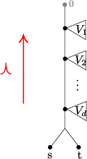
Figure 2. Inductive construction of the partial order $\preceq$, starting from a cherry of the subtree $T_{1}$. Notice that the edge connecting the cherry $\{s,t\}$ to the internal node to which $V_{d}$ is attached could be contracted, as in Figure 3. The grey node labeled with $0$ is the internal node in $T$ to which $T_{1}$ is attached. As before, the edge adjacent to this node could be contracted.

∎

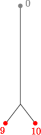
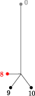
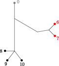
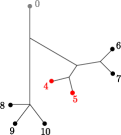
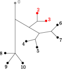
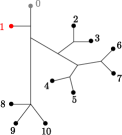
Figure 3. From left to right: inductive definition of the order $\preceq_{a}$ on the leaves of the subtree $T_{a}$ in the right of Figure 1. We add one leaf or one cherry at a time in such a way that the corresponding new leaf or leaves are smaller than the previous ones in the order $\preceq_{a}$. When adding a cherry, we arbitrarily order its two leaves as well (both orderings will be valid). The grey dot with label $0$ in $T_{a}$ corresponds to an internal node of $T$. Broken leaf edges, such as the one in the third tree from the left, should be thought of as straight edges. As in Figure 2, the edge adjacent to the grey node with label $0$ could be contracted.

We now introduce the notion of compatibility of a set with a partial order and a vanishing set. Recall that $J(ij)=J\cap I(ij)$.

Definition 4.8.

Fix two indices $i,j$, a tree $T$ as in the right of Figure 1, and a vanishing set $J$. Let $\preceq$ be a partial order on $[n]\smallsetminus\{i,j\}$ having the cherry property on $T$. Let $I\subset\binom{[n]}{2}$ be a set of size $2(n-2)$ not containing the pair $ij$. We say that $I$ is compatible with $\preceq$ and $J(ij)$ if for each index $a=1,\ldots,m$ and each leaf $k\in T_{a}$, exactly one of the following condition holds:

1. $ik$ and $jk\in I$, and for all $l\prec k$ we have $il$ or $jl\in J(ij)$; or

2. $ik\notin I$, $jl\in I$ for all $l\in T_{a}$, and there exists $t\prec k$ in $T_{a}$ where $it,jt\notin J(ij)$. If $t$ is the maximal element with this property, then $kt\in I$; or

3. $jk\notin I$, $il\in I$ for all $l\in T_{a}$ and there exists $t\prec k$ in $T_{a}$ where $it,jt\notin J(ij)$. If $t$ is the maximal element with this property, then $kt\in I$.

Observe that, for every $k\neq i,j$, at least one of the two elements $ik,jk$ lies in $I$. In addition, the following holds. If $s$ is the maximal element of a subtree $T_{a}$ of size at least two, and $is,js\in I$, we can infer that $il$ or $jl\in J$ for every $l\prec s$, and hence $il,jl\in I$ for every $l\prec s$.

Figure 4 allows us to give a graphical explanation of the compatibility property described above. We fix the tree $T$ with $m=3$ and a partial order $\preceq$ on $[7]$ as in the picture. For each $a=1,2,3$, we let $I_{a}:=\{kl\in I:k\text{ or }l\in T_{a}\}$. Thus, $I=I_{1}\sqcup I_{2}\sqcup I_{3}$. By construction, since $|T_{1}|=1$, we know that $I_{1}=\{i1,j1\}$ independently of the choice of $J$. If $i2$ or $j2$ belong to $J$, then $I_{3}=\{i2,j2,i3,j3\}$ in agreement with condition (i). On the contrary, if $i2,j2\notin J$ then we can choose between $I_{3}=\{i2,j2,j3,32\}$ (since (ii) is satisfied) or $I_{3}=\{i2,j2,i3,32\}$ (so condition (iii) holds). There are many options for $I_{2}$, depending on the set $J_{2}(ij):=\{ik\in J:k\in T_{2}\}\cup\{jk\in J:k\in T_{2}\}$. We provide three examples. If $\emptyset\neq J_{2}(ij)\subseteq\{i4,j4\}$, then we can take either $I_{2}=\{i4,j4,i5,j5,i6,65,i7,76\}$ or $I_{2}=\{i4,j4,i5,j5,j6,65,j7,76\}$. Notice that in both cases $i5,j5\in I_{2}$ by condition (i). If $\emptyset\neq J_{2}(ij)\subseteq\{i7,j7\}$, we can take either $I_{2}=\{i4,j4,i5,54,i6,65,i7,76\}$ or $I_{2}=\{i4,j4,j5,54,j6,65,j7,76\}$. Finally, assume $J_{2}(ij)=\{j5,j6\}$. Then, we may choose $I_{2}=\{i4,j4,i5,54,i6,64,i7,74\}$ or $I_{2}=\{i4,j4,j5,54,j6,64,j7,74\}$.

Figure 4. How to choose the set $I(ij)$ in an example of a tree $T$ with $m=3$. We define the order $\preceq$ as $\{(2,3),(4,5),(4,6),(4,7),(5,6),(5,7),(6,7)\}\cup\{(k,k):1\leqslant k\leqslant 7\}$. By construction, $\preceq$ has the cherry property on $T$ with respect to $i$ and $j$. For any choice of $J$, we have $I_{1}=\{i1,j1\}$. The choices of $I_{2}$ and $I_{3}$ will strongly depend on $J$. We take $I=I_{1}\sqcup I_{2}\sqcup I_{3}$.

Our first result ensures that compatible sets satisfy strong algebraic properties:

Proposition 4.9.

Fix a pair of indices $i,j$, and let $T$ be a tree on $n$ leaves. Let $\preceq$ be a partial order on the set $[n]\smallsetminus\{i,j\}$ that has the cherry property on $T$. Fix a set $J=J(x)$, where $x\in\overline{\mathscr{C}_{T}}\cap\mathcal{T}U_{ij}$, and let $I$ be a set of size $2(n-2)$ that is compatible with $\preceq$ and $J(ij)$. Then:

1. The set of coordinates $\{u_{kl}:kl\in I\}$ is algebraically independent in the function field $\mbox{Quot}(R(ij))$ of the Grassmannian.

2. Let $H=I\cap I(ij)$. Then, the corresponding polynomial subring $K[u_{kl}:kl\in I]$ of $\mbox{Quot}(R(ij))$ fits into a diagram of the form

   (4.5)

   where $\theta(u_{kl})=u_{ik}u_{jl}-u_{il}u_{jk}$ if $kl\notin I(ij)$, and $\theta(u_{kl})=u_{kl}$ otherwise. Furthermore, $\mu$ is the unique map compatible with the inclusions of both rings in $\mbox{Quot}(R(ij))$.

3. For each $l\in[n]\smallsetminus\{i,j\}$, we have

   $$\mu(u_{il}),\mu(u_{jl})\in K[u_{rs}:rs\in I_{\preceq l}][u_{rs}^{-1}:rs\in H_{\preceq l}\smallsetminus J]\text{,}$$

   where $I_{\preceq l}=\{rs\in I:(r\preceq l\mbox{ or }r\in\{i,j\})\mbox{ and }(s\preceq l\mbox{ or }s\in\{i,j\})\}$ and $H_{\preceq l}=H\cap I_{\preceq l}$.

Proof.

Notice that (ii) implies that the elements $\{u_{kl}:kl\in I\}$ in $K[U_{ij}]$ generate the quotient field $\operatorname{\operatorname{Quot}}(R(ij))$ as a transcendental extension of $K$. Thus, it suffices to prove (ii) and (iii).

We first show that the statements hold for $m=1$. We proceed by induction on $n$. If $n=3$, then $T$ is a caterpillar tree and $I=I(ij)$, and there is nothing to prove because $\mu$ is the identity on $R(ij)$. Assume $n>3$ and $I\neq I(ij)$. By symmetry between $i$ and $j$, we suppose that $ik\in I$ and $jk\notin I$ for some $k\neq i,j$. The compatibility of $I$ with $\preceq$ and $J(ij)$ ensures that $\{il:l\neq i,j\}\subset I$.

We let $s$ be the maximal leaf in $T_{1}$ and set $T^{\prime}$ and $T^{\prime}_{1}$ be the trees obtained by removing $s$ from $T$ and $T_{1}$, respectively. Let $\preceq^{\prime}$ be the order on $T^{\prime}$ induced by $\preceq$, and let $J^{\prime}=J\cap\binom{[n]\smallsetminus\{s\}}{2}$ and $I^{\prime}=I\cap\binom{[n]\smallsetminus\{s\}}{2}$. Notice that $J^{\prime}$ is the vanishing set of a point in $\mathcal{T}\!\operatorname{Gr}(2,n-1)$, namely, $J^{\prime}=J(x^{\prime})$, where $x^{\prime}$ is the projection of $x$ to those coordinates not containing the index $s$. The point $x^{\prime}$ belongs to $\overline{\mathscr{C}_{T^{\prime}}}\cap\mathcal{T}U_{ij}^{\prime}$ in $\mathcal{T}\!\operatorname{Gr}(2,n-1)$, where $\mathcal{T}U_{ij}^{\prime}=\{x_{ij}\neq-\infty\}\subset\mathbb{T}\mathbb{P}^{\binom{n-1}{2}-1}$. In addition, $\preceq^{\prime}$ has the cherry property on $T^{\prime}$ with respect to $i$ and $j$.

We define $R(ij)^{\prime}=K[u_{ik},u_{jk}:k\neq i,j,s]$ and $H^{\prime}=I^{\prime}\cap I(ij)$. We know that $I^{\prime}$ is compatible with $\preceq^{\prime}$ and $J^{\prime}(ij)$, so by the inductive hypothesis, it satisfies (ii) and (iii). In particular, we can uniquely define $\mu^{\prime}$ to fit into the diagram

where $\theta^{\prime}$ is the restriction of $\theta$.

We claim that we can extend $\mu^{\prime}$ to a map $\mu$ satisfying (4.5). Since we assumed $I\neq I(ij)$ and $\{il:l\neq i,j\}\subset I$, the observation following Definition 4.8 implies that the element $js$ cannot be in $I$. Instead, there exists $t\neq i,j$ such that $st\in I$, so $I=I^{\prime}\cup\{is,st\}$. We assign $\mu(u_{is}):=u_{is}$ and $\mu(u_{js}):=u_{it}^{-1}(-u_{st}+u_{is}\mu^{\prime}(u_{jt}))$. By the induction hypothesis, we conclude that the image of $\mu$ lies in the algebra $K[u_{kl}:kl\in I][u_{kl}^{-1}:kl\in H\smallsetminus J]$. A straightforward calculation using the Plücker relations shows that $\mu$ and $\theta$ are compatible with the inclusion in the function field $\operatorname{\operatorname{Quot}}R(ij)$. The statement (iii) holds by combining the construction together with the induction hypothesis.

Assume now that $m>1$. For each $a=1,\ldots,m$, we let $I_{a}$ be the subset of $I$ consisting of all pairs involving $i,j$, and the leaves of $T_{a}$. To simplify notation, we identify each tree $T_{a}$ with its set of leaves. Set $I(ij)_{a}=\{ik,jk:k\text{ is a leaf in }T_{a}\}$, $R(ij)_{a}=K[u_{kl}:kl\in I(ij)_{a}]$, and let $H_{a}=I_{a}\cap I(ij)_{a}$. Similarly, we let $\preceq_{a}$ be the restriction of $\preceq$ to the leaves of $T_{a}$ and set $J(ij)_{a}=J\cap I(ij)_{a}$. The order $\preceq_{a}$ has the cherry property on the tree spanned by $\{i,j\}\cup T_{a}$ with respect to $i$ and $j$. Similarly, $J(ij)_{a}$ is the vanishing set of the point $\pi_{a}(x)$, where $\pi_{a}\colon\mathbb{T}\mathbb{P}^{\binom{n}{2}-1}\dashrightarrow\mathbb{T}\mathbb{P}^{\binom{|T_{a}|+2}{2}-1}$ is the projection to those coordinates in $\binom{\{i,j\}\cup T_{a}}{2}$. The point $\pi_{a}(x)$ belongs to the cone $\overline{\mathscr{C}_{\{i,j\}\cup T_{a}}}\cap\pi_{a}(\mathcal{T}U_{ij})$ and $\pi_{a}(\mathcal{T}U_{ij})\subset\{x_{ij}\neq-\infty\}\subset\mathbb{T}\mathbb{P}^{\binom{|T_{a}|+2}{2}-1}$.

By construction, we know that $I=\bigcup_{a=1}^{m}I_{a}$, $\mathord{\preceq}=\bigcup_{a=1}^{m}\mathord{\preceq}_{a}$ and $J(ij)=\bigcup_{a=1}^{m}J(ij)_{a}$. From the $m=1$ case, we know that the set $I_{a}$ satisfies (4.5) for two injective maps $\theta_{a}$ and $\mu_{a}$. We define the maps $\theta$ and $\mu$ associated to the set $I$ by restriction, i.e., $\theta(u_{kl})=\theta_{a}(u_{kl})$ for $kl\in I_{a}$ and $\mu(u_{kl})=\mu_{a}(u_{kl})$ for $kl\in I(ij)_{a}$. Since $\theta_{a}$ and $\mu_{a}$ satisfy (ii) and (iii), the result follows. ∎

Our next result shows that from a partial order $\preceq$ on $[n]\smallsetminus\{i,j\}$ with the cherry property on a tree $T$ and a vanishing set $J$, we can construct a set that is compatible with $\preceq$ and $J(ij)$.

Proposition 4.10.

Assume $T$ is arranged as in the right of Figure 1, and let $\preceq$ be a partial order on $[n]\smallsetminus\{i,j\}$ that has the cherry property on $T$ with respect to $i$ and $j$. Fix a set $J=J(x)$, where $x\in\overline{\mathscr{C}_{T}}\cap\mathcal{T}U_{ij}$. Then, there exists a subset $I=I(ij,T,J)\subset\binom{[n]}{2}$ of size $2(n-2)$ that is compatible with $\preceq$ and $J(ij)$.

Proof.

Let us first consider the case $m=1$. We proceed by induction on $n$. If $n=3$, then $T$ is a caterpillar tree with backbone $\{i,j\}$, and we take $I=I(ij)$. Next, we assume that $n>3$, so $T_{1}$ has more than one leaf. Let $s$ be the maximal leaf in $T_{1}$ with respect to the order $\preceq$. Remove $s$ from $T$ and $T_{1}$, and call $T^{\prime}$ and $T_{1}^{\prime}$ the corresponding subtrees. Let $\preceq^{\prime}$ be the restriction of the order $\preceq$ to the leaves of $T_{1}^{\prime}$. This order has the cherry property on $T^{\prime}$ with respect to $i$ and $j$.

We let $J^{\prime}=J\cap\binom{[n]\smallsetminus\{s\}}{2}$. As in the proof of Proposition 4.9, $J^{\prime}$ is the vanishing set of the point $x^{\prime}$, obtained by removing from $x$ all those coordinates involving the index $s$. The point $x^{\prime}$ lies in $\overline{\mathscr{C}_{T^{\prime}}}\cap\mathcal{T}U_{ij}^{\prime}\subset\mathcal{T}\!\operatorname{Gr}(2,n-1)$. By the inductive hypothesis, there is a subset $I^{\prime}=I(ij,T^{\prime},J^{\prime})$ of $\binom{[n]\smallsetminus\{s\}}{2}$ of size $2(n-3)$ that is compatible with $\preceq^{\prime}$ and $J^{\prime}(ij)$. Furthermore, the set $H^{\prime}=I^{\prime}\cap I(ij)$ satisfies $H^{\prime}\supset\{il:l\in T_{1}^{\prime}\}$ or $H^{\prime}\supset\{jl:l\in T_{1}^{\prime}\}$.

We define $I=I(ij,T,J)$ by adding two elements to $I^{\prime}$. We have a priori two possible scenarios. First, assume that, for all $l\neq i,j,s$, we have $il$ or $jl$ belonging to $J$. In this case, we define $I=I^{\prime}\cup\{is,js\}=I(ij)$. In other case, there exists $l\neq i,j,s$ with $il,jl\notin J$. We let $t$ be the maximal leaf with that property with respect to the partial order $\preceq^{\prime}$. In this case, we have two valid options to define $I$, namely,

$$I:=I^{\prime}\cup\{st,is\}\text{ or }I:=I^{\prime}\cup\{st,js\}.$$

To decide which one to choose, we proceed as follows. If $H^{\prime}\supset\{il:l\in T_{1}^{\prime}\}$, then we take $I=I^{\prime}\cup\{st,is\}$. If $H^{\prime}\supset\{jl:l\in T_{1}^{\prime}\}$, then we take $I=I^{\prime}\cup\{st,js\}$. If $H^{\prime}$ contains both sets $\{il:l\in T_{1}^{\prime}\}$ and $\{jl:l\in T_{1}^{\prime}\}$, both options are valid and we must choose one of them. Note that $H=I\cap I(ij)$ satisfies $H\supset\{il:l\neq i,j\}$ or $H\supset\{jl:l\neq i,j\}$. By construction, $I$ is compatible with $\preceq$ and $J(ij)$.

We now prove the statement for general $m$. We keep the notation from the proof of Proposition 4.9. For each $a=1,\ldots,m$, we let $\preceq_{a}$ be the restriction of $\preceq$ to the leaf set of each $T_{a}$, and similarly we define $J_{a}$ as the subset of $J$ consisting of pairs in $\{i,j\}\cup T_{a}$. The order $\preceq_{a}$ has the cherry property on the tree spanned by the leaves of $T_{a}$, $i$, and $j$, with respect to the indices $i$ and $j$. Similarly, $J_{a}$ is the vanishing set of the projection $\pi_{a}(x)$ to the coordinates indexed by pairs in $\{i,j\}\cup T_{a}$. The point $\pi_{a}(x)$ belongs to $\overline{\mathscr{C}_{\{i,j\}\cup T_{a}}}\cap\pi_{a}(\mathcal{T}U_{ij})$. From the $m=1$ case, we construct sets $I_{a}=I_{a}(ij,T_{a},J_{a})$ that are compatible with $\preceq_{a}$ and $J_{a}(ij)$ for each $a$. We define

$$I=I(ij,T,J)=\bigcup_{a=1}^{m}I_{a}(ij,T_{a},J_{a}).$$

By construction, $I$ is compatible with $\preceq$ and $J(ij)$. This concludes our proof. ∎

Remark 4.11.

From the proof of Proposition 4.10, we see that the set $I$ is not uniquely determined by $\preceq$, $J$ and $i,j$. This is so because for every $a=1,\ldots,m$, one of the following is true: either $H\supset\{il:l\in T_{a}\}$ or $H\supset\{jl:l\in T_{a}\}$, and we can choose freely between any of these two options. In particular, there is one choice of the set $I$ for which $H\supset\{il:l\neq i,j\}$ and one choice for which $H\supset\{jl:l\neq i,j\}$. Allowing the flexibility to choose among two options for each $H_{a}=I_{a}\cap I(ij)$ whenever possible preserves the symmetry of our objects with respect to $i$ and $j$, and will simplify our proofs.

Observe that $H\supset\{il,jl:l\in T_{a}\}$ if and only if either $T_{a}$ has exactly one leaf, or, for every $k\in T_{a}$ that is not maximal with respect to $\preceq$, we have $il\in J_{a}$ or $jl\in J_{a}$. The reason for imposing this condition comes from the Plücker relations.

Notice that the properties of Proposition 4.9 ensure that $\mu(u_{kl})=u_{kl}$ for all $kl\in H$. We use this observation in the following two examples and in the remainder of this Section.

Example 4.12.

Let $T$ be a caterpillar tree with backbone spanned by $i$ and $j$. When setting $\preceq$ as $\{(k,k):k\neq i,j\}$, $I=I(ij)$, $\theta=\operatorname{id}$ and $\mu=\operatorname{\operatorname{inc}}$, we recover the results from Section 4.1. $\diamond$

Example 4.13.

Let $i=1,j=2$ and $T$ be a trivalent tree on four leaves with cherry $\{1,2\}$. Then, we take $\preceq$ to be $\{(3,3),(3,4),(4,4)\}$. If $13,23\notin J(12)$, we let $I=\{13,23,34,14\}$, and $\mu$ be the map defined by $\mu(u_{24})=u_{13}^{-1}(u_{34}+u_{14}u_{23})$ and $\mu(u_{kl})=u_{kl}$ if $kl=13,23$ or $14$.

On the contrary, if $J(12)$ contains either $13$ or $23$, we define $I=\{13,23,14,24\}=I(12)$ and let $\mu$ be the inclusion map. $\diamond$

In what follows, we outline the construction of a section to $\operatorname{trop}$ over a covering of $\mathcal{T}U_{ij}$. Given a tree $T$ on $n$ leaves and a vanishing set $J=J(x)$ associated to a point $x\in\overline{\mathscr{C}_{T}}\cap\mathcal{T}U_{ij}$, we choose a partial order with the cherry property on $T$ as in Lemma 4.7 and a compatible set $I=I(ij,T,J)$ as in Proposition  4.10. We define the map

(4.6) $$\sigma_{T,I,J}^{(ij)}\colon\mathscr{C}^{(ij)}_{T,J}\lhook\joinrel\longrightarrow\mathcal{T}U_{ij}\longrightarrow(\operatorname{\operatorname{Spec}}K[u_{kl}:kl\in I])^{\operatorname{an}}\quad\text{ by }\quad\sigma_{T,I,J}^{(ij)}(x)={\sigma}^{(ij)}_{I}(x)\text{.}$$

The next result show that all points in the image of $\sigma^{(ij)}_{T,I,J}$ are multiplicative seminorms on the localization $K[u_{kl}:kl\in I]_{S_{H\smallsetminus J}}$:

Lemma 4.14.

Let $i,j$, $T$, $\preceq$, and $J$ be as above. Assume that $I$ is compatible with $\preceq$ and $J(ij)$. Then, given any point $x\in\mathscr{C}^{(ij)}_{T,J}$, the seminorm $\sigma^{(ij)}_{T,I,J}(x)$ as defined in (4.6) extends uniquely to a multiplicative seminorm on $K[u_{kl}:kl\in I][u_{kl}^{-1}:kl\in H\smallsetminus J]$, that is, to an element of $(\operatorname{\operatorname{Spec}}K[u_{kl}:kl\in I][u_{kl}^{-1}:kl\in H\smallsetminus J])^{\operatorname{an}}\subset U_{ij}^{\operatorname{an}}$.

Proof.

Since $\sigma^{(ij)}_{T,I,J}(x)(u_{kl})=\exp(x_{kl}-x_{ij})\neq 0$ for all $kl\in H\smallsetminus J$, we can uniquely extend this multiplicative seminorm to the Laurent polynomial ring $K[u_{kl}:kl\in I][u_{kl}^{-1}:kl\in H\smallsetminus J]$. ∎

The following lemma guarantees that the ideal $\mathfrak{a}_{J(ij)}$ maps to $0$ under $\sigma^{(ij)}_{T,I,J}(x)$.

Lemma 4.15.

Let $i,j$, $T$, $\preceq$, and $J$ be as above. Then, $\sigma^{(ij)}_{T,I,J}(x)(\mathfrak{a}_{J(ij)})=0$ for all $x\in\mathscr{C}^{(ij)}_{T,J}$.

Proof.

For simplicity, we write $\sigma(x)=\sigma^{(ij)}_{T,I,J}(x)$. By symmetry between $i$ and $j$, it suffices to show that $\sigma(x)(u_{jl})=0$ for all $jl\in J(ij)$. If $jl\in J(ij)\cap I$, then $\sigma(x)(u_{jl})=\exp(x_{jl}-x_{ij})=0$.

On the contrary, assume $jl\in J(ij)\smallsetminus I$. Since $I$ is compatible with $\preceq$ and $J(ij)$, and $jl\notin I$, this implies that $il\in I$, and there exists $t\prec l$ maximal such that $it,jt\notin J$, forcing $lt,it\in I$ and $\mu(u_{jl})=u_{it}^{-1}(-u_{lt}+u_{il}\,\mu(u_{jt}))$. Lemma 4.4 ensures that $il\in J(ij)$, so $\sigma(x)(u_{il})=0$. The four-point condition on the quartet $\{i,j,t,l\}$ implies that $x_{lt}+x_{ij}=-\infty$, so $x_{lt}=-\infty$ and thus $\sigma(x)(u_{lt})=0$. The definition of $\mu(u_{jl})$, together with the non-Archimedean triangle inequality for $\sigma(x)$, yield

$$\sigma(x)(u_{jl})=\sigma(x)(u_{it}^{-1})\sigma(x)(-u_{lt}+u_{il}\,\mu(u_{jt}))\leqslant\sigma(x)(u_{it}^{-1})\max\{\sigma(x)(u_{lt}),\sigma(x)(u_{il})\sigma(x)(u_{jt})\}=0.\qed$$

By Proposition 4.9 (ii), the map $\mu$ induces an isomorphism of localizations

where $S_{H\smallsetminus J}$ is as in Remark 4.1. Using this map and Lemma 4.14, we define $\sigma^{(ij)}_{T,I,J}(x)$ on $R(ij)$ by restriction.

We now state the main result in this Section, keeping the previous notation.

Theorem 4.16.

Let $i,j$, $T$, $\preceq$, and $J$ be as above, and let $I=I(ij,T,J)$ be a set of size $2(n-2)$ that is compatible with $\preceq$ and $J(ij)$. Then, $\sigma^{(ij)}_{T,I,J}$ is a section to the tropicalization map over the cone $\mathscr{C}^{(ij)}_{T,J}$.

Proof.

We divide the proof in two parts. First, we discuss the case when $m=1$, and second, we show how the general result can be deduced from this special case. Using the diagram (4.5) and the Plücker relations, we view all functions $u_{kl}:=u_{ik}u_{jl}-u_{il}u_{jk}$ in the ring $R(ij)$. By Lemma 4.14, we can define $\sigma^{(ij)}_{T,I,J}(x)$ on this ring. For simplicity, write $\sigma:=\sigma^{(ij)}_{T,I,J}$.

In what follows, we consider polynomials in all variables $\{u_{kl}:kl\neq ij\}$. To simplify notation, rather than writing $\mu(u_{kl})$, we underline the variable $u_{kl}$ whenever $kl\in I(ij)\smallsetminus I$, indicating that we should consider its image under $\mu$ in $K[u_{kl}:kl\in I][u_{kl}^{-1}:kl\in H\smallsetminus J]$.

Assume $m=1$. We proceed by induction on $n$ and use Lemma 4.2 to check the section property. If $n=3$, then $T$ is the caterpillar tree, and so $I=I(ij)$. The result follows by Proposition 4.5. Next, suppose that $n>3$, and let $s$ be the maximal element in $T_{1}$. Let $T^{\prime}$ and $T_{1}^{\prime}$ be the trees obtained by removing the leaf $s$ from $T$ and $T_{1}$, respectively. We keep the notation from the proof of Proposition 4.9 and define $I^{\prime}=I\cap\binom{[n]\smallsetminus\{s\}}{2}$, $J^{\prime}=J\cap\binom{[n]\smallsetminus\{s\}}{2}$, $R(ij)^{\prime}=K[u_{ik},u_{jk}:k\neq i,j,s]$. We also let $\preceq^{\prime}$ be the order on $T^{\prime}_{1}$ induced by $\preceq$. Since $I^{\prime}$ is compatible with $\preceq^{\prime}$ and $J^{\prime}(ij)$, we find that the restriction of $\sigma(x)$ to $R(ij)^{\prime}$ agrees with $\sigma^{(ij)}_{T^{\prime},I^{\prime},J^{\prime}}(x^{\prime})$, where $x^{\prime}$ is the projection of $x$ to those coordinates not involving the index $s$. It suffices to prove that $\sigma(x)(u_{sl})=\exp(x_{sl}-x_{ij})$ for all $l\neq s$. All other identities will follow by the inductive hypothesis. Using the symmetry between $i$ and $j$, we suppose that $\{il:l\neq i,j\}\subset H$ (see Remark 4.11). We analyze two cases, depending on the nature of $I$.

Case 1: Assume that for all $l\neq i,j,s$ we have $il$ or $jl\in J$. In this situation, we have $I=I(ij)$. In particular, $\sigma(x)(u_{is})=\exp(x_{is}-x_{ij})$ and $\sigma(x)(u_{js})=\exp(x_{js}-x_{ij})$.

Fix an index $l\neq i,j,s$. By the four-point condition on the quartet $\{i,j,s,l\}$, we have $x_{sl}+x_{ij}=x_{il}+x_{js}=x_{jl}+x_{is}=-\infty$, so $u_{sl}=u_{is}u_{jl}-u_{il}u_{js}\in\mathfrak{a}_{J(ij)}$. Lemma 4.15 implies $\sigma(x)(u_{sl})=0=\exp(x_{sl}-x_{ij})$, as we wanted to show.

Case 2: Suppose that there exists $t\neq i,j,s$ satisfying $it,jt\notin J$. Choose $t$ maximal with this property. By Definition 4.8, we know that $st\in I$, so $\sigma(x)(u_{st})=\exp(x_{st}-x_{ij})$. Similarly, since $is\in I$ we have $\sigma(x)(u_{is})=\exp(x_{is}-x_{ij})$. Using the identity

$$\underline{u_{js}}=u_{it}^{-1}u_{is}\,\underline{u_{jt}}-u_{it}^{-1}u_{st},$$

we compute $\sigma(x)(u_{js})$ by expanding $\underline{u_{jt}}$ as a polynomial in the $I$-coordinates, and taking the maximum over the values on all monomials occurring in $\underline{u_{js}}$. By Proposition 4.9 (iii), the monomial $u_{it}^{-1}u_{st}$ does not cancel with any term in $u_{it}^{-1}u_{is}\,\underline{u_{jt}}$. Since $\sigma(x)$ is multiplicative and it satisfies $\sigma(x)(u_{kl})=\exp(x_{kl}-x_{ij})$ for all $kl\in I$ as well as $\sigma(x)(u_{jt})=\exp(x_{jt}-x_{ij})$ by the inductive hypothesis, we deduce

$$\sigma(x)(u_{js}) =\sigma(x)(u_{it}^{-1}u_{is}\,\underline{u_{jt}}-u_{it}^{-1}u_{st})=\max\{\sigma(x)(u_{it}^{-1}u_{is}\,\underline{u_{jt}}),\sigma(x)(u_{it}^{-1}u_{st})\}$$

$$=\max\{\exp(-x_{it}+x_{is})\sigma(x)(\underline{u_{jt}}),\,\exp(-x_{it}+x_{st})\}$$

$$=\max\{\exp(-x_{it}+x_{is}+x_{jt}-x_{ij}),\,\exp(-x_{it}+x_{st})\}.$$

The four-point condition on the quartet $\{i,j,s,t\}$ yields $\sigma(x)(u_{js})=\exp(x_{js}-x_{ij})$.

Finally, we prove the claim for $u_{sl}$, where $l\neq i,j,s,t$. First, assume that $t\prec l$. Then, the maximality of $t$ and Lemma 4.4 imply that both $il$ and $jl$ belong to $J$, hence $u_{sl}\in\mathfrak{a}_{J(ij)}$ and $\sigma(x)(u_{sl})=0$ by Lemma 4.15. The four-point condition on $\{i,j,s,l\}$ yields $x_{sl}=-\infty$, and the result holds.

On the contrary, suppose that $l\prec t$. By the Plücker relations, we write $u_{sl}$ as

$$u_{sl}=u_{it}^{-1}u_{is}{u_{tl}}+u_{it}^{-1}u_{il}u_{st}.$$

In order to evaluate $\sigma(x)$ on $u_{sl}$, we expand $u_{tl}$ in $I$-coordinates and then take the maximum over the values of $\sigma(x)$ on all monomials. By Proposition  4.9 (iii), the monomial $u_{it}^{-1}u_{il}u_{st}$ does not cancel with any term in the expansion of $u_{it}^{-1}u_{is}{u_{tl}}$. Note that $\sigma(x)(u_{tl})=\exp(x_{tl}-x_{ij})$ by the inductive hypothesis. Since $\sigma(x)$ is multiplicative and it satisfies $\sigma(x)(u_{pq})=\exp(x_{pq}-x_{ij})$ for all $pq\in I$, this implies

$$\sigma(x)(u_{sl}) =\max\{\sigma(x)(u_{it}^{-1}u_{is}\,{u_{tl}}),\sigma(x)(u_{it}^{-1}u_{il}u_{st})\}$$

$$=\max\{\exp(-x_{it}+x_{is})\sigma(x)({u_{tl}}),\,\exp(-x_{it}+x_{il}+x_{st}-x_{ij})\}$$

$$=\max\{\exp(-x_{it}+x_{is}+x_{tl}-x_{ij}\},\,\exp(-x_{it}+x_{il}+x_{st}-x_{ij})\}.$$

Since $l\prec t\prec s$, and $\preceq$ has the cherry property on $T$ with respect to $i$ and $j$, we know by Definition 4.6 (iii) that either $\{l,t\}$ or $\{t,s\}$ are cherries of the quartet $\{i,l,t,s\}$. Therefore, one of the following identities hold:

$$x_{is}+x_{tl}\leqslant x_{it}+x_{sl}=x_{il}+x_{st}\quad\text{ or }\quad x_{il}+x_{st}\leqslant x_{it}+x_{sl}=x_{is}+x_{tl}.$$

In both cases it is easy to check that $\sigma(x)(u_{sl})=\exp(x_{sl}-x_{ij})$.

Next, we discuss the case when $m>1$. As before, we show that $\sigma(x)(u_{kl})=\exp(x_{kl}-x_{ij})$ for all $kl\in\binom{[n]}{2}\smallsetminus\{ij\}$. We follow the notation of Figure 1. Proposition 4.9 (iii) and the proof for the $m=1$ case guarantee that the result holds when $kl\in I(ij)$ or when we pick two indices $k,l$ in the same subtree $T_{a}$, for $a=1,\ldots,m$.

It remains to check the case when $k$ and $l$ belong to two different subtrees, say $k\in T_{a}$ and $l\in T_{b}$ with $a\neq b$. The quartet with leaves $\{i,j,k,l\}$ contains the cherry $\{i,k\}$ or the cherry $\{i,l\}$. Hence, by the four-point condition, one of the following is true:

(4.7) $$x_{ik}+x_{jl}\leqslant x_{ij}+x_{kl}=x_{il}+x_{jk}\quad\mbox{ or }\quad x_{il}+x_{jk}\leqslant x_{ij}+x_{kl}=x_{ik}+x_{jl}.$$

We distinguish four cases. If $ik,jk\in H$, then $u_{kl}=u_{ik}\,\underline{u_{jl}}-\underline{u_{il}}u_{jk}$. The compatibility of $I$ with $\preceq$ and $J(ij)$, and Proposition 4.9 (iii) ensure that none of the monomials in $u_{ik}\,\underline{u_{jl}}$ cancel out with any monomial in $\underline{u_{il}}u_{jk}$. Using (4.7) we conclude that

$$\sigma(x)(u_{kl})=\max\{\exp(x_{ik}+x_{jl}-2x_{ij}),\,\exp(x_{il}+x_{jk}-2x_{ij})\}=\exp(x_{kl}-x_{ij}).$$

An analogous argument holds when $il,jl\in H$.

It remains to study the situation where both pairs $ik,jk$ and $il,jl$ have one member outside $H$. In particular, by Definition 4.8, we know that $T_{a}$ and $T_{b}$ have more than one leaf. By the symmetry between $i$ and $j$, we are left with two possibilities: either $ik,jl\notin H$ or $ik,il\notin H$. By the compatibility of $I$ with $\preceq$ and $J(ij)$, we know that there exist maximal elements $k^{\prime}\prec k$ and $l^{\prime}\prec l$, satisfying that $kk^{\prime},ll^{\prime}\in I$, and $ik^{\prime},jk^{\prime},il^{\prime},jl^{\prime}\notin J$.

Let us discuss the first scenario, where $ik,jl\notin H$. Notice that $H\supset\{jq:q\in T_{a}\}\cup\{iq:q\in T_{b}\}$ by Remark 4.11. We write $u_{kl}=\underline{u_{ik}}\underline{u_{jl}}-u_{il}u_{jk}$. Proposition 4.9 (iii) shows that the expansion of $\underline{u_{ik}}\underline{u_{jl}}$ in $I$-coordinates does not contain the monomial $u_{il}u_{jk}$. Hence, by (4.7) we conclude

$$\sigma(x)(u_{kl}) =\max\{\sigma(x)(\underline{u_{ik}}\underline{u_{jl}}),\sigma(x)(u_{il}u_{jk})\}$$

$$=\max\{\exp(x_{ik}+x_{jl}-2x_{ij}),\exp(x_{il}+x_{jk}-2x_{ij})\}=\exp(x_{kl}-x_{ij}).$$

Finally, let us analyze the case when $ik,il\notin H$. In this situation, we know that $H\supset\{jq:q\in T_{a}\cup T_{b}\}$, and we have $u_{kl}=\underline{u_{ik}}u_{jl}-\underline{u_{il}}u_{jk}$, where

$$\underline{u_{ik}}=u_{jk^{\prime}}^{-1}(-u_{kk^{\prime}}+\underline{u_{ik^{\prime}}}u_{jk})\qquad\text{and}\qquad\underline{u_{il}}=u_{jl^{\prime}}^{-1}(-u_{ll^{\prime}}+\underline{u_{il^{\prime}}}u_{jl}).$$

Plugging these expressions into the Plücker expression for $u_{kl}$, we see that

$$u_{kl}=\underline{u_{ik}}u_{jl}-\underline{u_{il}}u_{jk}=u_{jk}u_{jl}(u_{jk^{\prime}}^{-1}\,\underline{u_{ik^{\prime}}}-u_{jl^{\prime}}^{-1}\,\underline{u_{il^{\prime}}})-u_{jk^{\prime}}^{-1}u_{kk^{\prime}}u_{jl}+u_{jl^{\prime}}^{-1}u_{ll^{\prime}}u_{jk}.$$

The conditions that $k^{\prime}\prec k$ and $l^{\prime}\prec l$ together with Proposition 4.9 (iii) ensure that the monomials $u_{jl}u_{kk^{\prime}}u_{jk^{\prime}}^{-1}$ and $u_{jl^{\prime}}^{-1}u_{ll^{\prime}}u_{jk}$ cannot be present in the polynomial $u_{jk}u_{jl}(u_{jk^{\prime}}^{-1}\,\underline{u_{ik^{\prime}}}-u_{jl^{\prime}}^{-1}\,\underline{u_{il^{\prime}}})$. Hence,

$$\sigma(x)(u_{kl})=\max\{\sigma(x)(u_{jk}u_{jl}(u_{jk^{\prime}}^{-1}\,\underline{u_{ik^{\prime}}}-u_{jl^{\prime}}^{-1}\,\underline{u_{il^{\prime}}}),\sigma(x)(u_{jl}u_{kk^{\prime}}u_{jk^{\prime}}^{-1}),\sigma(x)(u_{jl^{\prime}}^{-1}u_{ll^{\prime}}u_{jk})\}.$$

We now study these three terms, starting from the last two. Since $k,k^{\prime}\in T_{a}$ and $l,l^{\prime}\in T_{b}$, we deduce from the four-point conditions on the quartets $\{j,l,k,k^{\prime}\}$ and $\{j,k,l,l^{\prime}\}$ that

$$\sigma(x)(u_{jl}u_{kk^{\prime}}u_{jk^{\prime}}^{-1})\leqslant\exp(x_{kl}-x_{ij})\quad\text{and}\quad\sigma(x)(u_{jl^{\prime}}^{-1}u_{ll^{\prime}}u_{jk})\leqslant\exp(x_{kl}-x_{ij}).$$

We claim that the value of $\sigma(x)$ at the polynomial $u_{jk}u_{jl}(u_{jk^{\prime}}^{-1}\,\underline{u_{ik^{\prime}}}-u_{jl^{\prime}}^{-1}\,\underline{u_{il^{\prime}}})$ equals $\exp(x_{kl}-x_{ij})$. As before, by Proposition 4.9 (iii), we know that both expressions $u_{jk^{\prime}}^{-1}\,\underline{u_{ik^{\prime}}}$ and $u_{jl^{\prime}}^{-1}\,\underline{u_{il^{\prime}}}$ involve disjoint sets of monomials, so no cancellations can occur. The four-point conditions on the quartets $\{i,j,k^{\prime},k\}$, $\{i,j,l^{\prime},l\}$ imply $x_{jk}+x_{ik^{\prime}}=x_{ik}+x_{jk^{\prime}}$ and $x_{jl}+x_{il^{\prime}}=x_{il}+x_{jl^{\prime}}$, so

$$\sigma(x)(u_{jk}u_{jl}u_{jk^{\prime}}^{-1}\,\underline{u_{ik^{\prime}}}) =\exp(x_{jk}+x_{jl}-x_{jk^{\prime}}+x_{ik^{\prime}}-2x_{ij})=\exp(x_{ik}+x_{jl}-2x_{ij}),$$

$$\sigma(x)(u_{jk}u_{jl}u_{jl^{\prime}}^{-1}\,\underline{u_{il^{\prime}}}) =\exp(x_{jk}+x_{jl}-x_{jl^{\prime}}+x_{il^{\prime}}-2x_{ij})=\exp(x_{jk}+x_{il}-2x_{ij}).$$

Hence, $\sigma(x)(u_{kl})=\max\{\exp(x_{ik}+x_{jl}-2x_{ij}),\exp(x_{jk}+x_{il}-2x_{ij})\}=\exp(x_{kl}-x_{ij})$ by  (4.7). This concludes our proof. ∎

4.3. Uniqueness and continuity

In the previous two Sections, we constructed explicit maps $\sigma^{(ij)}_{T,I,J}$ on a covering of $\mathcal{T}\!\operatorname{Gr}(2,n)$ by cones labeled $\mathscr{C}^{(ij)}_{T,J}$, and we showed that these maps are a section to $\operatorname{trop}$ on each domain. Our next task is to glue these sections together and, thus, define a map over $\mathcal{T}\!\operatorname{Gr}(2,n)$. In order to do so, we show that these sections are the unique ones satisfying a maximality property. In Section 5 we give a more conceptual proof of this fact via the existence of a unique Shilov boundary point in the fibers of the tropicalization map.

Lemma 4.17.

Let $x\in\mathcal{T}\!\operatorname{Gr}(2,n)$ and $i,j$ be such that $x\in\mathcal{T}U_{ij}$. Let $T$ and $J$ be such that $x\in\mathscr{C}^{(ij)}_{T,J}$. Then, for any index set $I$ compatible with $\preceq$ and $J(ij)$, and for any $\rho\in\operatorname{trop}^{-1}(x)$, we have that

$$\rho(f)\leqslant\sigma^{(ij)}_{T,I,J}(x)(f)\qquad\text{ for all }f\in R(ij).$$

Proof.

Let $H=I\cap I(i,j)$ be as in Sections 4.1 and 4.2. Since $\rho$ and $\sigma^{(ij)}_{T,I,J}(x)$ belong to the fiber of $\operatorname{trop}$ over $x$, Lemma 4.2 ensures that $\rho(u_{kl})=\exp(x_{kl}-x_{ij})=\sigma^{(ij)}_{T,I,J}(x)(u_{kl})$ for all $k,l$.

Notice that since $\rho(u_{kl})\neq 0$ for any $kl\in H\smallsetminus J$, we can uniquely extend the seminorm $\rho$ from $R(ij)$ to the Laurent polynomial ring $K[u_{kl}:kl\in I][u_{kl}^{-1}:kl\in H\smallsetminus J]$ via the map $\mu$ in (4.5), as we did in Lemma 4.14. For simplicity, we also call this extension by $\rho$. Given any polynomial $f\in R(ij)$, we write it as a Laurent polynomial $f=\sum_{\alpha}c_{\alpha}u^{\alpha}$, where $\alpha\in\mathbb{N}_{0}^{I\smallsetminus(H\smallsetminus J)}\times\mathbb{Z}^{H\smallsetminus J}$. The definition of the map $\sigma^{(ij)}_{T,I,J}$ and the non-Archimedean triangle inequality for $\rho$ ensure that

$$\rho(f)\leqslant\max\limits_{\alpha}\{\rho(c_{\alpha}u^{\alpha})\}=\max_{\alpha}\{|c_{\alpha}|\sigma^{(ij)}_{T,I,J}(x)(u^{\alpha})\}=\sigma^{(ij)}_{T,I,J}(x)(f)\text{.}\qed$$

The intrinsic characterization of the maps $\sigma^{(ij)}_{T,I,J}$ in Lemma 4.17 has two important consequences. First, the function $\sigma^{(ij)}_{T,I,J}$ is independent of the choice of the index set $I$ as long as it is compatible with $\preceq$ and $J(ij)$. Likewise, the functions $\sigma^{(ij)}_{T,I,J}$ and $\sigma^{(ij)}_{T^{\prime},I^{\prime},J^{\prime}}$ agree on the overlaps of the sets $\mathscr{C}^{(ij)}_{T,J}$ and $\mathscr{C}^{(ij)}_{T^{\prime},J^{\prime}}$, corresponding to two trees and two vanishing sets. Therefore, these functions glue together to yield a unique map $\sigma^{(ij)}$ on $\mathcal{T}U_{ij}$ for every choice of a pair $ij$.

Our next result ensures that the collection $\{\sigma^{(ij)}\}_{ij}$ glues to a map $\sigma\colon\mathcal{T}\!\operatorname{Gr}(2,n)\to\operatorname{Gr}(2,n)^{\operatorname{an}}$.

Proposition 4.18.

The map $\sigma^{(ij)}$ is independent of our starting choice of indices $i$ and $j$.

Proof.

The result follows from Lemma 4.17, as we now explain. Fix two pairs of indices $ij,pq\in\binom{[n]}{2}$, and pick any point $x\in\mathcal{T}U_{ij}\cap\mathcal{T}U_{pq}$, so $x_{ij},x_{pq}\neq-\infty$. Let $J=J(x)$ and fix a tree $T$ with $x\in\overline{\mathscr{C}_{T}}$. The multiplicative seminorm $\sigma^{(ij)}(x)$ is defined over $R(ij)$, whereas $\sigma^{(pq)}(x)$ is defined over $R(pq)$. To avoid confusions, we denote by $u_{kl}$ the functions in $R(ij)$ and by $v_{kl}$ the functions in $R(pq)$. As usual, we write $u_{kl}=u_{ik}u_{jl}-u_{ik}u_{jl}$ in $R(ij)$ whenever $kl\notin I(ij)$, and $v_{kl}=v_{pk}v_{ql}-v_{pl}v_{qk}$ in $R(pq)$ whenever $kl\notin I(pq)$.

Since $x\in\mathcal{T}U_{ij}\cap\mathcal{T}U_{pq}$, we know that $\sigma^{(ij)}(x)(u_{pq})=\exp(x_{pq}-x_{ij})\neq 0$ and $\sigma^{(pq)}(x)(v_{ij})=\exp(x_{ij}-x_{pq})\neq 0$. Thus, the multiplicative seminorms $\sigma^{(ij)}(x)$ and $\sigma^{(pq)}(x)$ extend uniquely to the localizations $R(ij)_{S_{\{pq\}}}$ and $R(pq)_{S_{\{ij\}}}$ defined as in Remark 4.1. These localizations are related by the natural isomorphism

$$r\colon R(pq)_{S_{\{ij\}}}\longrightarrow R(ij)_{S_{\{pq\}}},\qquad v_{pk}\longmapsto u_{pk}/u_{pq}\quad\text{ and }\quad v_{qk}\longmapsto u_{qk}/u_{pq}\text{.}$$

Both seminorms $\sigma^{(ij)}(x)$ and $\sigma^{(pq)}(x)$ are maximal with respect to evaluation on these localizations. By Lemma 4.17, $\sigma^{(ij)}(x)\circ r=$ $\sigma^{(pq)}(x)$ on $R(pq)_{S_{\{ij\}}}$, as we wanted to show. ∎

Theorem 4.16 shows that $\sigma$ is a section to $\operatorname{trop}$. We end by proving the continuity of $\sigma$.

Theorem 4.19.

The map $\sigma\colon\mathcal{T}\!\operatorname{Gr}(2,n)\to\operatorname{Gr}(2,n)^{\operatorname{an}}$ is continuous.

Proof.

Since the sets $U_{ij}$ for $ij\in\binom{[n]}{2}$ are an open cover of $\operatorname{Gr}(2,n)$, it suffices to prove that each restriction $\sigma^{(ij)}\colon\mathcal{T}U_{ij}\to U_{ij}^{\operatorname{an}}$ is continuous. Recall that the topology on $U_{ij}^{\operatorname{an}}$ is the topology of pointwise convergence on functions in the coordinate ring $R(ij)$. Given a sequence $(x^{(m)})_{m\in\mathbb{N}}\subset\mathcal{T}U_{ij}$ converging to $x\in\mathcal{T}U_{ij}$ and any element $f\in R(ij)$, we wish to show that the sequence $\sigma(x^{(m)})(f)$ has a limit and, moreover, that its limit is $\sigma(x)(f)$. Equivalently,

(4.8) $$\sigma(x)(f)\leqslant\liminf_{m}\,\sigma(x^{(m)})(f)\leqslant\limsup_{m}\,\sigma(x^{(m)})(f)\leqslant\sigma(x)(f)\qquad\text{ for all }f\in R(ij).$$

It suffices to prove that any subsequence of $(x^{(m)})_{m}$ has a sub-subsequence satisfying (4.8).

In order to establish the desired inequalities, we set some notation. From the topology of $\mathcal{T}\!\operatorname{Gr}(2,n)$, we know that $\lim\limits_{m\to\infty}x^{(m)}_{kl}-x^{(m)}_{ij}=x_{kl}-x_{ij}$ in $\overline{\mathbb{R}}$ for all $kl\in\binom{[n]}{2}$. In addition, by the pigeonhole principle, any subsequence of $(x^{(m)})_{m}$ has a subsequence $(x^{(m_{k})})_{k}$ satisfying $J(x^{(m_{k})})=J(x^{(m_{l})})=:\tilde{J}\subset J$ for all $k,l\in\mathbb{N}$, as well as $(x^{(m_{k})})_{k}\subset\mathscr{C}^{(ij)}_{T,\tilde{J}}$ and $x\in\mathscr{C}^{(ij)}_{T,J}$ for the same tree $T$. To simplify notation, we assume the original sequence has this property. The result follows from Lemmas  4.20 and 4.21 below.∎

Lemma 4.20.

Fix a pair of indices $i,j$ in $[n]$, an arbitrary tree type $T$ on $n$ leaves and a point $x\in\mathscr{C}^{(ij)}_{T,J}$. Suppose that there is a vanishing set $\tilde{J}\subset J$ and a sequence $(x^{(m)})_{m}$ in the cone $\mathscr{C}^{(ij)}_{T,\tilde{J}}$ converging to $x$. Then,

$$\limsup\limits_{m}\,\sigma^{(ij)}(x^{(m)})(f)\leqslant\sigma^{(ij)}(x)(f)\qquad\text{ for all }f\in R(ij).$$

Proof.

We let $\tilde{I}=I(ij,T,\tilde{J})$ and $I=I(ij,T,J)$ be two compatible sets, and set $\tilde{H}=\tilde{I}\cap I(ij)$, $H=I\cap I(ij)$. We construct $\sigma(x^{(m)})$ and $\sigma(x)$ using formula (4.6). Since $\sigma$ is independent of all choices of index sets, we may assume that both $I$ and $\tilde{I}$ are compatible with the same order $\preceq$ on $[n]\smallsetminus\{i,j\}$ having the cherry property on $T$, and that $\tilde{H}$ satisfies $\tilde{H}\subset H$ by Remark 4.11. Since $\tilde{J}\subset J$, we extend the multiplicative seminorms $\sigma(x^{(m)})$ to $R(ij)_{S_{H\smallsetminus J}}$ using Lemma 4.14. The topology of $\mathcal{T}\!\operatorname{Gr}(2,n)$ and the continuity of exponentiation on $\overline{\mathbb{R}}$ imply that

(4.9) $$\lim_{m\to\infty}\sigma(x^{(m)})(u^{\alpha})=\sigma(x)(u^{\alpha})\qquad\text{ for all }\alpha\in\mathbb{N}_{0}^{I\smallsetminus(H\smallsetminus J)}\times\mathbb{Z}^{H\smallsetminus J}.$$

Given any $f\in R(ij)$, we write $\mu(f)=\sum_{\alpha}c_{\alpha}u^{\alpha}\in K[u_{kl}:kl\in I][u_{kl}^{-1}:kl\in H\smallsetminus{J}]$. Then, by definition, $\sigma(x)(f)=\max\limits_{\alpha}\{\sigma(x)(c_{\alpha}u^{\alpha})\}$. Combining (4.6), (4.9) and the non-Archimedean triangle inequality for each $\sigma(x^{(m)})$, we conclude that

$$\limsup_{m}\sigma(x^{(m)})(f)\leqslant\limsup_{m}\max\limits_{\alpha}\{\sigma({x^{(m)}})(c_{\alpha}u^{\alpha})\}\!=\!\max\limits_{\alpha}\{\limsup_{m}\sigma(x^{(m)})(c_{\alpha}u^{\alpha})\}=\sigma(x)(f).\!\!\qed$$

Lemma 4.21.

With the same hypothesis as in Lemma 4.20, we have

$$\sigma(x)(f)\leqslant\liminf\limits_{m}\,\sigma(x^{(m)})(f)\qquad\text{for all }f\in R(ij).$$

Proof.

We let $\tilde{\mu}$ be the map from (4.5) corresponding to any given compatible set $\tilde{I}=I(ij,T,\tilde{J})$. We extend the multiplicative seminorm $\sigma(x^{(m)})$ to $K[u_{kl}:kl\in\tilde{I}][u_{kl}^{-1}:kl\in\tilde{H}\smallsetminus\tilde{J}]$ using Lemma 4.14. The main obstruction to mimicking the proof of Lemma 4.20 lies in the possibility of having a monomial $u^{\alpha}$ in the expression of $\tilde{\mu}(f)$ with a negative exponent corresponding to an unknown $u_{kl}$ with $kl\in\tilde{H}\cap J\smallsetminus\tilde{J}$. If so, we know that $\lim\limits_{m\to+\infty}\sigma(x^{(m)})(u^{\alpha})=+\infty$. However, Lemma 4.20 implies that the sequence $\sigma(x^{(m)})(f)$ is bounded above by $\sigma(x)(f)$. This fact ensures that these bad monomials will not realize the maximum defining $\sigma(x^{(m)})(f)$.

Fix a polynomial $f\in R(ij)$. If $\sigma(x)(f)=0$, there is nothing to prove. Now, suppose $\sigma(x)(f)\neq 0$. In particular, this implies that $f\notin\mathfrak{a}_{J(ij)}$ by Lemma 4.15. Moreover, we can assume that no monomial of $f$ lies in $\mathfrak{a}_{J(ij)}$. Indeed, we know that $\sigma(x)(f)=\sigma(x)(f-c_{\alpha}u^{\alpha})$ for any monomial $u^{\alpha}$ in $\mathfrak{a}_{J(ij)}$ by the strong non-Archimedean triangle inequality. We claim that

$$\liminf\limits_{m}\sigma(x^{(m)})(f)=\liminf\limits_{m}\sigma(x^{(m)})(f-c_{\alpha}u^{\alpha}).$$

If the left-hand side equals $0$, then the identity follows from the non-Archimedean triangle inequality and the continuity of $\sigma$ when evaluated at monomials in $R(ij)$. If the left-hand side is strictly positive, then we know that $\sigma(x^{(m)})(f)>\sigma(x^{(m)})(c_{\alpha}u^{\alpha})$ for $m\gg 0$, and the result is again a consequence of the strong non-Archimedean triangle inequality.

We prove the statement by induction on $n$, always assuming that $f$ contains no monomial in $\mathfrak{a}_{J(ij)}$. If $n=3$, then $T$ is the caterpillar tree on three leaves, and we can choose $I=\tilde{I}=I(ij)$. In this situation, the result follows immediately. When $n>3$, we distinguish two cases. For the remainder of the proof, we fix a partial order $\preceq$ on $[n]\smallsetminus\{i,j\}$ with the cherry property on $T$ with respect to $i,j$.

Case 1: Assume that for some maximal element $s$ in the partial order $\preceq$ at least one of $is,js\in J$. By symmetry, we may assume that $js\in J$. In particular, we know that $f$ contains no monomial involving the unknown $u_{js}$. We remove $s$ from $T$ and call $T^{\prime}$ the induced tree and $\preceq^{\prime}$ the restriction of the order $\preceq$ to the leaves in $T^{\prime}$. We let $J^{\prime}=J\cap\binom{[n]\smallsetminus\{s\}}{2}$ and $\tilde{J}^{\prime}=\tilde{J}\cap\binom{[n]\smallsetminus\{s\}}{2}$. We choose $I$ compatible with $\preceq$ and $J(ij)$ and $\tilde{I}$ compatible with $\preceq$ and $\tilde{J}(ij)$, both containing the pair $is$. We let $R(ij)^{\prime}=K[u_{il},u_{jl}:l\neq i,j,s]$.

Consider the projection $\pi_{s}\colon\mathbb{T}\mathbb{P}^{\binom{n}{2}-1}\dashrightarrow\mathbb{T}\mathbb{P}^{\binom{n-1}{2}-1}$ obtained by removing all coordinates indexed by pairs containing $s$. This map corresponds to the natural inclusion $R(ij)^{\prime}\hookrightarrow R(ij)$. When restricted to $U_{ij}$, the projection $\pi_{s}$ is well defined and its image lies in the affine patch $\mathcal{T}U_{ij}^{\prime}=\{x_{ij}\neq-\infty\}\subset\mathbb{T}\mathbb{P}^{\binom{n-1}{2}-1}$. We define $y:=\pi_{s}(x)$ and $y^{(m)}:=\pi_{s}(x^{(m)})$ for all $m>0$.

We let $\sigma^{\prime}$ be the section to $\operatorname{trop}$ over $\mathcal{T}\!\operatorname{Gr}(2,n-1)$ defined in Theorem 4.16. By construction, the intersections of the sets $I$ and $\tilde{I}$ with $\binom{[n]\smallsetminus\{s\}}{2}$ are compatible with $\preceq^{\prime}$ and $J^{\prime}(ij)$ (resp. $\tilde{J}^{\prime}(ij)$), so we have $\sigma(x)_{|_{R(ij)^{\prime}}}=\sigma^{\prime}(y)$ and $\sigma(x^{(m)})_{|_{R(ij)^{\prime}}}=\sigma^{\prime}(y^{(m)})$. We write $f=\sum_{b\geqslant 0}f_{b}u_{is}^{b}$, where $f_{b}\in R(ij)^{\prime}$. Then, $\mu(f)=\sum_{b}\mu(f_{b})u_{is}^{b}$, $\tilde{\mu}(f)=\sum_{b}\tilde{\mu}(f_{b})u_{is}^{b}$, and we know that $\mu(f_{b})$ and $\tilde{\mu}(f_{b})$ contain no monomial involving the unknown $u_{js}$. The inductive hypothesis on each $f_{b}$ and the continuity of the exponential function on $\overline{\mathbb{R}}$ yield

$$\sigma(x)(f) =\max_{b}\{\sigma^{\prime}(y)(f_{b})\,\sigma(x)(u_{is}^{b})\}\leqslant\max_{b}\{\liminf_{m}\sigma^{\prime}(y^{(m)})(f_{b})\sigma(x^{(m)})(u_{is}^{b})\}$$

$$\leqslant\liminf_{m}\,\max_{b}\{\sigma(x^{(m)})(f_{b}u_{is}^{b})\}=\liminf_{m}\sigma(x^{(m)})(f)\text{.}$$

Case 2: Assume that every maximal element $s$ in the partial order $\preceq$ satisfies $is,js\notin J$. In this situation, Lemma 4.4 ensures that for all $l\neq i,j$ either $il,jl\in J$ or $il,jl\notin{J}$, and similarly for the set $\tilde{J}$.

First suppose that there is a leaf $l$ with $il,jl\in\tilde{J}$, say $l\in T_{a}$ for some $a=1,\ldots,m$. We remove $l$ from $T$ and call $T^{\prime}$ the resulting tree and $\preceq^{\prime}$ the induced order. As in Case 1, we consider the projection $\pi_{l}\colon\mathcal{T}U_{ij}\to\mathcal{T}U_{ij}^{\prime}\subset\mathbb{T}\mathbb{P}^{\binom{n-1}{2}-1}$ that deletes all coordinates involving $l$. We define $R(ij)^{\prime}=K[u_{ik},u_{jk}:k\neq i,j,l]$ and we let $\sigma^{\prime}$ be the section to $\operatorname{trop}$ over $\mathcal{T}U_{ij}^{\prime}\subset\mathcal{T}\!\operatorname{Gr}(2,n-1)$. Choose $I^{\prime}$ and $\tilde{I}^{\prime}$ in $\binom{[n]\smallsetminus\{l\}}{2}$ compatible with $\preceq^{\prime}$ and $J^{\prime}(ij)$ (resp. $\tilde{J}^{\prime}(ij)$), with $\{ik:k\neq i,j,l\}\subset I^{\prime}$ and $\{ik:k\neq i,j,l\}\subset\tilde{I}^{\prime}$. We write $\mu^{\prime}$ and $\tilde{\mu}^{\prime}$ for the associated embeddings given by Proposition 4.9 (ii).

By assumption, no monomial of $f$ includes the unknowns $u_{il}$ nor $u_{jl}$, thus we know $f\in R(ij)^{\prime}$. In addition, the expressions $\mu^{\prime}(u_{ik})$, $\mu^{\prime}(u_{jk})$, $\tilde{\mu}^{\prime}(u_{ik})$ and $\tilde{\mu}^{\prime}(u_{jk})$ for $k\neq i,j,l$ do not involve any unknown indexed by a pair containing $l$. Since $il,jl\in\tilde{J}$, we can define a set $\tilde{I}$ compatible with $\preceq$ and $\tilde{J}(ij)$ by adding to $\tilde{I}^{\prime}$ a set of the form $\{il,jl\}$, $\{il,lt\}$, or $\{jl,lt\}$ for some $t\prec l$. The same method applies to $I$ and $I^{\prime}$. In particular, $\tilde{I}^{\prime}\subset\tilde{I}$ and $I^{\prime}\subset I$, so Proposition 4.9 (iii) ensures that $\mu(f)={\mu^{\prime}}(f)$ and $\tilde{\mu}(f)=\tilde{\mu}^{\prime}(f)$. The result follows by the inductive hypothesis.

Second, we assume that no pair $il,jl$ lies in $\tilde{J}$. If the set $J(ij)$ is also empty, we can take $\tilde{I}=I$ and $\tilde{\mu}=\mu$, and the result follows immediately. Thus, we may suppose that some subtree $T_{a}$ has a leaf $l$ satisfying $il,jl\in J$. Pick the minimal element $l$ with this property. As before, we remove $l$ from $T$ and $T_{a}$, obtaining trees $T^{\prime}$ and $T_{a}^{\prime}$, and define $R(ij)^{\prime}=K[u_{ik},u_{jk}:k\neq i,j,l]$. By assumption, $f\in R(ij)^{\prime}$. As above, we let $\sigma^{\prime}$ be the section to $\operatorname{trop}$ over $\mathcal{T}\!\operatorname{Gr}(2,n-1)$, and $\pi_{l}$ the projection map. We define $y:=\pi_{l}(x)$ and $y^{(m)}:=\pi_{l}(x^{(m)})$ for all $m>0$. Following Proposition 4.10, we construct sets $I^{\prime}$ and $\tilde{I}^{\prime}$ compatible with $\preceq$ and $J^{\prime}(ij)$ (resp., $\tilde{J}^{\prime}(ij)$) such that $\tilde{H}^{\prime}\subset H^{\prime}$ and $ik\in\tilde{H}^{\prime}$ for all $k\in T_{a}^{\prime}$. We let $\mu^{\prime}$ and $\tilde{\mu}^{\prime}$ be the corresponding maps from (4.5) defined on $R(ij)^{\prime}$.

We claim that for all $f\in R(ij)^{\prime}$

(4.10) $$\sigma(x)(f)=\sigma^{\prime}(y)(f)\quad\text{ and }\quad\sigma(x^{(m)})(f)=\sigma^{\prime}(y^{(m)})(f).$$

The original statement will follow immediately from these two identities and the inductive hypothesis.

We start by proving the left-hand expression of (4.10). Since $il,jl\in J$, we can extend $I^{\prime}$ to a compatible set $I$ with respect to $\preceq$ and $J(ij)$, with associated map $\mu$ defined on $R(ij)$. As before, we conclude that $\mu^{\prime}=\mu$ on $R(ij)^{\prime}$ so $\sigma(x)(f)=\sigma^{\prime}(y)(f)$ for all $f\in R(ij)^{\prime}$.

Recall that $il,jl\in J\smallsetminus\tilde{J}$ and that $\tilde{J}(ij)=\emptyset$. As opposed to the previous scenario, the difficulty in proving the right-hand side of (4.10) arises because we will not be able to extend $\tilde{I}^{\prime}$ to a compatible set $\tilde{I}$ with respect to $\preceq$ and $\tilde{J}(ij)$ whenever $l$ is not maximal with respect to $\preceq$. Moreover, given any compatible set $\tilde{I}$, its associated $\tilde{\mu}$ will not agree with $\tilde{\mu}^{\prime}$ over $R(ij)^{\prime}$. We will need to modify both the set $\tilde{I}^{\prime}$ and the map $\tilde{\mu}^{\prime}$ to build $\tilde{I}$ and $\tilde{\mu}$.

From now on, we assume $\tilde{I}$ and $I$ are compatible sets satisfying the conditions $\{ik:k\neq i,j,l\}\subset\tilde{H}^{\prime}\subset\tilde{H}\subset H$ and $\{ik:k\neq i,j,l\}\subset H^{\prime}\subset H$. To simplify notation, we let $l-1$ and $l+1$ be the (possibly nonexistent) predecessor and successor elements of $l$ with respect to $\preceq$. Both leaves lie in $T_{a}$. We analyze two cases: whether $l$ is the first leaf of $T_{a}$ or not.

If $l$ is the first leaf of $T_{a}$, the condition that $i(l+1),j(l+1)\notin\tilde{J}$ ensures that

$$\tilde{I}=(\tilde{I}^{\prime}\smallsetminus\{j(l+1)\})\cup\{il,jl,(l+1)l\}.$$

Notice that $\tilde{\mu}^{\prime}(u_{j(l+1)})=u_{j(l+1)}$, whereas $\tilde{\mu}(u_{j(l+1)})=u_{il}^{-1}(-u_{(l+1)l}+u_{i(l+1)}u_{jl})$. The proof of Proposition 4.9 (iii) shows that no element in the image of $\tilde{\mu}^{\prime}$ contains a monomial with a negative power of $u_{j(l+1)}$. We write

$$\tilde{\mu}^{\prime}(f)=\sum_{b\geqslant 0}f_{b}\,u_{j(l+1)}^{b},\quad\text{ where all }f_{b}\in K[u_{rs}:rs\in\tilde{I}^{\prime}\smallsetminus\{j(l+1)\}][u_{rs}^{-1}:rs\in\tilde{H}^{\prime}\smallsetminus\{j(l+1)\}].$$

In order to obtain $\tilde{\mu}(f)$ from $\tilde{\mu}^{\prime}(f)$, we replace $u_{j(l+1)}^{b}$ with $\tilde{\mu}(u_{j(l+1)}^{b})$ in the expression of $\tilde{\mu}^{\prime}(f)$:

(4.11) $$\tilde{\mu}(f)=\sum_{b\geqslant 0}f_{b}\,u_{il}^{-b}\sum_{k=0}^{b}\binom{b}{k}(-1)^{k}u_{(l+1)l}^{k}u_{i(l+1)}^{b-k}u_{jl}^{b-k}.$$

None of the variables $u_{il}$ and $u_{jl}$ appear in $f_{b}$, so there are no cancellations among the summands of (4.11). The multiplicativity of $\sigma(x^{(m)})$ and the definition of $\sigma(x^{(m)})$ yield

$$\sigma(x^{(m)})(f)=\max_{b,k}\{\sigma(x^{(m)})(f_{b})\,\sigma(x^{(m)})(\binom{n}{k}u_{il}^{-b}u_{(l+1)l}^{k}u_{i(l+1)}^{b-k}u_{jl}^{b-k})\}.$$

By the four-point condition on the quartet $\{i,j,l,l+1\}$ and the definition of $\tilde{\mu}(u_{j(l+1)})$ we have

$$\sigma^{\prime}(y^{(m)})(u_{j(l+1)})=\sigma(x^{(m)})(u_{j(l+1)})=\sigma(x^{(m)})(-u_{il}^{-1}u_{i(l+1)}u_{jl})\geqslant\sigma(x^{(m)})(u_{il}^{-1}u_{(l+1)l}).$$

In addition, we have $\sigma(x^{(m)})(f_{b})=\sigma^{\prime}(y^{(m)})(f_{b})$ for all $b$ by Proposition 4.9 (iii). Therefore,

$$\sigma(x^{(m)})(f)=\max_{b}\{\sigma(x^{(m)})(f_{b})\,\sigma(x^{(m)})(u_{il}^{-b}u_{i(l+1)}^{b}u_{jl}^{b})\}=\max_{b}\{\sigma^{\prime}(y^{(m)})(f_{b}\,u_{j(l+1)}^{b})\}=\sigma^{\prime}(y^{(m)})(f).$$

Finally, assume that $l$ is not the first leaf of $T_{a}$. Since $l$ is also not the maximal leaf of $T_{a}$, we know that $l-1$ and $l+1$ are true leaves of $T_{a}$. In this case

$$\tilde{I}=(\tilde{I}^{\prime}\smallsetminus\{(l+1)(l-1)\})\cup\{il,l(l-1),(l+1)l\}.$$

As before, we write the expression of $\tilde{\mu}^{\prime}(f)$:

$$\tilde{\mu}^{\prime}(f)=\sum_{b\geqslant 0}f_{b}\,u_{(l+1)(l-1)}^{b},\quad\text{ where }f_{b}\in K[u_{kl}:kl\in\tilde{I}^{\prime}\smallsetminus\{(l+1)(l-1)\}][u_{kl}^{-1}:kl\in\tilde{H}^{\prime}].$$

In order to obtain $\tilde{\mu}(f)$ from the expression of $\tilde{\mu}^{\prime}(f)$, we replace the power $u_{(l+1)(l-1)}^{b}$ by a Laurent polynomial in $K[u_{kl}:kl\in\tilde{I}][u_{kl}^{-1}:kl\in\tilde{H}\smallsetminus\tilde{J}]$. Using the Plücker relations, we write $u_{(l+1)(l-1)}=u_{il}^{-1}(u_{i(l+1)}u_{l(l-1)}+u_{i(l-1)}u_{(l+1)l})$. We obtain:

(4.12) $$\tilde{\mu}(f)=\sum_{b\geqslant 0}f_{b}\,u_{il}^{-b}\sum_{k=0}^{b}\binom{b}{k}u_{i(l+1)}^{k}u_{l(l-1)}^{k}u_{i(l-1)}^{b-k}u_{(l+1)l}^{b-k}.$$

Again, no cancellations occur among the summands in (4.12) by Proposition 4.9 (iii).

As before, the extensions of $\sigma^{\prime}(y^{(m)})$ and $\sigma(x^{(m)})$ to this Laurent polynomial ring agree on all $f_{b}$. Next, we find the term on the right-hand side of (4.12) achieving the value of $\sigma(x^{(m)})(f)$. Since $l-1\prec l\prec l+1$, the cherry property of $\preceq$ with respect to $T$ ensures that either $\{l,l+1\}$ or $\{l-1,l\}$ is a cherry of this quartet.

In the former case, the four-point condition on the quartet $\{i,l-1,l,l+1\}$ ensures that

$$\sigma(x^{(m)})(u_{(l+1)(l-1)})=\sigma(x^{(m)})(-u_{il}^{-1}u_{i(l+1)}u_{l(l-1)})\geqslant\sigma(x^{(m)})(u_{il}^{-1}u_{i(l-1)}u_{(l+1)l}).$$

In particular, this implies that

$$\sigma(x^{(m)})(f) =\max_{b}\{\sigma(x^{(m)})(f_{b})\,\sigma(x^{(m)})(u_{il}^{-b}u_{i(l+1)}^{b}u_{l(l-1)}^{b})\}=\max_{b}\{\sigma(x^{(m)})(f_{b})\sigma(x^{(m)})(u_{(l+1)(l-1)}^{b})\}$$

$$=\max_{b}\{\sigma^{\prime}(y^{(m)})(f_{b})\sigma^{\prime}(y^{(m)})(u_{(l+1)(l-1)}^{b})\}=\sigma^{\prime}(y^{(m)})(f).$$

Finally, if $\{l-1,l\}$ is a cherry of the quartet $\{i,l-1,l,l+1\}$ we have

$$\sigma(x^{(m)})(u_{(l-1)(l+1)})=\sigma(x^{(m)})(-u_{il}^{-1}u_{i(l-1)}u_{(l+1)l})\geqslant\sigma(x^{(m)})(u_{il}^{-1}u_{i(l+1)}u_{l(l-1)}).$$

We conclude that

$$\sigma(x^{(m)})(f)=\max_{b}\{\sigma(x^{(m)})(f_{b}u_{il}^{-b}u_{i(l-1)}^{b}u_{(l+1)l}^{b})\}=\max_{b}\{\sigma^{\prime}(y^{(m)})(f_{b}u_{(l+1)(l-1)}^{b})\}=\sigma^{\prime}(y^{(m)})(f).\qed$$

5. Fibers of tropicalization

In this section, we study the fibers of the tropicalization map $\operatorname{trop}\colon\operatorname{Gr}(2,n)^{\operatorname{an}}\rightarrow\mathcal{T}\operatorname{Gr}(2,n)$. These fibers are affinoid spaces (see [1, Section 4.13]). We describe them explicitly in Proposition 5.6. This perspective gives a natural geometric explanation for the maximality property of our section $\sigma$ by means of Shilov boundaries. For a different approach to investigate these fibers, we refer to [26].

As we saw in Section 4.2, the vanishing sets of points in $\mathcal{T}\!\operatorname{Gr}(2,n)$ play a crucial role when constructing the section $\sigma$. They induce a stratification of $\operatorname{Gr}(2,n)$ into subvarieties of tori associated to complements of coordinate hyperplanes. For every $J\subsetneq\binom{[n]}{2}$, we define

(5.1) $$E_{J}=\{p\in\mathbb{P}^{\binom{n}{2}-1}_{K}:p_{kl}=0\mbox{ if and only if }kl\in J\}.$$

Using the Plücker embedding $\varphi$ from (3.1), we define a locally closed subscheme of $\operatorname{Gr}(2,n)$ (endowed with the reduced-induced structure):

(5.2) $$\operatorname{Gr}_{J}(2,n)=\varphi^{-1}(E_{J}).$$

For example, the stratum associated to the empty set is $\operatorname{Gr}_{\emptyset}(2,n)=\operatorname{Gr}_{0}(2,n)$. Since we only consider $J\neq(\binom{[n]}{2})$, we can always choose $ij\notin J$ and regard $Gr_{J}(2,n)$ inside the big open cell $U_{ij}$. Notice that $\operatorname{Gr}_{J}(2,n)$ will be nonempty if and only if $J$ is the vanishing set of some point in $\mathcal{T}\!\operatorname{Gr}(2,n)$. The next result explains how to certify this condition. We discuss the case of $n=4$ in Example 6.6.

Lemma 5.1.

Let $J\subsetneq\binom{[n]}{2}$ and assume $ij\notin J$. Then, $\operatorname{Gr}_{J}(2,n)$ is nonempty if and only if the set $J$ satisfies the following saturation conditions:

1. if $kl,ls\in J$ and $ks\neq ij$, then $ks\in J$ or $il,jl\in J$,

2. if $ik,jk\in J$, then $kl\in J$ for all $l$.

Proof.

Assume $\operatorname{Gr}_{J}(2,n)$ is nonempty. By the previous discussion, we know that $J=J(x)$ for some $x\in\mathcal{T}\!\operatorname{Gr}(2,n)$. Let $T$ be such that $x\in\overline{\mathscr{C}_{T}}$. We arrange $T$ as in the right of Figure 1. Assume $kl,ls\in J$. The four-point conditions on the quartets $\{i,s,k,l\}$ and $\{j,s,k,l\}$ give $x_{il}+x_{ks}=x_{jl}+x_{ks}=-\infty$. Thus, condition (i) holds. Similarly, if $ik,jk\in J$, the four-point condition on the quartet $\{i,j,k,l\}$ and our assumption that $ij\notin J$ yield (ii).

Conversely, suppose that $J$ is saturated. To show that $Gr_{J}(2,n)$ is nonempty, it suffices to construct an $L$-valued point of $Gr_{J}(2,n)$ for some extension field $L|K$. Such a point is represented by a matrix $X\in L^{2\times n}$ whose only vanishing $2\times 2$-minors are those indexed by pairs in $J$. Define

(5.3) $$Z_{0}(J)=\{l\in[n]:il,jl\in J\}.$$

Note that $i,j\notin Z_{0}(J)$. We define a relation $\sim$ on $[n]\smallsetminus Z_{0}(J)$ as follows:

(5.4) $$k\sim l\quad\text{ if and only if }\quad kl\in J\text{ or }k=l.$$

The saturation conditions ensure that $\sim$ is an equivalence relation.

We decompose $[n]\smallsetminus Z_{0}(J)=\bigsqcup_{k=1}^{t}B_{k}$ into its equivalence classes. Notice that $i\not\sim j$, so we may assume that $i\in B_{1}$ and $j\in B_{2}$. Pick a finite field extension $L|K$ containing at least $t-1$ elements, and choose $t-2$ distinct elements $c_{3},\ldots,c_{t}\in L^{\ast}$. For each $k=3,\ldots,t$, we consider the column vector $v_{k}:=(1,c_{k})$. We set $v_{1}=(1,0)$ and $v_{2}=(0,1)$. Using these vectors, we build a rank two matrix $X=(X^{(1)}|\ldots|X^{(n)})$ by columns, where $X^{(l)}=\mathbf{0}$ for all $l\in Z_{0}(J)$, and $X^{(l)}=v_{k}$ if and only if $l\in B_{k}$. The vectors $\{v_{1},\ldots,v_{t}\}$ are pairwise linearly independent, so $X$ induces an $L$-valued point in $\operatorname{Gr}_{J}(2,n)$. This concludes our proof. ∎

From now on, we assume $J$ is always a vanishing set and we fix $ij\notin J$. We view the set $\operatorname{Gr}_{J}(2,n)$ inside $U_{ij}$. We let $\mathfrak{a}_{J}$ be the ideal of $R(ij)$ generated by $\{u_{kl}:kl\in J\}$. As usual, if $kl\notin I(ij)$, we interpret $u_{kl}=u_{ik}u_{jl}-u_{il}u_{jk}$. Our next result implies that $\operatorname{Gr}_{J}(2,n)$ is irreducible.

Lemma 5.2.

The ideal $\mathfrak{a}_{J}$ of $R(ij)$ is prime.

Proof.

Fix $x\in\mathcal{T}\!\operatorname{Gr}(2,n)$ such that $J=J(x)$. We proceed by induction on $n$. If $n=3$, then $\mathfrak{a}_{J}=\mathfrak{a}_{J(ij)}$ is a monomial ideal generated by degree-one monomials, hence it is prime.

Suppose $n>3$ and recall the set $Z_{0}(J)$ from (5.3). We analyze four cases. First, assume $Z_{0}(J)$ is nonempty, pick any $s\in Z_{0}(J)$ and let $R(ij)^{\prime}=K[u_{ik},u_{jk}:k\neq i,j,s]$. The set $J^{\prime}=J\cap\binom{[n]\smallsetminus\{s\}}{2}$ is the vanishing set of the projection of $x$ away from all coordinates containing $s$. We write $\mathfrak{a}_{J}=\mathfrak{a}_{J^{\prime}}+\langle u_{is},u_{js}\rangle$. The ideal $\mathfrak{a}_{J^{\prime}}\subset R(ij)^{\prime}$ is prime by the inductive hypothesis. Since $R(ij)/\mathfrak{a}_{J}\simeq R(ij)^{\prime}/\mathfrak{a}_{J^{\prime}}$ is an integral domain, the result follows.

On the contrary, assume $Z_{0}(J)$ is empty. Recall the equivalence relation $\sim$ on $[n]$ from (5.4) and its equivalence classes $\{B_{k}:k=1,\ldots,t\}$, where $i\in B_{1}$ and $j\in B_{2}$. If $B_{1}\sqcup B_{2}=[n]$, then $\mathfrak{a}_{J}=\langle u_{ik},u_{jl}:k\in B_{1},l\in B_{2}\rangle$ is a monomial prime ideal of $R(ij)$ by construction.

Suppose $B_{1}\sqcup B_{2}\neq[n]$. If $B_{1}\neq\{i\}$, we pick an element $s\in B_{1}\smallsetminus\{i\}$. Then, $J^{\prime}=J\cap\binom{[n]\smallsetminus\{s\}}{2}$ is a vanishing set and $\mathfrak{a}_{J}=\mathfrak{a}_{J^{\prime}}+\langle u_{is}\rangle$ by Lemma 5.1. The ideal $\mathfrak{a}_{J^{\prime}}\subset R(ij)^{\prime}$ is prime by the inductive hypothesis, so $R(ij)/\mathfrak{a}_{J}\simeq(R(ij)^{\prime}/\mathfrak{a}_{J^{\prime}})\otimes_{K}K[u_{js}]$ is an integral domain and $\mathfrak{a}_{J}$ is a prime ideal. An analogous statement proves the result when $B_{2}\neq\{j\}$.

Finally, assume $Z_{0}(J)=\emptyset$ and that $B_{1}=\{i\}$, $B_{2}=\{j\}$. We show that the localization $\mathfrak{a}_{J}\subset K[u_{il}^{\pm},u_{jl}^{\pm}:l\neq i,j]$ is a prime ideal. Using the decomposition $[n]=\bigsqcup_{k=1}^{t}B_{k}$, we write $\mathfrak{a}_{J}=\sum_{k:|B_{k}|>1}\mathfrak{a}_{J_{k}}$, where $\mathfrak{a}_{J_{k}}=\langle u_{ir}u_{jl}-u_{il}u_{jr}:r,l\in B_{k}\rangle$ for all $k$ such that $|B_{k}|>1$. For each $k=3,\ldots,t$, we fix an element $q_{k}\in B_{k}$. The ideals $\mathfrak{a}_{J_{k}}$ involve disjoint sets of variables and we can rewrite them as

$$\mathfrak{a}_{J_{k}}=\langle u_{iq_{k}}u_{jl}u_{jq_{k}}^{-1}u_{il}^{-1}-1:l\in B_{k}\smallsetminus\{q_{k}\}\rangle\subset K[u_{ir}^{\pm},u_{jr}^{\pm}:r\in B_{k}][u_{il}^{\pm},u_{jl}^{\pm}:l\notin(\{i,j\}\cup B_{l})].$$

From this we see that the set of exponents of the binomial generators of $\mathfrak{a}_{J}$ generate a primitive sublattice of $\mathbb{Z}^{2(n-2)}$, so $\mathfrak{a}_{J}$ is prime by [13, Theorem 2.1]. ∎

Lemma 5.2 implies that the coordinate ring of $\operatorname{Gr}_{J}(2,n)$ is $(R(ij)/\mathfrak{a}_{J})_{S_{(J\cup\{ij\})^{c}}}$. Here, we view $S_{(J\cup\{ij\})^{c}}$ as the multiplicative subset generated by the residue classes of all $u_{kl}$ with $kl\notin J\cup\{ij\}$.

The embedding $\operatorname{Gr}_{J}(2,n)^{\operatorname{an}}\subset U_{ij}^{\operatorname{an}}$ identifies multiplicative seminorms on the coordinate ring of $\operatorname{Gr}_{J}(2,n)$ with those multiplicative seminorms on $R(ij)$ which vanish precisely on $\mathfrak{a}_{J}$. We view the fiber of $\operatorname{trop}$ over any point $x$ with vanishing set $J$ as an element in $\operatorname{Gr}_{J}(2,n)^{\operatorname{an}}$.

We fix a tree $T$ such that $x\in\overline{\mathscr{C}_{T}}$. As in Section 4.2, we fix a partial order $\preceq$ on $[n]\smallsetminus\{i,j\}$ having the cherry property on $T$ with respect to $i$ and $j$, and we choose a set $I$ compatible with $\preceq$ and $J(ij)$. In order to caracterize the fiber $\operatorname{trop}^{-1}(x)$ in algebraic terms, we will need a suitable description of the coordinate ring of $\operatorname{Gr}_{J}(2,n)$. We use the following adaptation of the system of coordinates $I$ from Section 4.

Recall that the two embeddings from (4.5) are compatible with the embeddings in the function field of $R(ij)$. We extend the map $\theta$ to $\theta\colon K[u_{kl}:kl\in I][u_{kl}^{-1}:kl\in H\smallsetminus J]\to R(ij)_{S_{H\smallsetminus J}}$ so that $\theta\circ\mu=\operatorname{id}$ and $\mu\circ\theta=\operatorname{id}$. The embeddings $\mu$ and $\theta$ induce the following inclusions

(5.5) $$\lx@xy@svg{\hbox{\raise 0.0pt\hbox{\kern 48.51283pt\hbox{\ignorespaces\ignorespaces\ignorespaces\hbox{\vtop{\kern 0.0pt\offinterlineskip\halign{\entry@#!@&&\entry@@#!@\cr&&\crcr}}}\ignorespaces{\hbox{\kern-48.51283pt\raise 0.0pt\hbox{\hbox{\kern 0.0pt\raise 0.0pt\hbox{\hbox{\kern 1.0pt\raise 0.0pt\hbox{$\textstyle{K[u_{kl}:kl\in I]/\theta^{-1}(\mathfrak{a}_{J})\;\ignorespaces\ignorespaces\ignorespaces\ignorespaces}$}}}}}}}\ignorespaces\ignorespaces\ignorespaces\ignorespaces{\hbox{\kern 48.51285pt\raise 0.0pt\hbox{\hbox{\kern 0.0pt\raise 0.0pt\hbox{\lx@xy@hook{1}}}}}}{\hbox{\lx@xy@droprule}}\ignorespaces\ignorespaces\ignorespaces{\hbox{\kern 55.01283pt\raise 5.83888pt\hbox{{}\hbox{\kern 0.0pt\raise 0.0pt\hbox{\hbox{\kern 3.0pt\hbox{\hbox{\kern 0.0pt\raise-2.83888pt\hbox{$\scriptstyle{\overline{\theta}}$}}}\kern 3.0pt}}}}}}\ignorespaces{\hbox{\kern 72.51283pt\raise 0.0pt\hbox{\hbox{\kern 0.0pt\raise 0.0pt\hbox{\lx@xy@tip{1}\lx@xy@tip{-1}}}}}}{\hbox{\lx@xy@droprule}}{\hbox{\lx@xy@droprule}}{\hbox{\kern 72.51283pt\raise 0.0pt\hbox{\hbox{\kern 0.0pt\raise 0.0pt\hbox{\hbox{\kern 1.0pt\raise 0.0pt\hbox{$\textstyle{R(ij)/\mathfrak{a}_{J}\;\ignorespaces\ignorespaces\ignorespaces\ignorespaces}$}}}}}}}\ignorespaces\ignorespaces\ignorespaces\ignorespaces{\hbox{\kern 116.7402pt\raise 0.0pt\hbox{\hbox{\kern 0.0pt\raise 0.0pt\hbox{\lx@xy@hook{1}}}}}}{\hbox{\lx@xy@droprule}}\ignorespaces\ignorespaces\ignorespaces{\hbox{\kern 123.24019pt\raise 5.83888pt\hbox{{}\hbox{\kern 0.0pt\raise 0.0pt\hbox{\hbox{\kern 3.0pt\hbox{\hbox{\kern 0.0pt\raise-2.83888pt\hbox{$\scriptstyle{\overline{\mu}}$}}}\kern 3.0pt}}}}}}\ignorespaces{\hbox{\kern 140.74019pt\raise 0.0pt\hbox{\hbox{\kern 0.0pt\raise 0.0pt\hbox{\lx@xy@tip{1}\lx@xy@tip{-1}}}}}}{\hbox{\lx@xy@droprule}}{\hbox{\lx@xy@droprule}}{\hbox{\kern 140.74019pt\raise 0.0pt\hbox{\hbox{\kern 0.0pt\raise 0.0pt\hbox{\hbox{\kern 1.0pt\raise 0.0pt\hbox{$\textstyle{K[u_{kl}:kl\in I][u_{kl}^{-1}:kl\in H\smallsetminus J]}$}}}}}}}\ignorespaces}}}}\ignorespaces/\langle\mu(\mathfrak{a}_{J})\rangle. \textstyle{K[u_{kl}:kl\in I]/\theta^{-1}(\mathfrak{a}_{J})\;\ignorespaces\ignorespaces\ignorespaces\ignorespaces} \scriptstyle{\overline{\theta}} \textstyle{R(ij)/\mathfrak{a}_{J}\;\ignorespaces\ignorespaces\ignorespaces\ignorespaces} \scriptstyle{\overline{\mu}} \textstyle{K[u_{kl}:kl\in I][u_{kl}^{-1}:kl\in H\smallsetminus J]} \textstyle{K[u_{kl}:kl\in I]/\theta^{-1}(\mathfrak{a}_{J})\;\ignorespaces\ignorespaces\ignorespaces\ignorespaces} \scriptstyle{\overline{\theta}} \textstyle{R(ij)/\mathfrak{a}_{J}\;\ignorespaces\ignorespaces\ignorespaces\ignorespaces} \scriptstyle{\overline{\mu}} \textstyle{K[u_{kl}:kl\in I][u_{kl}^{-1}:kl\in H\smallsetminus J]}$$

The second map is injective by Lemma 5.2.

Using these maps, we identify the coordinate ring of $\operatorname{Gr}_{J}(2,n)$ with a suitable localization of the ring on the left-hand side of (5.5). By definition, the ideal $\langle\mu(\mathfrak{a}_{J})\rangle$ is generated by the set $\{\mu(u_{kl}):kl\in J\}$. The condition $\sigma(x)(u_{kl})=0$ and the formula (4.6) imply that it is in fact generated by the monomials $\{u_{kl}:kl\in I\cap J\}$. Using this fact, we rewrite  (5.5) as follows:

(5.6) $$\lx@xy@svg{\hbox{\raise 0.0pt\hbox{\kern 40.2638pt\hbox{\ignorespaces\ignorespaces\ignorespaces\hbox{\vtop{\kern 0.0pt\offinterlineskip\halign{\entry@#!@&&\entry@@#!@\cr&&\crcr}}}\ignorespaces{\hbox{\kern-40.2638pt\raise 0.0pt\hbox{\hbox{\kern 0.0pt\raise 0.0pt\hbox{\hbox{\kern 1.0pt\raise 0.0pt\hbox{$\textstyle{K[u_{kl}:kl\in I\smallsetminus J]\;\ignorespaces\ignorespaces\ignorespaces\ignorespaces}$}}}}}}}\ignorespaces\ignorespaces\ignorespaces\ignorespaces{\hbox{\kern 40.26381pt\raise 0.0pt\hbox{\hbox{\kern 0.0pt\raise 0.0pt\hbox{\lx@xy@hook{1}}}}}}{\hbox{\lx@xy@droprule}}\ignorespaces\ignorespaces\ignorespaces{\hbox{\kern 46.7638pt\raise 5.83888pt\hbox{{}\hbox{\kern 0.0pt\raise 0.0pt\hbox{\hbox{\kern 3.0pt\hbox{\hbox{\kern 0.0pt\raise-2.83888pt\hbox{$\scriptstyle{\overline{\theta}}$}}}\kern 3.0pt}}}}}}\ignorespaces{\hbox{\kern 64.2638pt\raise 0.0pt\hbox{\hbox{\kern 0.0pt\raise 0.0pt\hbox{\lx@xy@tip{1}\lx@xy@tip{-1}}}}}}{\hbox{\lx@xy@droprule}}{\hbox{\lx@xy@droprule}}{\hbox{\kern 64.2638pt\raise 0.0pt\hbox{\hbox{\kern 0.0pt\raise 0.0pt\hbox{\hbox{\kern 1.0pt\raise 0.0pt\hbox{$\textstyle{R(ij)/\mathfrak{a}_{J}\;\ignorespaces\ignorespaces\ignorespaces\ignorespaces}$}}}}}}}\ignorespaces\ignorespaces\ignorespaces\ignorespaces{\hbox{\kern 108.49117pt\raise 0.0pt\hbox{\hbox{\kern 0.0pt\raise 0.0pt\hbox{\lx@xy@hook{1}}}}}}{\hbox{\lx@xy@droprule}}\ignorespaces\ignorespaces\ignorespaces{\hbox{\kern 114.99115pt\raise 5.83888pt\hbox{{}\hbox{\kern 0.0pt\raise 0.0pt\hbox{\hbox{\kern 3.0pt\hbox{\hbox{\kern 0.0pt\raise-2.83888pt\hbox{$\scriptstyle{\overline{\mu}}$}}}\kern 3.0pt}}}}}}\ignorespaces{\hbox{\kern 132.49115pt\raise 0.0pt\hbox{\hbox{\kern 0.0pt\raise 0.0pt\hbox{\lx@xy@tip{1}\lx@xy@tip{-1}}}}}}{\hbox{\lx@xy@droprule}}{\hbox{\lx@xy@droprule}}{\hbox{\kern 132.49115pt\raise 0.0pt\hbox{\hbox{\kern 0.0pt\raise 0.0pt\hbox{\hbox{\kern 1.0pt\raise 0.0pt\hbox{$\textstyle{K[u_{kl}:kl\in I\smallsetminus J][u_{kl}^{-1}:kl\in H\smallsetminus J]}$}}}}}}}\ignorespaces}}}}\ignorespaces. \textstyle{K[u_{kl}:kl\in I\smallsetminus J]\;\ignorespaces\ignorespaces\ignorespaces\ignorespaces} \scriptstyle{\overline{\theta}} \textstyle{R(ij)/\mathfrak{a}_{J}\;\ignorespaces\ignorespaces\ignorespaces\ignorespaces} \scriptstyle{\overline{\mu}} \textstyle{K[u_{kl}:kl\in I\smallsetminus J][u_{kl}^{-1}:kl\in H\smallsetminus J]} \textstyle{K[u_{kl}:kl\in I\smallsetminus J]\;\ignorespaces\ignorespaces\ignorespaces\ignorespaces} \scriptstyle{\overline{\theta}} \textstyle{R(ij)/\mathfrak{a}_{J}\;\ignorespaces\ignorespaces\ignorespaces\ignorespaces} \scriptstyle{\overline{\mu}} \textstyle{K[u_{kl}:kl\in I\smallsetminus J][u_{kl}^{-1}:kl\in H\smallsetminus J]}$$

We let $S$ be the multiplicatively closed subset of $K[u_{kl}:kl\in I\smallsetminus J][u_{kl}^{-1}:kl\in H\smallsetminus J]$ generated by the polynomials

(5.7) $$f_{rs}:=\overline{\mu}(u_{rs})\in K[u_{kl}:kl\in I\smallsetminus J][u_{kl}^{-1}:kl\in H\smallsetminus J]\qquad\text{ for all }rs\notin J\cup\{ij\},$$

where we view all $u_{rs}$ in $R(ij)/\mathfrak{a}_{J}$. The following result gives a new description of the coordinate ring of $\operatorname{Gr}_{J}(2,n)$.

Lemma 5.3.

The inclusion $\overline{\mu}$ from (5.6) induces an isomorphism

Proof.

Since the map $\overline{\mu}$ from (5.6) satisfies $\overline{\mu}(S_{(J\cup\{ij\})^{c}})=S$ by (5.7), we can extend this map to the localizations in the statement. The resulting map is injective by (5.6), and surjective by construction. ∎

As an immediate corollary, we give a first description of the fibers of $\operatorname{trop}$. As we said earlier, given $x\in\mathcal{T}U_{ij}$ with $J=J(x)$, we know that the fiber $\operatorname{trop}^{-1}(x)$ is contained in the analytic stratum $\operatorname{Gr}_{J}(2,n)^{\operatorname{an}}$. Assume $x\in\overline{\mathscr{C}_{T}}$ for some tree type $T$. Lemma 5.3 shows that the coordinate ring of $\operatorname{Gr}_{J}(2,n)$ is isomorphic to $(K[u_{kl}:kl\in I\smallsetminus J][u_{kl}^{-1}:kl\in H\smallsetminus J])_{S}$. We identify $\operatorname{trop}^{-1}(x)$ with the set of all multiplicative seminorms $\gamma$ on $(K[u_{kl}:kl\in I\smallsetminus J][u_{kl}^{-1}:kl\in H\smallsetminus J])_{S}$ extending the absolute value on $K$ such that $\gamma(f_{rs})=\exp(x_{rs}-x_{ij})$ for all $rs\notin J\cup\{ij\}$. Our choice of $I$ ensures that $f_{rs}=u_{rs}$ if $rs\in I\smallsetminus J$. In particular,

(5.8) $$K[u_{kl}^{\pm}:kl\in I\smallsetminus J]\subset(K[u_{kl}:kl\in I\smallsetminus J][u_{kl}^{-1}:kl\in H\smallsetminus J])_{S},$$

and we can restrict each $\gamma$ to the leftmost Laurent polynomial ring. Conversely, any $\gamma$ defined on the left-hand side that satisfies $\gamma(f_{kl})=\exp(x_{kl}-x_{ij})$ for all $kl\notin J\cup\{ij\}$ has a unique extension to the right-hand side and, thus, lies in $\operatorname{trop}^{-1}(x)$.

Let us now introduce notation for two examples of affinoid algebras giving rise to non-Archimedean polydiscs and polyannuli. For a general treatment of affinoid algebras and their Berkovich spectra, we refer to [2, Section 2.1]. Throughout the remainder, we keep the multi-index notation from Section 2.1.

Definition 5.4.

For every $r=(r_{1},\ldots,r_{n})\in\mathbb{R}_{>0}^{n}$, we set

$$K\{r_{1}^{-1}x_{1},\ldots,r_{n}^{-1}x_{n}\}=\left\{\sum_{\alpha\in\mathbb{N}_{0}^{n}}c_{\alpha}{x}^{\alpha}:|c_{\alpha}|r^{\alpha}\rightarrow 0\mbox{ as }|\alpha|\rightarrow\infty\right\}.$$

We define a Banach norm on this algebra by $\|\sum_{\alpha}c_{\alpha}{x}^{\alpha}\|=\max\limits_{\alpha}|c_{\alpha}|r^{\alpha}$.

As we said before, the algebra $K\{r_{1}^{-1}x_{1},\ldots,r_{n}^{-1}x_{n}\}$ is an example of an affinoid algebra. We say that it is strictly affinoid if some power of each $r_{i}$ is contained in the value group $|K^{\ast}|$.

Definition 5.5.

For every $r=(r_{1},\ldots,r_{n})\in\mathbb{R}_{>0}^{n}$, we set

$$K\{r_{1}^{-1}x_{1},r_{1}x_{1}^{-1},\ldots,r_{n}^{-1}x_{n},r_{n}x_{n}^{-1}\}=\left\{\sum_{\alpha\in\mathbb{Z}^{n}}c_{\alpha}{x}^{\alpha}:|c_{\alpha}|r^{\alpha}\rightarrow 0\mbox{ as }|\alpha|\rightarrow\pm\infty\right\}.$$

It is a Banach algebra with respect to the norm $\|\sum_{\alpha}c_{\alpha}{x}^{\alpha}\|=\max\limits_{\alpha}|c_{\alpha}|r^{\alpha}$.

Given an affinoid algebra $A$, such as those in Definitions 5.4 and 5.5, we construct its Berkovich spectrum $\mathcal{M}(A)$. It is defined as the set of all multiplicative seminorms on $A$ which are bounded with respect to the Banach norm. The set $\mathcal{M}(A)$ is endowed with the coarsest topology such that for all $f\in A$, the evaluation map $\operatorname{ev}_{f}\colon\mathcal{M}(A)\rightarrow\mathbb{R}$, $\gamma\mapsto\gamma(f)$ is continuous. As an example, we remark that the analytification $(\mathbb{A}^{n}_{K})^{\operatorname{an}}$ of the $n$-dimensional affine space in Example 2.1 is precisely the union of all $\mathcal{M}(K\{r_{1}^{-1}x_{1},\ldots,r_{n}^{-1}x_{n}\})$ for $(r_{1},\ldots,r_{n})\in\mathbb{R}_{>0}^{n}$. For details, we refer to [2, Proof of Theorem 3.4.1].

Starting from an affinoid algebra $A$, two elements $f,g\in A$ and $r,s\in\mathbb{R}_{>0}$, we use [2, Remark 2.2.2 (i)] to construct a new affinoid algebra that resembles Definitions 5.4 and 5.5:

(5.9) $$A\{r^{-1}f,sg^{-1}\}=A\{r^{-1}x,sy\}/(x-f,gy-1)\text{,}$$

where, similarly to Definition 5.4, we set

$$A\{r^{-1}x,sy\}:=\left\{\sum_{m,n\geqslant 0}a_{mn}x^{m}y^{n}:a_{mn}\in A,\|a_{mn}\|r^{m}s^{-n}\to 0\mbox{ as }m+n\to\infty\right\}\text{.}$$

The algebra homomorphism $A\rightarrow A\{r^{-1}f,sg^{-1}\}$ introduces a continuous and injective map

$$\lx@xy@svg{\hbox{\raise 0.0pt\hbox{\kern 36.511pt\hbox{\ignorespaces\ignorespaces\ignorespaces\hbox{\vtop{\kern 0.0pt\offinterlineskip\halign{\entry@#!@&&\entry@@#!@\cr&\crcr}}}\ignorespaces{\hbox{\kern-36.511pt\raise 0.0pt\hbox{\hbox{\kern 0.0pt\raise 0.0pt\hbox{\hbox{\kern 1.0pt\raise 0.0pt\hbox{$\textstyle{\mathcal{M}(A\{r^{-1}f,sg^{-1}\})\;\ignorespaces\ignorespaces\ignorespaces\ignorespaces}$}}}}}}}\ignorespaces\ignorespaces\ignorespaces\ignorespaces{\hbox{\kern 36.511pt\raise 0.0pt\hbox{\hbox{\kern 0.0pt\raise 0.0pt\hbox{\lx@xy@hook{1}}}}}}{\hbox{\lx@xy@droprule}}\ignorespaces{\hbox{\kern 60.511pt\raise 0.0pt\hbox{\hbox{\kern 0.0pt\raise 0.0pt\hbox{\lx@xy@tip{1}\lx@xy@tip{-1}}}}}}{\hbox{\lx@xy@droprule}}{\hbox{\lx@xy@droprule}}{\hbox{\kern 60.511pt\raise 0.0pt\hbox{\hbox{\kern 0.0pt\raise 0.0pt\hbox{\hbox{\kern 1.0pt\raise 0.0pt\hbox{$\textstyle{\mathcal{M}(A)}$}}}}}}}\ignorespaces}}}}\ignorespaces. \textstyle{\mathcal{M}(A\{r^{-1}f,sg^{-1}\})\;\ignorespaces\ignorespaces\ignorespaces\ignorespaces} \textstyle{\mathcal{M}(A)} \textstyle{\mathcal{M}(A\{r^{-1}f,sg^{-1}\})\;\ignorespaces\ignorespaces\ignorespaces\ignorespaces} \textstyle{\mathcal{M}(A)}$$

Its image is the set of all seminorms $\gamma$ on $A$ satisfying $\gamma(f)\leqslant r$ and $\gamma(g)\geqslant s$, see [2, Remark 2.2.2 (i)].

By induction, we extend the construction from (5.9) to any number of elements in $A$ and positive reals. Of particular interest to us are the affinoid algebras $A\{r_{1}^{-1}f_{1},r_{1}f_{1}^{-1},\ldots,r_{n}^{-1}f_{n},r_{n}f_{n}^{-1}\}$, where $f_{1},\ldots,f_{n}$ are elements of $A$ and $r_{1},\ldots,r_{n}\in\mathbb{R}_{>0}$. In this case, the image of the map

(5.10)

is the subset of all $\gamma\in\mathcal{M}(A)$ such that $\gamma(f_{i})=r_{i}$ for all $i=1,\ldots,n$.

We now state the main result in this section. Fix $i,j$ and pick a point $x\in\mathcal{T}U_{ij}$. Let $J=J(x)$ be the vanishing set of $x$, define $\rho_{kl}=\exp({x_{kl}-x_{ij}})$ for each $kl\neq ij$, and let $I$ be an index set as above. We fix a tree type $T$ with $x\in\overline{\mathscr{C}_{T}}$ and a compatible set $I=I(ij,T,J)$. We associate to $x$ the affinoid algebra

(5.11) $$A=K\{\rho_{kl}^{-1}u_{kl},\rho_{kl}u_{kl}^{-1}:kl\in I\smallsetminus J\}$$

and its Laurent domain

(5.12) $$B=A\left\{\rho_{rs}^{-1}{f}_{rs},\rho_{rs}{f}_{rs}^{-1}:rs\notin(I\cup J\cup\{ij\})\right\}.$$

Proposition 5.6.

The fiber $\operatorname{trop}^{-1}(x)$ is the affinoid subdomain $\mathcal{M}(B)$ of $\operatorname{Gr}_{J}(2,n)^{\operatorname{an}}$.

Proof.

We prove the result by double inclusion. Let $\gamma$ be a point in $\operatorname{trop}^{-1}(x)$. From our earlier discussion following (5.8), we identify $\gamma$ with a multiplicative seminorm on $K[u_{kl}^{\pm}:kl\in I\smallsetminus J]$ satisfying $\gamma(f_{rs})=\exp(x_{rs}-x_{ij})=\rho_{rs}$ for all $rs\notin J\cup\{ij\}$.

We now show that any such $\gamma$ can be uniquely extended to a bounded multiplicative seminorm on ${A}$, i.e., to an element in $\mathcal{M}(A)$. Fix an element $g=\sum_{\alpha}c_{\alpha}u^{\alpha}$ of $A$, as in (5.11). Then, we may write $g$ as the limit of a sequence of Laurent polynomials $g_{m}\in K[u_{kl}^{\pm}:kl\in I\smallsetminus J]$ with respect to the Banach norm on $A$. Since $f_{rs}=u_{rs}$ whenever $rs\in I\smallsetminus J$, we know that $\gamma(c_{\alpha}u^{\alpha})=|c_{\alpha}|\rho^{\alpha}$. Since $\gamma$ is non-Archimedean, it is therefore bounded by the Banach norm on $A$ restricted to $K[u_{kl}^{\pm}:kl\in I\smallsetminus J]$. This property implies the inequalities

$$\gamma(g_{n}-g_{m})\leqslant\|g_{n}-g_{m}\|\leqslant\max\{\|g-g_{n}\|,\|g-g_{m}\|\},$$

where the right-hand side goes to zero for $n,m\to\infty$. In addition, the reverse triangle inequality for $\gamma$ ensures that $\gamma(g_{n}-g_{m})\geqslant|\gamma(g_{n})-\gamma(g_{m})|$ for all $n,m$. From this we conclude that $(\gamma(g_{n}))_{n}$ is a Cauchy sequence in $\mathbb{R}$. We define $\gamma(g):=\lim\limits_{n\to\infty}\gamma(g_{n})$.

By construction, $\gamma$ is a multiplicative bounded seminorm on $A$ extending the one on $K[u_{kl}^{\pm}:kl\in I\smallsetminus J]$. Moreover, since $\gamma(f_{rs})=\rho_{rs}$ for all $rs\notin I\cup J\cup\{ij\}$, the injective map from (5.10) ensures that $\gamma$ lies in $\mathcal{M}(B)$. This proves $\operatorname{trop}^{-1}(x)\subset\mathcal{M}(B)$.

For the converse, it is easy to see that every element in $\mathcal{M}(B)$ restricts to a multiplicative seminorm $\gamma$ on $K[u_{kl}^{\pm}:kl\in I\smallsetminus J]$ with $\gamma(f_{rs})=\exp(x_{rs}-x_{ij})$ for all $rs\notin J\cup\{ij\}$. This implies that $\gamma\in\operatorname{trop}^{-1}(x)$. ∎

We end this section by discussing the Shilov boundaries of affinoid algebras. Given an affinoid algebra $A$, the Shilov boundary in $\mathcal{M}(A)$ is the unique inclusion minimal closed subset $\Gamma$ of $\mathcal{M}(A)$ such that, for every $f\in A$, the continuous function $\mathcal{M}(A)\rightarrow\mathbb{R}_{\geqslant 0}$ defined by $\gamma\mapsto\gamma(f)$ achieves its maximum in $\Gamma$. In order to prove that there exists a unique minimal closed subset $\Gamma$ with this property, Berkovich showed a relation between $\Gamma$ and the reduction $\widetilde{A}$ where $A$ is strictly affinoid. We recall its definition, as it appears in [2, Section 2.4].

Definition 5.7.

Given a commutative Banach algebra $(A,\|\mathord{\cdot}\|)$, we define its reduction as

$$\widetilde{A}=\{f\in A:\|f\|\leqslant 1\}/\{f\in A:\|f\|<1\}.$$

By [2, Proposition 2.4.4], the Shilov boundary of a strictly affinoid algebra $A$ corresponds bijectively to the set of irreducible components in $\mbox{Spec}(\widetilde{A})$. In particular, if $\mbox{Spec}(\widetilde{A})$ is irreducible, the Shilov boundary consists of a single point $\xi$. The point $\xi$ satisfies $\xi(f)\geqslant\gamma(f)$ for all $\gamma\in\mathcal{M}(A)$.

We discuss some examples. If $A$ is our ground field $K$, its reduction is the residue field $\widetilde{K}$. If $A=K\{x_{1},\ldots,x_{n}\}$, the reduction $\widetilde{A}$ is isomorphic to the polynomial ring $\widetilde{K}[x_{1},\ldots,x_{n}]$ over the residue field. The reduction of $A=K\{x_{1},x_{1}^{-1},\ldots,x_{n},x_{n}^{-1}\}$ is isomorphic to the Laurent polynomial ring $\widetilde{A}=\widetilde{K}[x_{1}^{\pm},\ldots,x_{n}^{\pm}]$. Notice that in all these cases, $\operatorname{\operatorname{Spec}}\widetilde{A}$ is an irreducible scheme. In particular, the Shilov boundary of $A$ in these three examples has exactly one point.

The next result shows that, for suitable choices of the field $K$, the reduction of the Laurent domain $B$ from (5.12) is an integral domain.

Theorem 5.8.

Assume that all $\rho_{kl}$ are contained in the value group $|K^{\ast}|$. Then, the reduction $\widetilde{{B}}$ is isomorphic to a localization of the Laurent polynomial ring $\widetilde{K}[u_{kl}^{\pm 1}:kl\in I\smallsetminus J]$.

Proof.

Since all $\rho_{kl}$ are contained in the value group of $K$, the affinoid algebra $A$ is isomorphic to $K\left\{u_{kl},u_{kl}^{-1}:kl\in I\smallsetminus J\right\}$. Its reduction is isomorphic to $\widetilde{K}[u_{kl}^{\pm}:kl\in I\smallsetminus J]$. Since each polynomial $f_{kl}$ has Banach norm one when viewed in $A$ under the aforementioned isomorphism, we use [7, §7.2.6, Proposition 3] to conclude that $\widetilde{B}$ is isomorphic to a localization of $\widetilde{A}$. ∎

By [18, Proposition 3.7], tropicalizations are invariant under field extensions of complete non-Archimedean valued fields. We conclude:

Corollary 5.9.

The fiber $\operatorname{trop}^{-1}(x)=\mathcal{M}(B)$ contains a unique Shilov boundary point.

Proof.

For any $x\in\mathcal{T}\operatorname{Gr}(2,n)$, there is a complete non-Archimedean extension field $L|K$ whose value group contains all $\rho_{kl}$’s. We denote by $\operatorname{trop}_{L}$ the tropicalization map on $\operatorname{Gr}(2,n)^{\operatorname{an}}$ with respect to the Plücker embedding in $\mathbb{P}^{\binom{n}{2}-1}_{L}$. By Proposition 5.6, we have $\operatorname{trop}^{-1}(x)=\mathcal{M}(B)$, and $\operatorname{trop}_{L}^{-1}(x)=\mathcal{M}(B_{L})$, where $B_{L}$ denotes the complete base change induced by the extension $L|K$. By Theorem 5.8, the reduction $\widetilde{B_{L}}$ is an integral domain, and so $B_{L}$ contains a unique Shilov boundary point [2, Proposition 2.4.4]. The natural map $\mathcal{M}(B_{L})\rightarrow\mathcal{M}(B)$ induces a surjection between the corresponding Shilov boundaries. This concludes our proof. ∎

6. Tropical multiplicities and piecewise linear structures

In this Section, we discuss the piecewise linear structures on both the tropical and analytic Grassmannians. On the tropical side, this structure is encoded by initial degenerations of the Plücker ideal, viewed in each stratum $\{E_{J}\}_{J}$ from (5.1). Combinatorial information about these degenerations is encoded by the tropical multiplicities. This structure admits an interpretation in terms of generalized phylogenetic trees, as will be explained in forthcoming work of the first author. On the analytic side, the piecewise linear structure corresponds to the notion of skeleta of the ambient tori. We will see that both structures are related by the section $\sigma$ from Theorem 1.1.

We start by discussing the polyhedral structure on the tropical Grassmannian and, in particular, the notion of initial degenerations. We follow the exposition of [18, Section 5], adapting the definitions to follow our max convention. We keep the notations and conventions of Section 2. For the remainder, we let $L|K$ be an algebraically closed field extension that is complete with respect to a non-Archimedean valuation extending that of $K$. We assume that the valuation map $\nu\colon L^{\ast}\rightarrow\mathbb{R}$ is surjective. We let $L^{\circ}=\{l\in L:\nu(l)\geqslant 0\}$ be the valuation ring of $L$ and $L^{\circ\circ}$ its maximal ideal. We let $\widetilde{L}=L^{\circ}/L^{\circ\circ}$ be its residue field.

We fix a multiplicative split torus $\mathbb{G}_{m}^{n}$ over the field $K$, with character lattice $\Lambda$. Given a cocharacter $x\in\Lambda_{\mathbb{R}}^{\vee}$, we consider the associated tilted group ring $L^{\circ}[\Lambda]^{x}$:

$$L^{\circ}[\Lambda]^{x}:=\left\{\sum_{u}c_{u}\chi^{u}\in L[\Lambda]:\nu(c_{u})+x(u)\geqslant 0\text{ for all }u\right\}.$$

The tilted group ring contains the valuation ring $L^{\circ}$.

Let $X\subset\mathbb{G}_{m}^{n}$ be a closed subscheme with defining ideal $\mathfrak{I}\subset K[\Lambda]$. We set $\mathfrak{I}_{L}=\mathfrak{I}\otimes_{K}L$ and define

$$X^{x}_{L}:=\operatorname{\operatorname{Spec}}(L^{\circ}[\Lambda]^{-x}/(\mathfrak{I}_{L}\cap L^{\circ}[\Lambda]^{-x})).$$

This affine scheme is flat over $L^{\circ}$ and its generic fiber is isomorphic to $X_{L}=X\times_{\operatorname{\operatorname{Spec}}K}\operatorname{\operatorname{Spec}}L$. Its special fiber $\operatorname{in}_{x}X$ is the initial degeneration of $X$ with respect to $x$. It is defined by the initial ideal of $\mathfrak{I}$ with respect to $x$, namely, $\operatorname{in}_{x}\mathfrak{I}=(\mathfrak{I}_{L}\cap L^{\circ}[\Lambda]^{-x})\otimes_{L^{\circ}}\widetilde{L}$. This ideal is generated by all initial forms $\operatorname{in}_{x}(f)$ in $\widetilde{L}[\Lambda]$, where $f\in\mathfrak{I}_{L}$. The initial forms are defined as follows. Given $f=\sum_{u\in\Lambda}c_{u}\chi^{u}\in L[\Lambda]$, its initial form with respect to $x$ is the polynomial $\operatorname{in}_{x}(f)=\sum_{u\in\Lambda}\overline{\lambda c_{u}\chi^{u}(\tau)}\chi^{u}$, where $\tau\in\mathbb{G}_{m}^{n}(L)$ is such that $\operatorname{trop}(\tau)=x$ and $\lambda\in L$ satisfies $\nu(\lambda)=\max\{-\nu(c_{u})+x(u):u\in\Lambda\}$. The bar denotes the class of an element in the residue field $\widetilde{L}$. Note that in the present paper, $\operatorname{trop}(\tau)$ is defined as the cocharacter $u\mapsto\log|u(\tau)|$, whereas [18] uses $-\log|\,\mathord{\cdot}\,|$.

By the Fundamental Theorem of tropical geometry (see [18, Theorem 5.6]), we know that $x\in\mathcal{T}X$ if an only if $\operatorname{in}_{x}X$ is nonempty. Both $\operatorname{in}_{x}X$ and $\operatorname{in}_{x}\mathfrak{I}$ only depend on the choice of $L$ up to a base change [18, Remark 5.4].

Definition 6.1.

The multiplicity $m_{x}$ of a point $x\in\mathcal{T}X$ is the number of irreducible components of $\operatorname{in}_{x}X$, counted with multiplicities.

In particular, this number is $1$ if and only if the scheme $\operatorname{in}_{x}X$ is irreducible and generically reduced. It is important to remark that, unlike most references in the literature, here we wish to consider multiplicities of all points in $\mathcal{T}X$ and not only of the so-called regular points of $\mathcal{T}X$, i.e., those points around which $\mathcal{T}X$ behaves locally like a linear space (see [30, Definition 3.1]).

To study the initial degenerations of $\operatorname{Gr}(2,n)$, we decompose $\operatorname{Gr}(2,n)$ into its strata $\operatorname{Gr}_{J}(2,n)$ defined in (5.2), and compute their initial degenerations. Without loss of generality, we assume that our complete valued field $K$ is algebraically closed and has surjective valuation map $\nu\colon K^{\ast}\rightarrow\mathbb{R}$. If this is not the case, we replace $K$ by an appropriate field extension $L$ as explained above.

To match the previous definitions, we first find an ambient torus for each variety $\operatorname{Gr}_{J}(2,n)$. Using the Plücker embedding and projecting away from the coordinates indexed by $J$, we view $\operatorname{Gr}_{J}(2,n)$ inside $\mathbb{G}_{m}^{\binom{n}{2}-|J|}/\mathbb{G}_{m}$. In particular, when $ij\notin J$, we identify this quotient with the torus $\mathbb{G}_{m}^{\binom{n}{2}-1-|J|}=\operatorname{\operatorname{Spec}}K[u_{kl}^{\pm}:kl\notin J\cup\{ij\}]$. We produce a set of generators for the defining ideal $\mathfrak{I}$ of $\operatorname{Gr}_{J}(2,n)$ by removing all monomials in $\mathfrak{b}_{J}:=\langle u_{kl}:kl\in J\rangle$ from the three-term Plücker relations (3.2) expressed in the $u$-variables. In particular, we identify $\mathfrak{I}$ with the quotient ideal $(I_{2,n}+\mathfrak{b}_{J})/\mathfrak{b}_{J}\subset K[u_{kl}^{\pm}:kl\notin J\cup\{ij\}][u_{kl}:kl\in J]/\mathfrak{b}_{J}$. The affine coordinates $\{u_{kl}:kl\notin J\cup\{ij\}\}$ are a basis of the character lattice $\Lambda$. We degenerate $\operatorname{Gr}_{J}(2,n)$ inside this torus with respect to all points in $\Lambda^{\vee}_{\mathbb{R}}$. The tropicalization of $\operatorname{Gr}_{J}(2,n)$ in $\Lambda_{\mathbb{R}}^{\vee}$ consists of all points of the form $y=(x_{kl}-x_{ij})_{kl\notin J\cup\{ij\}}$, where $x\in\mathcal{T}\!\operatorname{Gr}(2,n)$ has vanishing set $J$.

From now on, we assume $ij\notin J$. Our next goal is to compute the initial ideal $\operatorname{in}_{y}\mathfrak{I}$ inside $\widetilde{K}[u_{kl}^{\pm}:kl\notin J\cup\{ij\}]$. Unfortunately, the tropical basis property of the 3-term Plücker relations reflected in the four-point conditions will not simplify our calculations. Instead, we make use of two prior tools: the coordinate systems $I$ from Section 4.2 and the polynomials $f_{rs}$ from (5.7).

Let us recall some notation. Given $y$ and its associated point $x\in\mathcal{T}\!\operatorname{Gr}(2,n)$, we pick a tree type $T$ satisfying $x\in\mathscr{C}^{(ij)}_{T,J}$. As in Section 4.2, we fix a partial order $\preceq$ on $[n]\smallsetminus\{i,j\}$ that has the cherry property on $T$ with respect to $i$ and $j$ and we choose a set $I$ compatible with $\preceq$ and $J(ij)$. We let $f_{rs}$ with $rs\notin J\cup\{ij\}$ be as in (5.7). Our construction of the set $I$ in terms of Plücker relations ensures that the Laurent polynomials $u_{rs}-f_{rs}$ belong to $\mathfrak{I}$. The next result says, precisely, that these polynomials play the role of a Gröbner basis for $\operatorname{in}_{y}\mathfrak{I}$.

Lemma 6.2.

Let $y\in\mathcal{T}\!\operatorname{Gr}_{J}(2,n)\subset\Lambda_{\mathbb{R}}^{\vee}$ and $I=I(ij,T,J)$ be as above. Then:

(6.1) $$\operatorname{in}_{y}\mathfrak{I}=\langle u_{kl}-\operatorname{in}_{y}({f_{kl}}):kl\notin(I\cup J\cup\{ij\})\rangle\subset\widetilde{K}[u_{kl}^{\pm}:kl\notin J\cup\{ij\}].$$

Proof.

We prove the result by double inclusion. The identity $\sigma(x)(f_{kl})=\sigma(x)(u_{kl})=\exp(x_{kl}-x_{ij})$ ensures that the weight of $\operatorname{in}_{y}(f_{kl})$ equals $x_{kl}-x_{ij}$, and so

$$\operatorname{in}_{y}(u_{kl}-f_{kl})=u_{kl}-\operatorname{in}_{y}(f_{kl})\in\widetilde{K}[u_{rs}:rs\notin J\cup\{ij\}]\qquad\text{ for all }kl\notin J\cup\{ij\}.$$

Since $u_{kl}-f_{kl}\in\mathfrak{I}$, the inclusion $\supseteq$ in (6.1) holds.

For the converse, it suffices to show that any $y$-homogeneous Laurent polynomial $f\in\operatorname{in}_{y}\mathfrak{I}$ lies in the right-hand side ideal. By [14, Lemma 2.12], we know that such $f$ is the initial form of an element $g\in\mathfrak{I}$. Furthermore, since we know that $u_{kl}-\operatorname{in}_{y}(f_{kl})$ lies in $\operatorname{in}_{y}\mathfrak{I}$, we may assume that $f$ is a $y$-homogeneous Laurent polynomial in the variables $u_{kl}$, where $kl\in I\smallsetminus J$.

We write $g=u^{\alpha}h$, where $h$ is a polynomial in $(I_{2,n}+\mathfrak{b}_{J})/\mathfrak{b}_{J}$. We claim that we can choose $g$ in such a way that $h$ does not involve any of the variables $u_{kl}$ with $kl\notin I$. This follows by the properties of $I$. Indeed, using the expression

$$u_{kl}^{s}=\sum_{r=0}^{s}\binom{s}{r}\operatorname{in}_{y}(f_{kl})^{s-r}(u_{kl}-\operatorname{in}_{y}(f_{kl}))^{r}\qquad\text{ for all }s\geqslant 0,$$

we can rewrite $h$ as a polynomial in the variables indexed by $I$ (with possibly negative exponents for the variables in $H\smallsetminus J$) and the polynomials $\{u_{kl}-\operatorname{in}_{y}(f_{kl}):kl\notin I\cup J\cup\{ij\}\}$. Namely, we lift $h$ to a polynomial in $I_{2,n}$ modulo $\mathfrak{b}_{J}$ and use the previous expression to obtain

$$h=\sum_{\alpha}\;h_{\alpha}\!\!\!\!\!\prod_{kl\notin I\cup J\cup\{ij\}}\!\!\!\!\!(u_{kl}-\operatorname{in}_{y}(f_{kl}))^{\alpha_{kl}}\mod\mathfrak{b}_{J},$$

where the right-hand side lies in $I_{2,n}$, and each $h_{\alpha}$ is a Laurent polynomial involving only variables indexed by pairs in $I\smallsetminus J$. The vector $\alpha$ has nonnegative entries. By construction, $h_{0}\in I_{2,n}$ and it is a Laurent polynomial in $\{u_{kl}:kl\in I\}$, hence $h_{0}=0$ by Proposition 4.9 (i).

Since all the terms $(u_{kl}-\operatorname{in}_{y}(f_{kl}))$ are $y$-homogeneous, we see that all homogeneous components of $g$ belong to the ideal in the right of (6.1). This concludes our proof. ∎

Remark 6.3.

An alternative proof of the inclusion $\subseteq$ in (6.1) goes as follows. The quotient of $\widetilde{K}[u_{kl}^{\pm}:kl\notin J\cup\{ij\}]$ by the ideal on the right-hand side of (6.1) is an integral domain. It has dimension $|I\smallsetminus J|$, and it maps surjectively to the coordinate ring of $\operatorname{in}_{y}\operatorname{Gr}_{J}(2,n)$. On the other hand, $\operatorname{in}_{y}\operatorname{Gr}_{J}(2,n)$ is a flat degeneration of $\operatorname{Gr}_{J}(2,n)$, so its dimension is also $|I\smallsetminus J|$. Therefore, both ideals agree.

As a consequence of this lemma, we see that the coordinate ring of the initial degeneration is the localization of a Laurent polynomial ring.

Theorem 6.4.

Given any $y\in\Lambda_{\mathbb{R}}^{\vee}$, the initial degeneration $\operatorname{in}_{y}\operatorname{Gr}_{J}(2,n)$ is an integral scheme.

Proof.

If $y$ is generic, i.e., if it does not lift to a point $x\in\mathcal{T}\!\operatorname{Gr}(2,n)$ with vanishing set $J$, we know that $\operatorname{in}_{y}\mathfrak{I}$ is the unit ideal. Thus, $\operatorname{in}_{y}\operatorname{Gr}_{J}(2,n)=\operatorname{\operatorname{Spec}}(0)$ and the result follows.

Otherwise, assume $y=(x_{kl}-x_{ij})$ with $x\in\mathcal{T}\!\operatorname{Gr}(2,n)$ and $J=J(x)$. Pick a tree $T$ such that $x\in\mathscr{C}^{(ij)}_{T,J}$ and choose a compatible set $I=I(ij,T,J)$. We write the coordinate ring of $\operatorname{in}_{y}\operatorname{Gr}_{J}(2,n)$ using Lemma 6.2:

$$\widetilde{K}[\operatorname{in}_{y}\operatorname{Gr}_{J}(2,n)]=\frac{\widetilde{K}[u_{kl}^{\pm}:kl\notin J\cup\{ij\}]}{\langle u_{kl}-\operatorname{in}_{y}({f_{kl}}):kl\notin(I\cup J\cup\{ij\})\rangle}\simeq\widetilde{K}[u_{kl}^{\pm}:kl\in I\smallsetminus J]_{\mathscr{S}}.$$

Here, $\mathscr{S}$ is the multiplicatively closed set generated by $\{\operatorname{in}_{y}(f_{rs}):rs\notin J\cup\{ij\}\}$. The coordinate ring $\widetilde{K}[\operatorname{in}_{y}\operatorname{Gr}_{J}(2,n)]$ is an integral domain, as we wanted to show. ∎

As a corollary, we determine the tropical multiplicities of all points in $\mathcal{T}\!\operatorname{Gr}(2,n)$:

Corollary 6.5.

The multiplicity of every point in $\mathcal{T}\!\operatorname{Gr}(2,n)$, viewed in its ambient torus, is 1.

As a side remark, we observe that in the case where $x$ is a regular point in ${\mathcal{T}\!\operatorname{Gr}_{0}}(2,n)$, i.e., a point lying on the interior of a cone associated to a trivalent tree, this statement was implicit in [27, Theorem 3.4]. Indeed, the proof of this result, together with [27, Corollary 4.4], ensures that the initial ideal $\operatorname{in}_{x}I_{2,n}$ of any regular point is a binomial prime ideal.

Note that the proofs of Theorems 5.8 and 6.4 show that, for every point $x$ in the tropical Grassmannian with vanishing set $J$, the coordinate ring of the associated initial degeneration $\operatorname{in}_{y}\operatorname{Gr}_{J}(2,n)$ is isomorphic to the reduction of the affinoid algebra given by the fiber $\operatorname{trop}^{-1}(x)$. This is a concrete manifestation of the relationship between analytic and initial degenerations discussed in [1, Section 4]. In the curve case, tropical multiplicities one everywhere accounts for the existence of a faithful tropicalization by [1, Theorem 6.24].

Example 6.6.

We illustrate the previous results when $n=4$ by computing all initial degenerations for the Grassmannian $\operatorname{Gr}(2,4)$. As we know from Section 3, there are four tree types on four leaves: the quartets $(12|34),(13|24),(14|23)$ and the star tree $(1234)$.

We start with the stratum $\operatorname{Gr}_{0}(2,4)$ corresponding to $J=\emptyset$. By symmetry, it suffices to exhibit the initial degenerations for points in $\mathscr{C}_{14|23}\cup\mathscr{C}_{12|34}\cup\mathscr{C}_{(1234)}$. We view these points inside $\mathcal{T}U_{12}$. These three initial degenerations will be generated by the initial form of the unique Plücker equation $u_{34}-u_{13}u_{24}+u_{14}u_{23}$.

Pick $x\in\mathscr{C}_{14|23}\smallsetminus\mathscr{C}_{(1234)}$ and set $y=(x_{kl}-x_{12})_{kl\neq 12}$. The quartet $(14|23)$ is a caterpillar tree with backbone $\{1,2\}$. We set $I=I(12)$ as in Example 4.12, so the only pair remaining is $34$ and $f_{34}:=u_{13}u_{24}-u_{14}u_{23}$. Here, $\operatorname{in}_{y}(f_{34})=u_{13}u_{24}$ is a monomial and $\operatorname{in}_{y}\mathfrak{I}=\langle u_{34}-u_{13}u_{24}\rangle$. We conclude that $\operatorname{in}_{y}\operatorname{Gr}_{0}(2,4)=\operatorname{\operatorname{Spec}}\widetilde{K}[u_{14}^{\pm},u_{24}^{\pm},u_{13}^{\pm},u_{23}^{\pm}]$.

Next, we fix $x\in\mathscr{C}_{12|34}\smallsetminus\mathscr{C}_{(1234)}$. We pick $I=\{13,23,34,14\}$ as in Example 4.13. In this case, $f_{24}=u_{13}^{-1}(u_{34}+u_{14}u_{23})$, and $\operatorname{in}_{y}(f_{24})=u_{13}^{-1}u_{14}u_{23}$ is again a monomial. Thus, $\operatorname{in}_{y}\mathfrak{I}=\langle u_{24}-u_{13}^{-1}u_{14}u_{23}\rangle$ and $\operatorname{in}_{y}\operatorname{Gr}_{0}(2,4)=\operatorname{\operatorname{Spec}}\widetilde{K}[u_{13}^{\pm},u_{23}^{\pm},u_{34}^{\pm},u_{14}^{\pm}]$. If $x\in\mathscr{C}_{(1234)}$, we choose the same $I$ but now $\operatorname{in}_{y}(f_{24})=f_{24}$. In this case $\operatorname{in}_{y}\mathfrak{I}=\mathfrak{I}$ and $\operatorname{in}_{y}\operatorname{Gr}_{0}(2,4)=\operatorname{\operatorname{Spec}}\widetilde{K}[u_{13}^{\pm},u_{23}^{\pm},u_{34}^{\pm},u_{14}^{\pm}]$.

On the boundary, the four-point conditions impose some constraints on the valid subsets $J$ that give nonempty strata $\operatorname{Gr}_{J}(2,4)$, as we saw on Lemma 5.1. By symmetry, we assume $12\notin J$ and we work over $U_{12}$. We need to analyze the closures of cones associated to the three quartets.

First, assume $x\in(\overline{\mathscr{C}_{13|24}}\cup\overline{\mathscr{C}_{14|23}})\cap\mathcal{T}U_{12}$. Both quartets are caterpillar trees with backbone $\{1,2\}$, and we set $I=\{13,23,14,24\}$. The initial form $\operatorname{in}_{y}(f_{34})$ is a monomial. There are fifteen possibilities for $J$ and $\operatorname{in}_{y}\operatorname{Gr}_{J}(2,4)=\operatorname{\operatorname{Spec}}\widetilde{K}[u_{kl}^{\pm}:kl\in I\smallsetminus J]$ for all of them.

Finally, suppose $x\in\overline{\mathscr{C}_{12|34}}\cap\mathcal{T}U_{12}$. We take the order $3\prec 4$. The possible values for $J$ determine two valid choices for a compatible set $I$. If $13,23\notin J$, there are two options for $J$, namely $J_{1}=\{43\}$ and $J_{2}=\{14,24,43\}$. We choose $I=\{13,23,14,43\}$. In the first case, $f_{24}:=u_{13}^{-1}u_{14}u_{23}$ is a monomial and $\operatorname{in}_{y}\operatorname{Gr}_{J_{1}}(2,4)=\operatorname{\operatorname{Spec}}\widetilde{K}[u_{13}^{\pm},u_{23}^{\pm},u_{14}^{\pm}]$. In the second case, $\mathfrak{I}=(0)$ so $\operatorname{in}_{y}\operatorname{Gr}_{J_{2}}(2,4)=\operatorname{\operatorname{Spec}}\widetilde{K}[u_{13}^{\pm}]$.

On the contrary, suppose that either $13$ or $23$ lie in $J$. Then, again by symmetry between $3$ and $4$, we may further assume that either $14$ or $24$ are also in $J$ and so $I=\{13,23,14,24\}$. This leaves seven options: $J_{1}=\{13,14,23,43\}$, $J_{2}=\{13,23,24,43\}$, $J_{3}=\{13,14,23,24,43\}$, $J_{4}=\{13,14,24,43\}$, $J_{5}=\{23,24,43\}$, $J_{6}=\{14,23,43\}$ and $J_{7}=\{14,23,24,43\}$. For all these sets we have $\mathfrak{I}=(0)$, thus $\operatorname{in}_{y}\operatorname{Gr}_{J}(2,4)=\operatorname{\operatorname{Spec}}\widetilde{K}[u_{kl}:kl\in I\smallsetminus J]$. $\diamond$

We end this Section by discussing piecewise linear structures on the analytic Grassmannian. Our key tool will be the section $\sigma$ constructed in Section 4. As before, we fix a vanishing set $J$ as in Lemma 5.1 and its associated stratum $\operatorname{Gr}_{J}(2,n)$. Denote by $\Sigma$ the image of $\sigma$, and $\Sigma_{J}:=\Sigma\cap\operatorname{Gr}_{J}(2,n)^{\operatorname{an}}$.

Starting from the set $J$ and a pair $ij\notin J$, we consider the family $\mathcal{I}(J)$ of index sets $I$ of size $2(n-2)$ that are compatible with $J(ij)$ and with a partial order $\preceq$ on $[n]\smallsetminus\{i,j\}$ that has the cherry property on some tree $T$ whose associated cone $\mathscr{C}^{(ij)}_{T,J}$ is nonempty. This collection is nonempty by Proposition 4.10.

For every $I\in\mathcal{I}(J)$, we write $\mathbb{G}_{m}^{I\smallsetminus J}=\operatorname{\operatorname{Spec}}K[u_{kl}^{\pm}:kl\in I\smallsetminus J]$. Lemma 5.3 and (5.8) show that the coordinate ring $\operatorname{Gr}_{J}(2,n)$ is isomorphic to a localization of $K[u_{kl}^{\pm}:kl\in I\smallsetminus J]$. This induces a natural open embedding

Following Example 2.1, we denote by $\mathcal{S}_{I\smallsetminus J}$ the skeleton of $(\mathbb{G}_{m}^{I\smallsetminus J})^{\operatorname{an}}$. Note that the image of the open embedding $\varphi_{I,J}$ contains the set of norms $\mathcal{S}_{I\smallsetminus J}$.

Proposition 6.7.

The sets $\Sigma_{J}$ and $\bigcup_{I\in\mathcal{I}(J)}\varphi_{I,J}^{-1}(\mathcal{S}_{I\smallsetminus J})$ agree as subsets of $\operatorname{Gr}_{J}(2,n)^{\operatorname{an}}$.

Proof.

We prove the result by double inclusion. Assume that $\sigma(x)\in\Sigma_{J}$ for some $x\in\mathcal{T}\!\operatorname{Gr}_{J}(2,n)$. Choose $ij\notin J$ and a tree $T$ such that $x\in\overline{\mathscr{C}_{T}}\cap\mathcal{T}U_{ij}$. Let $\preceq$ be an order on $[n]\smallsetminus\{i,j\}$ with the cherry property on $T$ and $I\in\mathcal{I}(J)$ be compatible with $\preceq$ and $J(ij)$. Note that $\sigma(x)$ vanishes on $\mathfrak{a}_{J}$. By construction, $\sigma(x)$ gives rise to the seminorm on $K[\operatorname{Gr}_{J}(2,n)]$ induced by the point $\delta_{I\smallsetminus J}(\pi_{I\smallsetminus J}(x))$ belonging to the skeleton $(\mathbb{G}_{m}^{I\smallsetminus J})^{\operatorname{an}}$. Therefore, $\varphi_{I,J}(\sigma(x))\in\mathcal{S}_{I\smallsetminus J}$.

Conversely, let $\xi\in\bigcup_{I\in\mathcal{I}(J)}\varphi_{I,J}^{-1}(\mathcal{S}_{I\smallsetminus J})$ and set $x:=\operatorname{trop}(\xi)$ in the coordinate system induced by the Plücker embedding (3.1). Since $\xi\in\varphi_{I,J}^{-1}(\mathcal{S}_{I\smallsetminus J})$ for some $I$, it is immediate to check that $\xi$ (viewed as a seminorm on $R(ij)$) is maximal among all multiplicative seminorms $\gamma$ on $R(ij)$ satisfying $\gamma(u_{kl})=\exp(x_{kl}-x_{ij})$ for all $kl\neq ij$. By Lemma 4.17, we conclude that $\xi=\sigma(x)$, so it lies in $\Sigma$. ∎

Recall that in the course of constructing $\sigma$, it was necessary to find a suitable index set $I$ depending on $x\in\mathcal{T}\!\operatorname{Gr}(2,n)$. The proof above shows that, whenever $\xi\in\varphi_{I,J}^{-1}(\mathcal{S}_{I\smallsetminus J})$, $I$ is such a suitable index set for $x=\operatorname{trop}\xi$.

We identify the image of our section as a skeleton in the sense of Ducros [11, (4.6)]. Note that Ducros’ skeleta carry rational (not in general integral) piecewise linear structures.

Corollary 6.8.

The set $\Sigma_{J}$ is a skeleton in $\operatorname{Gr}_{J}(2,n)^{\operatorname{an}}$ in the sense of Ducros [11].

Proof.

The result follows from Proposition 6.7 because $\bigcup_{I\in\mathcal{I}(J)}\varphi_{I,J}^{-1}(\mathcal{S}_{I\smallsetminus J})$ is a skeleton in $\operatorname{Gr}_{J}(2,n)^{\operatorname{an}}$ by [11, (5.1) Théorème]. ∎

We use the previous results to endow $\Sigma$ with a piecewise linear structure as defined by Berkovich, see [3] and [4]. Roughly speaking, a piecewise linear space is a locally compact space provided with an atlas of $R_{S}$-polyhedra [4, Section 1]. Here, $S$ is a sub-semiring of $\mathbb{R}$ containing $0$, and $R$ is a nonempty $S$-submonoid of $\mathbb{R}^{\ast}_{+}$. In our setting, we let $S$ be the set of nonnegative integers. We fix $R=|K^{\ast}|$ if the absolute value on $K$ is nontrivial, and $R=\exp(\mathbb{Z})$ if the valuation is trivial. Furthermore, we consider the additive situation obtained from Berkovich’s multiplicative setting by applying the logarithm map. A logarithmic $R_{S}$-polyhedron in $\mathbb{R}^{n}$ is the solution set of a finite number of linear inequalities of the form $\{a_{1}t_{1}+\ldots+a_{n}t_{n}\leqslant c\}$ where $a_{i}\in\mathbb{Z}$ and either $c\in\log|K^{\ast}|$ when the absolute value on $K$ is nontrivial or $c\in\mathbb{Z}$ when this absolute value is trivial.

We define $\Sigma_{I,J}:=\varphi_{I,J}^{-1}(\mathcal{S}_{I\smallsetminus J})$. Since $\varphi_{I,J}$ is an open embedding, it induces a homeomorphism $\varphi_{I,J}\colon\Sigma_{I,J}\rightarrow\mathcal{S}_{I\smallsetminus J}$. Hence, $\Sigma_{I,J}$ is homeomorphic to $\mathbb{R}^{I\smallsetminus J}$. We consider the tropicalization map

$$\operatorname{trop}\colon\operatorname{Gr}_{J}(2,n)^{\operatorname{an}}\longrightarrow\mathcal{T}\!\operatorname{Gr}_{J}(2,n)\subset\mathbb{R}^{\binom{n}{2}-|J|-1}$$

induced by the coordinates of the ambient torus $\mathbb{G}_{m}^{\binom{n}{2}-|J|-1}$.

Pick a point $\xi\in\Sigma_{I,J}$ and let $x=\operatorname{trop}(\xi)$. We write the polynomials $f_{rs}$ from (5.7) as $f_{rs}=\sum_{\alpha}c^{(rs)}_{\alpha}u^{\alpha}$ for $rs\notin J\cup\{ij\}$, where $\alpha\in\mathbb{N}_{0}^{I\smallsetminus(J\cup H)}\times\mathbb{Z}^{H\smallsetminus J}$. By construction, the point $x$ satisfies

(6.2) $$x_{rs}-x_{ij}=\max_{\alpha}\{\log|c^{(rs)}_{\alpha}|+\sum_{kl\in I\smallsetminus J}\alpha_{kl}(x_{kl}-x_{ij})\}\qquad\text{ for all }rs\notin J\cup\{ij\}.$$

Conversely, pick a point $x\in\mathbb{R}^{\binom{[n]}{2}\smallsetminus(J\cup\{ij\})}$ satisfying (6.2). We project to the set of coordinates in $I\backslash J$ to obtain a point in the skeleton $\mathcal{S}_{I\smallsetminus J}$. This point is of the form $\varphi_{I,J}(\xi)$ for some $\xi\in\Sigma_{I,J}$. The conditions (6.2) ensure that $\operatorname{trop}(\xi)=x$. We conclude that $\operatorname{trop}(\Sigma_{I,J})$ is the solution space to (6.2). We rewrite this system as a finite disjunction of finite sets of linear inequalities and obtain a logarithmic $R_{S}$-polytopal structure on $\operatorname{trop}(\Sigma_{I,J})\subseteq\mathbb{R}^{\binom{[n]}{2}\smallsetminus(J\cup\{ij\})}$. Since $\Sigma_{I,J}$ is contained in the image of the section $\sigma$, the tropicalization map restricts to a homeomorphism $\Sigma_{I,J}\rightarrow\operatorname{trop}(\Sigma_{I,J})$, which induces a logarithmic $R_{S}$-polytopal structure on $\Sigma_{I,J}$. We define a piecewise linear structure on $\Sigma_{J}$ by taking the sets $\Sigma_{I,J}$ as the charts of an atlas. The tropical coordinates are expressed by (6.2), so this structure coincides with the natural piecewise linear structure on the tropicalization given by the cocharacter lattice of the ambient torus [18, Theorem 3.3].

7. The Petersen Graph

In this Section, we focus our attention on the open subvariety $\operatorname{Gr}_{0}(2,n)$ of the Grassmannian. This variety admits an action by an $n$-dimensional split torus which induces a geometric quotient in the sense of Mumford [23]. On the tropical side, this action is encoded by the lineality space of ${\mathcal{T}\!\operatorname{Gr}_{0}}(2,n)$. The associated spherical simplicial complex is pure of dimension $n-4$. When $n=5$, it is the Petersen graph, and it represents the boundary complex of $\overline{M_{0,5}}$. The restriction to $\operatorname{Gr}_{0}(2,n)$ of the map $\sigma$ constructed in Section 4 is compatible with this action and allows us to embed the quotient of ${\mathcal{T}\!\operatorname{Gr}_{0}}(2,n)$ by its lineality space into the analytification of the quotient of $\operatorname{Gr}_{0}(2,n)$ by the split torus $\mathbb{G}_{m}^{n}$. In particular, when $n=5$, our construction allows us to view the Petersen graph inside this analytic quotient space.

Recall from Section 3 that we view $\operatorname{Gr}_{0}(2,n)$ inside the torus $\mathbb{G}_{m}^{\binom{n}{2}}/\mathbb{G}_{m}$ via the Plücker embedding. We let $\Lambda$ be its character lattice and we identify the cocharacter lattice with $\mathbb{Z}^{\binom{n}{2}}/\mathbb{Z}\!\cdot\!\mathbf{1}$. We identify the cocharacter lattice $\Lambda^{\vee}$ of the torus with $M^{\vee}/\mathbb{Z}\!\cdot\!\mathbf{1}$, where $M=\mathbb{Z}^{\binom{n}{2}}$. The tropical fan $\mathcal{T}\operatorname{Gr}_{0}(2,n)\subset\Lambda_{\mathbb{R}}^{\vee}$ is the tropicalization of $\operatorname{Gr}_{0}(2,n)^{\operatorname{an}}$ with respect to this fixed embedding.

We define the sublattice $L_{\mathbb{Z}}$ of $M^{\vee}$ generated by the cut-metrics $\{\mathbf{l_{1}},\ldots,\mathbf{l_{n}}\}$, i.e.,

(7.1) $$(\mathbf{l_{k}})_{rs}=\begin{cases}1&\text{ if }r=k\text{ or }s=k,\\ 0&\text{ otherwise}.\end{cases}$$

We let $L$ be the $\mathbb{R}$-span of $L_{\mathbb{Z}}$ inside $M^{\vee}_{\mathbb{R}}$.

The set ${\mathcal{T}\!\operatorname{Gr}_{0}}(2,n)$ is a subfan of the Gröbner fan of the Plücker ideal $I_{2,n}\subset K[\Lambda]$. All cones of ${\mathcal{T}\!\operatorname{Gr}_{0}}(2,n)$ contain the linear space $\overline{L}=L/\mathbb{R}\!\cdot\!\mathbf{1}$ in $\Lambda_{\mathbb{R}}^{\vee}$ spanned by the classes of the cut-metrics. We call $\overline{L}$ the lineality space of $\mathcal{T}\!\operatorname{Gr}_{0}(2,n)$. When $n=2$, we have $\overline{L}=\{0\}$ and when $n>2$, its dimension is $n-1$. We view the pointed fan ${\mathcal{T}\!\operatorname{Gr}_{0}}(2,n)/\overline{L}$ inside $\Lambda_{\mathbb{R}}^{\vee}/\overline{L}$.

The lattice $L_{\mathbb{Z}}$ inside $M^{\vee}$ induces the following action on $\operatorname{Gr}(2,n)$:

(7.2) $$\varrho\colon\mathbb{G}_{m}^{n}\times\operatorname{Gr}(2,n)\longrightarrow\operatorname{Gr}(2,n)\qquad((t_{i})_{i\in[n]},(p_{kl})_{kl})\longmapsto(t_{k}t_{l}p_{kl})_{kl}.$$

The orbit of any point in $\operatorname{Gr}(2,n)$ contains boundary points in its closure. An easy calculation confirms that the only closed orbits in $\operatorname{Gr}(2,n)$ are those associated to the $\binom{n}{2}$ points at infinity $(0:\ldots:0:1:0:\ldots:0)$. Nonetheless, when restricted to the open cell $\operatorname{Gr}_{0}(2,n)$, all orbits are closed. Since $\mathbb{G}_{m}^{n}$ is reductive and its action on $\operatorname{Gr}_{0}(2,n)$ is closed, the action induces a geometric quotient $\operatorname{Gr}_{0}(2,n)/\mathbb{G}_{m}^{n}$ (see [23, § 1.2, Theorem 1.1 and Amplification 1.3]). This quotient is the affine scheme given by the ring of invariants under this action. In what follows, we construct an embedding $\varphi^{\prime}\colon\operatorname{Gr}_{0}(2,n)/\mathbb{G}_{m}^{n}\hookrightarrow\operatorname{\operatorname{Spec}}K[M/L^{\vee}_{\mathbb{Z}}]$. As expected, this embedding is compatible with the Plücker map $\varphi$.

For simplicity, we denote $A_{0}=K[\operatorname{Gr}_{0}(2,n)]$. The monomial map $\varrho$ from (7.2) as well as the second projection $p_{2}\colon\mathbb{G}_{m}^{n}\times\operatorname{Gr}_{0}(2,n)\to\operatorname{Gr}_{0}(2,n)$ both correspond to ring homomorphisms $\varrho^{\sharp},p_{2}^{\sharp}\colon A_{0}\to K[t_{1}^{\pm},\ldots,t_{n}^{\pm}]\otimes A_{0}$. Explicitly, we have $\varrho^{\sharp}(u_{rs})=t_{r}t_{s}t_{i}^{-1}t_{j}^{-1}\otimes u_{rs}$ and $p_{2}^{\sharp}(u_{rs})=1\otimes u_{rs}$. An easy induction reveals that the ring of invariants under the action $\varrho$ equals

$$A_{0}^{\mathbb{G}_{m}^{n}}:=\{f\in A_{0}:\varrho^{\sharp}(f)=p_{2}^{\sharp}(f)\}=K[u_{kl}u_{ik}^{-1}u_{jl}^{-1},u_{kl}u_{il}^{-1}u_{jk}^{-1}:k,l\neq i,j].$$

The projection $\Lambda^{\vee}=M^{\vee}/\mathbb{Z}\!\cdot\!\mathbf{1}\twoheadrightarrow M^{\vee}/L_{\mathbb{Z}}$ dualizes to a homomorphism $M/L_{\mathbb{Z}}^{\vee}\rightarrow\Lambda$ of lattices and hence induces a morphism of tori. Consider the composition

$$\operatorname{Gr}_{0}(2,n)\lhook\joinrel\longrightarrow\operatorname{\operatorname{Spec}}K[\Lambda]\longrightarrow\operatorname{\operatorname{Spec}}K[M/L^{\vee}_{\mathbb{Z}}].$$

It is invariant with respect to the action $\varrho$, hence it factors over the geometric quotient:

Our next result, which appeared already in [9, Lemma 6], says that the pointed fan ${\mathcal{T}\!\operatorname{Gr}_{0}}(2,n)/\overline{L}$ (with induced multiplicities) in the $\mathbb{R}$-vector space $M_{\mathbb{R}}^{\vee}/L$ is precisely the tropicalization of the geometric quotient $\operatorname{Gr}_{0}(2,n)/\mathbb{G}_{m}^{n}$.

Proposition 7.1.

The tropicalization $\mathcal{T}(\operatorname{Gr}_{0}(2,n)/\mathbb{G}_{m}^{n})$ under ${\varphi^{\prime}}$ is the pointed fan $\mathcal{T}\!\operatorname{Gr}_{0}(2,n)/\overline{L}$.

We end by showing that the map $\sigma$ from Theorem 1.1 respects the quotient structure on its source and target spaces and, thus, it induces a map $\sigma^{\prime}\colon\mathcal{T}\!\operatorname{Gr}_{0}(2,n)/\overline{L}\to(\operatorname{Gr}_{0}(2,n)/\mathbb{G}_{m}^{n})^{\operatorname{an}}$.

Lemma 7.2.

Let $x,y\in{\mathcal{T}\!\operatorname{Gr}_{0}}(2,n)$, and let $\sigma$ be the section to $\operatorname{trop}$ from Theorem 1.1. Then, $\sigma(x)$ and $\sigma(y)$ induce the same element in $(\operatorname{Gr}_{0}(2,n)/\mathbb{G}_{m}^{n})^{\operatorname{an}}$ if and only if $x-y\in\overline{L}$.

Proof.

The “only if” part follows from Proposition 7.1 and holds for any continuous section to the tropicalization map. For the converse, note that since $x$ and $y$ lie in the same cone $\mathscr{C}_{T}$ of ${\mathcal{T}\!\operatorname{Gr}_{0}}(2,n)$, $\sigma(x)$ and $\sigma(y)$ can be defined using the same set of coordinates $I=I(ij,T,\emptyset)$ for any pair of indices $i,j$. The condition $x-y\in\overline{L}$ implies that $\sigma(x)$ and $\sigma(y)$ agree on all monomials generating $A_{0}^{\mathbb{G}_{m}^{n}}$, thus $\sigma(x)=\sigma(y)$ on $A_{0}^{\mathbb{G}_{m}^{n}}$. ∎

Corollary 7.3.

The tropicalization map $\operatorname{trop}\colon(\operatorname{Gr}_{0}(2,n)/\mathbb{G}_{m}^{n})^{\operatorname{an}}\to M^{\vee}_{\mathbb{R}}/L$ has a continuous section $\sigma^{\prime}\colon{\mathcal{T}\!\operatorname{Gr}_{0}}(2,n)/\overline{L}\to(\operatorname{Gr}_{0}(2,n)/\mathbb{G}_{m}^{n})^{\operatorname{an}}$.

Example 7.4.

In [29, Example 9.10], Sturmfels showed that the spherical complex associated to the tropical Grassmannian ${\mathcal{T}\!\operatorname{Gr}_{0}}(2,5)/\overline{L}$ is the Petersen graph. The embedding $\sigma^{\prime}$ from Corollary 7.3 allows us to view the Petersen graph inside the analytification $(\operatorname{Gr}_{0}(2,5)/\mathbb{G}_{m}^{5})^{\operatorname{an}}$. $\diamond$

Authors’ addresses:

M. A. Cueto, Mathematics Department, Columbia University, 2990 Broadway, New York, NY, 10027, USA.
Email address: macueto@math.columbia.edu

M. Häbich and A. Werner, Institut für Mathematik, Goethe-Universität Frankfurt, Robert-Mayer-Str. 6-8, 60325 Frankfurt a. M., Germany.
Email addresses: {haebich,werner}@math.uni-frankfurt.de

References

- [1] M. Baker, S. Payne, and J. Rabinoff. Nonarchimedean geometry, tropicalization, and metrics on curves. arXiv:1104.0320, 2011.
- [2] V. G. Berkovich. Spectral theory and analytic geometry over non-Archimedean fields, volume 33 of Mathematical Surveys and Monographs. Amer. Math. Soc., Providence, RI, 1990.
- [3] V. G. Berkovich. Smooth -adic analytic spaces are locally contractible. Invent. Math., 137(1):1–84, 1999.
- [4] V. G. Berkovich. Smooth -adic analytic spaces are locally contractible. II. In Geometric aspects of Dwork theory. Vol. I, II, pages 293–370. Walter de Gruyter GmbH & Co. KG, Berlin, 2004.
- [5] R. Bieri and J. R. J. Groves. The geometry of the set of characters induced by valuations. J. Reine Angew. Math., 347:168–195, 1984.
- [6] T. Bogart, A. N. Jensen, D. Speyer, B. Sturmfels, and R. R. Thomas. Computing tropical varieties. J. Symbolic Comput., 42(1-2):54–73, 2007.
- [7] S. Bosch, U. Güntzer, and R. Remmert. Non-Archimedean analysis, volume 261 of Grundlehren der Mathematischen Wissenschaften. Springer-Verlag, Berlin, 1984.
- [8] P. Buneman. A note on the metric properties of trees. J. Combinatorial Theory Ser. B, 17:48–50, 1974.
- [9] M. A. Cueto, E. A. Tobis, and J. Yu. An implicitization challenge for binary factor analysis. J. Symbolic Comput., 45(12):1296–1315, 2010.
- [10] J. Draisma. A tropical approach to secant dimensions. J. Pure Appl. Algebra, 212(2):349–363, 2008.
- [11] A. Ducros. Espaces de Berkovich, polytopes, squelettes et théorie des modèles. arXiv:1203.6498, 2012.
- [12] M. Einsiedler, M. M. Kapranov, and D. Lind. Non-Archimedean amoebas and tropical varieties. J. Reine Angew. Math., 601:139–157, 2006.
- [13] D. Eisenbud and B. Sturmfels. Binomial ideals. Duke Math. J., 84(1):1–45, 1996.
- [14] K. Fukuda, A. Jensen, and R. R. Thomas. Computing Gröbner fans. Math. Comp., 76(260):2189–2212, 2007.
- [15] D. R. Grayson and M. E. Stillman. Macaulay2, a software system for research in algebraic geometry. Available at http://www.math.uiuc.edu/Macaulay2/.
- [16] W. Gubler. The Bogomolov conjecture for totally degenerate abelian varieties. Invent. Math., 169(2):377–400, 2007.
- [17] W. Gubler. Tropical varieties for non-Archimedean analytic spaces. Invent. Math., 169(2):321–376, 2007.
- [18] W. Gubler. A guide to tropicalizations. In Algebraic and combinatorial aspects of Tropical Geometry, volume 589 of Contemp. Math. Amer. Math. Soc., Providence, RI, 2013. arXiv:1108:6126.
- [19] T. Hodkinson, J. Parnell, and C. Wai-Kai, editors. Reconstructing the Tree of Life: Taxonomy and Systematics of Species Rich Taxa. Systematics Association Special Volumes. CRS Press, 2007.
- [20] A. N. Jensen. Gfan, a software system for Gröbner fans and tropical varieties. Available at http://home.imf.au.dk/jensen/software/gfan/gfan.html, 2011.
- [21] C. Manon. Valuations from representation theory and tropical geometry. arXiv:1006.0038, 2010.
- [22] C. Manon. Toric degenerations and tropical geometry of branching algebras. arXiv:1103.2484, 2011.
- [23] D. Mumford, J. Fogarty, and F. Kirwan. Geometric Invariant Theory. Ergebnisse Der Mathematik Und Ihrer Grenzgebiete. 2. Folge. Springer-Verlag, 1994.
- [24] L. Pachter and B. Sturmfels, editors. Algebraic statistics for computational biology. Cambridge University Press, 2005.
- [25] S. Payne. Analytification is the limit of all tropicalizations. Math. Res. Lett., 16(3):543–556, 2009.
- [26] S. Payne. Fibers of tropicalization. Math. Z., 262(2):301–311, 2009.
- [27] D. Speyer and B. Sturmfels. The tropical Grassmannian. Adv. Geom., 4(3):389–411, 2004.
- [28] B. Sturmfels. Algorithms in invariant theory. Texts and Monographs in Symbolic Computation. Springer-Verlag, Vienna, 1993.
- [29] B. Sturmfels. Solving systems of polynomial equations, volume 97 of CBMS Regional Conference Series in Mathematics. Published for the Conference Board of the Mathematical Sciences, Washington, DC, 2002.
- [30] B. Sturmfels and J. Tevelev. Elimination theory for tropical varieties. Math. Res. Lett., 15(3):543–562, 2008.
- [31] A. Thuillier. Théorie de potentiel sur les courbes en géométrie analytique non archimédienne. Applications à la théorie d’Arakelov. PhD thesis, Université de Rennes 1, 2005. viii+ 184 p.