Sparse Representations for Packetized Predictive Networked Control

Abstract.

We investigate a networked control architecture for LTI plant models with a scalar input. Communication from controller to actuator is over an unreliable network which introduces packet dropouts. To achieve robustness against dropouts, we adopt a packetized predictive control paradigm wherein each control packet transmitted contains tentative future plant input values. The novelty of our approach is that we seek that the control packets transmitted be sparse. For that purpose, we adapt tools from the area of compressed sensing and propose to design the control packets via on-line minimization of a suitable $\ell^{1}\!/\ell^{2}$ cost function. We then show how to choose parameters of the cost function to ensure that the resultant closed loop system be practically stable, provided the maximum number of consecutive packet dropouts is bounded. A numerical example illustrates that sparsity reduces bit-rates, thereby making our proposal suited to control over unreliable and bit-rate limited networks.

1. Introduction

Compressed sensing, which is a hot topic in signal processing, aims at reconstructing signals by assuming that the original signal is sparse; see, e.g.,[4, 20]. The core idea used in this area is to introduce a sparsity index in the optimization used for decoding. To be more specific, the sparsity index of a vector $v$ is defined by the amount of nonzero elements in $v$ and is usually denoted by $\|v\|_{0}$, called the “$\ell^{0}$ norm.” The compressed sensing decoding problem is then formulated by optimization with $\ell^{0}$-norm regularization. The associated optimization problem is however hard to solve, since it is a combinatorial one. Thus, it is common to introduce a convex relaxation by replacing the $\ell^{0}$ norm with the $\ell^{1}$ norm. Under some assumptions, the solution of this relaxed optimization is known to be exactly the same as that of the $\ell^{0}$-norm optimization [4]. That is, by minimizing the $\ell^{1}$-norm, one can obtain a sparse solution.

The purpose of the present work is to use sparsity-inducing techniques in the context of controller design for networked control applications. In particular, we will focus on packetized predictive control (PPC); see, e.g., [2, 5, 18, 14]. As in regular model predictive control (MPC) formulations, a cost function is used in PPC to design the controller output. Each control packet contains a sequence of tentative plant inputs for a finite horizon of future time instants. Packets which are received at the plant actuator side, are stored in a buffer to be used whenever later packets are dropped by the network. When there are no dropouts, PPC reduces to model predictive control. For PPC to give desirable closed loop properties, the more unreliable the network is, the larger the horizon length (and thus the number of tentative plant input values contained in each packet) should be. Therefore, to encompass bit-rate limitations of digital networks, it becomes natural to seek that the control packets provided by PPC be sparse.

In order to obtain sparse control packets, we propose to design the latter by minimization of an $\ell^{1}\!/\ell^{2}$ cost function, which allows one to trade control performance for sparsity of the packets. The associated optimization can be effectively solved by iteration methods, as in compressed sensing applications, see also [7, 1], and is, thus, suitable for practical control implementations. We show how to choose the parameters of the cost function to achieve practical stability of the closed loop in the presence of bounded packet dropouts. We then illustrate that sparsity may reduce bit-rates. This makes the proposed control method suitable for situations where the network is not only unreliable, but also bit-rate limited.

Before proceeding, we note that only few works on MPC (and none on PPC) have explicitly studied the use of cost functions with $\ell^{1}$ norms [10, 12]. In fact, most MPC formulations use quadratic cost functions (see e.g., [9, 13, 17]). To the best of our knowledge, no specific results on stability of mixed $\ell^{1}\!/\ell^{2}$ MPC (or the, more general, PPC) have been documented. We also note that our approach for obtaining sparsity differs somewhat from that used in compressed sensing. In fact, our objective is to derive sparse signals for efficient encoding, whereas compressed sensing aims at decoding sparse signals.

The remainder of this work is organized as follows: Section 2 revises basic elements of packetized predictive control. In Section 3, we show how to choose the cost function to obtain sparse control packets. In Section 4, we study stability of the resultant networked control system. A numerical example is included in Section 5. Section 6 draws conclusions.

Notation:

We write $\mathbb{N}_{0}$ for $\{0,1,2,3,\ldots\}$, $|\cdot|$ refers to modulus of a number. The identity matrix (of appropriate dimensions) is denoted via $I$. For a matrix (or a vector) $A$, $A^{\top}$ denotes the transpose. For a vector $v=[v_{1},\ldots,v_{n}]^{\top}\in\mathbb{R}^{n}$ and a positive definite matrix $P>0$, we define

$$\|v\|_{P}:=\sqrt{v^{\top}Pv},\quad\|v\|_{1}:=\sum_{i=1}^{n}|v_{i}|,\quad\|v\|_{\infty}:=\max_{i=1,\ldots,n}|v_{i}|$$

and also denote $\|v\|_{2}:=\sqrt{v^{\top}v}$. For any matrix $P$, $\lambda_{\max}(P)$ and $\lambda_{\min}(P)$ denote the maximum and the minimum eigenvalues of $P$, respectively. We also define $\sigma_{\max}^{2}(P):=\lambda_{\max}(P^{\top}P)$.

2. Packetized Predictive Networked Control

We consider the following discrete-time linear and time-invariant plant model:

$$x(k+1)=Ax(k)+Bu(k),\quad k\in\mathbb{N}_{0},\quad x(0)=x_{0},$$ (1)

where $x(k)\in\mathbb{R}^{n}$ and $u(k)\in\mathbb{R}$ for $k\in\mathbb{N}_{0}$. We assume that the realization $(A,B)$ is reachable.

We are interested in a networked control architecture where the controller communicates with the plant actuator through an unreliable channel, see Fig. 1. This channel introduces packet-dropouts, which we model via the dropout sequence $\{d(k)\}_{k\in\mathbb{N}_{0}}$ in:

$$d(k)\triangleq\left\{\begin{array}[]{ll}1,&\textrm{if packet-dropout occurs at instant $k$,}\\ 0,&\textrm{if packet-dropout does not occur at instant $k$.}\\ \end{array}\right.$$

In packetized predictive control (PPC), as described, e.g., in [14, 15], at each time instant $k$, the controller uses the state $x(k)$ of the plant (1) to calculate and send a control packet of the form

$$U(x(k))\triangleq\begin{bmatrix}u_{0}(x(k))&u_{1}(x(k))&\dots&u_{N-1}(x(k))\end{bmatrix}^{\top}\in\mathbb{R}^{N}$$ (2)

to the plant input node.

To achieve robustness against packet dropouts, buffering is used. To be more specific, suppose that at time instant $k$, we have $d(k)=0$, i.e, the data packet $U(x(k))$ defined in (2) is successfully received at the plant input side. Then, this packet is stored in a buffer, overwriting its previous contents. If the next packet $U(x(k+1))$ is dropped, then the plant input $u(k+1)$ is set to $u_{1}(x(k))$, the second element of $U(x(k))$. The elements of $U(x(k))$ are then successively used until some packet is successfully received, i.e., no dropout occurs. More formally, the sequence of buffer states, say $\{{b}(k)\}_{k\in\mathbb{N}_{0}}$, satisfies the recursion

$$b(k)=d(k)Sb(k-1)+(1-d(k))U(x(k)),$$ (3)

where $b(0)=0\in\mathbb{R}^{N}$ and with

$$S\triangleq\begin{bmatrix}0&1&0&\ldots&0\\ \vdots&\ddots&\ddots&\ddots&\vdots\\ 0&\ldots&0&1&0\\ 0&{2}&0&1\\ 0&{3}&0\end{bmatrix}\in\mathbb{R}^{N\times N}.$$

The buffer states ultimately give rise to the plant inputs in (3) via

$$u(k)=\begin{bmatrix}1&0&\dots&0\end{bmatrix}{b}(k).$$

Figure 1. Networked Control System with PPC. The dotted line indicates an erasure channel.

3. Sparse Control Packet Design

As foreshadowed in the introduction, in the present work we seek that the control packets $\{U(x(k))\}_{k\in\mathbb{N}_{0}}$ be sparse. For that purpose, we propose to use a dynamic $\ell^{1}\!/\ell^{2}$ optimization. More precisely, at each time instant $k$, the controller minimizes the following cost function:

$$J(U,x(k))\triangleq\|x(N|k)\|_{P}^{2}+\sum_{i=0}^{N-1}\|x(i|k)\|_{Q}^{2}+\mu\sum_{i=0}^{N-1}|u_{i}|,$$ (4)

where $U=[u_{0},u_{1},\ldots,u_{N-1}]^{\top}$. In (4), $\{x(i|k)\}$, $i\in\{0,1,\dots,N\}$ are predicted plant states, which are calculated by $x(i+1|k)=Ax(i|k)+Bu_{i},\quad i=0,1,\ldots,N-1$ with $x(0|k)=x(k)$, the observed state of the plant (1) at time instant $k$. The parameters $P>0$, $Q>0$, and $\mu>0$ allow the designer to trade control performance for control effort and sparsity of the control packets. As we will see in Section 4, the choice of design parameters also influences closed loop stability of the resultant networked control system.

If we introduce the following matrices:

$$\begin{split}\Phi&\triangleq\begin{bmatrix}B&0&\ldots&0\\ AB&B&\ldots&0\\ \vdots&\vdots&\ddots&\vdots\\ A^{N-1}B&A^{N-2}B&\ldots&B\end{bmatrix},\quad\Upsilon\triangleq\begin{bmatrix}A\\ A^{2}\\ \vdots\\ A^{N}\end{bmatrix},\\ \bar{Q}&\triangleq\mathrm{blockdiag}\{\underbrace{Q,\ldots,Q}_{N-1},P\},\end{split}$$

then the cost function in (4) can be re-written in vector form via

$$J(U,x(k))=\|GU-Hx(k)\|_{2}^{2}+\mu\|U\|_{1}+\|x(k)\|_{Q}^{2},$$ (5)

where $G\triangleq\bar{Q}^{1/2}\Phi,\quad H\triangleq-\bar{Q}^{1/2}\Upsilon.$ Consequently, the optimal $U(x(k))$ minimizing (5) can be numerically obtained by the following iteration [20]:

$$U(x(k))\triangleq\operatorname*{arg\,min}_{U}J(U,x(k))=\lim_{j\rightarrow\infty}U_{j},$$

where

$$U_{j+1}=\mathcal{S}_{2\mu/c}\left(\frac{1}{c}G^{\top}(Hx(k)-GU_{j})+U_{j}\right),\;j\in\mathbb{N}_{0},$$ (6)

with

$$\begin{split}\mathcal{S}_{2\mu/c}(v)&\triangleq\begin{bmatrix}\mathrm{sgn}(v_{1})\max\{0,|v_{1}|-2\mu/c\}\\ \vdots\\ \mathrm{sgn}(v_{m})\max\{0,|v_{m}|-2\mu/c\}\end{bmatrix},\end{split}$$ (7)

see Fig. 2.

Figure 2. Function $z=\mathrm{sgn}(v)\max\{0,|v|-2\mu/c\}$, $v\in\mathbb{R}$, used in (7).

The constant $c$ in (6) is chosen to satisfy $c>\lambda_{\max}(G^{\top}G)$, in which case the iteration (6) converges to the optimizer of (5) for any initial value $U_{0}\in\mathbb{R}^{N}$ [7]. The convergence rate of this iteration is known to be $O(1/j)$. Faster methods have been proposed, e.g., in [1].

Remark 1.

The difference between the cost function in (4) and most MPC formulations is the penalty on the input vector $U$. Standard MPC uses an $\ell^{2}$ penalty $\|U\|_{R}^{2}$, $R>0$ for attenuating the control $U$ (see e.g., [13]). In our formulation, we consider an $\ell^{1}$ penalty $\|U\|_{1}$, which is introduced in order to obtain a sparse representation of the control packet $U(x(k))$. $\square$

4. Stability Analysis of $\ell^{1}\!/\ell^{2}$ PPC

We will next analyze closed loop stability of $\ell^{1}\!/\ell^{2}$ PPC, as presented in Section 3, with bounded packet dropouts. Our analysis uses elements of the technique introduced in [16] and which was later refined in [14].

A distinguishing aspect of the situation at hand is that, for open-loop unstable plants, even when there are no packet dropouts, asymptotic stability will not be achieved, despite the fact that the plant-model in (1) is disturbance-free. This can be easily shown by considering the iteration in (6), with $U_{0}=0$ and a plant state $x(k)\in\Omega\triangleq\left\{x\in\mathbb{R}^{n}:\|G^{\top}Hx\|_{\infty}\leq 2\mu\right\}$. It follows directly from (6) that, in this case, $\lim_{j\rightarrow\infty}U_{j}=0$. Since this limit value is independent of the initial value $U_{0}$, we have $x(k)\in\Omega\Rightarrow U(x(k))=0$. Thus, if $x(k)\in\Omega$, and there are no dropouts, then the control $u(k)=0$. That is, the control system (1) behaves as an open-loop system in the set $\Omega$. Hence, asymptotic stability will in general not be achieved, if $A$ has eigenvalues outside the unit circle. This fundamental property is linked to sparsity of the control vector.

By the fact mentioned above, we will next study practical stability (i.e., stability of a set) of the networked control system. For that purpose, we will analyze the value function

$$V(x)\triangleq\min_{U}J(U,x)$$ (8)

and prepare the following two technical lemmas.:

Lemma 1 (Riccati equation).

Let $r>0$. Suppose $P>0$ is the solution to the Riccati equation

$$P=A^{\top}PA-A^{\top}PB(B^{\top}PB+r)^{-1}B^{\top}PA+Q,$$ (9)

and let $K=-(B^{\top}PB+r)^{-1}B^{\top}PA$. Then

$$(A+BK)^{\top}P(A+BK)-P+Q+rK^{\top}K=0.$$

Proof. First, we assumed $Q>0$ and hence $(Q^{1/2},A)$ is observable. We also assumed that $(A,B)$ is reachable. Thus, for any $r>0$ the Riccati equation has a unique solution $P>0$ [19]. Direct calculation gives the result. $\square$

Lemma 2 (Bounds of $V(x)$).

For any $x\in\mathbb{R}^{n}$, we have

$$\lambda_{\min}(Q)\|x\|_{2}^{2}\leq V(x)\leq\phi(\|x\|_{2})$$

where

$$\phi(\|x\|_{2})\triangleq a_{1}\|x\|_{2}+(a_{2}+\lambda_{\max}(Q))\|x\|_{2}^{2},$$ (10)

$$a_{1}\triangleq\mu\sqrt{n}~{}\sigma_{\max}\left(G^{+}H\right),\quad a_{2}\triangleq\sigma_{\max}^{2}\left[(GG^{+}-I)H\right],$$

$$G^{+}\triangleq(G^{\top}G)^{-1}G^{\top}.$$

Proof. First, since $(A,B)$ is assumed to be reachable, we have $B\neq 0$, and hence $\mathrm{rank}(\Phi)=\mathrm{rank}(\mathrm{diag}(B))=N$. This and the assumption that $P>0$ and $Q>0$ imply that $G=\bar{Q}^{1/2}\Phi$ has full column rank (i.e., $\mathrm{rank}(G)=N$). Therefore, $G^{\top}G$ is invertible. Then consider a vector

$$U^{\natural}(x)\triangleq G^{+}Hx=(G^{\top}G)^{-1}G^{\top}Hx.$$ (11)

Applying this vector to $J(U,x)$ gives

$$\begin{split}J(U^{\natural}(x),x)&=\mu\|G^{+}Hx\|_{1}+\|(GG^{+}-I)Hx\|_{2}^{2}+\|x\|_{Q}^{2}\\ &\leq\mu\sqrt{n}\|G^{+}Hx\|_{2}+\|(GG^{+}-I)Hx\|_{2}^{2}+\|x\|_{Q}^{2}\\ &\leq\mu\sqrt{n}\sigma_{\max}\left(G^{+}H\right)\|x\|_{2}\\ &\quad+\left(\sigma_{\max}^{2}\left[(GG^{+}-I)H\right]+\lambda_{\max}(Q)\right)\|x\|_{2}^{2},\end{split}$$

where we used the norm inequality $\|v\|_{1}\leq\sqrt{n}\|v\|_{2}$ for any $v\in\mathbb{R}^{n}$ [3]. This and the definition of $V(x)$ in (8) provide the upper bound on $V(k)$.

To obtain the lower bound, we simply note that by the definition of $J(U,x)$, we have $\|x\|_{Q}^{2}\leq J(U,x)$ for any $U\in\mathbb{R}^{N}$, and hence $\lambda_{\min}(Q)\|x\|_{2}^{2}\leq V(x)$. $\square$

Remark 2.

The vector $U^{\natural}(x)=G^{+}Hx$ used in (11) is the minimizer of the unconstrained cost function $\|GU-Hx\|_{2}$ and also approximates $U(x)$, the optimizer of the $\ell^{1}\!/\ell^{2}$ cost (4) for plant state $x$. Since the following bound holds [8]:

$$\|G^{\top}(GU(x)-Hx)\|_{\infty}=\|G^{\top}G(U(x)-U^{\natural}(x))\|_{\infty}\leq\mu,$$

the upper bound for $V(x)$ given in Lemma 2 will be tight, if $\mu$ is small. $\square$

Having established the above preliminary results, we introduce the iterated mapping $f^{i}$ with implicit (open-loop optimal) input

$$U(x)=[u_{0}(x),\ldots,u_{N-1}(x)]^{\top}=\operatorname*{arg\,min}_{U}J(U,x)$$

by

$$f^{i}(x)\triangleq A^{i}x+\sum_{l=0}^{i-1}A^{i-1-l}Bu_{l}(x),\quad i=1,2,\ldots,N.$$ (12)

This mapping describes the plant state evolution during periods of consecutive packet dropouts. Note that, since the input $U(x)$ is not a linear function of $x$ (see Section 3, also Fig. 2), the function $f^{i}(x)$ is nonlinear. We have the following lemma:

Lemma 3 (Open-loop bound).

Assume that $P>0$ satisfies (9) with

$$r=\frac{\mu^{2}}{4\epsilon},\quad\epsilon>0.$$ (13)

Then for any $x\in\mathbb{R}^{n}$, we have

$$V(f^{i}(x))-V(x)\leq-\lambda_{\min}(Q)\|x\|_{2}^{2}+\epsilon,\quad i=1,2,\ldots,N.$$

Proof. Fix $i\in\{1,\ldots,N-1\}$ and consider the sequence

$$\tilde{U}=\left\{u_{i}(x),u_{i+1}(x),\ldots,u_{N-1}(x),\tilde{u}_{N},\ldots,\tilde{u}_{N+i-1}\right\},$$

where $\tilde{u}_{N+j}$ ($j=0,1,\ldots,i-1$) is given by

$$\tilde{u}_{N+j}=K\tilde{x}_{N+j},\quad\tilde{x}_{N+j+1}=A\tilde{x}_{N+j}+B\tilde{u}_{N+j},$$

with $K$ as in Lemma 1 and where $\tilde{x}_{N}=f^{N}(x)$. We then have

$$\begin{split}&J(\tilde{U},f^{i}(x))\\ &=\|\tilde{x}_{N+i}\|_{P}^{2}+\sum_{l=i}^{N-1}\left\{\|f^{l}(x)\|_{Q}^{2}+\mu|u_{l}(x)|\right\}\\ &\quad+\sum_{l=N}^{N+i-1}\left\{\|\tilde{x}_{l}\|_{Q}^{2}+\mu|\tilde{u}_{l}|\right\}\\ &=V(x)-\sum_{l=0}^{i-1}\left\{\|f^{l}(x)\|_{Q}^{2}+\mu|u_{l}(x)|\right\}\\ &\quad+\|\tilde{x}_{N+i}\|_{P}^{2}-\|f^{N}(x)\|_{P}^{2}+\sum_{l=N}^{N+i-1}\left\{\|\tilde{x}_{l}\|_{Q}^{2}+\mu|\tilde{u}_{l}|\right\}\\ &=V(x)-\sum_{l=0}^{i-1}\left\{\|f^{l}(x)\|_{Q}^{2}+\mu|u_{l}(x)|\right\}\\ &\quad+\sum_{l=N}^{N+i-1}\left\{\|\tilde{x}_{l+1}\|_{P}^{2}-\|\tilde{x}_{l}\|_{P}^{2}+\|\tilde{x}_{l}\|_{Q}^{2}+\mu|\tilde{u}_{l}|\right\}\end{split}$$

By the relation $\tilde{x}_{l+1}=(A+BK)\tilde{x}_{l}$ and $\tilde{u}_{l}=K\tilde{x}_{l}$ for $l=N,N+1,\ldots,N+i-1$, and by Lemma 1, we can bound the terms in the last sum above by

$$\begin{split}&\|\tilde{x}_{l+1}\|_{P}^{2}-\|\tilde{x}_{l}\|_{P}^{2}+\|\tilde{x}_{l}\|_{Q}^{2}+\mu|\tilde{u}_{l}|\\ &=\tilde{x}_{l}^{\top}\!\left[(A+BK)^{\top}P(A+BK)-P+Q+\frac{\mu^{2}N}{4\epsilon}K^{\top}K\right]\!\tilde{x}_{l}\\ &\quad-\frac{\mu^{2}N}{4\epsilon}\left(|K\tilde{x}_{l}|-\frac{2\epsilon}{\mu N}\right)^{2}+\frac{\epsilon}{N}\leq\frac{\epsilon}{N},\end{split}$$

Thus, the cost function $J(\tilde{U},f^{i}(x))$ can be upper bounded by

$$\begin{split}J(\tilde{U},f^{i}(x))&\leq V(x)-\sum_{l=0}^{i-1}\left\{\|f^{l}(x)\|_{Q}^{2}+\mu|u_{l}(x)|\right\}+\epsilon\\ &\leq V(x)-\|x\|_{Q}^{2}+\epsilon\\ &\leq V(x)-\lambda_{\min}(Q)\|x\|_{2}^{2}+\epsilon,\end{split}$$ (14)

where we have used the relation $f^{0}(x)=x$. Since $V(f^{i}(x))$ is the minimal value of $J(U,f^{i}(x))$ among all $U$’s in $\mathbb{R}^{N}$, we have $V(f^{i}(x))\leq J(\tilde{U},f^{i}(x))$, and hence

$$V(f^{i}(x))\leq V(x)-\lambda_{\min}(Q)\|x\|_{2}^{2}+\epsilon.$$

For the case $i=N$, we consider the sequence $\tilde{U}=\left\{\tilde{u}_{N},\tilde{u}_{N+1},\ldots,\tilde{u}_{2N-1}\right\}$. If we define $\sum_{l=N}^{N-1}=0$, then (14) follows as in the case $i\leq N-1$. $\square$

The above result can be used to derive the following contraction property of the optimal costs during periods of successive packet dropouts:

Lemma 4 (Contracting property).

Let $\epsilon>0$. Assume that $P>0$ satisfies (9) with $r$ as in (13). Then there exists a real number $\rho\in(0,1)$ such that for all $x\in\mathbb{R}^{n}$, we have

$$V\left(f^{i}(x)\right)\leq\rho V(x)+\epsilon+\frac{N\lambda_{\min}(Q)}{4},\quad i=1,2,\ldots,N.$$

Proof. In this proof, we borrow a technique used in the proof of [11, Theorem 4.2.5]. By Lemma 2, for $x\neq 0$ we have $0<V(x)\leq a_{1}\|x\|_{2}+(a_{2}+\lambda_{\max}(Q))\|x\|_{2}^{2}$.

Now suppose that $0<\|x\|_{2}\leq 1$. Then $\|x\|_{2}^{2}\leq\|x\|_{2}$ and hence

$$V(x)\leq(a_{1}+a_{2}+\lambda_{\max}(Q))\|x\|_{2}.$$

From Lemma 3, it follows that

$$\begin{split}&V\left(f^{i}(x)\right)\leq V(x)-\lambda_{\min}(Q)\|x\|_{2}^{2}+\epsilon\\ &\leq\left(1-\frac{\lambda_{\min}(Q)\|x\|_{2}}{V(x)}\right)\!V(x)\!-\!\lambda_{\min}(Q)\!\left(\|x\|^{2}_{2}-\|x\|_{2}\right)+\epsilon\\ &\leq\left(1-\frac{\lambda_{\min}(Q)}{a_{1}+a_{2}+\lambda_{\max}(Q)}\right)V(x)+\frac{\lambda_{\min}(Q)}{4}+\epsilon\\ &=\rho V(x)+\frac{\lambda_{\min}(Q)}{4}+\epsilon,\end{split}$$

with

$$\rho\triangleq 1-\frac{\lambda_{\min}(Q)}{a_{1}+a_{2}+\lambda_{\max}(Q)}.$$ (15)

Since $0<\lambda_{\min}(Q)\leq\lambda_{\max}(Q)$, $a_{1}>0$, and $a_{2}>0$, it follows that $\rho\in(0,1)$.

Next, consider the case where $\|x\|_{2}>1$ so that $\|x\|_{2}<\|x\|_{2}^{2}$ and

$$V(x)<(a_{1}+a_{2}+\lambda_{\max}(Q))\|x\|_{2}^{2}.$$

This and Lemma 3 give

$$\begin{split}V\left(f^{i}(x)\right)&\leq V(x)-\lambda_{\min}(Q)\|x\|_{2}^{2}+\epsilon\\ &=\left(1-\frac{\lambda_{\min}(Q)\|x\|_{2}^{2}}{V(x)}\right)V(x)+\epsilon\\ &<\left(1-\frac{\lambda_{\min}(Q)}{a_{1}+a_{2}+\lambda_{\max}(Q)}\right)V(x)+\epsilon\\ &=\rho V(x)+\epsilon\leq\rho V(x)+\frac{\lambda_{\min}(Q)}{4}+\epsilon.\end{split}$$

Finally, if $x=0$, then the above inequality also holds since $V(0)=0$. $\square$

We will next use Lemma 4 to establish sufficient conditions for practical stability of PPC in the presence of packet-dropouts. To state our results, in the sequel we denote the time instants where there are no packet-dropouts, i.e., where $d(k)=0$, as

$$\mathcal{K}=\{k_{i}\}_{i\in\mathbb{N}_{0}}\subseteq\mathbb{N}_{0},\quad k_{i+1}>k_{i},\;\forall i\in\mathbb{N}_{0}$$

whereas the number of consecutive packet-dropouts is denoted via:

$$m_{i}\triangleq k_{i+1}-k_{i}-1,\quad i\in\mathbb{N}_{0}.$$ (16)

Note that $m_{i}\geq 0$, with equality if and only if no dropouts occur between instants $k_{i}$ and $k_{i+1}$.

When packets are lost, the control system operates in open-loop. Thus, to ensure desirable properties of the networked control system, one would like the number of consecutive packet-dropouts to be bounded. In particular, to establish practical stability, we make the following assumption:

Assumption 1 (Packet-dropouts).

The number of consecutive packet-dropouts is uniformly bounded by the prediction horizon minus one, i.e., we have $m_{i}\leq N-1$, $\forall i\in\mathbb{N}_{0}$. $\square$

Theorem 1 stated below shows how to design the parameters of the cost function to ensure practical stability of the networked control system in the presence of bounded packet dropouts.

Theorem 1 (Practical stability of $\ell^{1}\!/\ell^{2}$ PPC).

Suppose that Assumption 1 holds. Let $\epsilon>0$ and choose $P>0$ to satisfy (9) with $r$ as in (13). Then for all $k\in\mathbb{N}_{0}$ we have

$$\|x(k)\|_{2}\leq(\sqrt{\rho})^{i+1}\sqrt{\frac{\phi(\|x(k_{0})\|_{2})}{\lambda_{\min}(Q)}}+\Delta,$$ (17)

where $i\in\mathbb{N}_{0}$ is such that $k\in\{k_{i}+1,\ldots,k_{i+1}\}$,

$$\Delta\triangleq\sqrt{\frac{\rho}{1-\rho}\left(\frac{\epsilon}{\lambda_{\min}(Q)}+\frac{N}{4}\right)}$$ (18)

$\rho$ is given in (15), and $\phi(\cdot)$ is as in (10).

Proof. Fix $i\in\mathbb{N}_{0}$ and note that at time instant $k_{i}$, the control packet is successfully transmitted to the buffer. Then until the next packet is received at time $k_{i+1}$, $m_{i}$ consecutive packet-dropouts occur. By the PPC strategy, the control input becomes $u(k_{i}+l)=u_{l}(x(k_{i}))$, $l=1,2,\ldots,m_{i}$, and the states $x(k_{i}+1),\ldots,x(k_{i}+m_{i})$ are determined by these open-loop controls. Since, by assumption, we have $m_{i}\leq N-1$, Lemma 4 gives

$$V(x(k))\leq\rho V(x(k_{i}))+\epsilon+\frac{N\lambda_{\min}(Q)}{4}$$ (19)

for $k\in\{k_{i}+1,k_{i}+2,\ldots,k_{i}+m_{i}\}$, and also for $k_{i+1}=k_{i}+m_{i}+1$, we have

$$V(x(k_{i+1}))\leq\rho V(x(k_{i}))+\epsilon+\frac{N\lambda_{\min}(Q)}{4}.$$ (20)

Now by induction from (20), it is easy to see that

$$\begin{split}&V(x(k_{i}))\\ &\leq\rho^{i}V(x(k_{0}))+(1+\rho+\cdots+\rho^{i-1})\left(\epsilon+\frac{N\lambda_{\min}{Q}}{4}\right)\\ &\leq\rho^{i}\phi(\|x(k_{0})\|_{2})+\frac{1}{1-\rho}\left(\epsilon+\frac{N\lambda_{\min}{Q}}{4}\right).\end{split}$$

This inequality and (19) give the bound

$$\begin{split}V(x(k))&\leq\rho^{i+1}\phi(\|x(k_{0})\|_{2})+\frac{\rho}{1-\rho}\left(\epsilon+\frac{N\lambda_{\min}{Q}}{4}\right)\\ \end{split}$$

for $k\in\{k_{i}+1,k_{i}+2,\ldots,k_{i+1}-1\}$, and this inequality also holds for $k=k_{i+1}$. Finally, by using the lower bound of $V(x)$ provided in Lemma 2, we have

$$\begin{split}\|x(k)\|_{2}&\leq\sqrt{\frac{V(x(k))}{\lambda_{\min}(Q)}}\leq(\sqrt{\rho})^{i+1}\sqrt{\frac{\phi(\|x(k_{0})\|_{2})}{\lambda_{\min}(Q)}}+\Delta,\end{split}$$

since $\sqrt{a+b}\leq\sqrt{a}+\sqrt{b}$, for all $a,b\geq 0$. $\square$

Theorem 1 establishes practical stability of the networked control system. It shows that, provided the conditions are met, the plant state will be ultimately bounded in a ball of radius $\Delta$. It is worth noting that, as in other stability results which use Lyapunov techniques, this bound will, in general, not be tight.

5. Design Examples

To illustrate properties of the $\ell^{1}\!/\ell^{2}$ PPC strategy proposed in this work, we consider a plant model of the form (1) with

$$\begin{split}A&=\left[\begin{array}[]{rrrr}1.2597574&-0.265722&-0.6776537&1.1712147\\ -0.0066489&-0.846387&-0.4174316&1.1930255\\ -0.4610984&-0.1307435&-0.1483141&0.2842062\\ -0.4855527&0.2480541&1.8002141&0.7398921\\ \end{array}\right],\\ B&=\left[\begin{array}[]{r}1.3372142\\ -2.9903216\\ 0.9703207\\ -0.4056704\\ \end{array}\right].\end{split}$$

We set the horizon length in the cost function (4) to $N=5$ and choose weights $\mu=100$, $Q=I$ and $P$ as the solution to the Riccati equation (9) with $r=\mu$. In this case, the real number $\epsilon$ in Theorem 1 equals 25, computed by (13).

For comparison, in addition to the $\ell^{1}\!/\ell^{2}$ PPC, we also synthesize PPC with a conventional $\ell^{2}$ cost function, namely

$$\begin{split}J_{2}(U,x(k))&\triangleq\|x(N|k)\|_{P}^{2}+\sum_{i=0}^{N-1}\|x(i|k)\|_{Q}^{2}+\mu\sum_{i=0}^{N-1}|u_{i}|^{2}.\end{split}$$ (21)

We first simulate a packetized predictive networked control system setup as in Fig. 1. The number $m_{i}$ of consecutive packet dropouts, see (16), is chosen from the uniform distribution on $\{1,2,3,4\}$. The initial plant state is set to $x(0)=[1,1,1,1]^{\top}$. Table 1 shows the first 5 successfully transmitted control packets $U(k_{i})$, $i=0,1,2,3,4$ designed by the proposed method ($\ell^{1}\!/\ell^{2}$) and the quadratic one given in (21). It can be observed that, for the present situation, the control packets provided by the $\ell^{1}\!/\ell^{2}$ design are more sparse than those obtained through the $\ell^{2}$ formulation.

Table 1. Control packets $U(k_{i})$

	$i=0$	$i=1$	$i=2$	$i=3$	$i=4$
	- 2.632	0	- 1.809	- 0.085	- 0.909
	0.085	- 1.825	0	- 0.890	0
$\ell^{1}\!/\ell^{2}$	- 2.211	- 0.022	- 0.826	0.21	0.157
	0	- 0.753	0	0	0.322
	0	0	0	0	0
	- 2.632	0.007	- 1.733	- 0.137	- 0.651
	- 0.106	- 1.74	- 0.154	- 0.759	0.292
$\ell^{2}$	- 1.869	- 0.162	- 0.778	0.169	- 0.465
	0.102	- 0.762	0.207	- 0.213	0.150
	- 0.679	0.213	- 0.201	0.229	- 0.224

To study bit-rate aspects, we next quantize the packets $\{U(k)\}$, by using 8-bit uniform quantization with step size 0.25 in each component. Fig. 3 illustrates the 2 norm of the state $x(k)$ obtained when using the $\ell^{1}\!/\ell^{2}$ PPC and also with the $\ell^{2}$ PPC. Whilst both controllers give a loop which seems practically stable and exhibits comparable performance, there is a difference in the quantized packets generated by each method. This can be appreciated in Fig. 4, which shows a histogram of the quantized control values $\{u_{l}(k)\}$, $l\in\{0,1,\ldots,N-1\}$, $k\in\{1,2,\dots,100\}$ in all transmitted packets $U(k)=[u_{0}(k),\ldots,u_{N-1}(k)]^{\top}$. As indicated in Fig. 4, control packets designed by the proposed method include much more zeros than those obtained by the conventional one, see (21). In fact, the packets obtained by $\ell^{1}\!/\ell^{2}$ optimization include 307 zero values, whereas the conventional ones contain only 218 zeros. Since the total amount of transmitted packets is 100, in the $\ell^{1}\!/\ell^{2}$ formulation about $3/5$ of the transmitted signals are zero. This observation suggests that the associated bit-rates of the signal will be small.

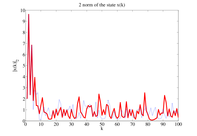
Figure 3. 2 norm of the state $x(k)$: proposed $\ell^{1}/\ell^{2}$ (solid) and conventional $\ell^{2}$ (dots)

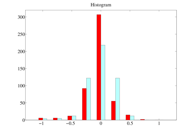
Figure 4. Histogram of the quantized values in all transmitted packets: proposed $\ell^{1}\!/\ell^{2}$ (left) and conventional $\ell^{2}$ (right)

To further investigate this issue, we compute the (discrete) entropy of the control values $\{u_{l}(k)\}$, defined as $\mathcal{H}(u)\triangleq-\sum_{u}\mathcal{P}(u)\log_{2}\mathcal{P}(u)$ [bits], where $\mathcal{P}(u)$ is the probability mass function of $u$; see, e.g., [6]. The function $\mathcal{P}(u)$ can be approximately estimated by the histogram as in Fig. 4. Note that here we do not take account of the entropy of control vector $U(k)$, that is, we assume scalar quantization. In the situation studied with $x(0)=[1,1,1,1]^{\top}$, the entropy by the $\ell^{1}\!/\ell^{2}$ optimization proposed is 8.6177, while that by the conventional $\ell^{2}$ approach is 9.5345. We next execute 10000 simulations with initial plant states $x(0)$ whose elements are randomly sampled from the Gaussian distribution with mean 0 and variance 1. The average entropies obtained are 12.2560 for $\ell^{1}\!/\ell^{2}$ optimization and 15.5701 for the $\ell^{2}$ formulation. Since the entropy of the signal transmitted serves as a measure of the code length, in the cases studied, the $\ell^{1}\!/\ell^{2}$ PPC method will require lower bit-rates than PPC with an $\ell^{2}$ cost function.

Fig. 5 illustrates the tradeoff between control performance and sparsity, which, as noted above, is related to bit-rates. The figure illustrates the average sparsity $5-\|U\|_{0}$, where

$$\|U\|_{0}\triangleq\frac{1}{100}\sum_{k=1}^{100}\|U(k)\|_{0},$$

and the achieved performance $\|x\|_{2}$ (the 2 norm of the state sequence $x$), for $\mu\in[0,100]$. The other parameters are the same as used above. As can be appreciated, as $\mu$ becomes larger, the sparsity increases, but the performance becomes worse.

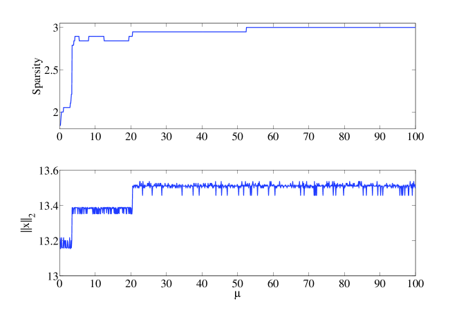
Figure 5. Sparsity $N-\|U\|_{0}$ (top figure) and performance $\|x\|_{2}$ (below), as a function of $\mu$.

6. Conclusion

We have studied a packetized predictive control formulation with an $\ell^{1}\!/\ell^{2}$ cost function. The associated optimization can be solved effectively and is, thus, suitable for implementation in a real-time controller. We have given sufficient conditions for practical stability when the controller is used over a network with bounded packet dropouts. Numerical results indicate that the proposed controller provides sparse control packets, thereby giving bit-rate reductions when compared to the use of, more common, quadratic cost functions. Future work may include the further study of performance aspects and the effect of plant disturbances.

References

• [1] A. Beck and M. Teboulle (2009), A fast iterative shrinkage-thresholding algorithm for linear inverse problems, SIAM J. Imaging Sciences, vol. 2, No. 1, pp. 183–202, 2009.
• [2] A. Bemporad (1998), Predictive control of teleoperated constrained systems with unbounded communication delays, IEEE CDC., pp. 2133–2138.
• [3] D. S. Bernstein (2005), Matrix Mathematics, Princeton University Press, 2005.
• [4] E. J. Candes and M. B. Wakin (2008), An introduction to compressive sampling, IEEE Signal Processing Magazine, vol. 25, pp. 21–30.
• [5] A. Casavola, E. Mosca, and M. Papini, Predictive teleoperation of constrained dynamic systems via Internet-like channels, IEEE Trans. Contr. Syst. Technol., vol. 14, no. 4, pp. 681–694.
• [6] T. M. Cover and J. A. Thomas (2006), Elements of Information Theory, 2nd Ed., Wiley-International.
• [7] I. Daubechies, M. Defrise, and C. De-Mol (2004), An iterative thresholding algorithm for linear inverse problems with a sparsity constraint, Commun. Pure Appl. Math., vol. 57, no. 11, pp. 1413–1457.
• [8] J. Fuchs (2004), On sparse representation in arbitrary redundant bases, IEEE Trans. Inform. Theory, vol. 50, no. 6, pp. 1341–1344.
• [9] G. C. Goodwin, M. M. Seron, and J. A. De Doná (2005), Constrained Control and Estimation, Springer.
• [10] S. S. Keerthi and E. G. Gilbert (1988), Optimal infinite-horizon feedback law for a general class of constrained discrete-time systems: stability and moving-horizon approximations, Journal of Optimization Theory and Applications, Vol. 57, No. 2, pp. 265–293.
• [11] M. Lazar (2009), Predictive Control Algorithms for Nonlinear Systems, Doctoral Thesis, Technical University of Iasi, Romana.
• [12] M. Lazar, W. P. M. H. Heemels, S. Weiland, and A. Bemporad (2006), Stabilizing model predictive control of hybrid systems, IEEE Trans. Automat. Contr., vol. 51, no. 11, pp. 1813–1818.
• [13] J. M. Maciejowski (2002), Predictive Control with Constraints, Pearson Education.
• [14] D. E. Quevedo and D. Nešić, Input-to-state stability of packetized predictive control over unreliable networks affected by packet-dropouts, IEEE Trans. Automat. Contr., Vol. 56, No. 2, pp. 370–375, 2011.
• [15] D. E. Quevedo and J. Østergaard and D. Nešić, Packetized predictive control of stochastic systems over bit-rate limited channels with packet loss, IEEE Trans. Automat. Contr., vol. 56, No. 11, 2011.
• [16] D. E. Quevedo, E. I. Silva, and G. C. Goodwin (2007), Packetized predictive control over erasure channels, Proc. Amer. Contr. Conf., pp. 1003–1008.
• [17] J. B. Rawlings and D. Q. Mayne (2009), Model Predictive Control Theory and Design, Nob Hill Publishing.
• [18] P. L. Tang and C. W. de Silva (2007), Stability validation of a constrained model predictive networked control system with future input buffering, Int. J. Contr., Vol. 80, No. 12, pp. 1954–1970.
• [19] K. Zhou, J. C. Doyle, and K. Glover (1996), Robust and Optimal Control, Prentice-Hall.
• [20] M. Zibulevsky and M. Elad (2010), L1-L2 optimization in signal and image processing, IEEE Signal Processing Magazine, Vol. 27, pp. 76–88.