.

SYSTEMATIC VARIATIONS
OF INTERSTELLAR LINEAR POLARIZATION AND
GROWTH OF DUST GRAINS

© 2013     N. V. Voshchinnikov^1,∗, H. K. Das², I. S. Yakovlev¹, V. B. Il’in^1,3,4

Submitted 21.02.2013

Abstract. A quantitative interpretation of the observed relation between the interstellar linear polarization curve parameters $K$ and $\lambda_{\max}$ characterizing the width and the wavelength of a polarization maximum, respectively, is given. The observational data available for 57 stars located in the dark clouds in Taurus, Chamaeleon, around the stars $\rho$ Oph and R CrA are considered. The spheroidal particle model of interstellar dust grains earlier applied to simultaneously interpret the interstellar extinction and polarization curves in a wide spectral range is utilized. The observed trend $K\approx 1.7\lambda_{\max}$ is shown to be most likely related to a growth of dust grains due to coagulation rather than mantle accretion. The relation of the parameters $K$ and $\lambda_{\max}$ with an average size of silicate dust grains is discussed.

Keywords: interstellar polarization — interstellar dust

……………………………..

^∗E-mail: nvv@astro.spbu.ru

INTRODUCTION

The interstellar (IS) polarization is a result of the linear dichroism of the interstellar medium which is caused by aligned nonspherical dust grains in the lines of sight. Extinction of the light by such particles depends on the orientation of the electric vector of the incident radiation. The linear polarization can be described by the polarization degree $P$ and the positional angle $\theta_{\rm E}$ ($\theta_{\rm G}$) measured in the equatorial (galactic) coordinate system. Historically, the direction of the IS polarization is related to the direction of the magnetic field component perpendicular to the line of sight.

Significant efforts were made to analyze the wavelength dependence of the IS polarization $P(\lambda)$. The polarization degree usually has a maximum in the visual and monotonically decreases to the ultraviolet and infrared (IR). Serkowski ([1973]) suggested an empirical formula to describe the dependence $P(\lambda)$ in the visual

$$P(\lambda)/P_{\max}=\exp[-K\ln^{2}(\lambda_{\max}/\lambda)].$$

Initially, this equation called Serkowski law was considered with two parameters: the maximum polarization wavelength $\lambda_{\max}$ and degree $P_{\max}$, while the parameter $K$ was taken to be constant equal to 1.15 (Serkowski, [1973]). This parameter determines the half-width of the normalized IS linear polarization curve

$$W=\lambda_{\rm max}/\lambda_{-}-\lambda_{\rm max}/\lambda_{+},$$

where $\lambda_{-}<\lambda_{\max}<\lambda_{+}$ and $P(\lambda_{+})=P(\lambda_{-})=P_{\max}/2$. The relation between $W$ and $K$ is as follows:

$$W=\exp[(\ln 2/K)^{1/2}]-\exp[-(\ln 2/K)^{1/2}].$$

Using the IR polarization data for 30 stars and considering $K$ as a free parameter, Wilking et al. ([1982]) found the correlation

$$K=(1.86\pm 0.09)\lambda_{\rm max}+(-0.10\pm 0.05).$$

Later Whittet et al. ([1992]) reconsidered this correlation utilizing the observations of 109 stars and obtained

$$K=(1.66\pm 0.09)\lambda_{\rm max}+(0.01\pm 0.05).$$ (1)

The linear function (1) well describes the general dependence of $K$ on $\lambda_{\max}$ derived for several dark clouds, but the observational data for some lines of sight can essentially differ from this dependence (Whittet et al., [1992]; Voshchinnikov, [2012]).

A qualitative explanation of the relation between the width of the IS polarization curve and the position of its maximum is connected to the growth of dust grains in the accretion and coagulation processes which lead to narrowing of the particle size distribution (see, e.g., Whittet et al., [1992]). The only attempt to quantitatively interpret the dependence $K$($\lambda_{\rm max}$) was made by Aannestad and Greenberg ([1983]) who considered effects of the ice mantle growth on cylindrical particles. This work has been criticized for a bad selection of the observational data and an incorrect calculation scheme (Mathis, [1986]; Voshchinnikov, [1989]; Whittet et al., [1992]).

In this work we model the dependence of $K$ on $\lambda_{\rm max}$ for a number of stars located in 4 dark clouds with different star formation activity. We use the model of spheroidal particles that was earlier applied to simultaneously interpret the IS extinction and polarization curves in a wide spectral range (Voshchinnikov and Das, [2008]; Das et al., [2010]).

OBSERVATIONAL DATA

We have selected the observational data available for the dark clouds in Taurus (14 stars), Chamaeleon (22 stars), around $\rho$ Oph (8 stars), and R CrA (13 stars). All the clouds are well-known sites of star formation (Mellinger, [2008]). They are situated in the local interstellar medium at the distance $D\approx 120-140$ pc from the Sun (Whittet et al., [1994], [2001]; Snow et al., [2008]; Peterson et al., [2011]). The clouds lie outside the Galaxy plane $|b|\mathrel{\mathchoice{\vbox{\offinterlineskip\halign{\hfil$\displaystyle#$\hfil\cr>\cr\sim\cr}}}{\vbox{\offinterlineskip\halign{\hfil$\textstyle#$\hfil\cr>\cr\sim\cr}}}{\vbox{\offinterlineskip\halign{\hfil$\scriptstyle#$\hfil\cr>\cr\sim\cr}}}{\vbox{\offinterlineskip\halign{\hfil$\scriptscriptstyle#$\hfil\cr>\cr\sim\cr}}}}12\hbox{${}^{\circ}$}$ and either belong to the Gould Belt or are close to it.

The observational data are collected in Tables 1–4 where one can find the name of the stars, their galactic coordinates, spectral type, visual extinction $A_{V}$ as well as the values of the Serkowski law parameters: $P_{\max}$, $\lambda_{\max}$, and $K$. The polarization data for the dark cloud in Taurus were taken from Efimov ([2009]) and Whittet et al. ([1992]), for thr dark cloud in Chamaeleon from Andersson and Potter ([2007]) and Whittet et al. ([2001]), for the dark cloud around $\rho$ Oph from Martin et al. ([1992]) and Wilking et al. ([1982]), and for the dark cloud around R CrA from Andersson and Potter ([2007]) and Whittet et al. ([1992]). Note that in all the clouds the positional angles are rather ordered. The stars selected are densely situated in the clouds in Chamaeleon and around R CrA and widely distributed (the angular distance between the stars may be of several degrees) in the clouds in Taurus and around $\rho$ Oph. The distances to the stars are mainly about 100–200 pc and only in a few cases reach 300–500 pc.

MODELLING

We represent the IS dust grains by homogeneous spheroids of different size and orientation. A solution to the light scattering problem for such particles has been given by Voshchinnikov and Farafonov ([1993]). To compare the theory and observations, one needs to calculate the intensity of radiation passed through an ensemble of partly aligned nonspherical particles. Such computations include two steps:

1. calculation of the polarization cross-sections $C_{\rm pol}=(C^{\rm TM}_{\rm ext}-C^{\rm TE}_{\rm ext})/2$, where the superscripts TM and TE denote two orthogonal cases of orientation of the electric vector of incident radiation (Bohren and Huffman, [1983]);

2. averaging of these polarization cross-sections over a given particle distribution over size and orientation.

Let us unpolarized stellar radiation passes through a dust cloud with the uniform magnetic field. As follows from observations and theoretical treatment (Dolginov et al., [1979]), the magnetic field determines the alignment of dust particles. The angle between the line of sight and the magnetic field is denoted by $\Omega$ ($0\hbox{${}^{\circ}$}\leq\Omega\leq 90\hbox{${}^{\circ}$}$). The linear polarization produced by rotating spheroidal particles in the line of sight is

$$P(\lambda)=\sum_{j}\int\limits_{0}^{D}\int\limits_{r_{V,\min,j}}^{r_{V,\max,j}}\overline{C}_{{\rm pol},j}(m_{\lambda,j},a_{j}/b_{j},r_{V},\lambda)\,n_{j}(r_{V})\,dr_{V}\,dl\times 100\,\%\,,$$

$$\overline{C}_{{\rm pol},j}={\frac{2}{\pi^{2}}}{\int\limits_{0}^{\pi/2}}{\int\limits_{0}^{\pi}}{\int\limits_{0}^{\pi/2}}\frac{1}{2}(C^{\rm TM}_{{\rm ext},j}-C^{\rm TE}_{{\rm ext},j})\,f_{j}(\xi,\beta,...)\,\cos 2{\psi}\,d{\varphi}\,d{\omega}\,d{\beta}\,,$$

where $D$ is the distance to the star, $\lambda$ the wavelength, $m_{\lambda,j}$, $a/b_{j}$ $n_{j}(r_{V})$ are the refractive index, aspect ratio and size distribution of spheroidal particles of the $j$th kind, $r_{V}$ is the radius of a sphere whose volume is equal to that of the spheroid (for prolate particles, $r_{V}=\sqrt[3]{ab^{2}}$, and for oblate ones, $r_{V}=\sqrt[3]{a^{2}b}$), ${r_{V,\min,j}}$ and ${r_{V,\max,j}}$ are the minimum and maximum radii, $C^{\rm TM,\,TE}_{{\rm ext},j}$ the extinction cross-sections for two polarization modes depending on the particle orientation, the angle $\psi$ can be expressed through $\varphi,\omega,\beta,\Omega$ (see the definitions of the angles and some relations between them, e.g., in Hong and Greenberg ([1980]) or Das et al. ([2010]), and finally ${f}_{j}(\xi,\beta,...)$ is the distribution of the particles of the $j$th kind over orientations.

We assume that the spheroidal grains are partly aligned so that their major axes rotate in a plane ($\varphi$ is the angle of rotation) and their angular momentum J precesses around the direction of the magnetic field ($\omega$ is the precession angle, $\beta$ the opening angle of the precession cone). Such alignment is called the imperfect Davis–Greenstein (IDG) alignment. It is described by the distribution function ${f}(\xi,\beta)$ depending only on the orientation parameter $\xi$ and the angle $\beta$.

It should be noted that the problem of dust grain orientation is the most complicated one in the physics of cosmic dust. In this problem the interactions of dust grains with gas, radiation and the magnetic fields are closely related. Davis and Greenstein ([1951]) suggested that the iron atoms included in dielectric dust grains made them paramagnetic, which gave the possibility of the grain interaction with a weak magnetic field. Alignment arises due to the paramagnetic relaxation of rotating dust grains. The Davis–Greenstein mechanism was further developed by Jones and Spitzer ([1967]) who obtained expressions for the angular momentum distribution function. In the simplest case this function is as follows:

$${f}(\xi,\beta)=\frac{\xi\sin\beta}{(\xi^{2}\cos^{2}\beta+\sin^{2}\beta)^{3/2}}.$$

The parameter $\xi$ depends on the particle size $r_{V}$, the imaginary part of the magnetic susceptibility of a dust grain $\chi^{\prime\prime}=\varkappa\omega_{\rm d}/T_{\rm d}$, where $\omega_{\rm d}$ is the angular velocity of the particle, gas density $n_{\rm g}$, magnetic field strength $B$, temperatures of dust $T_{\rm d}$ and gas $T_{\rm g}$

$$\xi^{2}=\frac{r_{V}+\delta_{0}(T_{\rm d}/T_{\rm g})}{r_{V}+\delta_{0}},$$

where

$$\delta_{0}^{\rm IDG}=8.23\,10^{23}\frac{\varkappa B^{2}}{n_{\rm g}T_{\rm g}^{1/2}T_{\rm d}}\,\mu{\rm m}.$$

If the particles are not aligned, we have $\xi=1$ and ${f}(\xi,\beta)=\sin\beta$. In the case of the perfect Davis–Greenstein (PDG) alignment $\xi=0$ and ${f}(\xi,\beta)=\delta(\beta)$, where $\delta(z)$ is the delta-function.

Different mechanisms of cosmic dust grain alignment have been extensively developed in the last few years (see discussion in Andersson ([2013]) and Voshchinnikov et al. ([2012])), but their role still remains unclear.

We selected the power-law size distribution of dust grains

$$n(r_{V})\propto r_{V}^{-q}\,$$ (2)

introduced by Mathis et al. ([1977]) from fitting the IS extinction data. This distribution has three parameters: the minimum ($r_{V,\min}$) and maximum ($r_{V,\max}$) size and the exponent $q$. Mathis et al. ([1977]) have reproduced the mean IS extinction curve using a mixture of graphite and silicate spheres with the parameters: $q=3.5$, $r_{V,\min}\approx 0.005\,\mu{\rm m}$ and $r_{V,\max}\approx 0.25\,\mu{\rm m}$.

The ensemble average size of dust grains $\langle r_{V}\rangle$ is defined as follows:

$$\langle r_{V}\rangle=\frac{\displaystyle\int\limits_{r_{{}_{V},\min}}^{r_{{}_{V},\max}}r_{V}n(r_{V})\,{d}r_{V}}{\displaystyle\int\limits_{r_{{}_{V},\min}}^{r_{{}_{V},\max}}n(r_{V})\,{d}r_{V}}\,.$$ (3)

In modelling we use the particles of the astronomical silicate (astrosil) and amorphous carbon (the BE type) whose refractive indices were taken from Draine ([2003]) and Zubko et al. ([1996]), respectively.

RESULTS AND DISCUSSION

From Figs. 1–4 (even despite the observational errors) one can see a clear correlation of the Serkowski law parameters $K$ and $\lambda_{\max}$ in all the clouds: $K$ increases (i.e. the width of the polarization curve $W$ decreases) with an increasing $\lambda_{\max}$. Slight doubt arises only in the case of the cloud around $\rho$ Oph where one star strongly affects the correlation coefficient (see Fig. 3).

To interpret the observations we used homogeneous spheroidal particles of astrosil and amorphous carbon. The prolate and oblate particles with the size $r_{V}=0.001-0.5\,\mu{\rm m}$ and the aspect ratio $a/b=1.5,2,3,4,5$ were utilized. Though the silicate and carbonaceous particles comparably contribute to extinction, the polarization is assumed to be produced only by silicate particles. Such an assumption has been earlier done by Chini and Krügel ([1983]) and Mathis ([1986]), and recently has got additional support in the work of Voshchinnikov et al. ([2012]) who found a correlation between the observed IS polarization degree and the abundance of silicon in dust grains.

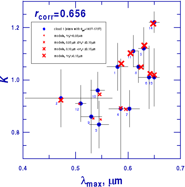
Figure 1: The Serkowski law parameter $K$ in dependence on the maximum polarization wavelength $\lambda_{\max}$. The points show the observational data (with their errors) for 14 stars in Taurus (the star numbers are as in Tabl. 1). The coefficient of correlation between $K$ and $\lambda_{\max}$ is $r_{corr}$. Crosses illustrate the results of modelling. The size of crosses is proportional to the mean size of silicate particles $\langle r_{\rm Si}\rangle$.

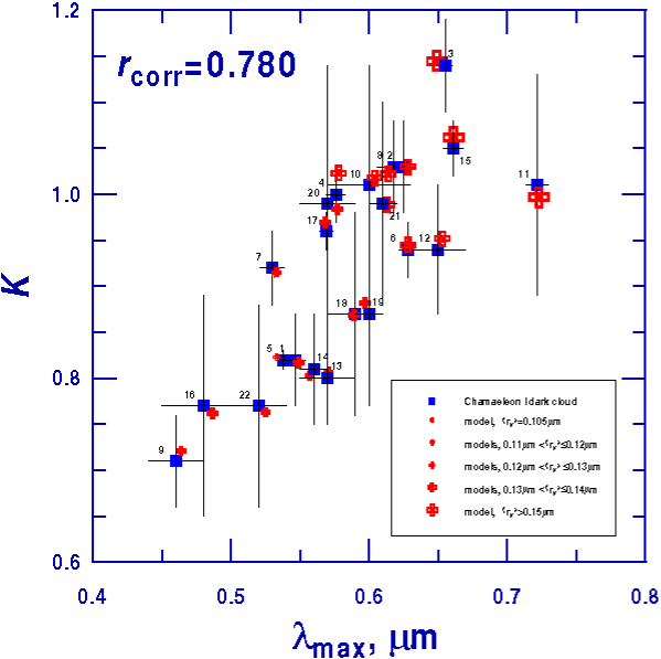
Figure 2: The same as in Fig. 1, but for 22 stars in the dark cloud in Chamaeleon (see Tabl. 2).

For each star in Tabl. 1–4, we have constructed a set of the models, calculated the Serkowski law parameters: $P_{\max}$, $\lambda_{\max}$, and $K$, and compared them with the observed value. In this paper the discussion is restricted by consideration of the relation between the width of the polarization curve and the position of its maximum. These characteristics of the Serkowski law are mainly determined by the parameters of the size distribution of silicate particles and weakly depend on the degree and direction of the particle orientation. This orientation is known to mainly affect the ratio $P_{\max}/A_{V}$ being the polarizing efficiency of the interstellar medium in a given direction. Therefore, the ratio $P_{\max}/A_{V}$ can be used to estimate the spacial structure of the magnetic fields in interstellar clouds (Voshchinnikov, [2012]).

For all stars, we found the models whose parameters $K$ and $\lambda_{\max}$ are close to the observed ones. These theoretical values of the parameters are represented by the cross size in Figs. 1–4. All the values agree with the observed ones within the errors. In these models we used spheroids with the aspect ratio $a/b=3$ or 4, other ratios gave similar results. Our search for the models reproducing the observational data was mainly performed by varying the parameters of the size distribution: $r_{V,\min}$, $r_{V,\max}$, and $q$. In this fitting we kept the total to selective extinction ratio $R_{V}=A_{V}/E(B-V)$ of our mixtures of silicate and carbonaceous particles within a reasonable interval.

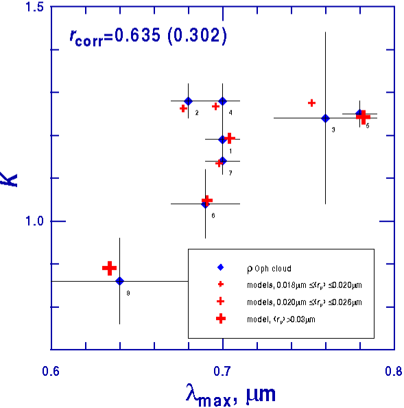
Figure 3: The same as in Fig. 1, but for 8 stars in the dark cloud around $\rho$ Oph (see Tabl. 3). The correlation coefficient $r_{corr}$ is computed for all stars (in brackets the coefficient for all stars without N 8).

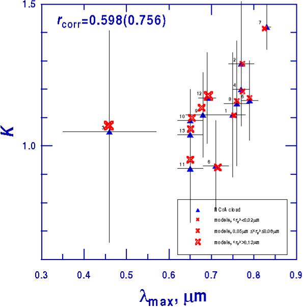
Figure 4: The same as in Fig. 1, but for 13 stars in the dark cloud around R CrA (see Tabl. 4). The correlation coefficient $r_{corr}$ is computed for all stars (in brackets the coefficient for all stars without N 22).

It should be noted that different values of the model parameters (e.g., those of the particle shape and of the size distribution) can give similar results — this point has been discussed by Das et al. ([2010]). However, in such cases the mean size of particles $\langle r_{V}\rangle$ weakly changes. So, it is a useful parameter to characterize the particle ensembles. The values of the mean size of silicate particles $\langle r_{\rm Si}\rangle$ in the successful models are presented in the last column of Tabl. 1–4.

Already the first look at the tables leads to the conclusion that there is no correlation between visual extinction $A_{V}$ and the mean size of silicate particles $\langle r_{\rm Si}\rangle$. The same is correct when we consider the mean size of both silicate and carbonaceous particles. However, this cannot be considered as an argument against the growth of dust grains in the dense parts of the clouds. It rather argues for inhomogeneous structure of the clouds and the presence of extended regions of low density in the lines of sight.

The mean size of interstellar dust grains is thought to be changed mainly by the following processes:

1. Accretion of gas atoms on dust grains. In this case the growth rate is not assumed to depend on the particle size (Greenberg, [1968]; Voshchinnikov, [1986]). So, an increase of the minimum and maximum sizes of dust grains occurs with the exponent being constant, i.e. $r_{V,\min}$ grows, $r_{V,\max}$ grows, and $q=$ const. with time.

2. Destruction of smaller dust grains, e.g. because of their evaporation close to hot objects. Here we have an increase of the minimum size only or in other words the size distribution becomes narrower, i.e. $r_{V,\min}$ grows, $r_{V,\max}=$ const., and $q=$ const. with time.

3. Coagulation due to grain-grain collisions. In this case the exponent changes (the size distribution becomes more flat), i.e. $r_{V,\min}=$ const., $r_{V,\max}=$ const., and $q$ decreases with time.

The scheme described is very simplified, but it is suitable for understanding of the main effects produced by the dust grain growth processes mentioned. In particular, it is easy to see that grain coagulation should lead to an anticorrelation of the parameters $q$ and $\langle r_{\rm Si}\rangle$, while two other processes should cause a correlation between $r_{V,\min}$ and $\langle r_{\rm Si}\rangle$. These dependencies are presented in Figs. 5 and 6.

From Fig. 5 one can see that the grain growth due to coagulation may take place in all the clouds but with a different efficiency. The growth due to accretion may occur in the cloud in Taurus (see Fig. 6).

Our results show that the mean size of particles producing the linear polarization in the clouds around $\rho$ Oph and R CrA is essentially smaller than that in the clouds in Taurus and Chamaeleon. It can be seen in Figs. 1–4 where the size of crosses presenting the theoretical results is proportional to the mean size of particles. Note a different position of the regions of smaller and larger values of $\langle r_{\rm Si}\rangle$ in the figures: small crosses concentrate in the left bottom quarter for the clouds in Taurus and Chamaeleon and in the right upper quarter for the clouds around $\rho$ Oph and R CrA. For the large crosses, the situation is opposite. It should be noted that there are stars in the clouds around $\rho$ Oph and R CrA with $\lambda_{\max}>0.7\,\mu{\rm m}$, while for other two clouds usually $\lambda_{\max}\mathrel{\mathchoice{\vbox{\offinterlineskip\halign{\hfil$\displaystyle#$\hfil\cr<\cr\sim\cr}}}{\vbox{\offinterlineskip\halign{\hfil$\textstyle#$\hfil\cr<\cr\sim\cr}}}{\vbox{\offinterlineskip\halign{\hfil$\scriptstyle#$\hfil\cr<\cr\sim\cr}}}{\vbox{\offinterlineskip\halign{\hfil$\scriptscriptstyle#$\hfil\cr<\cr\sim\cr}}}}0.7\,\mu{\rm m}$. Besides that for some stars with large values of $\lambda_{\max}$ the IS polarization curve is very narrow (the values of $K$ are very large, see Figs. 3, 4).

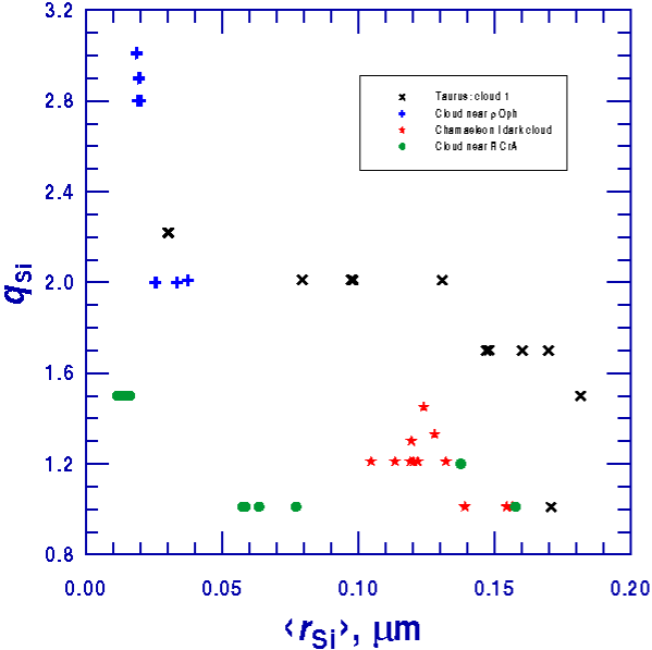
Figure 5: The exponent $q_{\rm Si}$ of the silicate particle size distribution in dependence on the mean size $\langle r_{\rm Si}\rangle$. The values of $q_{\rm Si}$ and $\langle r_{\rm Si}\rangle$ are obtained from fitting of the observational data for all 57 stars under consideration.

It is interesting to consider the dependence between the parameter $K$ or $\lambda_{\max}$ found by fitting and the mean size of particles. The dependence of $K$ on $\langle r_{\rm Si}\rangle$ is shown in Fig. 7, $\lambda_{\max}$ depends on $\langle r_{\rm Si}\rangle$ in a similar way. Both dependencies have non-monotonous character (see Fig. 7). The polarization curve reaches a maximum width (the minimum value of $K$) for $\langle r_{\rm Si}\rangle\approx 0.10\,\mu{\rm m}$. With a growing mean size of particles, the curve $P(\lambda)$ becomes more narrow and $\lambda_{\max}$ increases. However, the extreme values of $\lambda_{\max}$ and $K$ can be also explained using rather small particles. Generally, the dependence of $K$ on $\langle r_{\rm Si}\rangle$ or $\lambda_{\max}$ on $\langle r_{\rm Si}\rangle$ can be described by a parabola (see Fig. 7), which does not correspond to the simple linear function (see, e.g., Whittet, [2003])

$$\lambda_{\max}\approx 2\pi\langle r\rangle(n-1),$$

where $n$ is the real part of the refractive index.

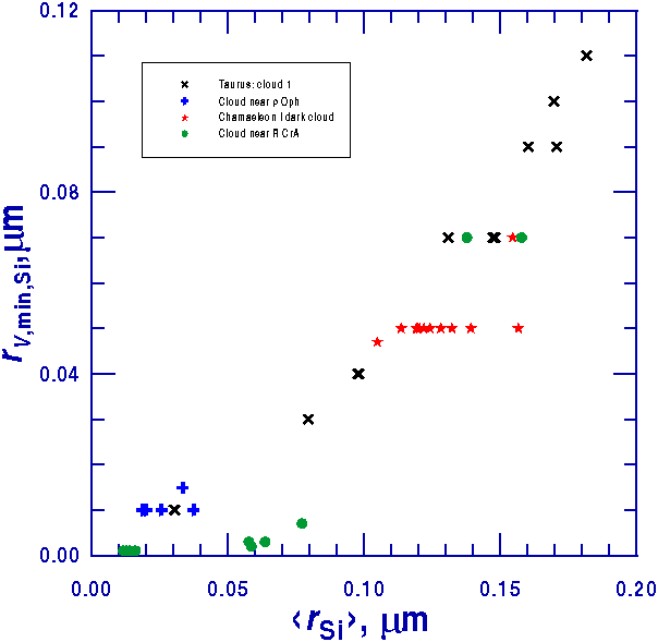
Figure 6: The same as in Fig. 5, but for the relation between the minimum $r_{V,\min,\rm Si}$ and mean $\langle r_{\rm Si}\rangle$ sizes of silicate particles.

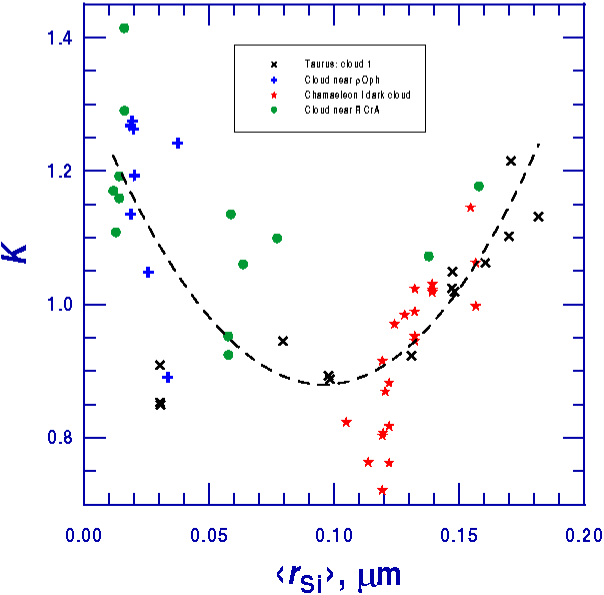
Figure 7: The Serkowski law parameter $K$ in dependence on the mean size of silicate particles $\langle r_{\rm Si}\rangle$. The values of $K$ and $\langle r_{\rm Si}\rangle$ were obtained from fitting the data for 57 stars. The dotted line shows the approximation of the dependence of $K$ on $\langle r_{\rm Si}\rangle$ by a quadric polynomial.

The polarization data for the clouds around $\rho$ Oph and R CrA can be reproduced if one uses the particle ensembles with $q\mathrel{\mathchoice{\vbox{\offinterlineskip\halign{\hfil$\displaystyle#$\hfil\cr<\cr\sim\cr}}}{\vbox{\offinterlineskip\halign{\hfil$\textstyle#$\hfil\cr<\cr\sim\cr}}}{\vbox{\offinterlineskip\halign{\hfil$\scriptstyle#$\hfil\cr<\cr\sim\cr}}}{\vbox{\offinterlineskip\halign{\hfil$\scriptscriptstyle#$\hfil\cr<\cr\sim\cr}}}}0$ (see Fig. 8). In the figure we present the data for all 57 stars under consideration. The theoretical dependencies show changes of the Serkowski law parameters when only accretion (for the mechanism 2, the situation is similar) or coagulation (the mechanism 3) occurs. The model with the parameters: $a/b=3$ (prolate spheroids), $r_{V,\min}=0.07\,\mu{\rm m}$, $r_{V,\max}=0.35\,\mu{\rm m}$, and $q=2$ was selected as a basic model. As follows from Fig. 8, coagulation of dust grains leads to a monotonous growth of $K$ and $\lambda_{\max}$, but at the same time the wavelength dependence of extinction $A(\lambda)$ becomes less selective and the ratio $R_{V}$ increases up to very high values. Considering the accretion process, one should pay attention to the non-monotonous character of the dependence of $K$ on $\lambda_{\max}$, i.e. similar polarization curves can be derived for quite different particle ensembles. Another interesting feature of the accretion mechanism is that for a fixed $q$ one cannot obtain the values of $\lambda_{\max}$ below some limit value (e.g., for $q=2$ we got $\lambda_{\max}\mathrel{\mathchoice{\vbox{\offinterlineskip\halign{\hfil$\displaystyle#$\hfil\cr>\cr\sim\cr}}}{\vbox{\offinterlineskip\halign{\hfil$\textstyle#$\hfil\cr>\cr\sim\cr}}}{\vbox{\offinterlineskip\halign{\hfil$\scriptstyle#$\hfil\cr>\cr\sim\cr}}}{\vbox{\offinterlineskip\halign{\hfil$\scriptscriptstyle#$\hfil\cr>\cr\sim\cr}}}}0.51\,\mu{\rm m}$). Obviously, the possibility of using smaller particles to interpret the data for stars with very large values of $\lambda_{\max}$ needs further analysis and discussion. Another way to solve the problem of very narrow $P(\lambda)$ curves is to apply a mixture of particles of quite different shapes.

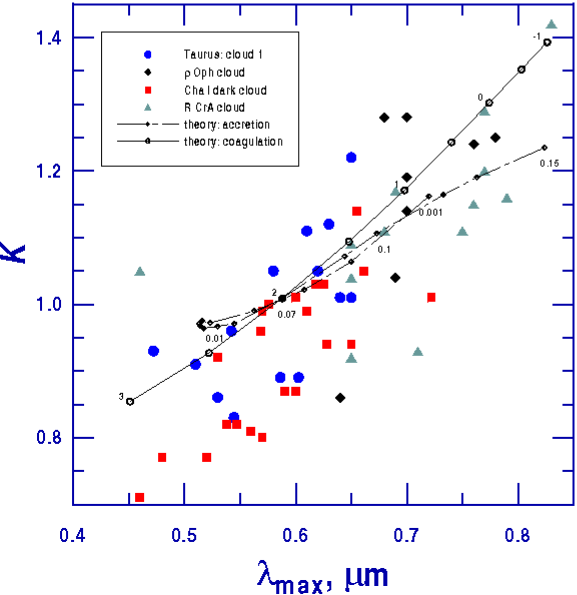
Figure 8: The parameter $K$ in dependence on $\lambda_{\max}$. The filled signs show the observational data (without observational errors) for 57 stars. The empty signs correspond to results of calculations when the grain growth due to accretion (squares) or coagulation (circles) takes place. The numbers close to these signs show the values of the exponent $q_{\rm Si}$ or the minimum size $r_{V,\min,\rm Si}$. The calculations were performed for the angle between the line of sight and the magnetic field direction $\Omega=60\hbox{${}^{\circ}$}$.

CONCLUSIONS

For 57 stars in 4 dark clouds with different star formation activity, we have modeled the observed wavelength dependencies of the linear polarization degree $P(\lambda)$ described by the Serkowski law parameters $P_{\max},\lambda_{\max}$ and $K$. Polarization in the model was produced by an ensemble of homogeneous silicate spheroidal particles with a power-law size distribution and imperfect Davis–Greenstein alignment.

For all the stars we found the size distribution parameters giving the observed values of $P_{\max},\lambda_{\max}$, and $K$. Analysis of the results obtained has shown that the dust grain growth can occur in all the clouds under consideration, but with different efficiency. The growth caused by accretion may take place only in the cloud in Taurus.

It is shown that in most of the cases the dust grain ensembles can be characterized by the only parameter — the mean size of particles. We have considered the relation between the parameters $\lambda_{\max}$, $K$ and the mean size of silicate particles $\langle r_{\rm Si}\rangle$. It is found that narrow red-shifted polarization curves $P(\lambda)$ observed for some stars can be explained by larger or smaller particles, i.e. by using ensembles with a larger or smaller value of $\langle r_{\rm Si}\rangle$. These results require a special discussion with regard to the properties of individual clouds that will be done in a separate paper.

The work was partly supported by the grant of Russian Foundation for Basic Researches 11-02-92695-IND-a.

REFERENCES

Table 1. Stars in the cloud 1 in Taurus

$N$	Star	$l$	$b$	Sp.Type	$A_{V}$	$P_{\max},\,\%$	$\lambda_{\max}$, $\mu{\rm m}$	$K$	$\langle r_{\rm Si}\rangle$, $\mu{\rm m}$
1	HD 28225	170.74	–14.35	A3 III	1.22	1.88	0.58	1.05	0.1604
2	HD 29835	174.14	–12.86	K2 III	1.20	4.06	0.472	0.93	0.1309
3	HD 30168	174.76	–12.44	B8 V	1.02	4.08	0.545	0.83	0.0305
4	HD 283637	170.51	–14.84	A0 V	2.28	2.73	0.586	0.89	0.0976
5	HD 283642	171.55	–15.35	A3 V	2.19	2.01	0.63	1.12	0.1817
6	HD 283643	171.83	–15.07	A2 V	1.66	1.35	0.64	1.01	0.1471
7	HD 283701	172.18	–13.63	B8 III	2.53	3.20	0.603	0.89	0.0982
8	HD 283757	174.01	–14.81	A5 V	1.65	2.92	0.62	1.05	0.1471
9	HD 283800	173.57	–12.29	B5 V	1.64	3.95	0.53	0.86	0.0303
10	HD 283812	174.90	–13.07	A1 V	1.92	6.26	0.542	0.96	0.0795
11	HD 283815	175.32	–13.90	A5 V	1.91	2.86	0.61	1.11	0.1698
12	HD 283855	174.25	–11.47	A2	1.99	5.13	0.51	0.91	0.0303
13	HD 283877	174.94	–12.72	F5 V	0.72	1.65	0.65	1.01	0.1481
14	HD 283879	175.72	–12.61	B5 V	3.33	4.24	0.65	1.22	0.1707

Table 2. Stars in the dark cloud Chamaeleon I

$N$	Star	$l$	$b$	Sp.Type	$A_{V}$	$P_{\max},\,\%$	$\lambda_{\max}$, $\mu{\rm m}$	$K$	$\langle r_{\rm Si}\rangle$, $\mu{\rm m}$
1	Cha F1	296.05	–15.70	K4 III	0.8	3.35	0.547	0.82	0.1219
2	Cha F2	296.65	–16.60	B8 V	1.8	3.85	0.625	1.03	0.1392
3	Cha F3	296.26	–15.84	B4 V	2.4	5.45	0.655	1.14	0.1545
4	Cha F6	296.39	–15.48	A2 V	1.6	5.48	0.576	1.00	0.1322
5	Cha F7	296.28	–15.24	B5 V	1.7	5.92	0.538	0.82	0.1048
6	Cha F9	296.66	–15.62	K0 III	2.5	4.82	0.628	0.94	0.1322
7	Cha F11	296.53	–15.06	B9 V	2.9	4.81	0.530	0.92	0.1192
8	Cha F16	296.99	–15.74	G2 IV	3.1	7.30	0.618	1.03	0.1392
9	Cha F21	296.83	–15.29	K3 III	2.2	5.41	0.46	0.71	0.1192
10	Cha F25	297.13	–15.54	G8 III	5.4	8.01	0.60	1.01	0.1392
11	Cha F28	297.24	–15.73	K4 III	6.1	7.02	0.722	1.01	0.1566
12	Cha F29	297.28	–15.74	K6	2.7	5.05	0.65	0.94	0.1322
13	Cha F30	297.04	–15.13	K3 III	1.9	4.41	0.57	0.80	0.1195
14	Cha F32	296.98	–14.80	A7 V	2.2	2.34	0.56	0.81	0.1192
15	Cha F36	297.47	–15.73	K0 III	5.7	12.19	0.661	1.05	0.1566
16	Cha F39	297.49	–15.20	K3 III	0.9	3.22	0.48	0.77	0.1219
17	Cha F40	297.69	–15.64	B8 III	2.1	8.01	0.569	0.96	0.1241
18	Cha F41	296.88	–13.48	B8 V	0.9	2.60	0.59	0.87	0.1203
19	Cha F42	297.08	–13.61	A3/A4 IV	1.2	2.87	0.60	0.87	0.1219
20	Cha F48	297.56	–14.07	B9.5 V	0.6	2.29	0.57	0.99	0.1281
21	Cha F52	297.77	–13.91	B9.5 V	1.2	2.99	0.61	0.99	0.1322
22	Cha F54	298.17	–14.17	G6 III/IV	0.8	2.68	0.52	0.77	0.1136

Table 3. Stars in the dark cloud around $\rho$ Oph

$N$	Star	$l$	$b$	Sp.Type	$A_{V}$	$P_{\max},\,\%$	$\lambda_{\max}$, $\mu{\rm m}$	$K$	$\langle r_{\rm Si}\rangle$, $\mu{\rm m}$
1	HD 145502	354.61	+22.70	B2IV	1.06	1.25	0.70	1.19	0.0201
2	HD 147084	352.33	+18.05	A4II/III	2.70	4.42	0.68	1.28	0.0197
3	HD 147283	352.29	+17.61	A1IV	2.53	1.61	0.76	1.24	0.0192
4	HD 147888	353.65	+17.71	B3V:SB	2.08	3.63	0.70	1.28	0.0187
5	HD 147889	352.87	+17.04	B2V	4.44	4.02	0.78	1.25	0.0375
6	HD 147932	353.72	+17.71	B5V	2.10	3.11	0.69	1.04	0.0256
7	HD 147933	353.68	+17.70	B1.5V	2.07	2.69	0.70	1.14	0.0187
8	HD 150193	355.60	+14.83	A1Ve	1.79	5.10	0.64	0.86	0.0335

Table 4. Stars in the dark cloud around R CrA

$N$	Star	$l$	$b$	Sp.Type	$A_{V}$	$P_{\max},\,\%$	$\lambda_{\max}$, $\mu{\rm m}$	$K$	$\langle r_{\rm Si}\rangle$, $\mu{\rm m}$
1	RCrA 12	359.46	–18.65	G8III	1.7	0.81	0.75	1.11	0.0126
2	RCrA 15	359.65	–18.66	G1	1.1	3.00	0.77	1.29	0.0161
3	RCrA 22	000.10	–18.09	K5III	3.3	1.30	0.46	1.05	0.1377
4	RCrA 28	000.12	–17.59	M5III	1.3	2.10	0.77	1.20	0.0141
5	RCrA 30	359.52	–18.04	A0V	2.6	1.85	0.79	1.16	0.0116
6	RCrA 43	359.49	–17.25	K0III	1.9	1.73	0.71	0.93	0.0577
7	RCrA 46	359.65	–17.56	G8III	3.3	2.71	0.83	1.42	0.0161
8	RCrA 50	359.44	–17.37	A6V	1.3	1.11	0.76	1.15	0.0141
9	RCrA 52	359.44	–17.32	G5III	1.6	1.99	0.68	1.11	0.0586
10	RCrA 56	000.29	–18.68	G5IV	1.9	2.08	0.65	1.09	0.0772
11	RCrA 58	359.41	–17.90	K1III	2.3	0.80	0.65	0.92	0.0577
12	RCrA 71	000.11	–18.84	F6V	1.3	1.03	0.69	1.17	0.1578
13	RCrA 73	000.10	–19.04	G0V	1.2	1.80	0.65	1.04	0.0636

REFERENCES

- 1983 Aannestad, P.A., and J.M. Greenberg (1983) Astrophys. J. 272, 551.
- 2013 Andersson, B.-G. (2012) Magnetic Fields in Diffuse Media (Ed. A. Lazarian, E.M. de Gouveia Dal Pino, Berlin: Springer), in press (astro-ph 1208.4393).
- 2007 Andersson, B.-G., and S.B. Potter (2007) Astrophys. J. 665, 369.
- 1983 Bohren, C.F., and D.R. Huffman (1983) Absorption and Scattering of Light by Small Particles (NY: J.Wiley & Sons).
- 1983 Chini, R., and E. Krügel (1983) Astron. Astrophys. 117, 289.
- 2010 Das, H.K., N.V. Voshchinnikov, and V.B. Il’in (2010) MNRAS 404, 265.
- 1951 Davis, L., and J.L. Greenstein (1951) Astrophys. J. 114, 206.
- 1979 Dolginov, A.Z., Yu.N. Gnedin, and N.A. Silant’ev (1979) Propagation and Polarization of Radiation in Cosmic Medium (Moscow, Nauka).
- 2003 Draine, B.T. (2003) Astrophys. J. 598, 1026.
- 2009 Efimov, Yu.S. (2009) Bull. CrAO 105, 126.
- 1968 Greenberg, J.M. (1968) Interstellar Grains, In Stars and Stellar Systems, Vol. VII, ed. B.M. Middlehurst and L. H. Aller, Univ. Chicago Press, p. 221
- 2012 Hirashita, H. (2012) MNRAS 422, 1263.
- 1980 Hong, S.S., and J.M. Greenberg (1980) Astron. Astrophys. 88, 194.
- 1967 Jones, R.V., and L. Spitzer (1967) Astrophys. J. 147, 943.
- 1992 Martin, P.G., A.J. Adamson, D.C.B. Whittet, et al. (1992) Astrophys. J. 392, 691.
- 1986 Mathis, J.S. (1986) Astrophys. J. 308, 281.
- 1977 Mathis, J.S., W. Rumpl, and K.H. Nordsieck (1977) Astrophys. J. 217, 425.
- 2008 Mellinger, A. (2008) Handbook of Star Forming Regions, vol. 1 (Ed. B. Reipurth, San Francisco: Astron. Soc. Pacific), p. 1.
- 2011 Peterson, D.E., A. Caratti o Garatti, T.L. Bourke, et al. (2011) Astrophys. J. Suppl. 194, 43.
- 1973 Serkowski, K. (1973) Interstellar Dust and Related Topics, IAU Symp. 52 (Ed. J.M. Greenberg, D.S. Hayes, Dordrect: Reidel), p. 145.
- 2008 Snow, T.P., J.D. Destree, and D.E. Welty (2008) Astrophys. J. 679, 512.
- 1986 Voshchinnikov, N.V. (1986) Interstellar Dust, (Moscow: VINITI), in Russian.
- 1989 Voshchinnikov, N.V. (1989) Astron. Nachr. 310, 265.
- 2012 Voshchinnikov, N.V. (2012) J. Quant. Spectrosc. Radiat. Transfer 113, 2334.
- 2008 Voshchinnikov, N.V., and H.K. Das (2008) J. Quant. Spectrosc. Radiat. Transfer 109, 1527.
- 1993 Voshchinnikov, N.V., and V.G. Farafonov (1993) Astrophys. Space Sci. 204, 19.
- 2012 Voshchinnikov, N.V., Th. Henning, M.S. Prokopjeva, and H.K. Das (2012) Astron. Astrophys. 541, A52.
- 2003 Whittet, D.C.B. (2003) Dust in the Galactic Environments (Bristol: Inst. Phys. Publ.).
- 1992 Whittet, D.C.B., P.G. Martin, J.H. Hough, et al. (1992) Astrophys. J. 386, 562.
- 1994 Whittet, D.C.B., P.A. Gerakines, A.L. Carkner, et al. (1994) MNRAS 268, 1.
- 2001 Whittet, D.C.B., P.A. Gerakines, J.H. Hough, et al. (2001) Astrophys. J. 547, 872.
- 1982 Wilking, B.A., M.J. Lebofsky, and G.H. Rieke (1982) Astron. J. 87, 695.
- 2008 Zhukovska, S., H.-P. Gail, and M. Trieloff (2008) Astron. Astrophys. 479, 453.
- 1996 Zubko, Z.V., V. Mennella, L. Colangeli, and E. Bussoletti (1996) MNRAS 282, 1321.