Switching of anisotropy and phase diagram
of a Heisenberg square lattice $S=1/2$ antiferromagnet Cu(pz)₂(ClO₄)₂.

Abstract

Experiments in the antiferromagnetic phase of a quasi 2D $S=1/2$ quasi-square lattice antiferromagnet Cu(pz)₂(ClO₄)₂ reveal a biaxial type of the anisotropy, instead of the easy-plane one, considered before. The weak in-plane anisotropy, found by means of electron spin resonance spectroscopy and magnetization measurements, is about an order of magnitude weaker, than the off-plane anisotropy. The weak in-plane anisotropy results in a spin-flop phase transition for the magnetic field aligned along easy axis, and, thereby, in a bicritical point on the phase diagram. A remarkable feature of the weak in-plane anisotropy is the abrupt change of its sign at the spin-flop point. This anisotropy switching disappears at the tilting of magnetic field to the easy axis by the angle of 10^∘ within the plane. The nature of the abrupt anisotropy reversal remains unclear. The phase diagram is characterized by the increase of the ordering temperature $T_{N}$ in the magnetic field used, except for a dip near the bicritical point.

I Introduction

Heisenberg $S=1/2$ antiferromagnet on a square lattice (HSLAF) is a popular model of low-dimensional magnetismManousakis (1991). An ideal HSLAF has no long-range order except at $T=0$, where a Néel-type ground state with 40% reduction of ordered spin component should be realizedWhite and Chernyshev (2007). In real quasi-2D antiferromagnet a weak interlayer interaction is present, providing a Néel order at $T>0$. An organometallic compound Cu(pz)₂(ClO₄)₂ (copper pyrazine perchlorate) has been considered as an example of quasi-2D HSLAF: copper ions carrying spin $S=1/2$ are bridged together in a slightly distorted square lattice layers by pyrazine (C₄H₄N₂) rings as shown on Fig. 1.

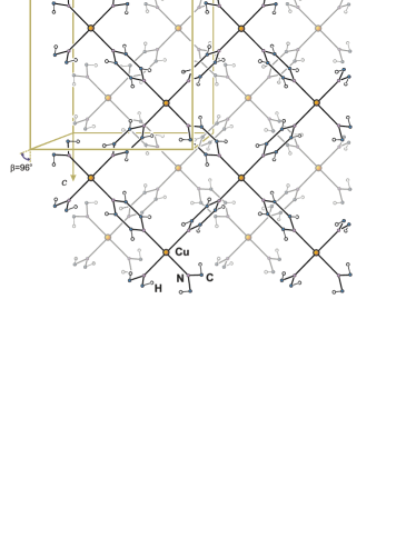
Figure 1: (Color online) Cu(pz)₂(ClO₄)₂ structure. Two layers, each containing a square magnetic lattice, are displayed; ClO₄ complexes are not shown for clarity. Colors of ions and connecting lines in the lower layer are faded out. Crystallographic data are taken from [Woodward et al., 2007].

Copper pyrazine perchlorate crystallizes from a solution in the space group $C2/m$ at room temperature, however, at cooling, near 180 K, there is a phase transition to a structure which has the space group $C2/c$ [Woodward et al., 2007]. In the low temperature phase, parameters $b$ and $c$ of the monoclinic lattice are close to each other. The rectangles with sides $b$ and $c$ are approximately squares. Diagonals of these rectangles form a rhombic lattice, these rhombuses are slightly distorted squares. The angle between the $a$ and $c$ axes differs only a little from $90^{\circ}$, thus the lattice may be represented as weakly distorted tetragonal lattice. Magnetic ions Cu²⁺ ($S$=1/2), placed at the corners of rhombuses, form layers in $bc$ planes. The nearest neighbor exchange paths are symmetrically equivalent and exactly identical. Therefore the exchange network within the $bc$ planes is equivalent to that of a square lattice. Due to ClO₄ complexes between the layers, they are well separated, as well as due to half a period in-plane shift between layers. Because of this shift a magnetic ion within a layer is equidistant from four ions in adjacent layer, therefore the interlayer coupling is canceled in the first orderWoodward et al. (2007).

Indeed, estimation of the interlayer effective exchange $J_{\perp}$ from values of $T_{N}=4.25$ K and nearest-neighbor exchange $J=18.1$ K by an empirical relation $J_{\perp}/J\sim\exp{(-\frac{2.3J}{T_{N}})}$ derived from quantum Monte-Carlo simulationYasuda et al. (2005), leads to a very small value of $J_{\perp}\simeq 9\cdot 10^{-4}J$ [Lancaster et al., 2007]. Magnetic moment per Cu²⁺ ion in the two sublattice structure is only $0.47\mu_{B}$ at $T\rightarrow 0$ in zero field, as detected by elastic neutron scatteringTsyrulin et al. (2010). This quantum spin reduction indicates strong influence of quantum fluctuations on the ground state. From the observation of increase of ordered spin component in external field Tsyrulin et alTsyrulin et al. (2010) conclude, that the fluctuations are suppressed by magnetic field. A related evidence of fluctuations suppression is the significant growth of $T_{N}$ in magnetic field, confirmed by neutron scattering and specific heat measurementsTsyrulin et al. (2010). A gap of $E_{0}\simeq 0.2$ meV in the spin-wave spectrum, detected by inelastic neutron scatteringTsyrulin et al. (2010, 2010), was ascribed to easy-plane ($XY$-type) anisotropy, keeping the spins within the $bc$ plane. The observation of minimum in susceptibility vs temperature dependence for a field directed perpendicular to $bc$ plane is consistent with quantum Monte-Carlo (QMC) simulationsCuccoli et al. (2003), which predict the minimum of the susceptibility for HSLAF with a small $XY$ anisotropy.

We describe systematic investigations of Cu(pz)₂(ClO₄)₂ by means of multifrequency electron spin resonance (ESR) spectroscopy and magnetization measurements for different orientations of magnetic field. Our main result is the observation and measurement of a weak in-plane anisotropy, not detected in previous measurements. This weak anisotropy induces remarkable features of the phase diagram. These are i) the spin-flop phase transition in a magnetic field applied along the easy axis, ii) a bicritical point and iii) a dip in $T_{N}(H)$ dependence near the bicritical point. From antiferromagnetic resonance spectrum we also find that the weak in-plane anisotropy is surprisingly changing its sign by a jump at the spin-flop point. Besides, this effect of abrupt anisotropy reversal arises as another phase transition at tilting the magnetic field, at a critical angle between the magnetic field and the easy axis.

II Experiment

Samples of Cu(pz)₂(ClO₄)₂ have been grown in Clark University as described in [Woodward et al., 2007]. The lattice parameters of the monoclinic $C2/c$ lattice are $a=14.072(5)$, $b=9.786(3)$ and $c=9.781(3)$ Å; $\beta=96.458(4)^{\circ}$. Crystals are flat rectangular plaquettes colored blue, of the typical size of 2x2 mm²; the plane of square lattice ($bc$ plane) coincides with the plane of the plaquette. Sides of square crystal plaquettes are aligned at $45^{\circ}$ to $b$ and $c$ axes, coinciding with the directing lines of magnetic square lattice, see a sketch on margins of Fig.4.

ESR experiments were performed in Kapitza Institute, using a set of resonator spectrometric inserts in ⁴He pumping cryostat with a cryomagnet. The frequency range from $5$ to $140$ GHz was covered. A spectrometric insert for $18-140$ GHz range has a rotable sample holder, allowing to change the orientation of the sample with respect to magnetic field during the experiment. A small amount of DPPH, free radical compound with $g=2.00$, was used as a magnetic field labelPoole (1983).

Magnetization experiments were performed at the Department of Low Temperature Physics and Superconductivity of M. V. Lomonosov Moscow State University on Quantum Design 9 Tesla PPMS machine equipped with vibrating sample magnetometer (VSM) and at the Neutron Scattering and Magnetism Group in the Laboratory for Solid State Physics at ETH Zürich with the identical machine. The lowest available temperature was 1.8 K.

III ESR data

III.1 Temperature evolution of ESR signal

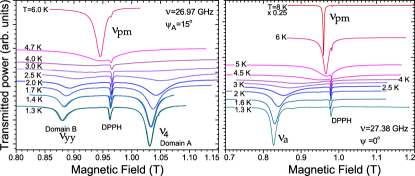
Figure 2: (Color online) Left panel: resonance line temperature evolution in a sample, containing two types of domains, when $\psi_{A}=15^{\circ}$. Right panel: resonance line temperature evolution in single domain sample when $\psi=0^{\circ}$. In both cases $\xi=0^{\circ}$, i. e. field lies in $xy$ plane. The angles $\psi$ and $\xi$ are defined on Fig.4. A scaling factor of 0.25 is applied to 8 K line on the right panel.

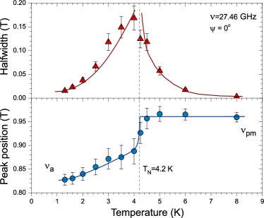
Figure 3: (Color online) Changes of resonance field and linewidth through $T_{N}$ in a single domain sample for $\mathbf{H}\parallel x$ at $\nu=27.46$ GHz; corresponding set of ESR signals is shown at the right panel of Fig. 2. Lines are guide to the eye.

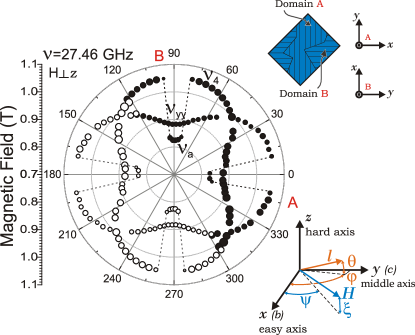
Figure 4: (Color online) Polar plot of $27.46$ GHz ESR field at rotating Cu(pz)₂(ClO₄)₂ sample in the $bc$ plane; $T=1.3$ K. Solid symbols correspond to actual experimental data, and open symbols are the repetition of solid symbols with the 180^∘ period. Symbols size corresponds to resonance intensity. Dashed lines are guide to an eye. A rough sketch of a two-domain sample and orientation of $x$,$y$,$z$ axes within domains is shown.

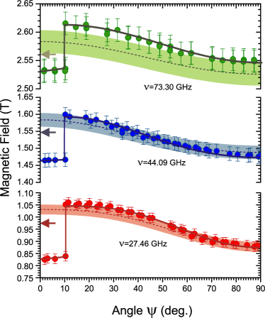
Figure 5: (Color online) Summary of angular dependencies in $xy$-plane for a domain. Solid lines are guide for the eye, dashed lines are theoretical calculation (biaxial model) with a shaded region around, marking a possible error due to the parameters uncertainty. Arrows indicate the field of paramagnetic resonance at corresponding frequency.

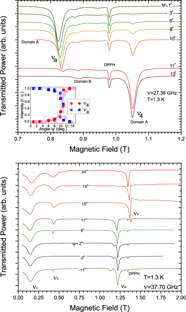
Figure 6: (Color online). Evolution of the ESR line of a single domain sample at the rotation of the magnetic field within the $xy$-plane near the critical angle $\psi_{c}=10^{\circ}$, when regular mode $\nu_{4}$ transforms to anomalous mode $\nu_{a}$. Zero field cooling from 15 K to $T=1.3$ K was performed before each record. Upper panel: $\nu=27.28$ GHz. Lower panel: $\nu=37.7$ GHz. Inset: Angular dependences of the intensities of ESR modes $\nu_{4}$ (red circles) and $\nu_{a}$ (blue squares). Each half-open symbol corresponds to a line recorded after zero-field cooling. Solid symbols present ESR lines recorded without thermocycling, each rotation performed in a field 1.2 T. Thick lines are guide for an eye.

Magnetic resonance signal in Cu(pz)₂(ClO₄)₂ at temperatures above $T_{N}=4.2$ K corresponds to a typical exchange-narrowed paramagnetic resonance of Cu²⁺ ions with anisotropic $g$–factor. The values of $g$–factor, obtained by high-temperature ($T\gtrsim 10$ K) ESR measurements are $g_{x}=g_{y}=2.05$ and $g_{z}=2.28$. A narrow Lorentzian line, with a halfwidth of about $5\cdot 10^{-3}$ T, broadens with cooling, and becomes unresolvable near $T_{N}$. Below $T_{N}$ the ESR response becomes strongly anisotropic. For ${\bf H}\parallel z$ a broad signal transforms into a single narrow line, shifted from high-temperature position, while for ${\bf H}\parallel x,y$ two lines appear, as shown on left panel of Fig. 2. The resonance halfwidth shows a clear critical dependence near the phase transition temperature. The divergency in the line halfwidth together with the shift of the resonance position, as shown on Fig. 3, can be used as a marker of phase transition, allowing us to extract $T_{N}$ from the ESR data. The value of $T_{N}$=4.2$\pm 0.1$ K is in agreement with the results of magnetization measurements, as shown on the phase diagram (Fig. 16).

III.2 Antiferromagnetic resonance

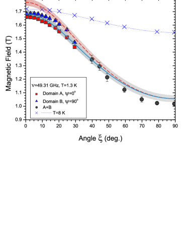
Figure 7: (Color online) Angular dependence of the field of $49.31$ GHz ESR in a two-domain sample of Cu(pz)₂(ClO₄)₂ at the temperature $T=1.3$ K. Rotation is performed in the xz-plane of the domain A. Triangles — domain A, squares – domain B, circles – signal of the whole sample when domains become indistinguishable, crosses – $T=8$ K ). Solid line presents the calculated low-temperature resonance field (biaxial model)for $\psi=90^{\circ}$, dashed line - for $\psi=0$ and dotted line - theory for high-temperature paramagnetic resonance. Shaded region marks error boundaries of model calculation (see text).

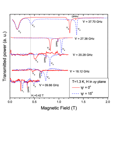
Figure 8: (Color online) Collection of ESR lines at $T=1.3$ K for fields along $\psi=0^{\circ}$ (red solid) and $\psi=15^{\circ}$ (blue dashed). Vertical dashed line denotes critical field $H_{c}=0.42$ T at this temperature.

The anisotropy within the $bc$ plane below $T_{N}$ results in the angular dependence of the resonance field, as shown on Figs. 4, 5. This reveals two kinds of resonances with the identical rosette-like angular dependencies, which are shifted for 90^∘ on Fig. 4. The relation between the intensities of these two kinds of signals is different for different samples. This observation indicates a presence of two kinds of domains. The ratio of intensity of signals from two kinds of domains has the same value for zero-field cooling and field-cooling of the sample in the field of 6 T, as well as at thermocycling through $T_{N}$. Therefore we conclude, that these domains are crystallographic domains, for which $b$ axes are rotated for 90^∘. We denote domains with orthogonal $b$ ($c$) axes as domain A and domain B. One of the samples has the intensity for one rosette much stronger than for another one. For this, approximately single domain sample, the relation between the volumes of domains of different types may be evaluated, e.g., from the relation of intensities of ESR lines presented on Fig.6, upper panel, between 0.82 and 0.88 T. Such an estimation gives the number of spins, belonging to domain A, approximately 30 times greater than to domain B. This sample remained approximately a single domain one at numerous cycles of cooling from the room temperature.

The rosettes shown on Fig.4 demonstrate a smooth evolution of the resonance field with the angle in the whole angle range except for the narrow range in the vicinity of $b$-direction. This direction was identified for the nearly single domain sample by room temperature X-ray diffraction. At the angle $\psi=10^{\circ}$ there is a step-like jump of the resonance field, shown in Fig.4 and Fig. 5. Near the exact orientation of the external field along $b$-axis, i.e. when tilting $\psi$ does not exceed 10^∘, the resonance field is shifted to much lower field and this position can not be extrapolated from the smooth angular dependence in the main part of the field range. Therefore we denote the resonance observed at $\mid\psi\mid<10^{\circ}$ as anomalous mode $\nu_{a}$. The redistribution of the intensity from the regular to the anomalous mode at a slow rotation of the field is shown on Fig. 6. One can see here that the transmission of the intensity between the two types of resonances has a character of a switching, it is performed within an interval of about 1^∘ which may be a measure of the mosaic of the sample. Thus, a narrow phase transition at the angle variation is observed.

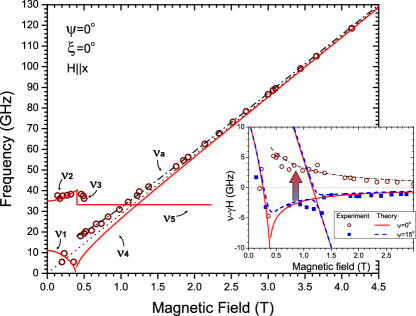
Figure 9: (Color online) AFMR spectra at $T=1.3$ K for field along easy axis. Solid line is the model calculation, dash-dotted line is the empirical formula (1). Insert: shift from paramagnetic resonance frequency vs. field for directions $\psi=0^{\circ}$ (empty circles) and $\psi=15^{\circ}$ (solid squares) in $xy$ plane. Solid and dashed lines are theoretical calculations, corresponding to these cases. Dash-dotted line is the same, as on main plot.

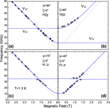
Figure 10: (Color online) AFMR spectra for several field directions in $xy$ plane and along $z$ axis at $T=1.3$ K. Solid lines are calculation according to (21) with $\Delta_{y}=11$ GHz and $\Delta_{z}=35$ GHz, dashed lines are paramagnetic resonance with $g_{xy}=2.05$ and $g_{z}=2.28$.

We didn’t observe any difference between the resonance signals, indicating this transition, when passing the critical angle in a field or in zero-field, and for passing the critical angle at the temperature above or below $T_{N}$. Tilting the field within the $xz$-plane conserves the anomalous mode, as shown on Fig. 7, at least in the range $\mid\xi\mid\lesssim 30{{}^{\circ}}$, where the difference between the anomalous mode and an extrapolation for a regular mode may be detectable. The anomalous mode was observed only at $\mu_{0}H>0.4$ T. Below this field the resonance positions at $\psi=0^{\circ}$ and $\psi=15^{\circ}$ are almost identical, as one can see on upper and lower records of Fig.8 and on the low-field part of frequency-field dependencies on the inset of Fig. 9. At the same time, at $\mu_{0}H>0.4$ T there is a jump-like evolution of the resonance field and frequency in this range of angles.

Further, we measured ESR fields for a set of frequencies (see examples of records on Fig.8) at three principal directions of the magnetic field and at a tilting angle $\psi=15^{\circ}$, as well as for two intermediate orientations in $bc$ plane. The corresponding frequency-field dependencies are presented on Figs. 9,10. From these data we conclude, that the spectrum of frequencies of the antiferromagnetic resonance has two energy gaps, approximately equal to 35 and 10 GHz and two branches in a magnetic field. For the direction of the magnetic field near $b$-axis there is a mode softening at approaching the field of 0.42 T from the zero-field side. At $\mu_{0}H>0.42$ T we observe the softened mode in the angular range of the regular mode and the anomalous mode in the narrow angle range $\mid\psi\mid<10^{\circ}$. By changing the angle $\psi$ across the critical value toward $\psi=0$, the ESR frequency is transposed from the value below the paramagnetic resonance frequency $g_{x}\mu_{B}\mu_{0}H/2\pi\hbar$ to the value above it. This transposition is marked by an arrow on the inset of Fig. 9, it occurs by a jump at crossing the critical angle $\psi_{c}=10^{\circ}$. This jump corresponds exactly to the jump of the resonance field, shown on Fig. 5.

We note here that the observed frequency-field dependencies for field orientation in the whole solid angle, except for the range of the anomalous mode, may be well described by the calculated frequencies of the two sublattice antiferromagnet with a biaxial anisotropy and the easy axis directed along $b$, see, e.g. Ref.Nagamiya et al., 1955. The calculated frequencies are given in the Appendix A and presented on Figs. 9, 10 by solid lines. Eight curves shown here, and the calculated angular dependencies shown on Fig. 7 are parameterized only by two energy gaps and three $g$-factors. The $g$-factors $g_{x}$, $g_{y}$, $g_{z}$ are measured independently in the paramagnetic phase and are not fitting parameters. Below the critical field of 0.42 T, the frequencies in the whole solid angle range of the magnetic field directions are described with that model. In particular, a mode softening at ${\bf{H}}\parallel b$ indicates the spin-flop transition. By this observation we can conclude that $b$ is the easy axis direction. For the anomalous mode, observed at $\mid\psi\mid<10^{\circ}$, $\mid\xi\mid<30^{\circ}$, $\mu_{0}H>0.42$ T we use the empirical relation

$$\nu_{a}=\sqrt{\Delta_{a}^{2}+(\frac{g_{x}\mu_{B}}{2\pi\hbar}\mu_{0}H)^{2}}$$ (1)

with $\Delta_{a}=14$ GHz at $T=1.3$ K. This relation represents the observed frequency at the unexpected position above (and not below) the paramagnetic resonance frequency at $H>H_{c}$.

Thus, the ESR data reveal a weak magnetic anisotropy in $bc$ plane and a spin-flop transition, as well as the anomalous mode $\nu_{a}$ appearing in the narrow angular range of the field direction instead of a regular resonance of a biaxial antiferromagnet.

IV Magnetization

IV.1 Field along the easy axis

The main feature of low-temperature magnetization curves at ${\bf H}\parallel b$ is the presence of jump in magnetization corresponding to the spin-flop transition, detected by ESR. As it is shown at Fig. 11, magnitude of the jump increases with cooling, and its position shifts to lower fields. Jump in magnetization disappears around $4\pm 0.05$ K, which is lower than $T_{N}$. The sharp increase in magnetization can also be seen in $M(T)$ curves, present on Fig. 12. Crossing the spin-flop phase boundary by temperature in a constant field also gives a very pronounced step in magnetic moment. This step disappears at $\mu_{0}H=0.74$ T, and above this field there appears a minimum on the $M$ $vs$ $T$ dependence. Below the temperature of the minimum of the magnetization there is a kink, marking the onset of long range order. The minimum and the kink are marked on Fig. 12. Both minimum and kink shift upwards in temperature with increasing field up to 9 T, though the former becomes less pronounced. Note, that there is no offset on Fig. 12, and stacking of the curves reflects the nonlinearity of magnetization process.

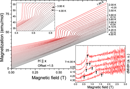
Figure 11: (Color online) Isothermal low-field magnetization curves of Cu(pz)₂(ClO₄)₂, field along $x$. An offset of $1.5$ emu/mol per curve is present. Upper insert: an expanded region around the temperature, where magnetization jump disappears. Lower insert: a few $dM/dH$ curves are shown, allowing to locate phase transitions between disordered and ordered phases, marked by arrows.

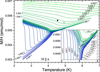
Figure 12: (Color online) Normalized magnetization $M(T)/H$ for various magnetic fields, directed along $x$. Insert: an expanded region around the point, where magnetization jump vanishes.

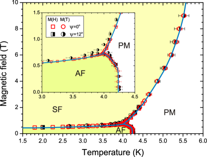
Figure 13: (Color online) Phase diagram of Cu(pz)₂(ClO₄)₂, field along easy axis. AF is $\mathbf{l}\parallel x$ collinear antiferromagnetic phase, SF is spin-flop antiferromagnetic phase and PM is paramagnetic phase. Circles are features in $M(T)$ curves, squares are features in $M(H)$; red points correspond to $\psi=0^{\circ}$ orientation, and black — to $\psi=12^{\circ}$. Lines are guide for an eye. In the insert an expanded region around the bicritical point is shown.

We derive the ordering point by a peak in the derivative $\partial(MT)/\partial T$, as suggested by FisherFisher (1962). We can also detect this transition by a peak in the derivative $dM/dH$ of isothermal magnetization curve, as displayed at the insert of Fig. 13. A final phase diagram, with points on phase boundaries obtained by both $M(T)$ and $M(H)$ scans, is present at Fig. 13.

IV.2 Field in $bc$ plane

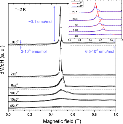
Figure 14: (Color online) Magnetization derivative $dM/dH$ for various directions of magnetic field in $xy$ plane at $T=2$ K. Dashed lines show zero for corresponding curves. Inset: temperature dependencies of magnetization derivatives for directions $\psi=8^{\circ}\pm 2^{\circ}$ and $\psi=10^{\circ}\pm 2^{\circ}$.

On Fig. 14 a collection of magnetization derivatives $dM(H)/dH$ for various directions of magnetic field in $xy$ plane is present. $dM(H)/dH$ curves show a sharp peak at $\psi\rightarrow 0$, which broadens with misalignment. Left wing of the peak is always smooth, in contrast to a discontinuity in the right wing of the peak. The discontinuity exists up to a critical angle $\psi_{c}$, observed in angular dependences of ESR, see Figs. 4, 5. When tilt angle exceeds $\psi_{c}$, the $dM/dH$ curve becomes completely smooth. The transition between smooth and discontinuous types of derivative, which affects mostly the right wing, occurs abruptly. This difference between the curves, corresponding to field tilts below and above $\psi_{c}$, is pronounced in a whole temperature range where spin-flop transition takes place, as shown in the inset of Fig. 14. The discontinuity of differential susceptibility $dM/dH$ occurs exactly at the same magnitude and in the same angular range $\mid\psi\mid<\psi_{c}$, as the anomalous ESR mode $\nu_{a}$.

With further increase in $\psi$ peak becomes less pronounced and almost disappears when $\psi$ approaches $\sim 45^{\circ}$. Magnetization curve at $\sim 45^{\circ}$ (this is the direction along natural crystal facets) doesn’t show a step, and demonstrates a smooth slope increase, as observed in Ref. Xiao et al., 2009.

We have also performed a study of a phase diagram with magnetic field, slightly tilted from $x$ axis. The orientation we chose was $\psi=12\pm 2^{\circ}>\psi_{c}$. Here Cu(pz)₂(ClO₄)₂ still demonstrates increase in magnetization near $H_{c}$, but the transition is regular, i.e. with a smooth derivative $dM/dH$ on both sides of $H_{c}$. We locate $H_{c}$ and $T_{N}$ in the same way as was described before for ${\bf H}\parallel x$. The resulting phase boundaries are also shown at Fig. 13, and the difference between phase diagram for exact and misaligned orientations along $x$ is observed only near the bicritical point.

IV.3 Field along middle and hard axes

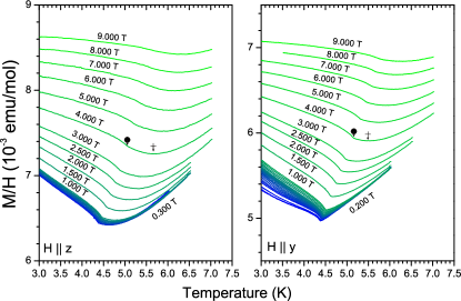
Figure 15: (Color online) Normalized magnetization $M(T)/H$ for various magnetic fields, directed along $z$ (left panel) and $y$ (right panel). Values of magnetic field between $0.3$ and $1$ Tesla are the same, that on Fig. 12. The kink and the minimum on the curves are marked by a droplet and a cross, respectively.

Curves of normalized magnetization for the fields, directed along middle axis $y$ and hard axis $z$ at Fig. 15 don’t show spin-flop, but demonstrate an increase of $T_{N}$ in a magnetic field. The only qualitative difference between this two sets of curves is in the onset of minimum of $M(T)$: for field along $y$ the minimum appears for the applied fields between $1.5$ and $2$ T, while for field along $z$ it is present even at $H\rightarrow 0$ (as independently confirmed by zero-field ac magnetization measurementsXiao et al. (2009)). Another feature of $M(T)$ curves at ${\bf H}\parallel y$ is the existence of inflection point below $T_{N}$ at low fields, in contrast to the case of ${\bf H}\parallel z$. As the field is increased, the inflection disappears.

V Discussion

V.1 Biaxial model and spectra

In section III we have presented AFMR spectra for various field directions. These spectra follow biaxial collinear antiferromagnet paradigm for all magnetic field directions, except for a small solid angle corresponding to anomalous mode. The anomalous mode is observed in a solid angle of about of $10^{-2}4\pi$, close to easy axis, and only above $H_{c}$. Resonance frequencies in this range of fields and angles correspond to a gapped branch (1) with $\Delta_{a}=14$ GHz. This unexpected effect can be described as an in-plane anisotropy switching caused by spin flop, i.e. the resonant frequencies are that of a two sublattice biaxial antiferromagnet, for which $x$ turns abruptly from the easy- into middle axis and $y$ turns into easy axis at the spin-flop point. This conclusion is made on the base of the experimental observation of the anomalous mode, which appears at $H>H_{c}$ and has the frequency following the relation (A3), corresponding to middle axis orientation of the field, instead of expected (A7), derived for the easy axis orientation.

We consider the magnetoelastic hypothesis, which might explain the switching of anisotropy at the spin flop point. The in-plane anisotropy, marking the easy axis, originates from rhombic distortion of square lattice, for Cu(pz)₂(ClO₄)₂ this distortion is due to a relative difference of about $\sim 10^{-4}$ between the lattice constants $b$ and $c$. In principle, the antiferromagnetic ordering may cause a striction of the same order of magnitudeMorosin (1970). Because of the magnetostriction, the in-plane anisotropy may be dependent on the magnitude and the direction of sublattice magnetizations, and, therefore, it should change when the spin flop transition takes place. One could expect the $y$ axis to become easy axis, and $x$ to become middle axis immediately after the spin-flop.

Nonetheless, a simple quantitative formulation of this approach, described in details in Appendix B, does not capture a step-like angular dependence of AFMR field in $xy$-plane, and is in a contradiction with the observed relation between the zero-field gap and a critical field. The analysis of a complete Lagrangian, allowed by symmetry, should include several dozens of magnetoelastic and elastic terms and was not performed.

Another possibility, presumably explaining the nature of anomalous mode $\nu_{a}$, is the existence of a phase, other than collinear for $H>H_{c},\psi<\psi_{c}$. This implies destabilizing of collinear phase by frustration when external field compensates in-plane anisotropy. However, our measurements do not support this hypothesis: magnetization curve $M(H)$ and phase boundary $T_{N}(H)$ are indistinguishable for $\psi<\psi_{c}$ and $\psi>\psi_{c}$ in fields above $H_{c}$.

The influence of a change of the direction and magnitude of zero point fluctuations at the spin flop may be also of importance, because anisotropic spin fluctuations also contribute to the energy of anisotropy.

Nevertheless, the nature of the anisotropy switching remains unclear.

To give a connection with the previous work [Tsyrulin et al., 2010] we derive a relation between zero-field gaps $\Delta_{y,z}$ of antiferromagnetic resonance and the parameters of microscopic model Hamiltonian. In nearest-neighbor exchange approximation the complete biaxial Hamiltonian reads as

$${\widehat{\mathcal{H}}}=\sum\limits_{\langle i,i^{\prime}\rangle}J\widehat{\mathbf{S}}_{i}\widehat{\mathbf{S}}_{i^{\prime}}-g\mu_{B}\mu_{0}\sum\limits_{i}\mathbf{H}\widehat{\mathbf{S}}_{i}$$ (2)

$$\phantom{HHH}-\sum\limits_{\langle i,i^{\prime}\rangle}\left(\delta J_{y}\widehat{S}^{y}_{i}\widehat{S}^{y}_{i^{\prime}}+\delta J_{z}\widehat{S}^{z}_{i}\widehat{S}^{z}_{i^{\prime}}\right),$$

where $\delta J_{y}$ and $\delta J_{z}$ are parameters of so-called ’exchange anisotropy’. According to linear spin-wave approximation, which have proven to be good for describing the $k$-dependence of the spectrum in the vicinity of Brillouin zone center of Cu(pz)₂(ClO₄)₂ [Tsyrulin et al., 2010], the energy gaps are related to exchange anisotropy parameters as

$$\Delta_{y,z}=2\sqrt{2J\delta J_{y,z}}.$$ (3)

In this spin-wave approximation the sublattice magnetization is supposed to be $\mu_{B}$ per magnetic ion, which is not the case of the Cu(pz)₂(ClO₄)₂, where a strong quantum reduction of about 50 $\%$ is observed. A finer estimation for the case of $S=1/2$ SLAFM, considering $1/S$ corrections, was given by Weihong et alWeihong et al. (1991):

$$\Delta_{y,z}\simeq 1.2\sqrt{2J\delta J_{y,z}}.$$ (4)

Thus, this equation may be used for an estimation of $\delta J_{y,z}$. Spectroscopic gaps of $35\pm 2$ and $11\pm 2$ GHz are $\Delta_{z}=1.68\pm 0.1$ K and $\Delta_{y}=0.53\pm 0.1$ K correspondingly. Hence, from (4) we extract $\delta J_{z}=53.2$ mK and $\delta J_{y}=5.3$ mK. This corresponds to relative exchange anisotropy $\delta J_{z}/J=3.1\cdot 10^{-3}$ and $\delta J_{y}/J=3.1\cdot 10^{-4}$. This is in agreement with previous neutron data, except for the parameter $\delta J_{y}$, which was not resolved by neutron scattering experiment. We can characterize the observed anisotropy switching, in terms of changing of parameters of Hamiltonian (2). It corresponds to transformation of $\delta J_{y}$ into $\delta J_{y}^{\ast}$, which is of negative sign and equals $-6.7$ mK.

V.2 Phase diagrams

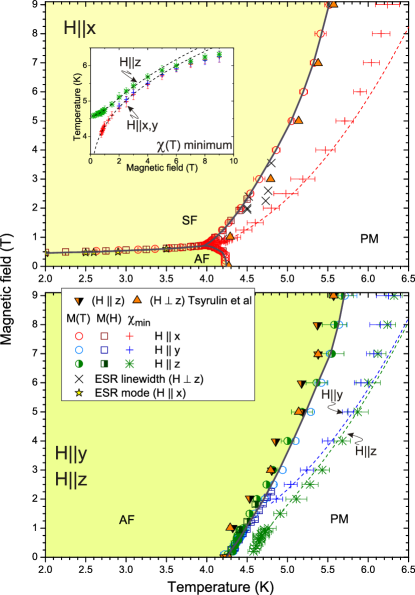
Figure 16: (Color online) Phase diagrams for $H\parallel x$ (upper panel) and $H\parallel yz$ (lower panel) directions. Points are experimental data: circles for $M(T)$ and squares for $M(H)$ features. Stars and diagonal crosses mark phase transitions determined by ESR, solid triangles are data from [Tsyrulin et al., 2010]. Horizontal crosses ($x$, $y$) and snowflakes ($z$) are minima in $M(T)$. Solid lines are guide for the eye, dashed lines are fit (5) for $T_{min}(H)$ The fit for all three orientations is separately shown in the insert in the upper panel.

Phase diagrams for $x$, $y$ and $z$ directions of magnetic field are present at Fig. 16. For $y$ and $z$ directions the phase diagram are analogous, with monotonous increase of $T_{N}$. For field along $x$ phase diagram is more complicated, with a bicritical point, where spin-flop, ordered and paramagnetic phases meet. The phase diagram presents the spin flop transition and the bicritical point in addition to the phase boundaries reported in the previous work using neutron scattering and specific heat measurementsTsyrulin et al. (2010).

The field, at which the antiferromagnetic resonance mode $\nu_{3}$ is observed, also marks the spin-flop transition (see Appendix). From ESR experiment we get $\mu_{0}H_{c}^{ESR}=0.45$ T at $T=1.3$ K (see Fig. 9), this field increases with temperature. Temperature dependence of $H_{c}$ derived from ESR is consistent with the magnetization measurements as shown on Fig. 16.

Minima of $M(T)$ are also plotted, showing different behavior for all three directions. While for ${\bf H}\parallel z$ minimum persists up to $H=0$ limit, for different directions it appears only at some finite field, at which $T_{min}$ reaches $T_{N}$.

The reason of this minimum may be qualitatively explained by the following consideration: for an easy-pane antiferromagnet it is natural to have an anisotropic susceptibility, which is larger for out-of-plane direction. In case of 2D antiferromagnet with $\delta J_{z}\ll J$ one should expect this anisotropic behavior to rise only at low temperatures, when $T<J$. Numerical simulations of HSLAF with a weak easy-plane anisotropyCuccoli et al. (2003) show, that tendency for increase of magnetization at $\bf{H}||z$ due to the onset of planar correlations overcomes the tendency for its decrease due to short-range AF order. Thus a characteristic minimum in $\chi(T)$ marks a crossover from Heisenberg to $XY$ behavior. Cuccolli et al Cuccoli et al. (2003), using a QMC data analysis, suggested a formula for estimation of $T_{min}$ in a case of easy-plane HSLAF model,

$$T_{min}=\dfrac{4\pi\rho_{s}}{\ln\left(\frac{C}{\delta_{eff}}\right)}.$$ (5)

Here $\rho_{s}\simeq 0.22J$ is the renormalized spin stiffness, $\delta_{eff}$ is the relative anisotropy and $C\simeq 160$ is the dimensionless constant. It has also been found, that presence of external magnetic field in 2D magnets makes them effectively easy-plane and induces both Berezinsky-Kosterlitz-Thouless transition at finite temperature and a minimum in $\chi(T)$ above it [Cuccoli et al., 2003]. In absence of long-range order, when a local order parameter $\mathbf{l}$ is formed, the orientation $\mathbf{l}\perp\mathbf{H}$ provides an energy gain. Hence, the short-range order parameter becomes 2D instead of 3D in the isotropic case and the effective anisotropy energy in this field-induced $XY$ behaviour is proportional to $H^{2}$ .

For the orientation of the magnetic field $\mathbf{H}\perp z$ for a strong enough field ($g\mu_{B}\mu_{0}H\gtrsim\sqrt{\delta J_{z}J}$), we consider ’effective’ easy-plane anisotropy induced by an external field. The easy plane of this anisotropy is perpendicular to the field. We take this anisotropy in the form derived in Ref. Cuccoli et al., 2003 for HSLAFM

$$\delta_{eff}^{xy}=\beta\left(\dfrac{g_{xy}\mu_{B}\mu_{0}H}{k_{B}J}\right)^{2},$$ (6)

where $\beta$ is a dimensionless parameter. Here we disregard smaller anisotropy $\delta J_{y}$, as the experimental $T_{min}(H)$ in $x$ and $y$ directions is the same within the error bars.

For the case $\mathbf{H}\parallel z$ the easy-plane anisotropy originates due to the combination of the natural and field-induced anisotropy. We empirically combine these two factors which were analyzed separately in QMC simulationsCuccoli et al. (2003, 2003)

$$\delta_{eff}^{z}=\dfrac{\delta J_{z}}{J}+\beta\left(\dfrac{g_{z}\mu_{B}\mu_{0}H}{k_{B}J}\right)^{2}.$$ (7)

Fitting experimental data for $T_{min}$ with equation (5), where $\delta_{eff}$ is set as $\delta^{xy}_{eff}$, or $\delta^{z}_{eff}$, and parameters $J=18.1$ K and $C=160$ are fixed, we yield $\rho_{s}\simeq 0.24J$, $\delta J_{z}\simeq 0.023$ K and $\beta\simeq 0.1$, which is quite close to the result of Cucolli et al [Cuccoli et al., 2003]. Fits are shown on Fig. 16 with dashed lines. This result can be considered as another indication of the 2D correlations developing in Cu(pz)₂(ClO₄)₂ at $T>T_{N}$. Nonetheless, value of $\delta J_{z}$ obtained by this fit is in better agreement with estimation by Eq. 3, which does not take into account quantum renormalization of the gap, than with Eq. 4, which considers $1/S$ corrections.

For ${\bf H}\parallel x$ (i.e. field along the easy axis) there is a bicritical point $(H_{c},T_{c})$. Three phase transition lines meet in this point: second order paramagnetic to collinear antiferromagnetic phase transition (PM-AF), second order paramagnetic to flopped antiferromagnetic phase transition (PM-SF) and first order spin-flop phase transition AF-SF. In the vicinity of bicritical point the following scaling equations are expectedKosterlitz et al. (1976): for AF-SF transition temperature dependence for critical field is

$$H^{2}(T)-H_{c}^{2}=A\left(\frac{T}{T_{c}}-1\right),$$ (8)

while for ordering transitions to AF and SF phases relations between magnetic field and ordering temperatures are

$$H^{2}(T)-H_{c}^{2}=A\left(\frac{T}{T_{c}}-1\right)-B_{AF}\left(\frac{T}{T_{c}}-1\right)^{\phi}$$ (9)

and

$$H^{2}(T)-H_{c}^{2}=A\left(\frac{T}{T_{c}}-1\right)+B_{SF}\left(\frac{T}{T_{c}}-1\right)^{\phi}$$ (10)

correspondingly. For ’classical’ 3D antiferromagnet scaling exponent is known to be $\phi=1.25$ for uniaxial and $\phi=1.175$ for biaxial anisotropy. Theory also suggests amplitude ratio $Q=B_{SF}/B_{AF}=1$ for the former caseKosterlitz et al. (1976); King and Rohrer (1979). In contrast, for pure 2D case with easy-axis anisotropy bicritical point is expectedNelson and Pelcovits (1977); Kosterlitz and Santos (1978); Cowley et al. (1993) to occur only at $T=0$ — a simple argument for that is the following: when easy-axis anisotropy is compensated by the external field, the system becomes equivalent to non-perturbed two-dimensional Heisenberg model, which can possess long-range order only at zero temperature. The PM-AF and PM-SF phase boundaries, which meet at $T=0$, are defined by

$$|H^{2}(T)-H_{c}^{2}|\propto T^{-2}\exp\left(-\frac{4\pi\rho_{s}}{T}\right).$$ (11)

The above equation is valid only in the absence of additional anisotropies and interlayer couplings, while in case of Cu(pz)₂(ClO₄)₂ both of these perturbations are present and the bicritical point is at $T>0$. A numerical proof for the latter statement can be found, e.g., in Monte-Carlo study of classical anisotropic $XY$ antiferromagnet on square lattice [Holtschneider and Selke, 2007], where the phase diagram strongly resembles that of a 3D easy-axis AFM. Hence, phase diagram of Cu(pz)₂(ClO₄)₂ turns out to be an intermediate case between ideal 2D and conventional 3D anisotropic antiferromagnets. Straightforward fit of experimental data with equations (8,9,10) gives bicritical point at $T_{c}=3.97$ K, $\mu_{0}H_{c}=0.73$ T with scaling exponent $\phi=1.4$ and amplitude ratio $Q=1.78$. Fixing the value of $\phi$ to theoretically suggested for 3D antiferromagnet $\phi_{3D}=1.175$ leads to $T_{c}=3.99$ K, $\mu_{0}H_{c}=0.738$ T and $Q=1.54$, but with a worse fit quality. Data and fits are present at Fig. 17, together with numerical quality criterion — sum of average least squares for all three formulas (8,9,10). It can be concluded that reliable estimation of universal parameters from our data is $\phi=1.4\pm 0.2$ and $Q=1.8\pm 0.2$, and bicritical point is located at $\mu_{0}H_{c}=0.730\pm 0.006$ T and $T_{c}=3.97\pm 0.03$ K. Region $\Delta T\simeq 0.2$ K where the scaling equations are fulfilled is about 5% of $T_{c}$, which is significantly larger than for classical three-dimensional uniaxial antiferromagnet MnF₂ ($\Delta T/T_{c}\sim 10^{-3}$ [King and Rohrer, 1979]), though smaller than for quasi-2D compound Rb₂MnF₄ ($\Delta T/T_{c}\sim 0.26$ [Cowley et al., 1993]), with a purely uniaxial anisotropy. These facts, as well the larger value of critical index $\phi=1.4>\phi_{3D}$ result in a conclusion, that Cu(pz)₂(ClO₄)₂ presents an intermediate behaviour between 3D and 2D models in the vicinity of bicritical point.

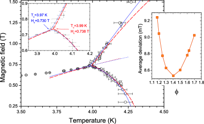
Figure 17: (Color online) Scaling in the vicinity of bicritical point. Blue solid and red dashed lines are fits (8,9,10) with $\phi=1.4$ and $\phi=1.175$ correspondingly, dotted lines are extension of (8) to the $T>T_{c}$ region. Left insert: magnified part of main plot. Right insert: fit deviation (see text) versus critical exponent $\phi$.

The observed dependence of the phase diagram in the bicritical point range on the field orientation is natural, because bicritical point is very sensitive to field misalignmentKing and Rohrer (1979). On the contrary, away from the region around $H_{c}$, the phase boundaries for $\psi=0^{\circ}$ and $\psi=12^{\circ}$ coincide within error bars.

VI Conclusions

In the present work we have studied AFMR spectra and magnetization curves of HSLAFM Cu(pz)₂(ClO₄)₂. These measurements reveal the presence of biaxial anisotropy in Cu(pz)₂(ClO₄)₂, instead of easy-plane formulation used earlier. From the ESR experiments we have derived two energy gaps $\Delta_{z}\simeq 35$ and $\Delta_{y}\simeq 11$ GHz. The weak in-plane anisotropy is responsible for the spin-flop phase transition at $\mu_{0}H_{c}\simeq 0.4$ T in $\mathbf{H}\parallel x$ direction. The AFMR spectra also show, that weak in-plane anisotropy is changing its sign at the spin-flop transition. This anisotropy reversal, occuring in a manner of switching, may be also observed as a phase transition at changing the orientation of the magnetic field within the $bc$ plane, at the critical angle 10^∘ with respect to the easy axis direction. The conjecture that this anomaly might be of magnetoelastic origin may, by simplified treatment, explain the anisotropy reversal at the spin flop, but is not consistent with the step-like angular dependence of ESR field or frequency. It is also not consistent with the observed relation between the energy gap $\Delta_{y}$ and spin-flop field $H_{c}$. The nature of the abrupt reversal of the weak anisotropy remains unclear.

The hypothesis which is probably worth to analyze theoretically is a possible change of the direction and magnitude of zero point spin fluctuations at the spin flop. A change of the contribution of fluctuations to the energy of the anisotropy may also change the effective anisotropy of the ordered spin component.

The field-dependence of the temperature of the minimum on $M(T)$ curves for three principal orientations are found to be in agreement with the results of numerical simulation of HSLAFM Cuccoli et al. (2003). The increase of $T_{N}$ in external field has been found for all orientations in agreement with previous measurements. Scaling exponent $\phi=1.4\pm 0.2$ of phase boundaries near the bicritical point is intermediate between 2D and 3D models.

Accounting for the observed weak anisotropy might be significant for correct estimation of other weak interactions, e.g. next-nearest neighbor and interlayer exchange from experimental dataSiahatgar et al. (2011). Similar anisotropy can be present in another HSLAFM’s of Cu-pz family (namely, Cu(pz)₂(BF₄)₂ and [Cu(pz)₂(NO₃)](PF₆)), as according to Xiao’s magnetization dataXiao et al. (2009) there are signatures of spin-flop transitions as well.

We note that for deuterated Cu(pz)₂(ClO₄)₂ the difference between $b$ and $c$, resulting in the weak anisotropy, is larger than for a regular sample with hydrogen, so it would be of interest to test if the in-plane anisotropy is the same in a deuterated sample. Other possible future experiments include NMR and neutron scattering with field along $x$ to probe the magnetic structure as well as search for anomaly in magnetic field dependencies of low-temperature elastic properties (magnetostriction, ultrasound propagation etc).

VII Acknowledgments

The authors would like to thank O. S. Volkova and A. N. Vasiliev (Moscow State University), and A. Zheludev (ETH Zürich) for the opportunity of using their experimental facilities and assistance with it. Also special thanks to V. N. Glazkov, L. E. Svistov, S. S. Sosin, V. I. Marchenko, M. E. Zhitomirsky and W. E. A. Lorenz for fruitful and stimulating discussions. This work was supported by RFBR Grant No 12-02-00557.

Appendix A AFMR frequencies of a biaxial antiferromagnet

A theory for AFMR in a two-sublattice antiferromagnet with biaxial anisotropy has been developed in 1950’sNagamiya et al. (1955). For both orientations of the magnetic field along hard- and middle-axis ($z$ and $y$), in the ground state we have the antiferromagnetic order parameter $\mathbf{l}\parallel x$, and this orientation of $\mathbf{l}$ is independent of external field magnitude.

Magnetic resonance frequencies for $\mathbf{H}\parallel z$ are

$$\nu_{zz}=\sqrt{(\frac{g_{z}\mu_{B}}{2\pi\hbar}\mu_{0}H)^{2}+\Delta_{z}^{2}},$$ (12)

$$\nu_{zy}=\Delta_{y};$$ (13)

and for $\mathbf{H}\parallel y$ we have

$$\nu_{yy}=\sqrt{(\frac{g_{y}\mu_{B}}{2\pi\hbar}\mu_{0}H)^{2}+\Delta_{y}^{2}},$$ (14)

$$\nu_{yz}=\Delta_{z}.$$ (15)

At the orientation of the magnetic field along the easy axis the case is more complicated, as the ground state is field-dependent. There is a spin-flop transition with an abrupt change from $\mathbf{l}\parallel x$ to $\mathbf{l}\parallel y$. The critical field of this transition is

$$\mu_{0}H_{c}=2\pi\frac{\hbar\Delta_{y}}{g_{x}\mu_{B}}$$ (16)

This transition is accompanied by a jump in magnetization. The ESR frequencies below and above $H_{c}$ are the following:

For $H<H_{c}$:

$$\nu_{1,2}=\sqrt{(\frac{g_{x}\mu_{B}}{2\pi\hbar}\mu_{0}H)^{2}+\frac{\Delta_{y}^{2}+\Delta_{z}^{2}}{2}\mp\sqrt{2(\frac{g_{x}\mu_{B}}{2\pi\hbar}\mu_{0}H)^{2}(\Delta_{y}^{2}+\Delta_{z}^{2})+(\frac{\Delta_{y}^{2}-\Delta_{z}^{2}}{2})^{2}}}\\$$ (17)

For $H>H_{c}$

$$\nu_{4} =\sqrt{(\frac{g_{x}\mu_{B}}{2\pi\hbar}\mu_{0}H)^{2}-\Delta_{y}^{2}}$$ (18)

$$\nu_{5} =\sqrt{\Delta_{z}^{2}-\Delta_{y}^{2}}$$ (19)

The resonant mode $\nu_{3}$ with the vertical $\nu_{3}(H)$ dependence corresponds to spin-flop transition, as the system is allowed to absorb energy in a band of frequencies in the critical point. Modes $\nu_{1}$ and $\nu_{4}$ are softened at the critical field $H_{c}$. For the intermediate field orientations we calculated the frequencies of spin resonance numerically within the same formalism.

Appendix B Magnetoelastic correction

For description of ESR modes at $T\rightarrow 0$ we use macroscopic exchange symmetry formalismAndreev and Marchenko (1980). This formalism, in particular, reproduces the results of a mean-field theory of a two-sublattice antiferromagnet with biaxial anisotropyNagamiya et al. (1955). In the framework of the exchange approach the spin structure is considered to be collinear, and the anisotropy of a relativistic origin, and magnetization,induced by the external field, are taken as perturbations. Though being applicable only in fields $H\ll H_{sat}$, this formalism is model-independent and allows easy introduction of additional anisotropy terms. As the saturation field in Cu(pz)₂(ClO₄)₂ constitutes almost 50 T, restriction on the field magnitude is not an issue for the exchange symmetry formalism applicability. Our calculations are based on the following Lagrange function per mole of the compound (in CGS system):

$$\mathcal{L}=\frac{\chi_{\perp}}{2\gamma^{2}}\left(\dot{\mathbf{l}}+{\gamma}[\mathbf{H}\times\mathbf{l}]\right)^{2}-U_{a}.$$ (20)

Here $\gamma=\dfrac{g\mu_{B}}{\hbar}$ is the gyromagnetic ratio, unit vector $\mathbf{l}$ with the orientation, given by angles $\varphi$ and $\theta$ shown on Fig.4, is the order parameter, $\mathbf{H}$ is magnetic field; $\chi_{\perp}$ is the magnetic susceptibility in the direction, perpendicular to $\mathbf{l}$. Equation (20) also implies $\chi_{\parallel}=0$ at zero temperature. Term $U_{a}=\eta l_{y}^{2}+\zeta l_{z}^{2}$ is the anisotropy energy. We assume positive constants $\eta$ and $\zeta$, $\eta<\zeta$. Hence $\mathbf{l}\parallel x$ minimizes anisotropy energy.

The ground state and magnetic resonance frequencies may be calculated using this Lagrange function, as described in Ref.Andreev and Marchenko, 1980. The ground state and the spectrum are identical to that of Ref. Nagamiya et al., 1955, described above. The anisotropy constants may be expressed via energy gaps: $\eta=\chi_{\perp}(2\pi\Delta^{2}_{y})/2\gamma^{2}$ and $\zeta=\chi_{\perp}(2\pi\Delta^{2})_{z}/2\gamma^{2}$, where $\Delta_{z}>\Delta_{y}$ are the energy gaps, which one actually observes in the ESR experiment. With this substitution, Lagrange function (20) is

$$\begin{split}\mathcal{L}=\frac{\chi_{\perp}}{\gamma^{2}}\left(\frac{1}{2}\left(\dot{\mathbf{l}}+{\gamma}[\mathbf{H}\times\mathbf{l}]\right)^{2}-{}\right.\phantom{abcdefghijk}&\\ -\left.\frac{(2\pi\Delta_{z})^{2}}{2}l_{z}^{2}-\frac{(2\pi\Delta_{y})^{2}}{2}l_{y}^{2}\right)&,\end{split}$$ (21)

and corresponding potential energy in non-zero magnetic field is

$$\begin{split}\mathcal{E}=\frac{\chi_{\perp}}{\gamma^{2}}\left(-\frac{\gamma^{2}}{2}[\mathbf{H}\times\mathbf{l}]^{2}+{}\right.\phantom{abcdefghijklmnop}&\\ +\left.\frac{(2\pi\Delta_{z})^{2}}{2}l_{z}^{2}+\frac{(2\pi\Delta_{y})^{2}}{2}l_{y}^{2}\right)&,\end{split}$$ (22)

Figure 18: (Color online) Spectra of model (23) for various values of quartic term. Field is directed along $x$. Arrows mark frequencies at which angular dependencies for $B=\chi_{\perp}\left(\dfrac{2\pi\hbar\Delta_{y}}{g_{x}\mu_{B}}\right)^{2}$ are shown in the insertion; dashed lines are the expectation for paramagnetic resonance.

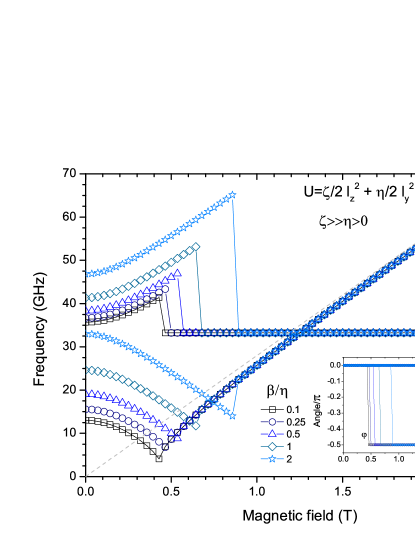
Figure 19: (Color online) Spectra of the model with a quartic term $-\beta l_{x}^{4}$, ${\bf H}\parallel x$. Dashed line is paramagnetic resonance.

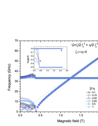
Figure 20: (Color online) Spectra of the model with a quartic term $\beta l_{x}^{4}$, ${\bf H}\parallel x$. Dashed line is paramagnetic resonance.

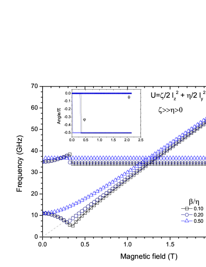
Figure 21: (Color online) Spectra of the model with a quartic term $-\beta l_{y}^{4}$, ${\bf H}\parallel x$. Dashed line is paramagnetic resonance.

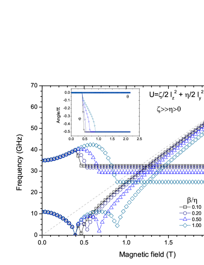
Figure 22: (Color online) Spectra of the model with a quartic term $\beta l_{y}^{4}$, ${\bf H}\parallel x$. Dashed line is paramagnetic resonance.

Monoclinic symmetry allows for another second-order term, $l_{y}l_{z}$. Such a term results in a tilt of hard and middle anisotropy axes, leaving easy axis undisturbed. In our experimental data, related to $xz$ plane rotation of the magnetic field (Fig. 7), we do not notice any significant tilt of middle axis from $c$ direction, and, therefore, we do not take $l_{y}l_{z}$ term into account.

We have to note, that anisotropic term $\eta l_{y}^{2}$ originates from a weak orthorhombic distortion of a square lattice. Due to this distortion, the lattice constants $b$ and $c$ differ in a relative sense for about of ($\sim 10^{-4}$). Hence, this term should be small in comparison with, e.g. $\zeta l_{z}^{2}$, and can be comparable with the contributions of higher order in components of $\mathbf{l}$. There is a term $B(l_{x}l_{y})^{2}$ among the fourth-order terms, allowed by symmetry for Cu(pz)₂(ClO₄)₂. This term couples the components $l_{x},l_{y}$ and could result in the ’anisotropy reversal’ as a result of $\mathbf{l}$ reorientation. Indeed, considering a modified Lagrange function

$$\begin{split}\mathcal{L}=\frac{\chi_{\perp}}{\gamma^{2}}&\left(\frac{1}{2}\left(\dot{\mathbf{l}}+{\gamma}[\mathbf{H}\times\mathbf{l}]\right)^{2}-{}\right.\\ -&\left.\frac{(2\pi\Delta_{z})^{2}}{2}l_{z}^{2}-\frac{(2\pi\Delta_{y})^{2}}{2}l_{y}^{2}\right)+B(l_{x}l_{y})^{2},\end{split}$$ (23)

we obtain approximate frequencies, corresponding to in-plane fluctuations of $\mathbf{l}$, for ground states before and after reorientation:

$$\widetilde{\nu}(l\parallel x)=\sqrt{\Delta_{y}^{2}+\dfrac{2B}{\chi_{\perp}}(\dfrac{g_{x}\mu_{B}}{2\pi\hbar})^{2}-(\dfrac{g_{x}\mu_{B}}{2\pi\hbar}H)^{2}}$$

and

$$\widetilde{\nu}(l\parallel y)=\sqrt{-\Delta_{y}^{2}+\dfrac{2B}{\chi_{\perp}}(\dfrac{g_{x}\mu_{B}}{2\pi\hbar})^{2}+(\dfrac{g_{x}\mu_{B}}{2\pi\hbar}H)^{2}}.$$

The field-independent constants under the square root signs in this relations may be treated by use of model (B2) and relations (A6,A7) as anisotropy constant for in-plane anisotropy (note that these constants should be taken with the opposite signs). Thus, if $B>0$ is large enough, the in-plane anisotropy effectively changes its sign. Significant value of $B$ might be provided by a magnetoelastic interaction. There are 13 elastic terms of the form of $u_{ik}u_{mn}$ and 20 magnetoelastic terms of the form of $u_{ik}l_{m}l_{n}$ allowed by symmetry for Cu(pz)₂(ClO₄)₂ [Lines, 1979]. From these terms we take for the magnetoelastic contribution to potential energy (22) the following terms:

$$E_{me}\propto u_{xy}l_{x}l_{y},$$ (24)

and

$$E_{ee}\propto\frac{u_{xy}^{2}}{2}.$$ (25)

These terms couple $l_{x}$ and $l_{y}$. Here $u_{ik}$ are components of the strain tensor.

Minimization of energy, including described above magnetoelastic correction (24,25), with respect to strain variable $u_{xy}$ will result in the magnetoelastic correction in the form of $Bl_{x}^{2}l_{y}^{2}$.

We numerically calculate ground state and spectrum of the model (23). For our numerical work we choose parameters $\Delta_{z}=37$ and $\Delta_{y}=15$ GHz, and follow the perturbations, introduced by quartic term $Bl_{x}^{2}l_{y}^{2}$. At Fig. 18 numerically calculated spectra for field along $x$ and different values of $B$ (namely, $\dfrac{2B}{\chi_{\perp}}\left(\dfrac{g_{x}\mu_{B}}{2\pi\hbar\Delta_{y}}\right)^{2}=0,0.1,0.5,1,1.5,2$) are present. Indeed, we can choose the value of $B$, which is large enough to push mode $\nu_{4}$ above paramagnetic resonance, as it is clearly seen on Fig. 18. But there remains a crucial difference between the properties of model (23) and experimental data, because the angular dependence is not described. We found from ESR experiment that angular dependence of resonance line shows a step when switching from $\nu_{a}$ to $\nu_{4}$, the anomalous mode $\nu_{a}$ exists in a narrow angle range near the $x$-axis, and outside of this range all the data is perfectly described by a simple biaxial model. In contrast, the model with strong $B$ term (23) shows smooth angular dependence (see insert on Fig. 18), which differs significantly from both simple biaxial model (21) and experimental data (as on Fig. 5). Furthermore, as it is seen from Fig. 18, enhancement of $B$ term also increases a lower zero-field gap, while critical field of spin-flop transition is still determined by $\Delta^{2}_{y}$ alone, as $l_{x}^{2}l_{y}^{2}$ combination gives the same contribution to energies of both $\mathbf{l}\parallel x$ and $\mathbf{l}\parallel y$ phases. Therefore, the magnetoelastic approach (23) predicts the transposition of the antiferromagnetic resonance frequency above the value of the paramagnetic resonance frequency, which is one of the manifestations of the reversal of the in-plane anisotropy. Nevertheless, at the same time, the angular dependence of the resonance field and relation between the gap and critical field do not correspond to the experiment even qualitatively.

Other related quartic terms also could not describe the observed anomaly. We have analyzed in the same way the influence of anisotropic terms $\pm\beta l_{x}^{4}$ and $\pm\beta l_{y}^{4}$. The results of the calculation of the ground states (equilibrium values of $\varphi,\theta$) and frequency-field dependencies are given in Figs. 19, 20, 21, 22. One can see, that it is impossible to find a value of $\beta$ which would correspond to the observed pulling of the frequency above the paramagnetic resonance frequency for $H>H_{c}$ along with the softening of the mode at $H<H_{c}$, and with the valid relation $\gamma H_{c}=\Delta_{y}$.

References

- Manousakis (1991) E. Manousakis, Rev. Mod. Phys., 63, 1 (1991).
- White and Chernyshev (2007) S. R. White and A. L. Chernyshev, Phys. Rev. Lett., 99, 127004 (2007).
- Woodward et al. (2007) F. M. Woodward, P. J. Gibson, G. B. Jameson, C. P. Landee, M. M. Turnbull, and R. D. Willett, Inorg. Chem., 49, 4256 (2007).
- Yasuda et al. (2005) C. Yasuda, S. Todo, K. Hukushima, F. Alet, M. Keller, M. Troyer, and H. Takayama, Phys. Rev. Lett., 94, 217201 (2005).
- Lancaster et al. (2007) T. Lancaster, S. J. Blundell, M. L. Brooks, P. J. Baker, F. L. Pratt, J. L. Manson, M. M. Conner, F. Xiao, C. P. Landee, F. A. Chaves, S. Soriano, M. A. Novak, T. P. Papageorgiou, A. D. Bianchi, T. Herrmannsdörfer, J. Wosnitza, and J. A. Schlueter, Phys. Rev. B, 75, 094421 (2007).
- Tsyrulin et al. (2010) N. Tsyrulin, F. Xiao, A. Schneidewind, P. Link, H. M. Rønnow, J. Gavilano, C. P. Landee, M. M. Turnbull, and M. Kenzelmann, Phys. Rev. B, 102, 134409 (2010a).
- Tsyrulin et al. (2010) N. Tsyrulin, T. Pardini, R. R. P. Singh, F. Xiao, P. Link, A. Schneidewind, A. Hiess, C. P. Landee, M. M. Turnbull, and M. Kenzelmann, Phys. Rev. Lett., 102, 197201 (2010b).
- Cuccoli et al. (2003) A. Cuccoli, T. Roscilde, R. Vaia, and P. Verrucchi, Phys. Rev. Lett., 90, 167205 (2003a).
- Poole (1983) C. Poole, Electron Spin Resonance: A Comprehensive Treatise on Experimental Techniques, Dover books on physics (Dover Publications, 1983) ISBN 9780486694443.
- Nagamiya et al. (1955) T. Nagamiya, K. Yosida, and R. Kubo, Advances in Physics, 4, 1 (1955).
- Fisher (1962) M. E. Fisher, Philosophical Magazine, 7, 1731 (1962).
- Xiao et al. (2009) F. Xiao, F. M. Woodward, C. P. Landee, M. M. Turnbull, C. Mielke, N. Harrison, T. Lancaster, S. J. Blundell, P. J. Baker, P. Babkevich, and F. L. Pratt, Phys. Rev. B, 79, 134412 (2009).
- Morosin (1970) B. Morosin, Phys. Rev. B, 1, 236 (1970).
- Weihong et al. (1991) Z. Weihong, J. Oitmaa, and C. J. Hamer, Phys. Rev. B, 43, 8321 (1991).
- Cuccoli et al. (2003) A. Cuccoli, T. Roscilde, R. Vaia, and P. Verrucchi, Phys. Rev. B, 68, 060402 (2003b).
- Cuccoli et al. (2003) A. Cuccoli, T. Roscilde, V. Tognetti, R. Vaia, and P. Verrucchi, Phys. Rev. B, 67, 104414 (2003c).
- Kosterlitz et al. (1976) J. M. Kosterlitz, D. R. Nelson, and M. E. Fisher, Phys. Rev. B, 13, 412 (1976).
- King and Rohrer (1979) A. R. King and H. Rohrer, Phys. Rev. B, 19, 5864 (1979).
- Nelson and Pelcovits (1977) D. R. Nelson and R. A. Pelcovits, Phys. Rev. B, 16, 2191 (1977).
- Kosterlitz and Santos (1978) J. M. Kosterlitz and M. A. Santos, Journal of Physics C: Solid State Physics, 11, 2835 (1978).
- Cowley et al. (1993) R. Cowley, A. Aharony, R. Birgeneau, R. Pelcovits, G. Shirane, and T. Thurston, Zeitschrift fur Physik B Condensed Matter, 93, 5 (1993), ISSN 0722-3277.
- Holtschneider and Selke (2007) M. Holtschneider and W. Selke, Phys. Rev. B, 76, 220405 (2007).
- Siahatgar et al. (2011) M. Siahatgar, B. Schmidt, and P. Thalmeier, Phys. Rev. B, 84, 064431 (2011).
- Andreev and Marchenko (1980) A. F. Andreev and V. I. Marchenko, Sov. Phys. Usp., 23, 21 (1980).
- Lines (1979) M. Lines, Physics Reports, 55, 133 (1979), ISSN 0370-1573.