Conditional spin counting statistics as a probe of Coulomb interaction and spin-resolved bunching

Abstract

Full counting statistics is a powerful tool to characterize the noise and correlations in transport through mesoscopic systems. In this work, we propose the theory of conditional spin counting statistics, i.e., the statistical fluctuations of spin-up (down) current given the observation of the spin-down (up) current. In the context of transport through a single quantum dot, it is demonstrated that a strong Coulomb interaction leads to a conditional spin counting statistics that exhibits a substantial change in comparison to that without Coulomb repulsion. It thus can be served as an effective way to probe the Coulomb interactions in mesoscopic transport systems. In case of spin polarized transport, it is further shown that the conditional spin counting statistics offers a transparent tool to reveal the spin-resolved bunching behavior.

I Introduction

The exploration of full counting statistics (FCS) in mesoscopic systems has vital roles to play in providing penetrating insight into microscopic mechanisms in transport and temporal correlations between charge carriers which are not accessible from the conventional measurements of time-averaged current alone (2003) (Ed.); Blanter (2005); Blanter and Büttiker (2000). Particularly, recent advances in nanotechnology have made it possible to measure electron transport processes that take place at single-electron level Lu et al. (2003); Fujisawa et al. (2004); Bylander et al. (2005); Elzerman et al. (2004); Schleser et al. (2004); Fujisawa et al. (2006); Gustavsson et al. (2006); Sukhorukov et al. (2007); Gustavsson et al. (2009); Choi et al. (2012). All statistical cumulants of the number of transferred particles can now be extracted experimentally.

Theoretical study of FCS based on the scattering approach turns out to be very powerful for characterizing statistics of noninteracting electron transport through various systems, such as normal-superconductor structures Shelankov and Rammer (2003); Levitov and Reznikov (2004); Belzig and Nazarov (2001a, b), chaotic cavities Pilgram et al. (2003); Nagaev et al. (2004); Pilgram et al. (2004); Novaes (2007, 2008), and electron entanglement detection devices Sim and Sukhorukov (2006); Giovannetti et al. (2006, 2007). Yet, with continued miniaturization of the system size, the involving many-particle interactions become increasingly important in mesoscopic transport Peercy (2000); Kouwenhoven et al. (2001). For that purpose, a generalized quantum master equation (QME) approach has been established by Bagrets and Nazarov, with the Coulomb interactions being fully taken into account Bagrets and Nazarov (2003). This approach has been widely employed to analyze the FCS in a variety of structures, for instance, quantum dot (QD) systems Belzig (2005); Kießlich et al. (2006); Groth et al. (2006); Wang et al. (2007); Welack et al. (2008); Urban and König (2009); Xue (2013), molecules Imura et al. (2007); Xue et al. (2010); Weymann et al. (2012); Xue et al. (2011a, b), and nanoelectromechanical resonators Flindt et al. (2005); Novotný et al. (2004); Rodrigues and Armour (2005). Furthermore, the QME approach was recently extended to investigate finite-frequency FCS Emary et al. (2007); Marcos et al. (2011) as well as non-Markovian dynamics Aguado and Brandes (2004); Braggio et al. (2006); Flindt et al. (2008); Jin et al. (2011); Luo et al. (2013).

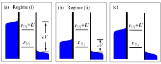
Figure 1: Schematic setup of transport through a single QD in different bias configurations. (a) Regime (i): The bias is large enough to overcome the Coulomb interaction such that the two excitation energies $\epsilon_{\sigma}$ and $\epsilon_{\sigma}+U$ are within the bias window. (b) Regime (ii): A small bias is applied across the QD, and only excitation energy $\epsilon_{\sigma}$ lies in the bias window. Double occupation on the QD is prohibited. (c) The bias voltage is applied in such a way that double occupation on the QD is partially allowed. It offers an interpolation between the regimes (i) and (ii).

For statistically independent tunneling events, the current fluctuations exhibit Poissonian statistics. Normally, the presence of Pauli exclusion principle, which prohibits two fermions of the same spin to be superimposed, leads to the suppression of the current noise below the Poisson value Chen and Ting (1991); Martin and Landauer (1992). On the other hand, Coulomb repulsion acts as another important correlation mechanism that might enhance or inhibit noise, depending on different physical regimes concerned Martin and Büttiker (2000); Blanter and Büttiker (1999); Sukhorukov et al. (2001); Cottet et al. (2004); Kießlich et al. (2007); Urban et al. (2008). Yet, in reality it is quite difficult to distinguish the effects of Coulomb repulsion and the Pauli principle in the charge current noise. It is thus instructive to find a transparent and direct way to characterize the degree of Coulomb correlation in mesoscopic transport. For this purpose, we propose in this work the theory of conditional spin counting statistics: The statistical fluctuations of spin up (down) current given the observation of the spin down (up) current. The inspiration of this theory comes from fact that the Pauli exclusion principle only acts on fermions of the same spin, while electrons with opposite spins are only correlated via the Coulomb repulsion.

First, we consider electron transport through a single QD tunnel-coupled to two normal electrodes. Although the net current is spin unpolarized, the up and down spins are intrinsically correlated to each other via Coulomb repulsion. It is demonstrated that the Coulomb correlation gives rise to conditional spin counting statistics that exhibits a substantial change in comparison to the uncorrelated one. It thus may be utilized as an effective way to characterize the Coulomb correlation in various mesoscopic transport systems.

Second, we investigate conditional spin counting statistics for spin polarized transport by taking into account ferromagnetic electrodes. It is worthwhile to mention that the (unconditional) spin counting statistics has been studied for many years Lorenzo and Nazarov (2004); Schmidt et al. (2007); Sauret and Feinberg (2004); Luo et al. (2008). It was shown that spin current noise can be utilized to detect spin unit of quasiparticles Wang et al. (2004), to sensitively probe spin decoherence in a spin battery Dong et al. (2005), to reveal the discrete nature of the photon states for a quantum dot coupled to a cavity field Djuric and Search (2006). In comparison with the unconditional spin counting statistics, we will show the conditional one may serve as a transparent and sensitive tool to investigate spin-resolved bunching behavior.

The rest of the paper is organized as follows. In Section II, we describe the single QD system under different bias configurations, corresponding to different effectiveness of the Coulomb correlations. We discuss in Section III the charge FCS, which will be compared with the conditional spin counting statistics in sensing the Coulomb repulsion. Section IV is devoted to the theory of conditional spin counting statistics. Its application to the single QD system is demonstrated in Section V, with focus on its effectiveness in characterizing Coulomb correlation and spin-resolved bunching behavior. It is then followed by the conclusion in Section VI.

II The Model

We consider electron transport through a single QD with Coulomb interaction, as schematically shown in Fig. 1. The entire system is described by the Hamiltonian $H=H_{{\rm B}}+H_{\rm QD}+H^{\prime}$, with

$$H_{{\rm B}}=\sum_{\alpha={\rm L},{\rm R}}\sum_{k\sigma}\epsilon_{\alpha k\sigma}c_{\alpha k\sigma}^{\dagger}c_{\alpha k\sigma},$$ (1a)

$$H_{\rm QD}=\sum_{\sigma}\varepsilon_{\sigma}d_{\sigma}^{\dagger}d_{\sigma}+Un_{\uparrow}n_{\downarrow},$$ (1b)

$$H^{\prime}=\sum_{\alpha={\rm L},{\rm R}}\sum_{k\sigma}(t_{\alpha k\sigma}c_{\alpha k\sigma}^{\dagger}d_{\sigma}+{\rm h.c.}).$$ (1c)

Here $H_{\rm B}$ models the noninteracting electrons in the left ($\alpha$=L) and right ($\alpha$=R) electrodes, with $c_{\alpha k\sigma}^{\dagger}$ ($c_{\alpha k\sigma}$) the electron creation (annihilation) operator in the corresponding electrode. The electron distributions in the electrodes are governed by the electrochemical potentials $\mu_{\rm L}$ and $\mu_{\rm R}$, which define the voltage $eV=\mu_{\rm L}-\mu_{\rm R}$. $H_{\rm QD}$ describes the QD with one spin-degenerate energy level $\varepsilon_{\sigma}$ and the Coulomb interaction $U$ on the dot, where $n_{\sigma}=d_{\sigma}^{\dagger}d_{\sigma}$ is the occupation operator, with $d_{\sigma}^{\dagger}$ ($d_{\sigma}$) the electron annihilation (creation) operator in the QD. Electron tunneling between electrodes and QD is depicted by $H^{\prime}$. The tunneling rate for a spin-$\sigma$ electron is characterized by the intrinsic tunneling width $\Gamma_{\alpha\sigma}(\omega)=2\pi\sum_{k}|t_{\alpha k\sigma}|^{2}\delta(\epsilon_{\alpha k\sigma}-\omega)$. Hereafter we consider normal electrodes, i.e. $\Gamma_{\alpha\uparrow}=\Gamma_{\alpha\downarrow}$, and assume flat bands in the electrodes, which yields energy-independent couplings $\Gamma_{\alpha\sigma}$. The total tunnel-coupling strength thus is given by $\Gamma_{\alpha}=\Gamma_{\alpha\uparrow}+\Gamma_{\alpha\downarrow}$. Throughout this work, we set $\hbar=1$ for the Planck constant, unless stated otherwise.

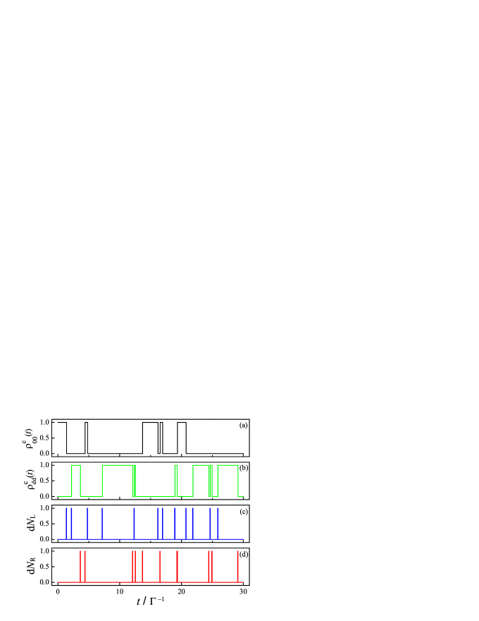
Figure 2: Set of real-time density matrix elements $\rho^{\rm c}_{00}(t)$ and $\rho^{\rm c}_{\rm dd}(t)$ for the regime (i), corresponding to the instantaneous states of empty and doubly occupied QD, respectively. The jumps in $\rho^{\rm c}_{00}(t)$ and $\rho^{\rm c}_{\rm dd}(t)$ are directly related to random electron process of tunneling into/out of the QD, represented by the stochastic variables d$N_{{\rm L}/{\rm R}}$. The unidirectional flow of electrons allows one to count electrons transporting through the system, leading thus to the spectrum of FCS. We assume symmetric tunnel-couplings, i.e. $\Gamma_{\rm L}=\Gamma_{\rm R}$, and $\Gamma=\Gamma_{\rm L}+\Gamma_{\rm R}$.

By specifying which excitation energies lie within the energy window defined by the Fermi levels $\mu_{\rm L}$ and $\mu_{\rm R}$, the following bias configurations will be considered. Regime (i): The bias is large enough to overcome the Coulomb interaction and thus the excitation energy levels $\epsilon_{\sigma}$ and $\epsilon_{\sigma}+U$ are within the bias window defined by chemical potentials $\mu_{\rm L}$ and $\mu_{\rm R}$, as schematically shown in Fig. 1(a). The involving states include $|0\rangle$-empty QD, $|\sigma\rangle$-single occupation by a spin-$\sigma$ electron, and $|{\rm d}\rangle$-double occupation. Regime (ii): Only the single level $\varepsilon_{\sigma}$ is within the bias window, as shown in Fig. 1(b). The charge transport is maximally correlated. The states available are $|0\rangle$-empty QD and $|\sigma\rangle$-singly occupied by a spin-$\sigma$ electron. By appropriately applying the gate and bias voltages, the system can be tuned to the situation between the regimes (i) and (ii) as shown in Fig. 1(c). It allows us to analyze the effect of finite Coulomb correlation on the conditional spin counting statistics between the uncorrelated and maximally correlation cases. Our analysis is based on a second-order Born-Markov quantum master equation for $\Gamma\ll k_{\rm B}T$, where the sequential tunneling processes play the dominant role Gurvitz and Prager (1996); Gurvitz and Mozyrsky (2008). Higher order tunneling events, such as cotunneling, Kondo effect are thus suppressed. An approach of this type has been widely used in the literature for studying bias voltage dependent transport characteristics in various nanostructures Haug and Jauho (1996), such as single Belzig (2005); Thielmann et al. (2003); Kießlich et al. (2003) or double QD Wunsch et al. (2005), where typical step-like transport features were revealed. In spite of the simple model considered here, we will show that it is adequate to address the essence of the conditional spin counting statistics and its effectiveness of characterizing the Coulomb correlation and investigate spin-resolved bunching characteristics.

III Charge Full Counting Statistics

In the single electron tunneling regime, an extra electron can inject into the QD from the left electrode, dwell in the QD for a certain amount of time before it escapes to the right electrode. This stochastic process produces intriguing signatures of the electronic conductor. To study the fluctuations involved in transport, we will utilize a Monte Carlo approach to simulate the individual electron tunneling events. We first introduce two stochastic variables d$N_{{\rm L}\sigma}(t)$ and d$N_{{\rm R}\sigma}(t)$ (with values either 0 or 1) to represent, respectively, the numbers of spin-$\sigma$ electron injected into the QD from the left electrode and that escaped to the right electrode from the QD, during the small time interval d$t$. One then arrives at the following conditional QME Goan et al. (2001)

$${\rm d}\rho^{\rm c} \!\!=\!\! -{\rm i}{\cal L}\rho^{\rm c}(t){\rm d}t-\sum_{\sigma=\uparrow,\downarrow}\{\Gamma_{{\rm L}\sigma}{\cal A}[d^{\dagger}_{\sigma}]+\Gamma_{{\rm R}\sigma}{\cal A}[d_{\sigma}]$$ (2)

$$-{\cal P}_{{\rm L}\sigma}(t)-{\cal P}_{{\rm R}\sigma}(t)\}\rho^{\rm c}(t){\rm d}t$$

$$+\sum_{\sigma=\uparrow,\downarrow}{\rm d}N_{{\rm L}\sigma}\left[\frac{\Gamma_{{\rm L}\sigma}{\cal J}[d^{\dagger}_{\sigma}]}{{\cal P}_{{\rm L}\sigma}(t)}-1\right]\rho^{{\rm c}}(t)$$

$$+\sum_{\sigma=\uparrow,\downarrow}{\rm d}N_{{\rm R}\sigma}\left[\frac{\Gamma_{{\rm R}\sigma}{\cal J}[d_{\sigma}]}{{\cal P}_{{\rm R}\sigma}(t)}-1\right]\rho^{{\rm c}}(t),$$

where the involving superoperators are defined as ${\cal L}\rho^{\rm c}\equiv[H_{\rm QD},\rho^{\rm c}]$, ${\cal J}[X]\rho^{{\rm c}}\equiv X\rho^{{\rm c}}X^{\dagger}$ and ${\cal A}[X]\rho^{{\rm c}}\equiv\frac{1}{2}(X^{\dagger}X\rho^{{\rm c}}+\rho^{{\rm c}}X^{\dagger}X)$. The superscript “c” attached to the reduced density matrix denotes that the quantum state is conditioned on the measurement results. For single electron tunneling events (point process), the two classical random variables satisfy

$$E[{\rm d}N_{{\rm L}\sigma}(t)]={\cal P}_{{\rm L}\sigma}(t){\rm d}t={\rm Tr}\{{\cal J}[\sqrt{\Gamma_{{\rm L}\sigma}}d_{\sigma}^{\dagger}]\rho^{{\rm c}}\}{\rm d}t,$$ (3a)

$$E[{\rm d}N_{{\rm R}\sigma}(t)]={\cal P}_{{\rm R}\sigma}(t){\rm d}t={\rm Tr}\{{\cal J}[\sqrt{\Gamma_{{\rm R}\sigma}}d_{\sigma}]\rho^{{\rm c}}\}{\rm d}t,$$ (3b)

where $E[X]$ stands for an ensemble average of a classical stochastic process $X$. Eq. (2) implies that electron tunneling events condition the future evolution of the reduced density matrix, while Eq. (3) indicates the instantaneous reduced density matrix conditions the detected electron tunneling events. Within this approach, one thus is capable of propagating the conditioned reduced density matrix ($\rho^{\rm c}$) and measurement record (d$N_{\alpha\sigma}$) self-consistently.

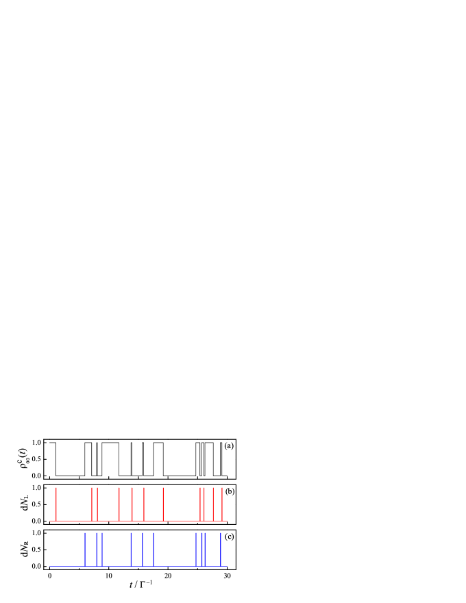
Figure 3: Set of real-time quantum state $\rho^{\rm c}_{00}$ and corresponding detection records of tunneling into/out of the QD (d$N_{{\rm L}/{\rm R}}$) for the regime (ii), where double occupation on the QD is prohibited. The other parameters are the same as those in Fig. 2.

For the regime (i), the excitation energies $\epsilon_{\sigma}$ and $\epsilon_{\sigma}+U$ are within the bias window defined by the chemical potentials of the left and right electrodes. The QD can be empty, singly or doubly occupied. The instantaneous states of an empty [$\rho^{{\rm c}}_{00}(t)$] and doubly occupied [$\rho^{{\rm c}}_{\rm dd}(t)$] QD are displayed in Fig. 2(a) and (b), respectively. A “$1\rightarrow 0$” transition in $\rho^{{\rm c}}_{00}$ or the “$0\rightarrow 1$” one in $\rho^{{\rm c}}_{\rm dd}(t)$ indicates that an electron tunneled into QD from the left electrode (d$N_{{\rm L}}=1$), as shown in Fig. 2(c). The opposite transitions “$0\rightarrow 1$” in $\rho^{{\rm c}}_{00}$ and “$1\rightarrow 0$” in $\rho^{{\rm c}}_{\rm dd}(t)$ imply tunneling events out of QD to the right electrode (d$N_{{\rm R}}=1$) [cf. Fig. 2(d)]. Here d$N_{\alpha}=\sum_{\sigma}$d$N_{\alpha\sigma}$ is the detected charge tunneling events, regardless of the spin orientations. The randomness in nonequilibrium charge transport are intimately related to the intriguing signatures of the electronic conductor, known as the full counting statistics. It can be described under the framework of counting field-dressed approach, in which electron tunnelings between reduced quantum system and the electrodes are taken into account by introducing a corresponding counting field $\chi$. This results in a $\chi$-resolved quantum master equation, which in the Born-Markov limit can be formally written as Levitov et al. (1996); Aguado and Brandes (2004); Braggio et al. (2006); Flindt et al. (2008); Bagrets and Nazarov (2003) $\frac{\partial}{\partial t}{\rho}(\chi,t)={\cal L}_{\chi}\rho(\chi,t)$. All the cumulants of FCS can be obtained by taking derivatives of the cumulant generating function (CGF), which is determined from the lowest eigenvalue of ${\cal L}_{\chi}$. For instance, the CGF in the regime (i) is given by Bagrets and Nazarov (2003)

$${\cal F}_{1}(\chi)=-t_{\rm c}\{\Gamma_{\rm L}\!+\!\Gamma_{\rm R}-\sqrt{(\Gamma_{\rm L}\!-\!\Gamma_{\rm R})^{2}+4\Gamma_{\rm L}\Gamma_{\rm R}e^{-{\rm i}\chi}}\},$$ (4)

where the counting time $t_{\rm c}$ satisfies $t_{\rm c}\gg\Gamma_{{\rm L}/{\rm R}}^{-1}$.

In the regime (ii), the excitation energy $\epsilon_{\sigma}+U$ stays well above the the Fermi level. Double occupation on the QD is prohibited, thus electrons can only transport through the single-level $\epsilon_{\sigma}$. The available Fock states are reduced to $|0\rangle$-empty QD and $|\sigma\rangle$-single occupation by a spin-$\sigma$ electron. The real-time state $\rho_{00}^{{\rm c}}(t)$ is sufficient to characterize electron tunneling events as shown in Fig. 3. Whenever $\rho_{00}^{{\rm c}}(t)$ jumps from 1 to 0, it reveals an electron has tunneled into the QD from the left electrode (d$N_{{\rm L}}=1$), while the ‘0$\rightarrow$1’ jump implies the tunneling out event to the right electrode (d$N_{{\rm R}}=1$), as displayed in Fig. 3(b) and (c), respectively. By counting the single electron tunneling events, one obtains the CGF in the regime (ii)

$${\cal F}_{2}(\chi)\!=\!-\frac{t_{\rm c}}{2}\{2\Gamma_{\rm L}\!+\!\Gamma_{\rm R}\!-\!\sqrt{(2\Gamma_{\rm L}\!-\!\Gamma_{\rm R})^{2}\!+\!8\Gamma_{\rm L}\Gamma_{\rm R}e^{-{\rm i}\chi}}\}.$$ (5)

Apparently, the result for the regime (ii) [Eq. (5)] is qualitatively similar to that of the regime (i) [Eq. (4)], except for an effective doubling of the tunneling rate $\Gamma_{\rm L}$. This simple example shows that the charge FCS might not be the best possible probe of Coulomb interactions. On the contrary, we will show later that the intriguing behavior of conditional spin counting statistics can be utilized to reveal the Coulomb correlation between the up and down spins unambiguously.

IV Conditional Spin Counting Statistics

Now we introduce the theory of conditional spin counting statistics: The statistical fluctuations of the spin-$\uparrow$ ($\downarrow$) current, given the observation of a given spin-$\downarrow$ ($\uparrow$) current. It might be calculated from the conditional distribution function $P(I_{\uparrow}|I_{\downarrow})$ [$P(I_{\downarrow}|I_{\uparrow})$], the probability of observing spin-$\uparrow$ ($\downarrow$) current conditioned on an observation of a spin-$\downarrow$ ($\uparrow$) one. To obtain the mixed generating functions of conditional spin counting statistics, we introduce spin-resolved counting fields $\chi_{\uparrow}$ and $\chi_{\downarrow}$, which are used to characterize, respectively, jumps of up and down spins through a specific junction. The corresponding ($\chi_{\uparrow}$,$\chi_{\downarrow}$)-resolved master equation can be formally written as $\frac{\partial}{\partial t}\rho(\chi_{\uparrow},\chi_{\downarrow},t)=M(\chi_{\uparrow},\chi_{\downarrow})\rho(\chi_{\uparrow},\chi_{\downarrow},t)$. In the steady state ($t_{\rm c}\gg\Gamma_{{\rm L}/{\rm R}}^{-1}$), the joint generating function ${\cal F}(\chi_{\uparrow},\chi_{\downarrow}$) is determined from the minimal eigenvalue of $M$ according to

$${\cal F}(\chi_{\uparrow},\chi_{\downarrow})=-\lambda_{\rm min}(\chi_{\uparrow},\chi_{\downarrow})t_{\rm c},$$ (6)

where $\lambda_{\rm min}$ satisfies $\lambda_{\rm min}(\chi_{\uparrow}\rightarrow 0,\chi_{\downarrow}\rightarrow 0)\rightarrow 0$.

From the definition of the joint generating function, the joint probability distribution of transmitted spins can be extracted by Fourier transforming on both variables,

$$P(N_{\uparrow},N_{\downarrow},t_{\rm c})=\!\int_{0}^{2\pi}\!\frac{{\rm d}\chi_{\uparrow}{\rm d}\chi_{\downarrow}}{(2\pi)^{2}}e^{-\lambda_{\rm min}t_{\rm c}-{\rm i}(N_{\uparrow}\chi_{\uparrow}+N_{\downarrow}\chi_{\downarrow})},$$ (7)

where $N_{\uparrow}=I_{\uparrow}t_{\rm c}$ and $N_{\downarrow}=I_{\downarrow}t_{\rm c}$. In the stationary limit, it is justified to evaluate the integral in the saddle point approximation Bagrets and Nazarov (2003); Pilgram et al. (2003); Utsumi et al. (2006); Utsumi (2007). The dominant term contributing to the joint distribution is then given by

$$P(I_{\uparrow},I_{\downarrow},t_{\rm c})=-t_{\rm c}{\rm min}_{\chi_{\uparrow},\chi_{\downarrow}}\{\lambda_{\rm min}+{\rm i}I_{\uparrow}\chi_{\uparrow}+{\rm i}I_{\downarrow}\chi_{\downarrow}\}.$$ (8)

The mixed generating functions of conditional spin counting statistics may be calculated by only Fourier transforming on one of the above variables in Eq. (8). For instance, integrating over the $\chi_{\uparrow}$ variable yields ${\cal F}(\chi_{\uparrow},I_{\downarrow})$. Due to the Bayes theorem, which relates the joint distribution and conditional distribution functions $P(I_{\uparrow},I_{\downarrow})=P(I_{\uparrow}|I_{\downarrow})P(I_{\downarrow})=P(I_{\downarrow}|I_{\uparrow})P(I_{\uparrow})$, the mixed generating function then is given by ${\cal F}(\chi_{\uparrow}|I_{\downarrow})={\cal F}(\chi_{\uparrow},I_{\downarrow})-{\cal F}(0,I_{\downarrow})$. The statistical fluctuations of spin $\uparrow$ current given the observation of a spin $\downarrow$ current can be obtained from ${\cal F}(\chi_{\uparrow}|I_{\downarrow})$ by performing derivatives with respect to the counting field $\chi_{\uparrow}$

$$\langle I_{\uparrow}^{k}\rangle_{I_{\downarrow}}=-\frac{(-{\rm i}\partial_{\chi_{\uparrow}})^{k}}{t_{\rm c}}{\cal F}(\chi_{\uparrow}|I_{\downarrow})|_{\chi_{\uparrow}\rightarrow 0}.$$ (9)

Analogously, the conditional spin counting statistics of spin $\downarrow$ current can be obtained from ${\cal F}(\chi_{\downarrow}|I_{\uparrow})$.

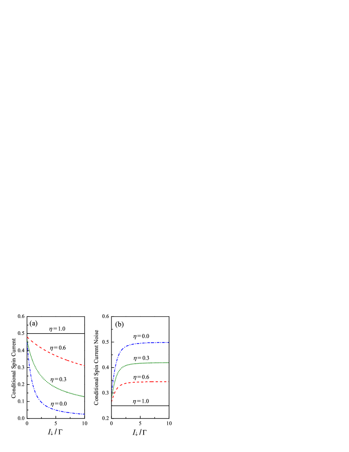
Figure 4: (a) Conditional spin-$\uparrow$ current and (b) its noise as functions of given spin-$\downarrow$ currents for different values of $\eta$. The tunnel-couplings are symmetric, i.e. $\Gamma_{\rm L}=\Gamma_{\rm R}=1.0$. The currents are measured in unit of $\Gamma=\Gamma_{\rm L}+\Gamma_{\rm R}$.

V Results and Discussion

First let us focus on the regime (i), as schematically shown in Fig. 1(a). The involving states are $|0\rangle$-empty dot, $|\!\!\uparrow/\downarrow\rangle$-occupation by a spin-$\uparrow\!/\!\downarrow$ electron, and $|{\rm d}\rangle$-doubly occupied. The ($\chi_{\uparrow},\chi_{\downarrow}$)-resolved quantum master equation reads $\frac{\partial}{\partial t}\rho(\chi_{\uparrow},\chi_{\downarrow})=M_{1}(\chi_{\uparrow},\chi_{\downarrow})\rho(\chi_{\uparrow},\chi_{\downarrow})$, where $M_{1}$ is a 4$\times$4 matrix

$$M_{1}=\left(\begin{array}[]{cccc}-2\Gamma_{\rm L}&e^{{\rm i}\chi_{\uparrow}}\Gamma_{\rm R}&e^{{\rm i}\chi_{\downarrow}}\Gamma_{\rm R}&0\\ \Gamma_{\rm L}&-\Gamma_{\rm L}-\Gamma_{\rm R}&0&e^{{\rm i}\chi_{\downarrow}}\Gamma_{\rm R}\\ \Gamma_{\rm L}&0&-\Gamma_{\rm L}-\Gamma_{\rm R}&e^{{\rm i}\chi_{\uparrow}}\Gamma_{\rm R}\\ 0&\Gamma_{\rm L}&\Gamma_{\rm L}&-2\Gamma_{\rm R}\end{array}\right).$$ (14)

The minimal eigenvalue of $M_{1}$ is then determined, which leads to the joint distribution $P_{1}(I_{\uparrow},I_{\downarrow},t_{\rm c})$ of spin $\uparrow$ and $\downarrow$ currents

$$\frac{\log P_{1}}{t_{\rm c}}\!=\!-(\Gamma_{\rm L}+\Gamma_{\rm R})+\!\sum_{\sigma=\uparrow,\downarrow}\!\left\{\frac{\Omega_{\sigma}}{2}\!-\!I_{\sigma}\log\left(\frac{\Omega_{\sigma}I_{\sigma}}{\Gamma_{\rm L}\Gamma_{\rm R}}\right)\right\},$$ (15)

with $\Omega_{\sigma}=2I_{\sigma}+\sqrt{4I_{\sigma}^{2}+(\Gamma_{\rm L}-\Gamma_{\rm R})^{2}}$. Apparently, the joint probability factorizes $P_{1}(I_{\uparrow},I_{\downarrow})=P(I_{\uparrow})P(I_{\downarrow})$, which implies that spin-$\uparrow$ and spin-$\downarrow$ currents are uncorrelated. The resultant mixed generating function for conditional spin counting statistics then reads

$${\cal F}_{1}(\chi_{\uparrow}|I_{\downarrow})\!=\!-\frac{t_{\rm c}}{2}\{\Gamma_{\rm L}+\Gamma_{\rm R}-\sqrt{(\Gamma_{\rm L}\!-\!\Gamma_{\rm R})^{2}\!+\!4\Gamma_{\rm L}\Gamma_{\rm R}e^{-{\rm i}\chi_{\uparrow}}}\},$$ (16)

analogous to the charge counting statistics in the regime (i) in Eq. (4), except for an overall factor of $\frac{1}{2}$. The spin transport through the QD independently, thus each spin component contributes 50% of the total current. The cumulants of conditional spin counting statistics are thus the same as those of unconditional ones. For instance, the first and second mixed cumulants are given, respectively, by

$$\langle I_{\uparrow}\rangle_{I_{\downarrow}}=\frac{\Gamma_{\rm L}\Gamma_{\rm R}}{\Gamma_{\rm L}+\Gamma_{\rm R}},$$ (17)

$$\frac{\langle I^{2}_{\uparrow}\rangle_{I_{\downarrow}}}{2e\langle I_{\uparrow}\rangle_{I_{\downarrow}}}=1-\frac{2\Gamma_{\rm L}\Gamma_{\rm R}}{(\Gamma_{\rm L}+\Gamma_{\rm R})^{2}}.$$ (18)

Thus, in this case the system can be mapped onto that transport through a single level without Coulomb interaction.

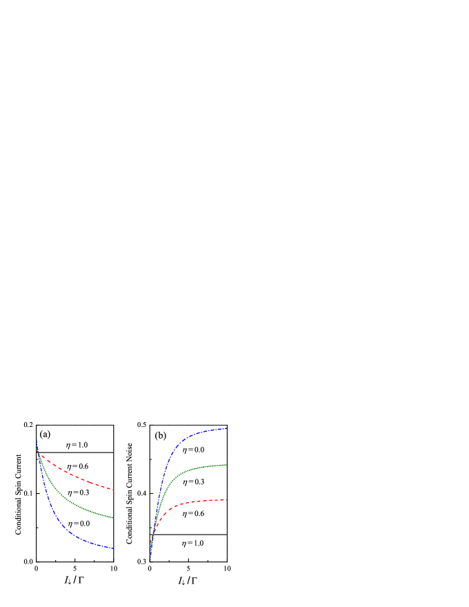
Figure 5: Conditional spin-$\uparrow$ current and its noise versus $I_{\downarrow}$ for asymmetric tunnel-couplings $\Gamma_{\rm R}=4\Gamma_{\rm L}$. The other parameters are the same as those in Fig. 4.

Let us now consider the conditional spin counting statistics in the regime (ii) as shown in Fig. 1(b), where at most one electron can be occupied and thus up and down spins are maximally correlated. The involving states are reduced to $|0\rangle$-empty dot, $|\!\uparrow$/$\downarrow\rangle$-occupied by a spin $\uparrow$/$\downarrow$ electron. The spin-resolved quantum master equation reads $\frac{\partial}{\partial t}\rho(\chi_{\uparrow},\chi_{\downarrow})=M_{2}(\chi_{\uparrow},\chi_{\downarrow})\rho(\chi_{\uparrow},\chi_{\downarrow})$, where $M_{2}$ is the 3$\times$3 matrix, given by

$$M_{2}=\left(\begin{array}[]{ccc}-2\Gamma_{\rm L}&e^{{\rm i}\chi_{\uparrow}}\Gamma_{\rm R}&e^{{\rm i}\chi_{\downarrow}}\Gamma_{\rm R}\\ \Gamma_{\rm L}&-\Gamma_{\rm R}&0\\ \Gamma_{\rm L}&0&-\Gamma_{\rm R}\end{array}\right).$$ (22)

The minimal eigenvalue can be readily evaluated, which results in the joint probability for the spin currents

$$\frac{\log P_{2}}{t_{\rm c}}=\frac{1}{2}(\Lambda-2\Gamma_{\rm L}-\Gamma_{\rm R})-\sum_{\sigma}I_{\sigma}\log\left(\frac{\Lambda I_{\sigma}}{\Gamma_{\rm L}\Gamma_{\rm R}}\right),$$ (23)

where $\Lambda=2(I_{\uparrow}+I_{\downarrow})+\sqrt{4(I_{\uparrow}+I_{\downarrow})^{2}+(2\Gamma_{\rm L}-\Gamma_{\rm R})^{2}}$. The term inside the logarithm shows unambiguously that the spin-$\uparrow$ and spin-$\downarrow$ currents are correlated. Further integrating over the $\chi_{\uparrow}$ variable gives rise to the mixed generating function

$${\cal F}_{2}(\chi_{\uparrow}|I_{\downarrow})\!=\!\frac{t_{\rm c}}{2}\left\{G(\chi_{\uparrow})\!-\!G(0)\!-\!2I_{\downarrow}\log\!\left[\frac{2I_{\downarrow}\!+\!G(\chi_{\uparrow})}{2I_{\downarrow}+G(0)}\right]\right\},$$ (24)

with $G({\chi_{\uparrow}})=\sqrt{4I_{\downarrow}^{2}+4e^{\chi_{\uparrow}}\Gamma_{\rm L}\Gamma_{\rm R}+(2\Gamma_{\rm L}-\Gamma_{\rm R})^{2}}$. The conditional spin counting statistics can be calculated via taking derivatives with respective to $\chi_{\uparrow}$. For instance, the first mixed cumulant yields the conditional spin current

$$\langle I_{\uparrow}\rangle_{I_{\downarrow}}=\frac{\Gamma_{\rm L}\Gamma_{\rm R}}{2I_{\downarrow}+G(0)},$$ (25a)

and the second mixed cumulant corresponds to the conditional shot noise of spin $$\uparrow$$ current

$$\frac{\langle I^{2}_{\uparrow}\rangle_{I_{\downarrow}}}{e\langle I_{\uparrow}\rangle_{I_{\downarrow}}}=1-\frac{2\Gamma_{\rm L}\Gamma_{\rm R}}{[2I_{\downarrow}+G(0)]G(0)},$$ (25b)

where $G(0)=\sqrt{4I_{\downarrow}^{2}+4\Gamma_{\rm L}^{2}+\Gamma_{\rm R}^{2}}$. Both conditional current and noise show radical changes in comparison with the uncorrelated ones [see Eq. (17) for the regime (i)].

It is also instructive to compare the conditional spin counting statistics with the unconditional one. By utilizing Eq. (22), the first two cumulants of the unconditional spin counting statistics are given, respectively, by

$$\langle I_{\uparrow}\rangle_{\rm un}=\frac{\Gamma_{\rm L}\Gamma_{\rm R}}{2\Gamma_{\rm L}+\Gamma_{\rm R}},$$ (26)

$$\frac{\langle I^{2}_{\uparrow}\rangle_{\rm un}}{e\langle I_{\uparrow}\rangle_{\rm un}}=1-\frac{2\Gamma_{\rm L}\Gamma_{\rm R}}{(2\Gamma_{\rm L}+\Gamma_{\rm R})^{2}}.$$ (27)

Except for an effective doubling of “$\Gamma_{\rm L}$”, these two cumulants are found to be qualitatively analogous to the results in regime (i). We will shown, on the contrary, that the conditional spin counting statistics is much more sensitive to the Coulomb repulsion. In case of spin polarized transport, it will be revealed that the conditional spin counting statistics can be served as transparent tool to investigate spin-resolved bunching behavior in mesoscopic transport.

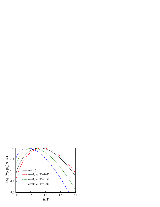
Figure 6: Conditional spin current statistics versus $I_{\uparrow}$ for uncorrelated ($\eta=1.0$) and maximally correlated ($\eta=0.0$) transport. Other parameters are the same as those in Fig. 5.

We are now in a position to investigate the conditional spin counting statistics between the regimes (i) and (ii), as shown in Fig. 1(c). It thus offers an interpolation between the uncorrelated and the maximally correlated regimes. In experiments, it can be realized via tuning appropriately the gate and bias voltages, shifting thus the excitation energies ($\epsilon_{\sigma}$ and $\epsilon_{\sigma}+U$) relative to the Fermi levels of the left and right electrodes in such a way that double occupation on the QD is partially allowed Ono et al. (2002). The corresponding rate matrix is then given by

$$M_{3}=\left(\begin{array}[]{cccc}-2\Gamma_{\rm L}&e^{{\rm i}\chi_{\uparrow}}\Gamma_{\rm R}&e^{{\rm i}\chi_{\downarrow}}\Gamma_{\rm R}&0\\ \Gamma_{\rm L}&-\eta\Gamma_{\rm L}-\Gamma_{\rm R}&0&(1-\eta)\Gamma_{\rm L}+e^{{\rm i}\chi_{\downarrow}}\Gamma_{\rm R}\\ \Gamma_{\rm L}&0&-\eta\Gamma_{\rm L}-\Gamma_{\rm R}&(1-\eta)\Gamma_{\rm L}+e^{{\rm i}\chi_{\uparrow}}\Gamma_{\rm R}\\ 0&\eta\Gamma_{\rm L}&\eta\Gamma_{\rm L}&-2(1-\eta)\Gamma_{\rm L}-2\Gamma_{\rm R}\end{array}\right),$$ (32)

where $\eta=\{1+e^{\beta(\epsilon_{\sigma}+U-\mu_{\rm L})}\}^{-1}$ represents the Fermi function. If the excitation energy $\epsilon_{\sigma}+U$ is well below $\mu_{\rm L}$, $\eta$ approaches 1 and $M_{3}$ reduces to $M_{1}$, corresponding to uncorrelated transport. In the opposite limit of $\epsilon_{\sigma}+U\gg\mu_{\rm L}$, $\eta$ goes to zero and $M_{3}\rightarrow M_{2}$, leading thus to the regime of maximal correlation. The rate matrix $M_{3}$ thus allows us to investigate an interpolation between the two extreme cases.

The numerical results of conditional spin current and its shot noise are displayed in Fig. 4(a) and (b), respectively, for symmetric tunnel-couplings ($\Gamma_{\rm L}=\Gamma_{\rm R}$). The conditioned spin-$\uparrow$ current decreases monotonically with the spin-$\downarrow$ current, and tends to 0 as $I_{\downarrow}\rightarrow\infty$. The conditional shot noise of spin-$\uparrow$ current, however, increases with $I_{\downarrow}$. For a given $I_{\downarrow}$, the spin-$\uparrow$ current grows with rising $\eta$, approaching the maximum at $\eta=1.0$ corresponding to uncorrelated transport. Yet, the conditional noise decreases as $\eta$ rises, and reaches the minimum at $\eta=1.0$. Unambiguously, in the regime $I_{\downarrow}/\Gamma\gg 1$, both conditional current and noise are very sensitive to $\eta$, thus showing them as sensitive tools to probe the Coulomb correlation.

Fig. 5 shows the first two conditional cumulants for asymmetric tunnel-couplings ($\Gamma_{\rm R}=4\Gamma_{\rm L}$). The results are qualitatively similar to those in Fig. 4, except for the regime of small $I_{\downarrow}$ ($I_{\downarrow}/\Gamma\lesssim 1$), where finite Coulomb correlation leads to a spin-$\uparrow$ current exceeding the uncorrelated one ($\eta=1.0$). This can be explained in terms of the conditional spin current statistics $P(I_{\uparrow}|I_{\downarrow})$, as shown in Fig. 6. Consider the situation of maximal correlation ($\eta=0$). For a given small spin-$\downarrow$ current (see the dashed curve for $I_{\downarrow}/\Gamma=0.05$), the average of the conditional probability is slightly larger than that of uncorrelated transport ($\eta=1.0$), resulting thus in the unique behavior in the regime of small $I_{\downarrow}$. With increasing $I_{\downarrow}$, the average of the distribution decreases [see, for instance, the dotted curve for $I_{\downarrow}/\Gamma=1.5$]. Eventually, it results in suppressed conditional current in comparison with the uncorrelated transport, as displayed in Fig. 5. Interestingly, it is found that in the limit of maximal correlation ($\eta=0$), the conditional noise reaches the maximum $\frac{1}{2}$ as $I_{\downarrow}\rightarrow\infty$, regardless of the ratio between the two tunneling rates $\Gamma_{\rm L}/\Gamma_{\rm R}$ [cf. Eq. (25b)]. It actually reflects the rare tunneling events of up spins through the QD system given an extremely large spin-$\downarrow$ current.

So far, our analysis has been focused only on the situation where the transport is spin unpolarized. Now we account for finite polarization due to ferromagnetic electrodes, which give rise to polarization-dependent tunneling rates. Consider, for instance, the parallel magnetic configuration when the majority of electrons in both electrodes point in the same direction. The rates of tunneling through the left and right electrodes are

$$\Gamma_{{\rm L}\uparrow/{\rm L}\downarrow}=(1\pm p)\Gamma_{\rm L}\quad{\rm and}\quad\Gamma_{{\rm R}\uparrow/{\rm R}\downarrow}=(1\pm p)\Gamma_{\rm R},$$ (33)

respectively, where we have assumed the same polarization $p$ $(0\leq p\leq 1)$ in the left and right electrodes. In the limit of maximum correlation ($\eta=0$), the corresponding rate matrix is reduced to

$$M_{4}=\left(\begin{array}[]{ccc}-2\Gamma_{\rm L}&e^{{\rm i}\chi_{\uparrow}}(1+p)\Gamma_{\rm R}&e^{{\rm i}\chi_{\downarrow}}(1-p)\Gamma_{\rm R}\\ (1+p)\Gamma_{\rm L}&-(1+p)\Gamma_{\rm R}&0\\ (1-p)\Gamma_{\rm L}&0&-(1-p)\Gamma_{\rm R}\end{array}\right).$$ (37)

The unconditional spin $\uparrow$ current and its noise are given by

$$\langle I_{\uparrow}\rangle_{\rm un} \!\!\!=\!\!\! (1+p)\frac{\Gamma_{\rm L}\Gamma_{\rm R}}{2\Gamma_{\rm L}+\Gamma_{\rm R}},$$ (38a)

$$\frac{\langle I^{2}_{\uparrow}\rangle_{\rm un}}{e\langle I_{\uparrow}\rangle_{\rm un}} \!\!\!=\!\!\! 1-\frac{2\Gamma_{\rm L}\Gamma_{\rm R}}{(2\Gamma_{\rm L}+\Gamma_{\rm R})^{2}}+\frac{4p\Gamma_{\rm L}^{2}}{(1-p)(2\Gamma_{\rm L}+\Gamma_{\rm R})^{2}}.$$ (38b)

In the limit $p\rightarrow 0$, one recovers the results in Eq. (26). Both current and noise increase with the polarization $p$. In particular, the unconditional spin current noise may increase dramatically, and even diverge as $p\rightarrow 1$.

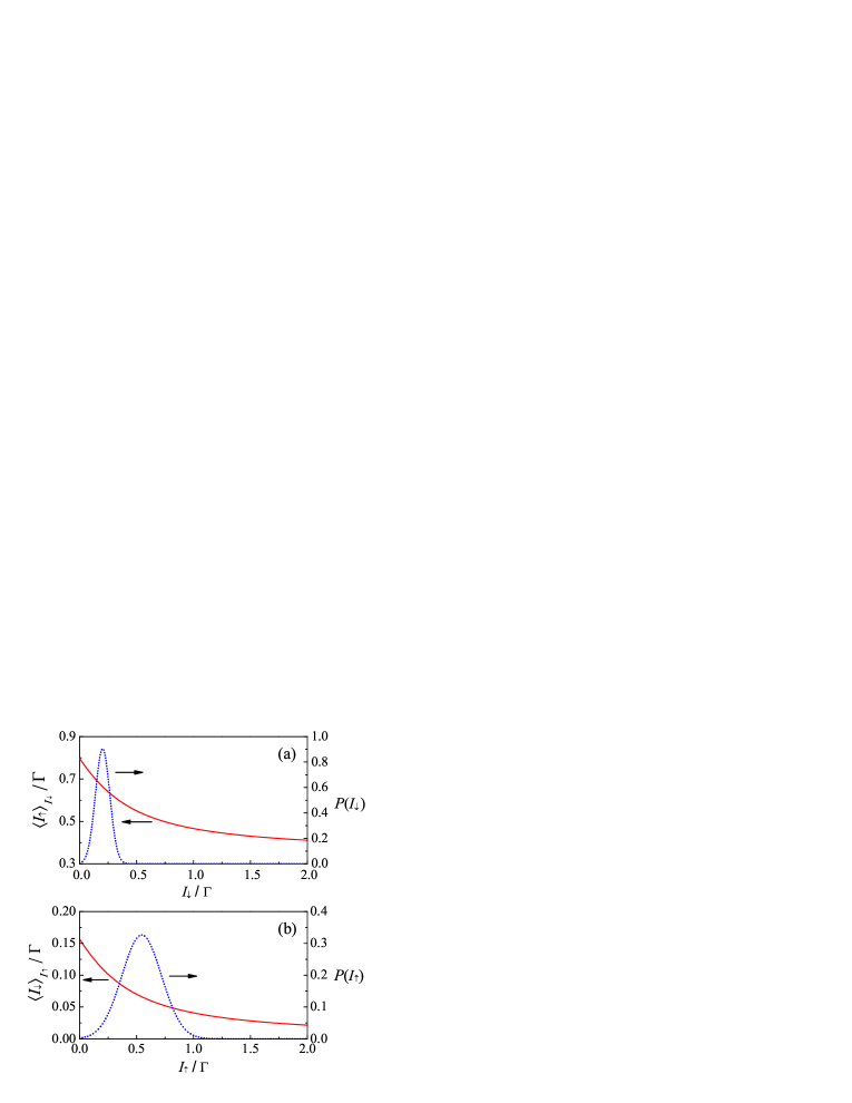
Figure 7: (a) Conditional spin $\uparrow$ current, (b) spin $\downarrow$ current, and their related probabilities [$P(I_{\downarrow})$ and $P(I_{\uparrow})$] for polarization $p$=0.5 and symmetric tunnel-couplings $\Gamma_{\rm L}=\Gamma_{\rm R}=\Gamma/2$.

To further elucidate the underlying mechanism, we employ the conditional spin counting statistics. It is inferred from the Bayes theorem and Eq. (9) that

$$\langle I_{\uparrow}\rangle_{\rm un}=\int_{0}^{\infty}{\rm d}I_{\downarrow}P(I_{\downarrow})\langle I_{\uparrow}\rangle_{I_{\downarrow}},$$ (39)

where $P(I_{\downarrow})$ is the probability distribution of the spin $\downarrow$ current that can be obtained from Eq. (37). It allows us to analyze contribution to the unconditional spin current under various circumstances. Fig. 7 shows the numerical results of the conditional spin current and related probability for polarization $p=0.5$ and symmetric tunnel-couplings. It is illustrated unambiguously in Fig. 7(a) that the major contribution to the unconditional spin $\uparrow$ current ($\langle I_{\uparrow}\rangle_{\rm un}$) comes from a large conditional spin $\uparrow$ current ($\langle I_{\uparrow}\rangle_{I_{\downarrow}}\sim 0.6\Gamma$) at small spin $\downarrow$ current in the narrow window defined by the probability $P(I_{\downarrow})$, i.e. $I_{\downarrow}\sim(0.2\pm 0.1)\Gamma$. It reveals the bunching of up spins due to a dynamical blockade of a small spin $\downarrow$ current, which eventually results in the prominent super-Poissonian noise as $p\rightarrow 1$. On the contrary, for $\langle I_{\downarrow}\rangle_{\rm un}$ the main contribution is from the low unconditional spin $\downarrow$ current within a wide range of spin $\uparrow$ current $I_{\downarrow}\sim(0.5\pm 0.3)\Gamma$, as shown in Fig. 7(b). The noise of spin $\downarrow$ current is thus suppressed below the Poisson value, as we have checked. Despite this simple QD system, our analysis demonstrated that the conditional spin counting statistics is a sensitive and useful tool to investigate spin-resolved bunching behavior and its connection to the noise characteristics.

Finally, let us propose a scheme to measure the conditional spin counting statistics. Instead of using the normal electrodes, we consider a four-terminal device: A single QD tunnel-coupled to four fully spin polarized ferromagnetic electrodes Sauret and Feinberg (2004); Sánchez et al. (2003). The two left (right) electrodes are kept at the same chemical potential $\mu_{\rm L}$ ($\mu_{\rm R}$) but with opposite spin polarizations. The junction parameters are set the same for the two left electrodes, and likewise for the two on the right, such that the net current transport through the device is not spin polarized and the proposed four-terminal setup can be mapped onto the model we have analyzed. The great advantage of this scheme is that it is possible to measure separately the up or down spin current in each of the four electrodes, even though the net current is not spin polarized. Thus, it eventually enables us to measure the conditional spin counting statistics. We expect these predictions would be tested in quantum transport experiments in the near future.

VI Conclusion

In summary, we have proposed the theory of conditional spin counting statistics: The statistical fluctuations of one spin current component, given the observation of another spin current component. In the context of transport through a single quantum dot, we demonstrated that the presence of a Coulomb correlation leads to conditional spin counting statistics that exhibits a substantial change in comparison to the uncorrelated one. It thus can be served as an effective way to characterize the Coulomb correlation in mesoscopic transport systems. We further show that in the spin polarized transport, the conditional spin counting statistics offers a transparent and sensitive tool to understand the spin-resolved bunching behavior and its connection to the noise characteristics in mesoscopic transport.Emary et al. (2012).

- (1) Y. V. N. (Ed.), Quantum Noise in Mesoscopic Physics (Kluwer Academic Publishers, Dordrecht, 2003).
- Blanter (2005) Y. M. Blanter, arXiv:cond-mat/0511478 (2005).
- Blanter and Büttiker (2000) Y. M. Blanter and M. Büttiker, Phys. Rep. 336, 1 (2000).
- Lu et al. (2003) W. Lu, Z. Ji, L. Pfeiffer, K. W. West, and A. J. Rimberg, Nature 423, 422 (2003).
- Fujisawa et al. (2004) T. Fujisawa, T. Hayashi, Y. Hirayama, H. D. Cheong, and Y. H. Jeong, Appl. Phys. Lett. 84, 2343 (2004).
- Bylander et al. (2005) J. Bylander, T. Duty, and P. Delsing, Nature 434, 361 (2005).
- Elzerman et al. (2004) J. M. Elzerman, R. Hanson, L. H. W. van Beveren, B. Witkamp, L. M. K. Vandersypen, and L. P. Kouwenhoven, Nature 430, 431 (2004).
- Schleser et al. (2004) R. Schleser, E. Ruh, T. Ihn, K. Ensslin, D. C. Driscoll, and A. C. Gossard, Appl. Phys. Lett. 85, 2005 (2004).
- Fujisawa et al. (2006) T. Fujisawa, T. Hayashi, R. Tomita, and Y. Hirayama, Science 312, 1634 (2006).
- Gustavsson et al. (2006) S. Gustavsson, R. Leturcq, B. Simovic, R. Schleser, T. Ihn, P. Studerus, K. Ensslin, D. C. Driscoll, and A. C. Gossard, Phys. Rev. Lett. 96, 076605 (2006).
- Sukhorukov et al. (2007) E. V. Sukhorukov, A. N. Jordan, S. Gustavsson, R. Leturcq, T. Ihn, and K. Ensslin, Nature Phys. 3, 243 (2007).
- Gustavsson et al. (2009) S. Gustavsson, R. Leturcq, M. Studer, I. Shorubalko, T. Ihn, K. Ensslin, D. Driscoll, and A. Gossard, Surf. Sci. Rep. 64, 191 (2009).
- Choi et al. (2012) T. Choi, T. Ihn, S. Schön, and K. Ensslin, arXiv:1202.4273 (2012).
- Shelankov and Rammer (2003) A. Shelankov and J. Rammer, Europhys. Lett. 63, 485 (2003).
- Levitov and Reznikov (2004) L. S. Levitov and M. Reznikov, Phys. Rev. B 70, 115305 (2004).
- Belzig and Nazarov (2001a) W. Belzig and Y. V. Nazarov, Phys. Rev. Lett. 87, 067006 (2001a).
- Belzig and Nazarov (2001b) W. Belzig and Y. V. Nazarov, Phys. Rev. Lett. 87, 197006 (2001b).
- Pilgram et al. (2003) S. Pilgram, A. N. Jordan, E. V. Sukhorukov, and M. Büttiker, Phys. Rev. Lett. 90, 206801 (2003).
- Nagaev et al. (2004) K. E. Nagaev, S. Pilgram, and M. Büttiker, Phys. Rev. Lett. 92, 176804 (2004).
- Pilgram et al. (2004) S. Pilgram, K. E. Nagaev, and M. Büttiker, Phys. Rev. B 70, 045304 (2004).
- Novaes (2007) M. Novaes, Phys. Rev. B 75, 073304 (2007).
- Novaes (2008) M. Novaes, Phys. Rev. B 78, 035337 (2008).
- Sim and Sukhorukov (2006) H.-S. Sim and E. V. Sukhorukov, Phys. Rev. Lett. 96, 020407 (2006).
- Giovannetti et al. (2006) V. Giovannetti, D. Frustaglia, F. Taddei, and R. Fazio, Phys. Rev. B 74, 115315 (2006).
- Giovannetti et al. (2007) V. Giovannetti, D. Frustaglia, F. Taddei, and R. Fazio, Phys. Rev. B 75, 241305 (2007).
- Peercy (2000) P. S. Peercy, Nature 406, 1023 (2000).
- Kouwenhoven et al. (2001) L. P. Kouwenhoven, D. G. Austing, and S. Tarucha, Rep. Prog. Phys. 64, 701 (2001).
- Bagrets and Nazarov (2003) D. A. Bagrets and Y. V. Nazarov, Phys. Rev. B 67, 085316 (2003).
- Belzig (2005) W. Belzig, Phys. Rev. B 71, 161301 (2005).
- Kießlich et al. (2006) G. Kießlich, P. Samuelsson, A. Wacker, and E. Schöll, Phys. Rev. B 73, 033312 (2006).
- Groth et al. (2006) C. W. Groth, B. Michaelis, and C. W. J. Beenakker, Phys. Rev. B 74, 125315 (2006).
- Wang et al. (2007) S.-K. Wang, H. Jiao, F. Li, X.-Q. Li, and Y. J. Yan, Phys. Rev. B 76, 125416 (2007).
- Welack et al. (2008) S. Welack, M. Esposito, U. Harbola, and S. Mukamel, Phys. Rev. B 77, 195315 (2008).
- Urban and König (2009) D. Urban and J. König, Phys. Rev. B 79, 165319 (2009).
- Xue (2013) H.-B. Xue, Ann. Phys. 339, 208 (2013).
- Imura et al. (2007) K.-I. Imura, Y. Utsumi, and T. Martin, Phys. Rev. B 75, 205341 (2007).
- Xue et al. (2010) H.-B. Xue, Y.-H. Nie, Z.-J. Li, and J.-Q. Liang, J. Appl. Phys. 108, 033707 (2010).
- Weymann et al. (2012) I. Weymann, J. Barnaś, and S. Krompiewski, Phys. Rev. B 85, 205306 (2012).
- Xue et al. (2011a) H.-B. Xue, Y.-H. Nie, Z.-J. Li, and J.-Q. Liang, Phys. Lett. A 375, 716 (2011a).
- Xue et al. (2011b) H.-B. Xue, Y.-H. Nie, Z.-J. Li, and J.-Q. Liang, J. Appl. Phys. 109, 083706 (2011b).
- Flindt et al. (2005) C. Flindt, T. Novotný, and A.-P. Jauho, Physica E 29, 411 (2005).
- Novotný et al. (2004) T. Novotný, A. Donarini, C. Flindt, and A.-P. Jauho, Phys. Rev. Lett. 92, 248302 (2004).
- Rodrigues and Armour (2005) D. A. Rodrigues and A. D. Armour, Phys. Rev. B 72, 085324 (2005).
- Emary et al. (2007) C. Emary, D. Marcos, R. Aguado, and T. Brandes, Phys. Rev. B 76, 161404 (2007).
- Marcos et al. (2011) D. Marcos, C. Emary, T. Brandes, and R. Aguado, Phys. Rev. B 83, 125426 (2011).
- Aguado and Brandes (2004) R. Aguado and T. Brandes, Phys. Rev. Lett. 92, 206601 (2004).
- Braggio et al. (2006) A. Braggio, J. König, and R. Fazio, Phys. Rev. Lett. 96, 026805 (2006).
- Flindt et al. (2008) C. Flindt, T. Novotný, A. Braggio, M. Sassetti, and A.-P. Jauho, Phys. Rev. Lett. 100, 150601 (2008).
- Jin et al. (2011) J. Jin, X.-Q. Li, M. Luo, and Y. J. Yan, J. Appl. Phys. 109, 053704 (2011).
- Luo et al. (2013) J. Y. Luo, H. J. Jiao, B. T. Xiong, X.-L. He, and C. R. Wang, J. Appl. Phys. 114, 173703 (2013).
- Chen and Ting (1991) L. Y. Chen and C. S. Ting, Phys. Rev. B 43, 4534 (1991).
- Martin and Landauer (1992) T. Martin and R. Landauer, Phys. Rev. B 45, 1742 (1992).
- Martin and Büttiker (2000) M. A. Martin and M. Büttiker, Phys. Rev. Lett. 84, 3386 (2000).
- Blanter and Büttiker (1999) Y. M. Blanter and M. Büttiker, Phys. Rev. B 59, 10217 (1999).
- Sukhorukov et al. (2001) E. V. Sukhorukov, G. Burkard, and D. Loss, Phys. Rev. B 63, 125315 (2001).
- Cottet et al. (2004) A. Cottet, W. Belzig, and C. Bruder, Phys. Rev. Lett. 92, 206801 (2004).
- Kießlich et al. (2007) G. Kießlich, E. Schöll, T. Brandes, F. Hohls, and R. J. Haug, Phys. Rev. Lett. 99, 206602 (2007).
- Urban et al. (2008) D. Urban, J. König, and R. Fazio, Phys. Rev. B 78, 075318 (2008).
- Lorenzo and Nazarov (2004) A. D. Lorenzo and Y. V. Nazarov, Phys. Rev. Lett. 93, 046601 (2004).
- Schmidt et al. (2007) T. L. Schmidt, A. O. Gogolin, and A. Komnik, Phys. Rev. B 75, 235105 (2007).
- Sauret and Feinberg (2004) O. Sauret and D. Feinberg, Phys. Rev. Lett. 92, 106601 (2004).
- Luo et al. (2008) J. Y. Luo, X.-Q. Li, and Y. J. Yan, J. Phys.: Cond. Matt. 20, 345215 (2008).
- Wang et al. (2004) B. Wang, J. Wang, and H. Guo, Phys. Rev. B 69, 153301 (2004).
- Dong et al. (2005) B. Dong, H. L. Cui, and X. L. Lei, Phys. Rev. Lett. 94, 066601 (2005).
- Djuric and Search (2006) I. Djuric and C. P. Search, Phys. Rev. B 74, 115327 (2006).
- Gurvitz and Prager (1996) S. A. Gurvitz and Y. S. Prager, Phys. Rev. B 53, 15932 (1996).
- Gurvitz and Mozyrsky (2008) S. A. Gurvitz and D. Mozyrsky, Phys. Rev. B 77, 075325 (2008).
- Haug and Jauho (1996) H. Haug and A.-P. Jauho, Quantum Kinetics in Transport and Optics of Semiconductors (Springer-Verlag, Berlin, 1996).
- Thielmann et al. (2003) A. Thielmann, M. H. Hettler, J. König, and G. Schön, Phys. Rev. B 68, 115105 (2003).
- Kießlich et al. (2003) G. Kießlich, A. Wacker, and E. Schöll, Phys. Rev. B 68, 125320 (2003).
- Wunsch et al. (2005) B. Wunsch, M. Braun, J. König, and D. Pfannkuche, Phys. Rev. B 72, 205319 (2005).
- Goan et al. (2001) H. S. Goan, G. J. Milburn, H. M. Wiseman, and H. B. Sun, Phys. Rev. B 63, 125326 (2001).
- Levitov et al. (1996) L. S. Levitov, H. W. Lee, and G. B. Lesovik, J. Math. Phys. 37, 4845 (1996).
- Utsumi et al. (2006) Y. Utsumi, D. S. Golubev, and G. Schön, Phys. Rev. Lett. 96, 086803 (2006).
- Utsumi (2007) Y. Utsumi, Phys. Rev. B 75, 035333 (2007).
- Ono et al. (2002) K. Ono, D. G. Austing, Y. Tokura, and S. Tarucha, Science 297, 1313 (2002).
- Sánchez et al. (2003) D. Sánchez, R. López, P. Samuelsson, and M. Büttiker, Phys. Rev. B 68, 214501 (2003).
- Emary et al. (2012) C. Emary, C. Pöltl, A. Carmele, J. Kabuss, A. Knorr, and T. Brandes, Phys. Rev. B 85, 165417 (2012).