Multivariate varying coefficient model for functional responses

Abstract

Motivated by recent work studying massive imaging data in the neuroimaging literature, we propose multivariate varying coefficient models (MVCM) for modeling the relation between multiple functional responses and a set of covariates. We develop several statistical inference procedures for MVCM and systematically study their theoretical properties. We first establish the weak convergence of the local linear estimate of coefficient functions, as well as its asymptotic bias and variance, and then we derive asymptotic bias and mean integrated squared error of smoothed individual functions and their uniform convergence rate. We establish the uniform convergence rate of the estimated covariance function of the individual functions and its associated eigenvalue and eigenfunctions. We propose a global test for linear hypotheses of varying coefficient functions, and derive its asymptotic distribution under the null hypothesis. We also propose a simultaneous confidence band for each individual effect curve. We conduct Monte Carlo simulation to examine the finite-sample performance of the proposed procedures. We apply MVCM to investigate the development of white matter diffusivities along the genu tract of the corpus callosum in a clinical study of neurodevelopment.

, and

t1Supported by NIH Grants RR025747-01, P01CA142538-01, MH086633, EB005149-01 and AG033387.

t2Supported by NSF Grant DMS-03-48869, NIH Grants P50-DA10075 and R21-DA024260 and NNSF of China 11028103. The content is solely the responsibility of the authors and does not necessarily represent the official views of the NSF or the NIH.

1 Introduction

With modern imaging techniques, massive imaging data can be observed over both time and space Towle1993 , Fass2008 , Niedermeyer2004 , Buzsaki2006 , Friston2009 , Heywood2006 . Such imaging techniques include functional magnetic resonance imaging (fMRI), electroencephalography (EEG), diffusion tensor imaging (DTI), positron emission tomography (PET) and single photon emission-computed tomography (SPECT) among many other imaging techniques. See, for example, a recent review of multiple biomedical imaging techniques and their applications in cancer detection and prevention in Fass Fass2008 . Among them, predominant functional imaging techniques including fMRI and EEG have been widely used in behavioral and cognitive neuroscience to understand functional segregation and integration of different brain regions in a single subject and across different populations Friston2009 , Friston2007 , Huettel2004 . In DTI, multiple diffusion properties are measured along common major white matter fiber tracts across multiple subjects to characterize the structure and orientation of white matter structure in human brain in vivo Basser1994b , Basser1994a , Zhu2007b .

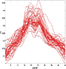
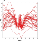
(a)	(b)
(c)	(d)

Figure 1: Representative functional neuroimaging data: (a) and (b) FA and MD along the genu tract of the corpus callosum from 40 randomly selected infants; and (c) and (d) the estimated hemodynamic response functions (HRF) corresponding to two stimulus categories from 14 subjects.

A common feature of many imaging techniques is that massive functional data are observed/calculated at the same design points, such as time for functional images (e.g., PET and fMRI). As an illustration, we present two smoothed functional data as an illustration and a real imaging data in Section 6, that we encounter in neuroimaging studies. First, we plot two diffusion properties, called fractional anisotropy (FA) and mean diffusivity (MD), measured at 45 grid points along the genu tract of the corpus callosum [Figure 1(a) and (b)] from 40 randomly selected infants from a clinical study of neurodevelopment with more than 500 infants. Scientists are particularly interested in delineating the structure of the variability of these functional FA and MD data and their association with a set of covariates of interest, such as age. We will systematically investigate the development of FA and MD along the genu of the corpus callosum tract in Section 6. Second, we consider the BOLD fMRI signal, which is based on hemodynamic responses secondary to neural activity. We plot the estimated hemodynamic response functions (HRF) corresponding to two stimulus categories from 14 randomly selected subjects at a selected voxel of a common template space from a clinical study of Alzheimer’s disease with more than 100 infants. Although the canonical form of the HRF is often used, when applying fMRI in a clinical population with possibly altered hemodynamic responses [Figure 1(c) and (d)], using the subject’s own HRF in fMRI data analysis may be advantageous because HRF variability is greater across subjects than across brain regions within a subject Lindquist2008 , AguirreZarahn1998 . We are particularly interested in delineating the structure of the variability of the HRF and their association with a set of covariates of interest, such as diagnostic group Lindquist2008b .

A varying-coefficient model, which allows its regression coefficients to vary over some predictors of interest, is a powerful statistical tool for addressing these scientific questions. Since it was systematically introduced to statistical literature by Hastie and Tibshirani HastieTibshirani1993 , many varying-coefficient models have been widely studied and developed for longitudinal, time series and functional data MR1742497 , MR1769751 , MR1959093 , MR2425354 , MR2504204 , MR1666699 , Ramsay2005 , MR2087972 , MR1888349 , Zhang2007 , MR2523900 . However, most varying-coefficient models in the existing literature are developed for univariate response. Let ${\mathbf{y}}_{i}(s)=(y_{i1}(s),\ldots,y_{iJ}(s))^{T}$ be a $J$-dimensional functional response vector for subject $i$, $i=1,\ldots,n$, and ${\mathbf{x}}_{i}$ be its associated $p\times 1$ vector of covariates of interest. Moreover, $s$ varies in a compact subset of Euclidean space and denotes the design point, such as time for functional images and voxel for structural and functional images. For notational simplicity, we assume $s\in[0,1]$, but our results can be easily extended to higher dimensions. A multivariate varying coefficient model (MVCM) is defined as

$${y}_{ij}(s)={\mathbf{x}}_{i}^{T}B_{j}(s)+\eta_{ij}(s)+\varepsilon_{ij}(s)\qquad\mbox{for }j=1,\ldots,J,$$ (1)

where $B_{j}(s)=(b_{j1}(s),\ldots,b_{jp}(s))^{T}$ is a $p\times 1$ vector of functions of $s$, $\varepsilon_{ij}(s)$ are measurement errors, and $\eta_{ij}(s)$ characterizes individual curve variations from ${\mathbf{x}}_{i}^{T}B_{j}(s)$. Moreover, $\{\eta_{ij}(s)\dvtx s\in[0,1]\}$ is assumed to be a stochastic process indexed by $s\in[0,1]$ and used to characterize the within-curve dependence. For image data, it is typical that the $J$ functional responses ${\mathbf{y}}_{i}(s)$ are measured at the same location for all subjects and exhibit both the within-curve and between-curve dependence structure. Thus, for ease of notation, it is assumed throughout this paper that ${\mathbf{y}}_{i}(s)$ was measured at the same $M$ location points $s_{1}=0\leq s_{2}\leq\cdots\leq s_{M}=1$ for all $i$.

Most varying coefficient models in the existing literature coincide model (1) with $J=1$ and without the within-curve dependence. Statistical inferences for these varying coefficient models have been relatively well studied. Particularly, Hoover et al. MR1666699 and Wu, Chiang and Hoover WuChiang1998 were among the first to introduce the time-varying coefficient models for analysis of longitudinal data. Recently, Fan and Zhang MR2425354 gave a comprehensive review of various statistical procedures proposed for many varying coefficient models. It is of particular interest in data analysis to construct simultaneous confidence bands (SCB) for any linear combination of $B_{j}$ instead of pointwise confidence intervals and to develop global test statistics for the general hypothesis testing problem on $B_{j}$. For univariate varying coefficient models without the within-curve dependence, Fan and Zhang MR1804172 constructed SCB using the limit theory for the maximum of the normalized deviation of the estimate from its expected value. Faraway Faraway1997 , Chiou, Müller and Wang Chiou2004 , and Cardot Cardot2007 proposed several varying coefficient models and their associated estimators for univariate functional response, but they did not give functional central limit theorem and simultaneous confidence band for their estimators. It has been technically difficult to carry out statistical inferences including simultaneous confidence band and global test statistic on $B_{j}$ in the presence of the within-curve dependence.

There have been several recent attempts to solve this problem in various settings. For time series data, which may be viewed as a case with $n=1$ and $M\rightarrow\infty$, asymptotic SCB for coefficient functions in varying coefficient models can be built by using local kernel regression and a Gaussian approximation result for nonstationary time series ZhouWu2010 . For sparse irregular longitudinal data, Ma, Yang and Carroll MaYang2011 constructed asymptotic SCB for the mean function of the functional regression model by using piecewise constant spline estimation and a strong approximation result. For functional data, Degras Degras2011 constructed asymptotic SCB for the mean function of the functional linear model without considering any covariate, while Zhang and Chen Zhang2007 adopted the method of “smoothing first, then estimation” and propose a global test statistic for testing $B_{j}$, but their results cannot be used for constructing SCB for $B_{j}$. Recently, Cardot et al. Cardot2010 , Cardot and Josserand Cardot2011 built asymptotic SCB for Horvitz–Thompson estimators for the mean function, but their models and estimation methods differ significantly from ours.

In this paper, we propose an estimation procedure for the multivariate varying coefficient model (1) by using local linear regression techniques, and derive a simultaneous confidence band for the regression coefficient functions. We further develop a test for linear hypotheses of coefficient functions. The major aim of this paper is to investigate the theoretical properties of the proposed estimation procedure and test statistics. The theoretical development is challenging, but of great interest for carrying out statistical inferences on $B_{j}$. The major contributions of this paper are summarized as follows. We first establish the weak convergence of the local linear estimator of $B_{j}$, denoted by $\hat{B}_{j}$, by using advanced empirical process methods VaartWellner1996 , Kosorok2008 . We further derive the bias and asymptotic variance of $\hat{B}_{j}$. These results provide insight into how the direct estimation procedure for $B_{j}$ using observations from all subjects outperforms the estimation procedure with the strategy of “smoothing first, then estimation.” After calculating $\hat{B}_{j}$, we reconstruct all individual functions $\eta_{ij}$ and establish their uniform convergence rates. We derive uniform convergence rates of the proposed estimate for the covariance matrix of $\eta_{ij}$ and its associated eigenvalue and eigenvector functions by using related results in Li and Hsing LiHsing2010 . Using the weak convergence of the local linear estimator of $B_{j}$, we further establish the asymptotic distribution of a global test statistic for linear hypotheses of the regression coefficient functions, and construct an asymptotic SCB for each varying coefficient function.

The rest of this paper is organized as follows. In Section 2, we describe MVCM and its estimation procedure. In Section 3, we propose a global test statistic for linear hypotheses of the regression coefficient functions and construct an asymptotic SCB for each coefficient function. In Section 4, we discuss the theoretical properties of estimation and inference procedures. Two sets of simulation studies are presented in Section 5 with the known ground truth to examine the finite sample performance of the global test statistic and SCB for each individual varying coefficient function. In Section 6, we use MVCM to investigate the development of white matter diffusivities along the genu tract of the corpus callosum in a clinical study of neurodevelopment.

2 Estimation procedure

Throughout this paper, we assume that ${\bolds{\varepsilon}}_{i}(s)=(\varepsilon_{i1}(s),\ldots,\varepsilon_{iJ}(s))^{T}$ and ${\bolds{\eta}}_{i}(s)=(\eta_{i1}(s),\ldots,\eta_{iJ}(s))^{T}$ are mutually independent, and ${\bolds{\eta}}_{i}(s)$ and ${\bolds{\varepsilon}}_{i}(s)$ are independent and identical copies of SP$({\mathbf{0}},\Sigma_{\eta})$ and SP$({\mathbf{0}},\Sigma_{\varepsilon})$, respectively, where SP$(\mu,\Sigma)$ denotes a stochastic process vector with mean function $\mu(t)$ and covariance function $\Sigma(s,t)$. Moreover, $\bolds{\varepsilon}_{i}(s)$ and $\bolds{\varepsilon}_{i}(t)$ are assumed to be independent for $s\not=t$, and $\Sigma_{\varepsilon}(s,t)$ takes the form of $S_{\varepsilon}(t){\mathbf{1}}(s=t)$, where $S_{\varepsilon}(t)=(s_{\varepsilon,jj^{\prime}}(t))$ is a $J\times J$ matrix of functions of $t$ and ${\mathbf{1}}(\cdot)$ is an indicator function. Therefore, the covariance structure of ${\mathbf{y}}_{i}(s)$, denoted by $\Sigma_{y}(s,t)$, is given by

$$\Sigma_{y}(s,t)=\operatorname{Cov}\bigl{(}{\mathbf{y}}_{i}(s),{\mathbf{y}}_{i}(t)\bigr{)}=\Sigma_{\eta}(s,t)+S_{\varepsilon}(t){\mathbf{1}}(s=t).$$ (2)

2.1 Estimating varying coefficient functions

We employ local linear regression Fan1996 to estimate the coefficient functions $B_{j}$. Specifically, we apply the Taylor expansion for $B_{j}(s_{m})$ at $s$ as follows:

$$B_{j}(s_{m})\approx B_{j}(s)+\dot{B}_{j}(s)(s_{m}-s)=A_{j}(s){\mathbf{z}}_{h_{1j}}(s_{m}-s),$$ (3)

where ${\mathbf{z}}_{h}(s_{m}-s)=(1,(s_{m}-s)/h)^{T}$ and $A_{j}(s)=[B_{j}(s)h_{1j}\dot{B}_{j}(s)]$ is a $p\times 2$ matrix, in which $\dot{B}_{j}(s)=(\dot{b}_{j1}(s),\ldots,\dot{b}_{jp}(s))^{T}$ is a $p\times 1$ vector and $\dot{b}_{jl}(s)=db_{jl}(s)/ds$ for $l=1,\ldots,p$. Let $K(s)$ be a kernel function and $K_{h}(s)=\break h^{-1}K(s/h)$ be the rescaled kernel function with a bandwidth $h$. We estimate $A_{j}(s)$ by minimizing the following weighted least squares function:

$$\sum_{i=1}^{n}\sum_{m=1}^{M}\bigl{[}y_{ij}(s_{m})-{\mathbf{x}}_{i}^{T}A_{j}(s){\mathbf{z}}_{h_{1j}}(s_{m}-s)\bigr{]}^{2}K_{h_{1j}}(s_{m}-s).$$ (4)

Let us now introduce some matrix operators. Let ${\mathbf{a}}^{\otimes 2}={\mathbf{a}}{\mathbf{a}}^{T}$ for any vector ${\mathbf{a}}$ and $C\otimes D$ be the Kronecker product of two matrices $C$ and $D$. For an $M_{1}\times M_{2}$ matrix $C=(c_{jl})$, denote $\operatorname{vec}(C)=(c_{11},\ldots,c_{1M_{2}},\ldots,c_{M_{1}1},\ldots,c_{M_{1}M_{2}})^{T}$. Let $\hat{A}_{j}(s)$ be the minimizer of (4). Then

$$\operatorname{vec}\bigl{(}\hat{A}_{j}(s)\bigr{)}=\Sigma(s,h_{1j})^{-1}\sum_{i=1}^{n}\sum_{m=1}^{M}K_{h_{1j}}(s_{m}-s)\bigl{[}{\mathbf{x}}_{i}\otimes{\mathbf{z}}_{h_{1j}}(s_{m}-s)\bigr{]}y_{ij}(s_{m}),$$ (5)

where $\Sigma(s,h_{1j})=\sum_{i=1}^{n}\sum_{m=1}^{M}K_{h_{1j}}(s_{m}-s)[{\mathbf{x}}_{i}^{\otimes 2}\otimes{\mathbf{z}}_{h_{1j}}(s_{m}-s)^{\otimes 2}]$. Thus, we have

$$\hat{B}_{j}(s)=\bigl{(}\hat{b}_{j1}(s),\ldots,\hat{b}_{jp}(s)\bigr{)}^{T}=\bigl{[}{I}_{p}\otimes(1,0)\bigr{]}\operatorname{vec}\bigl{(}\hat{A}_{j}(s)\bigr{)},$$ (6)

where ${I}_{p}$ is a $p\times p$ identity matrix.

In practice, we may select the bandwidth $h_{1j}$ by using leave-one-curve-out cross-validation. Specifically, for each $j$, we pool the data from all $n$ subjects and select a bandwidth $h_{1j}$, denoted by $\hat{h}_{1j}$, by minimizing the cross-validation score given by

$$\operatorname{CV}(h_{1j})=(nM)^{-1}\sum_{i=1}^{n}\sum_{m=1}^{M}\bigl{[}y_{ij}(s_{m})-{\mathbf{x}}_{i}^{T}\hat{B}_{j}(s_{m},h_{1j})^{(-i)}\bigr{]}^{2},$$ (7)

where $\hat{B}_{j}(s,h_{1j})^{(-i)}$ is the local linear estimator of $B_{j}(s)$ with the bandwidth $h_{1j}$ based on data excluding all the observations from the $i$th subject.

2.2 Smoothing individual functions

By assuming certain smoothness conditions on $\eta_{ij}(s)$, we also employ the local linear regression technique to estimate all individual functions $\eta_{ij}(s)$ Fan1996 , Wand1995 , Wu2006 , Ramsay2005 , Welsh2006 , Zhang2007 . Specifically, we have the Taylor expansion for ${\eta}_{ij}(s_{m})$ at $s$,

$$\eta_{ij}(s_{m})\approx{\mathbf{d}}_{ij}(s)^{T}{\mathbf{z}}_{h_{2j}}(s_{m}-s),$$ (8)

where ${\mathbf{d}}_{ij}(s)=({\eta}_{ij}(s),h_{2j}\dot{\eta}_{ij}(s))^{T}$ is a $2\times 1$ vector. We develop an algorithm to estimate ${\mathbf{d}}_{ij}(s)$ as follows. For each $i$ and $j$, we estimate ${\mathbf{d}}_{ij}(s)$ by minimizing the weighted least squares function:

$$\sum_{m=1}^{M}\bigl{[}{y}_{ij}(s_{m})-{\mathbf{x}}_{i}^{T}\hat{B}_{j}(s_{m})-{\mathbf{d}}_{ij}(s)^{T}{\mathbf{z}}_{h_{2j}}(s_{m}-s)\bigr{]}^{2}K_{h_{2j}}(s_{m}-s).$$ (9)

Then, $\eta_{ij}(s)$ can be estimated by

$$\hat{\eta}_{ij}(s) = (1,0)\hat{\mathbf{d}}_{ij}(s)$$

$$= \sum_{m=1}^{M}\tilde{K}_{h_{2j}}(s_{m}-s)\bigl{[}{y}_{ij}(s_{m})-{\mathbf{x}}_{i}^{T}\hat{B}_{j}(s_{m})\bigr{]},$$

where $\tilde{K}_{h_{2j}}(s)$ are the empirical equivalent kernels and $\hat{\mathbf{d}}_{ij}(s)$ is given by

$$\hat{\mathbf{d}}_{ij}(s) = \Biggl{[}\sum_{m=1}^{M}K_{h_{2j}}(s_{m}-s){\mathbf{z}}_{h_{2j}}(s_{m}-s)^{\otimes 2}\Biggr{]}^{-1}$$

$${}\times\sum_{m=1}^{M}K_{h_{2j}}(s_{m}-s){\mathbf{z}}_{h_{2j}}(s_{m}-s)\bigl{[}{y}_{ij}(s_{m})-{\mathbf{x}}_{i}^{T}\hat{B}_{j}(s_{m})\bigr{]}.$$

Finally, let ${S}_{ij}$ be the smoother matrix for the $j$th measurement of the $i$th subject Fan1996 , we can obtain

$$\hat{\bolds{\eta}}_{ij}=\bigl{(}\hat{\eta}_{ij}(s_{1}),\ldots,\hat{\eta}_{ij}(s_{M})\bigr{)}^{T}={S}_{ij}{R}_{ij},$$ (11)

where $R_{ij}=(y_{ij}(s_{1})-{\mathbf{x}}_{i}^{T}\hat{B}_{j}(s_{1}),\ldots,y_{ij}(s_{M})-{\mathbf{x}}_{i}^{T}\hat{B}_{j}(s_{M}))^{T}$.

A simple and efficient way to obtain $h_{2j}$ is to use generalized cross-validation method. For each $j$, we pool the data from all $n$ subjects and select the optimal bandwidth $h_{2j}$, denoted by $\hat{h}_{2j}$, by minimizing the generalized cross-validation score given by

$$\operatorname{GCV}(h_{2j})=\sum_{i=1}^{n}\frac{R_{ij}^{T}(I_{M}-S_{ij})^{T}(I_{M}-S_{ij})R_{ij}}{[1-M^{-1}\operatorname{tr}(S_{ij})]^{2}}.$$ (12)

Based on $\hat{h}_{2j}$, we can use (2.2) to estimate $\eta_{ij}(s)$ for all $i$ and $j$.

2.3 Functional principal component analysis

We consider a spectral decomposition of $\Sigma_{\eta}(s,t)=(\Sigma_{\eta,jj^{\prime}}(s,t))$ and its approximation. According to Mercer’s theorem Mercer1909 , if $\Sigma_{\eta}(s,t)$ is continuous on $[0,1]\times[0,1]$, then $\Sigma_{\eta,jj}(s,t)$ admits a spectral decomposition. Specifically, we have

$$\Sigma_{\eta,jj}(s,t)=\sum_{l=1}^{\infty}\lambda_{jl}\psi_{jl}(s)\psi_{jl}(t)$$ (13)

for $j=1,\ldots,J$, where $\lambda_{j1}\geq\lambda_{j2}\geq\cdots\geq 0$ are ordered values of the eigenvalues of a linear operator determined by $\Sigma_{\eta,jj}$ with $\sum_{l=1}^{\infty}\lambda_{jl}<\infty$ and the $\psi_{jl}(t)$’s are the corresponding orthonormal eigenfunctions (or principal components) LiHsing2010 , MR2212572 , MR2278365 . The eigenfunctions form an orthonormal system on the space of square-integrable functions on $[0,1]$, and $\eta_{ij}(t)$ admits the Karhunen–Loeve expansion as $\eta_{ij}(t)=\sum_{l=1}^{\infty}\xi_{ijl}\psi_{jl}(t)$, where $\xi_{ijl}=\int_{0}^{1}\eta_{ij}(s)\psi_{jl}(s)\,ds$ is referred to as the $(jl)$th functional principal component scores of the $i$th subject. For each fixed $(i,j)$, the $\xi_{ijl}$’s are uncorrelated random variables with $E(\xi_{ijl})=0$ and $E(\xi_{ijl}^{2})=\lambda_{jl}$. Furthermore, for $j\not=j^{\prime}$, we have

$$\Sigma_{\eta,jj^{\prime}}(s,t)=\sum_{l=1}^{\infty}\sum_{l^{\prime}=1}^{\infty}E(\xi_{ijl}\xi_{ij^{\prime}l^{\prime}})\psi_{jl}(s)\psi_{j^{\prime}l^{\prime}}(t).$$

After obtaining $\hat{\bolds{\eta}}_{i}(s)=(\hat{\eta}_{i1}(s),\ldots,\hat{\eta}_{iJ}(s))^{T}$, we estimate $\Sigma_{\eta}(s,t)$ by using the empirical covariance of the estimated $\hat{\bolds{\eta}}_{i}(s)$ as follows:

$$\hat{\Sigma}_{\eta}(s,t)=(n-p)^{-1}\sum_{i=1}^{n}\hat{\bolds{\eta}}_{i}(s)\hat{\bolds{\eta}}_{i}(t)^{T}.$$

Following Rice and Silverman MR1094283 , we can calculate the spectral decomposition of $\hat{\Sigma}_{\eta,jj}(s,t)$ for each $j$ as follows:

$$\hat{\Sigma}_{\eta,jj}(s,t)=\sum_{l}\hat{\lambda}_{jl}\hat{\psi}_{jl}(s)\hat{\psi}_{jl}(t),$$ (14)

where $\hat{\lambda}_{j1}\geq\hat{\lambda}_{j2}\geq\cdots\geq 0$ are estimated eigenvalues and the $\hat{\psi}_{jl}(t)$’s are the corresponding estimated principal components. Furthermore, the $(j,l)$th functional principal component scores can be computed using $\hat{\xi}_{ijl}=\break\sum_{m=1}^{M}\hat{\eta}_{ij}(s_{m})\*\hat{\psi}_{jl}(s_{m})(s_{m}-s_{m-1})$ for $i=1,\ldots,n$. We further show the uniform convergence rate of $\hat{\Sigma}_{\eta}(s,t)$ and its associated eigenvalues and eigenfunctions. This result is useful for constructing the global and local test statistics for testing the covariate effects.

3 Inference procedure

In this section, we study global tests for linear hypotheses of coefficient functions and SCB for each varying coefficient function. They are essential for statistical inference on the coefficient functions.

3.1 Hypothesis test

Consider the linear hypotheses of ${\mathbf{B}}(s)$ as follows:

$$H_{0}\dvtx{\mathbf{C}}\operatorname{vec}\bigl{(}{\mathbf{B}}(s)\bigr{)}={\mathbf{b}}_{0}(s)\qquad\mbox{for all }s\quad\mbox{vs.}\quad H_{1}\dvtx{\mathbf{C}}\operatorname{vec}\bigl{(}{\mathbf{B}}(s)\bigr{)}\not={\mathbf{b}}_{0}(s),$$ (15)

where ${\mathbf{B}}(s)=[B_{1}(s),\ldots,B_{J}(s)]$, ${\mathbf{C}}$ is a $r\times Jp$ matrix with rank $r$ and ${\mathbf{b}}_{0}(s)$ is a given $r\times 1$ vector of functions. Define a global test statistic $S_{n}$ as

$$S_{n}=\int_{0}^{1}{\mathbf{d}}(s)^{T}\bigl{[}{\mathbf{C}}\bigl{(}\hat{\Sigma}_{\eta}(s,s)\otimes\hat{\Omega}_{X}^{-1}\bigr{)}{\mathbf{C}}^{T}\bigr{]}^{-1}{\mathbf{d}}(s)\,ds,$$ (16)

where $\hat{\Omega}_{X}=\sum_{i=1}^{n}{\mathbf{x}}_{i}^{\otimes 2}$ and ${\mathbf{d}}(s)={\mathbf{C}}\operatorname{vec}(\hat{\mathbf{B}}(s)-\operatorname{bias}(\hat{\mathbf{B}}(s)))-{\mathbf{b}}_{0}(s)$.

To calculate $S_{n}$, we need to estimate the bias of $\hat{B}_{j}(s)$ for all $j$. Based on (6), we have

$$\operatorname{bias}\bigl{(}\hat{B}_{j}(s)\bigr{)}$$

$$\qquad=\bigl{[}{I}_{p}\otimes(1,0)\bigr{]}$$

(17)

$$\qquad\quad{}\times\operatorname{vec}\Biggl{(}\Sigma(s,h_{1j})^{-1}\sum_{i=1}^{n}\sum_{m=1}^{M}K_{h_{1j}}(s_{m}-s)\bigl{[}{\mathbf{x}}_{i}\otimes{\mathbf{z}}_{h_{1j}}(s_{m}-s)\bigr{]}$$

$$\qquad\quad\hskip 121.0pt{}\times{\mathbf{x}}_{i}(s_{m})^{T}\bigl{[}B_{j}(s_{m})-\hat{A}_{j}(s){\mathbf{z}}_{h_{1j}}(s_{m}-s)\bigr{]}\Biggr{)}.$$

By using Taylor’s expansion, we have

$$B_{j}(s_{m})-\hat{A}_{j}(s){\mathbf{z}}_{h_{1j}}(s_{m}-s)\approx 2^{-1}\ddot{B}_{j}(s)(s_{m}-s)^{2}+6^{-1}\hskip 2.0pt\dot{\vphantom{B}\hskip 2.0pt}\ddot{B}_{j}(s)(s_{m}-s)^{3},$$

where $\ddot{B}_{j}(s)=d^{2}B_{j}(s)/ds^{2}$ and $\hskip 2.0pt\dot{\vphantom{B}\hskip 2.0pt}\ddot{B}_{j}(s)=d^{3}B_{j}(s)/ds^{3}$. Following the pre-asymptotic substitution method of Fan and Gijbels Fan1996 , we replace $B_{j}(s_{m})-\hat{A}_{j}(s){\mathbf{z}}_{h_{1j}}(s_{m}-s)$ by $2^{-1}\hskip 1.5pt\hat{\ddot{B}}_{j}(s)(s_{m}-s)^{2}+6^{-1}\hskip 1.5pt\hat{\hskip 2.0pt\dot{\vphantom{B}\hskip 2.0pt}\ddot{B}}_{j}(s)(s_{m}-s)^{2}$, in which $\hskip 1.5pt\hat{\ddot{B}}_{j}(s)$ and $\hskip 1.5pt\hat{\hskip 2.0pt\dot{\vphantom{B}\hskip 2.0pt}\ddot{B}}_{j}(s)$ are estimators obtained by using local cubic fit with a pilot bandwidth selected in (7).

It will be shown below that the asymptotic distribution of $S_{n}$ is quite complicated, and it is difficult to directly approximate the percentiles of $S_{n}$ under the null hypothesis. Instead, we propose using a wild bootstrap method to obtain critical values of $S_{n}$. The wild bootstrap consists of the following three steps:

Step 1.

Fit model (1) under the null hypothesis $H_{0}$, which yields $\hat{B}^{*}(s_{m})$, $\hat{\bolds{\eta}}_{i,0}^{*}(s_{m})$ and $\hat{\bolds{\varepsilon}}_{i,0}^{*}(s_{m})$ for $i=1,\ldots,n$ and $m=1,\ldots,M$.

Step 2.

Generate a random sample $\tau_{i}^{(g)}$ and $\tau_{i}(s_{m})^{(g)}$ from a $N(0,1)$ generator for $i=1,\ldots,n$ and $m=1,\ldots,M$ and then construct

$$\hat{\mathbf{y}}_{i}(s_{m})^{(g)}=\hat{B}^{*}(s)^{T}{\mathbf{x}}_{i}+\tau^{(g)}_{i}\hat{\bolds{\eta}}_{i,0}^{*}(s_{m})+\tau_{i}(s_{m})^{(g)}\hat{\bolds{\varepsilon}}_{i,0}^{*}(s_{m}).$$

Then, based on $\hat{\mathbf{y}}_{i}(s_{m})^{(g)}$, we recalculate $\hat{\mathbf{B}}(s)^{(g)}$, $\operatorname{bias}(\hat{\mathbf{B}}(s)^{(g)})$ and ${\mathbf{d}}(s)^{(g)}={\mathbf{C}}\operatorname{vec}(\hat{\mathbf{B}}(s)^{(g)}-\operatorname{bias}(\hat{\mathbf{B}}(s)^{(g)}))-{\mathbf{b}}_{0}(s)$. We also note that ${\mathbf{C}}\operatorname{vec}(\hat{\mathbf{B}}(s)^{(g)})\approx{\mathbf{b}}_{0}$ and ${\mathbf{C}}\operatorname{vec}(\operatorname{bias}(\hat{\mathbf{B}}(s)^{(g)}))\approx{\mathbf{0}}$. Thus, we can drop the term $\operatorname{bias}(\hat{\mathbf{B}}(s)^{(g)})$ in ${\mathbf{d}}(s)^{(g)}$ for computational efficiency. Subsequently, we compute

$$S_{n}^{(g)}=n\int_{0}^{1}{\mathbf{d}}(s)^{(g)T}\bigl{[}{\mathbf{C}}\bigl{(}\hat{\Sigma}_{\eta}(s,s)\otimes\hat{\Omega}_{X}^{-1}\bigr{)}{\mathbf{C}}^{T}\bigr{]}^{-1}{\mathbf{d}}(s)^{(g)}\,ds.$$

Step 3.

Repeat Step 2 $G$ times to obtain $\{S_{n}^{(g)}\dvtx g=1,\ldots,G\}$, and then calculate $p=G^{-1}\sum_{g=1}^{G}1(S_{n}^{(g)}\geq S_{n}).$ If $p$ is smaller than a pre-specified significance level $\alpha$, say 0.05, then one rejects the null hypothesis $H_{0}$.

3.2 Simultaneous confidence bands

Construction of SCB for coefficient functions is of great interest in statistical inference for model (1). For a given confidence level $\alpha$, we construct SCB for each $b_{jl}(s)$ as follows:

$$P\bigl{(}\hat{b}^{L,\alpha}_{jl}(s)<b_{jl}(s)<\hat{b}^{U,\alpha}_{jl}(s)\mbox{ for all }s\in[0,1]\bigr{)}=1-\alpha,$$ (18)

where $\hat{b}^{L,\alpha}_{jl}(s)$ and $\hat{b}^{U,\alpha}_{jl}(s)$ are the lower and upper limits of SCB. Specifically, it will be shown below that a $1-\alpha$ simultaneous confidence band for $b_{jl}(s)$ is given as follows:

$$\quad\biggl{(}\hat{b}_{jl}(s)-\operatorname{bias}\bigl{(}\hat{b}_{jl}(s)\bigr{)}-\frac{C_{jl}(\alpha)}{\sqrt{n}},\hat{b}_{jl}(s)-\operatorname{bias}\bigl{(}\hat{b}_{jl}(s)\bigr{)}+\frac{C_{jl}(\alpha)}{\sqrt{n}}\biggr{)},$$ (19)

where $C_{jl}(\alpha)$ is a scalar. Since the calculation of $\hat{b}_{jl}(s)$ and $\operatorname{bias}(\hat{b}_{jl}(s))$ has been discussed in (6) and (3.1), the next issue is to determine $C_{jl}(\alpha)$.

Although there are several methods of determining $C_{jl}(\alpha)$ including random field theory Worsley2004 , SunLoader1994 , we develop an efficient resampling method to approximate $C_{jl}(\alpha)$ as follows Zhu2007a , Kosorok2003 :

• We calculate $\hat{r}_{ij}(s_{m})=y_{ij}(s_{m})-{\mathbf{x}}_{i}^{T}\hat{B}_{j}(s_{m})$ for all $i,j$, and $m$.

• For $g=1,\ldots,G$, we independently simulate $\{\tau_{i}^{(g)}\dvtx i=1,\ldots,n\}$ from $N(0,1)$ and calculate a stochastic process $G_{j}(s)^{(g)}$ given by

  $$\sqrt{n}\bigl{[}{I}_{p}\otimes(1,0)\bigr{]}$$

  $$\quad{}\times\operatorname{vec}\Biggl{(}\Sigma(s,h_{1j})^{-1}\sum_{i=1}^{n}\tau_{i}^{(g)}\sum_{m=1}^{M}K_{h_{1j}}(s_{m}-s)\bigl{[}{\mathbf{x}}_{i}\otimes{\mathbf{z}}_{h_{1j}}(s_{m}-s)\bigr{]}\hat{r}_{ij}(s_{m})\Biggr{)}.$$

• We calculate $\sup_{s\in[0,1]}|{\mathbf{e}}_{l}G_{j}(s)^{(g)}|$ for all $g$, where ${\mathbf{e}}_{l}$ be a $p\times 1$ vector with the $l$th element 1 and 0 otherwise, and use their $1-\alpha$ empirical percentile to estimate $C_{jl}(\alpha)$.

4 Asymptotic properties

In this section, we systematically examine the asymptotic properties of $\hat{\mathbf{B}}(s)$, $\hat{\eta}_{ij}(s)$, $\hat{\Sigma}_{\eta}(s,t)$ and $S_{n}$ developed in Sections 2 and 3. Let us first define some notation. Let $u_{r}(K)=\int t^{r}K(t)\,dt$ and $v_{r}(K)=\int t^{r}K^{2}(t)\,dt$, where $r$ is any integer. For any smooth functions $f(s)$ and $g(s,t)$, define $\dot{f}(s)=df(s)/ds$, $\ddot{f}(s)=d^{2}f(s)/ds^{2}$, $\hskip 2.0pt\dot{\vphantom{B}\hskip 2.0pt}\ddot{f}(s)=d^{3}f(s)/ds^{3}$ and $g^{(a,b)}(s,t)=\partial^{a+b}g(s,t)/\partial^{a}s\,\partial^{b}t$, where $a$ and $b$ are any nonnegative integers. Let ${\mathbf{H}}=\operatorname{diag}(h_{11},\ldots,h_{1J})$, ${\mathbf{B}}(s)=[B_{1}(s),\ldots,B_{J}(s)]$, $\hat{\mathbf{B}}(s)=[\hat{B}_{1}(s),\ldots,\break\hat{B}_{J}(s)]$ and $\ddot{\mathbf{B}}(s)=[\ddot{B}_{1}(s),\ldots,\ddot{B}_{J}(s)]$, where $\ddot{B}_{j}(s)=(\ddot{b}_{j1}(s),\ldots,\ddot{b}_{jp}(s))^{T}$ is a $p\times 1$ vector. Let ${\mathcal{S}}=\{s_{1},\ldots,s_{M}\}$.

4.1 Assumptions

Throughout the paper, the following assumptions are needed to facilitate the technical details, although they may not be the weakest conditions. We need to introduce some notation. Let $N(\mu,\Sigma)$ be a normal random vector with mean $\mu$ and covariance $\Sigma$. Let $\Omega_{1}(h,s)=\int(1,h^{-1}(u-s))^{\otimes 2}K_{h}(u-s)\pi(u)\,du.$ Moreover, we do not distinguish the differentiation and continuation at the boundary points from those in the interior of $[0,1]$. For instance, a continuous function at the boundary of $[0,1]$ means that this function is left continuous at $0$ and right continuous at $1$.

Assumption (C1).

For all $j=1,\ldots,J$, $\sup_{s_{m}}E[|\varepsilon_{ij}(s_{m})|^{q}]<\infty$ for some $q>4$ and all grid points $s_{m}$.

Assumption (C2).

Each component of $\{\bolds{\eta}(s)\dvtx s\in[0,1]\}$, $\{\bolds{\eta}(s)\bolds{\eta}(t)^{T}\dvtx\break(s,t)\in[0,1]^{2}\}$ and $\{{\mathbf{x}}\bolds{\eta}^{T}(s)\dvtx s\in[0,1]\}$ are Donsker classes.

Assumption (C3).

The covariate vectors ${\mathbf{x}}_{i}$’s are independently and identically distributed with $E{\mathbf{x}}_{i}=\mu_{x}$ and $\|{\mathbf{x}}_{i}\|_{\infty}<\infty$. Assume that $E[{\mathbf{x}}_{i}^{\otimes 2}]=\Omega_{X}$ is positive definite.

Assumption (C4).

The grid points ${\mathcal{S}}=\{s_{m},m=1,\ldots,M\}$ are randomly generated from a density function $\pi(s)$. Moreover, $\pi(s)>0$ for all $s\in[0,1]$ and $\pi(s)$ has continuous second-order derivative with the bounded support $[0,1]$.

Assumption (C4b).

The grid points ${\mathcal{S}}=\{s_{m},m=1,\ldots,M\}$ are prefixed according to $\pi(s)$ such that $\int_{0}^{s_{m}}\pi(s)\,ds=m/M$ for $M\geq m\geq 1$. Moreover, $\pi(s)>0$ for all $s\in[0,1]$ and $\pi(s)$ has continuous second-order derivative with the bounded support $[0,1]$.

Assumption (C5).

The kernel function $K(t)$ is a symmetric density function with a compact support $[-1,1]$, and is Lipschitz continuous. Moreover, $0<\inf_{h\in(0,h_{0}],s\in[0,1]}\operatorname{det}(\Omega_{1}(h,s))$, where $h_{0}>0$ is a small scalar and $\operatorname{det}(\Omega_{1}(h,s))$ denotes the determinant of $\Omega_{1}(h,s)$.

Assumption (C6).

All components of ${\mathbf{B}}(s)$ have continuous second derivatives on $[0,1]$.

Assumption (C7).

Both $n$ and $M$ converge to $\infty$, $\max_{j}h_{1j}=o(1)$, $Mh_{1j}\rightarrow\infty$ and $\max_{j}h_{1j}^{-1}|{\log h_{1j}}|^{1-2/q_{1}}\leq M^{1-2/q_{1}}$ for $j=1,\ldots,J$, where $q_{1}\in(2,4)$.

Assumption (C7b).

Both $n$ and $M$ converge to $\infty$, $\max_{j}h_{1j}=o(1)$, $Mh_{1j}\rightarrow\infty$ and $\log(M)=o(Mh_{1j})$. There exists a sequence of $\gamma_{n}>0$ such that $\gamma_{n}\rightarrow\infty$, $\max_{j}n^{1/2}\gamma_{n}^{1-q}h_{1j}^{-1}=o(1)$ and $n^{-1/2}\gamma_{n}\log(M)=o(1)$.

Assumption (C8).

For all $j$, $\max_{j}(h_{2j})^{-4}(\log n/n)^{1-2/q_{2}}=o(1)$ for $q_{2}\in(2,\infty)$, $\max_{j}h_{2j}=o(1)$, and $Mh_{2j}\rightarrow\infty$ for $j=1,\ldots,J$.

Assumption (C9).

The sample path of $\eta_{ij}(s)$ has continuous second-order derivative on $[0,1]$ and $E[\sup_{s\in[0,1]}\|{\bolds{\eta}}(s)\|_{2}^{r_{1}}]\!<\!\infty$ and $E\{\sup_{s\in[0,1]}[\|\dot{\bolds{\eta}}(s)\|_{2}\!+\!\|\ddot{\bolds{\eta}}(s)\|_{2}]^{r_{2}}\}<\infty$ for some $r_{1},r_{2}\in(2,\infty)$, where $\|\cdot\|_{2}$ is the Euclidean norm.

Assumption (C9b).

$E[\sup_{s\in[0,1]}\|{\bolds{\eta}}(s)\|_{2}^{r_{1}}]<\infty$ for some $r_{1}\in(2,\infty)$ and all components of $\Sigma_{\eta}(s,t)$ have continuous second-order partial derivatives with respect to $(s,t)\in[0,1]^{2}$ and $\inf_{s\in[0,1]}\Sigma_{\eta}(s,s)>0$.

Assumption (C10).

There is a positive fixed integer $E_{j}<\infty$ such that $\lambda_{j,1}>\cdots>\lambda_{j,E_{j}}>\lambda_{j,E_{j}+1}\geq\cdots\geq 0$ for $j=1,\ldots,J$.

Assumption (C1) requires the uniform bound on the high-order moment of $\varepsilon_{ij}(s_{m})$ for all grid points $s_{m}$. Assumption (C2) avoids smoothness conditions on the sample path $\bolds{\eta}(s)$, which are commonly assumed in the literature Degras2011 , Zhang2007 , MR2278365 . Assumption (C3) is a relatively weak condition on the covariate vector, and the boundedness of $\|{\mathbf{x}}_{i}\|_{2}$ is not essential. Assumption (C4) is a weak condition on the random grid points. In many neuroimaging applications, $M$ is often much larger than $n$ and for such large $M$, a regular grid of voxels is fairly well approximated by voxels generated by a uniform distribution in a compact subset of Euclidean space. For notational simplicity, we only state the theoretical results for the random grid points throughout the paper. Assumption (C4b) is a weak condition on the fixed grid points. We will prove several key results for the fixed grid point case in Lemma 8 of the supplemental article ZLK2012 . The bounded support restriction on $K(\cdot)$ in Assumption (C5) is not essential and can be removed if we put a restriction on the tail of $K(\cdot)$. Assumption (C6) is the standard smoothness condition on ${\mathbf{B}}(s)$ in the literature MR1742497 , MR1769751 , MR1959093 , MR2425354 , MR2504204 , MR1666699 , Ramsay2005 , MR2087972 , MR1888349 , Zhang2007 , MR2523900 . Assumptions (C7) and (C8) on bandwidths are similar to the conditions used in LiHsing2010 , EinmahlMason2000 . Assumption (C7b) is a weak condition on $n$, $M$, $h_{1j}$ and $\gamma_{n}$ for the fixed grid point case. For instance, if we set $\gamma_{n}=n^{1/2}\log(M)^{-1-c_{0}}$ for a positive scalar $c_{0}>0$, then we have $n^{1/2}\gamma_{n}^{1-q}h_{1j}^{-1}=n^{1-q/2}\log(M)^{(1+c_{0})(q-1)}h_{1j}^{-1}=o(1)$ and $n^{-1/2}\gamma_{n}\log(M)=\log(M)^{-c_{0}}=o(1)$. As shown in Theorem 1 below, if $h_{1j}=O((nM)^{-1/5})$ and $\gamma_{n}=n^{1/2}\log(M)^{-1-c_{0}}$, $n^{1/2}\gamma_{n}^{1-q}h_{1j}^{-1}$ reduces to $n^{6/5-q/2}\log(M)^{(1+c_{0})(q-1)}M^{1/5}$. For relatively large $q$ in Assumption (C1), $n^{6/5-q/2}\log(M)^{(1+c_{0})(q-1)}M^{1/5}$ can converge to zero. Assumptions (C9) and (C3) are sufficient conditions of Assumption (C2). Assumption (C9b) on the sample path is the same as Condition C6 used in LiHsing2010 . Particularly, if we use the method for estimating $\Sigma_{\eta}(s,s^{\prime})$ considered in Li and Hsing LiHsing2010 , then the differentiability of $\bolds{\eta}(s)$ in Assumption (C9) can be dropped. Assumption (C10) on simple multiplicity of the first $E_{j}$ eigenvalues is only needed to investigate the asymptotic properties of eigenfunctions.

4.2 Asymptotic properties of $\hat{\mathbf{B}}(s)$

The following theorem establishes the weak convergence of $\{\hat{B}(s),s\in[0,1]\}$, which is essential for constructing global test statistics and SCB for ${\mathbf{B}}(s)$.

Theorem 1.

Suppose that Assumptions (C1)–(C7) hold. The following results hold:

$\sqrt{n}\{\operatorname{vec}(\hat{\mathbf{B}}(s)-{\mathbf{B}}(s)-0.5\ddot{\mathbf{B}}(s){\mathbf{U}}_{2}(K;s,{\mathbf{H}}){\mathbf{H}}^{2}[1+o_{p}(1)])\dvtx s\in[0,1]\}$ converges weakly to a centered Gaussian process $G(\cdot)$ with covariance matrix $\Sigma_{\eta}(s,s^{\prime})\otimes\Omega_{X}^{-1}$, where $\Omega_{X}=E[{\mathbf{x}}^{\otimes 2}]$ and ${\mathbf{U}}_{2}(K;s,{\mathbf{H}})$ is a $J\times J$ diagonal matrix, whose diagonal elements will be defined in Lemma 5 in the Appendix.

The asymptotic bias and conditional variance of $\hat{B}_{j}(s)$ given ${\mathcal{S}}$ for $s\in(0,1)$ are given by $0.5h_{1j}^{2}u_{2}(K)\ddot{B}_{j}(s)[1+o_{p}(1)]$ and $n^{-1}\Sigma_{\eta,jj}(s,s)\Omega_{X}^{-1}[1+o_{p}(1)]$, respectively.

(1) The major challenge in proving Theorem 1(i) is dealing with within-subject dependence. This is because the dependence between ${\bolds{\eta}}(s)$ and ${\bolds{\eta}}(s^{\prime})$ in the newly proposed multivariate varying coefficient model does not converge to zero due to the within-curve dependence. It is worth noting that for any given $s$, the corresponding asymptotic normality of $\hat{\mathbf{B}}(s)$ may be established by using related techniques in Zhang and Chen Zhang2007 . However, the marginal asymptotic normality does not imply the weak convergence of $\hat{\mathbf{B}}(s)$ as a stochastic process in $[0,1]$, since we need to verify the asymptotic continuity of $\{\hat{\mathbf{B}}(s)\dvtx s\in[0,1]\}$ to establish its weak convergence. In addition, Zhang and Chen Zhang2007 considered “smoothing first, then estimation,” which requires a stringent assumption such that $n=O(M^{4/5})$. Readers are referred to Condition A.4 and Theorem 4 in Zhang and Chen Zhang2007 for more details. In contrast, directly estimating ${\mathbf{B}}(s)$ using local kernel smoothing avoids such stringent assumption on the numbers of grid points and subjects.

(2) Theorem 1(ii) only provides us the asymptotic bias and conditional variance of $\hat{B}_{j}(s)$ given ${\mathcal{S}}$ for the interior points of $(0,1)$. The asymptotic bias and conditional variance at the boundary points $0$ and $1$ are given in Lemma 5. The asymptotic bias of $\hat{B}_{j}(s)$ is of the order $h_{1j}^{2}$, as the one in nonparametric regression setting. Moreover, the asymptotic conditional variance of $\hat{B}_{j}(s)$ has a complicated form due to the within-curve dependence. The leading term in the asymptotic conditional variance is of order $n^{-1}$, which is slower than the standard nonparametric rate $(nMh_{1j})^{-1}$ with the assumption $h_{1j}\rightarrow 0$ and $Mh_{1j}\rightarrow\infty$.

(3) Choosing an optimal bandwidth $h_{1j}$ is not a trivial task for model (1). Generally, any bandwidth $h_{1j}$ satisfying the assumptions $h_{1j}\rightarrow 0$ and $Mh_{1j}\rightarrow\infty$ can ensure the weak convergence of $\{\hat{\mathbf{B}}(s)\dvtx s\in[0,1]\}$. Based on the asymptotic bias and conditional variance of $\hat{\mathbf{B}}(s)$, we can calculate an optimal bandwidth for estimating ${\mathbf{B}}(s)$, $h_{1j}=O_{p}((nM)^{-1/5})$. In this case, $n^{-1}h_{1j}^{2}$ and $(nM)^{-1}h_{1j}$ reduce to $O_{p}(n^{-7/5}M^{-2/5})$ and $(nM)^{-6/5}$, respectively, and their contributions depend on the relative size of $n$ over $M$.

4.3 Asymptotic properties of $\hat{\eta}_{ij}(s)$

We next study the asymptotic bias and covariance of $\hat{\eta}_{ij}(s)$ as follows. We distinguish between two cases. The first one is conditioning on the design points in ${\mathcal{S}}$, ${\mathbf{X}}$, and ${\bolds{\eta}}$. The other is conditioning on the design points in ${\mathcal{S}}$ and ${\mathbf{X}}$. We define $K^{*}((s-t)/h)=\int K(u)K(u+(s-t)/h)\,du.$

Theorem 2.

Under Assumptions (C1) and (C3)–(C8), the following results hold for all $s\in(0,L)$: [(a)]

Conditioning on $({\mathcal{S}},{\mathbf{X}},{\bolds{\eta}})$, we have

$$\operatorname{Bias}\bigl{[}\hat{\eta}_{ij}(s)|{\mathcal{S}},{\bolds{\eta}},{\mathbf{x}}_{i}\bigr{]}$$

$$\qquad=0.5u_{2}(K)\bigl{[}\ddot{\eta}_{ij}(s)h_{2j}^{2}+{\mathbf{x}}_{i}^{T}\ddot{B}_{j}(s_{m})h_{1j}^{2}\bigr{]}\bigl{[}1+o_{p}(1)\bigr{]}+O_{p}\bigl{(}n^{-1/2}\bigr{)},$$

$$\operatorname{Cov}\bigl{[}\hat{\eta}_{ij}(s),\hat{\eta}_{ij}(t)|{\mathcal{S}},{\bolds{\eta}},{\mathbf{x}}_{i}\bigr{]}$$

$$\qquad=K^{*}\bigl{(}(s-t)/h_{2j}\bigr{)}\pi(t)^{-1}(Mh_{2j})^{-1}O_{p}(1)-{\mathbf{x}}_{i}^{T}\Omega_{X}^{-1}{\mathbf{x}}_{i}(nMh_{1j})^{-1}O_{p}(1).$$

The asymptotic bias and covariance of $\hat{\eta}_{ij}(s)$ conditioning on ${\mathcal{S}}$ and ${\mathbf{X}}$ are given by

$$\operatorname{Bias}\bigl{[}\hat{\eta}_{ij}(s)|{\mathcal{S}},{\mathbf{X}}\bigr{]}=0.5u_{2}(K){\mathbf{x}}_{i}^{T}\ddot{B}_{j}(s_{m})h_{1j}^{2}\bigl{[}1+o_{p}(1)\bigr{]},$$

$$\operatorname{Cov}\bigl{(}\hat{\eta}_{ij}(s)-\eta_{ij}(s),\hat{\eta}_{ij}(t)-\eta_{ij}(t)|{\mathcal{S}},{\mathbf{X}}\bigr{)}$$

$$\qquad=\bigl{[}1+o_{p}(1)\bigr{]}\bigl{[}0.25u_{2}(K)^{2}h_{2j}^{4}\Sigma_{\eta,jj}^{(2,2)}(s,t)$$

$$\qquad\quad\hskip 53.5pt{}+K^{*}\bigl{(}(s-t)/h_{2j}\bigr{)}\pi(t)^{-1}(Mh_{2j})^{-1}O_{p}(1)$$

$$\hskip 128.5pt\qquad\quad{}+n^{-1}{\mathbf{x}}_{i}^{T}\Omega_{X}^{-1}{\mathbf{x}}_{i}\Sigma_{\eta,jj}(s,t)\bigr{]}.$$

The mean integrated squared error (MISE) of all $\hat{\eta}_{ij}(s)$ is given by

$$n^{-1}\sum_{i=1}^{n}\int_{0}^{1}E\bigl{\{}\bigl{[}\hat{\eta}_{ij}(s)-\eta_{ij}(s)\bigr{]}^{2}|{\mathcal{S}}\bigr{\}}\pi(s)\,ds$$

$$\qquad=\bigl{[}1+o_{p}(1)\bigr{]}$$

(20)

$$\qquad\quad{}\times\biggl{\{}O\bigl{(}(Mh_{2j})^{-1}\bigr{)}+n^{-1}\int_{0}^{1}\Sigma_{\eta,jj}(s,s)\pi(s)\,ds$$

$$\hskip 17.2pt\qquad\quad{}+0.25u_{2}^{2}(K)\int_{0}^{1}\bigl{[}\ddot{B}_{j}(s)^{T}\Omega_{X}\ddot{B}_{j}(s)h_{1j}^{4}+\Sigma_{\eta,jj}^{(2,2)}(s,s)h_{2j}^{4}\bigr{]}\pi(s)\,ds\biggr{\}}.$$

The optimal bandwidth for minimizing MISE (2) is given by

$$\hat{h}_{2j}=O\bigl{(}M^{-1/5}\bigr{)}.$$ (21)

The first order LPK reconstructions $\hat{\eta}_{ij}(s)$ using $\hat{h}_{2j}$ in (21) satisfy

$$\sup_{s\in[0,1]}\bigl{|}\hat{\eta}_{ij}(s)-\eta_{ij}(s)\bigr{|}=O_{p}\bigl{(}{\bigl{|}\log(M)\bigr{|}}^{1/2}M^{-2/5}+h_{1j}^{2}+n^{-1/2}\bigr{)}$$ (22)

for $i=1,\ldots,n$.

Theorem 2 characterizes the statistical properties of smoothing individual curves ${\eta}_{ij}(s)$ after first estimating $B_{j}(s)$. Conditioning on individual curves $\eta_{ij}(s)$, Theorem 2(a) shows that $\operatorname{Bias}[\hat{\eta}_{ij}(s)|{\mathcal{S}},{\mathbf{X}},{\bolds{\eta}}]$ is associated with $0.5u_{2}(K){\mathbf{x}}_{i}^{T}\ddot{B}_{j}(s_{m})h_{1j}^{2}$, which is the bias term of $\hat{B}_{j}(s)$ introduced in the estimation step, and $0.5u_{2}(K)\ddot{\eta}_{ij}(s)h_{2j}^{2}$ is introduced in the smoothing individual functions step. Without conditioning on $\eta_{ij}(s)$, Theorem 2(b) shows that the bias of $\hat{\eta}_{ij}(s)$ is mainly controlled by the bias in the estimation step. The MISE of $\hat{\eta}_{ij}(s)$ in Theorem 2(c) is the sum of $O_{p}(n^{-1}+h_{1j}^{4})$ introduced by the estimation of $B_{j}(s)$ and $O_{p}((Mh_{2j})^{-1}+h_{2j}^{4})$ introduced by the reconstruction of $\eta_{ij}(s)$. The optimal bandwidth for minimizing the MISE of $\hat{\eta}_{ij}(s)$ is a standard bandwidth for LPK. If we use the optimal bandwidth in Theorem 2(d), then the MISE of $\hat{\eta}_{ij}(s)$ can achieve the order of $n^{-1}+h_{1j}^{4}+M^{-4/5}$.

4.4 Asymptotic properties of $\hat{\Sigma}_{\eta}(s,t)$

In this section, we study the asymptotic properties of $\hat{\Sigma}_{\eta}(s,t)$ and its spectrum decomposition.

Theorem 3.

(i) Under Assumptions (C1) and (C3)–(C9), it follows that

$$\sup_{(s,t)\in[0,1]^{2}}\bigl{|}\hat{\Sigma}_{\eta}(s,t)-\Sigma_{\eta}(s,t)\bigr{|}=O_{p}\bigl{(}(Mh_{2j})^{-1}+h_{1j}^{2}+h_{2j}^{2}+(\log n/n)^{1/2}\bigr{)}.$$

1. [(ii)]

2. Under Assumptions (C1) and (C3)–(C10), if the optimal bandwidths $h_{mj}$ for $m=1,2$ are used to reconstruct $\hat{B}_{j}(s)$ and $\hat{\eta}_{ij}(s)$ for all $j$, then for $l=1,\ldots,E_{j}$, we have the following results:

   1. [(a)]

   2. $\int_{0}^{1}[\hat{\psi}_{jl}(s)-\psi_{jl}(s)]^{2}\,ds=O_{p}((Mh_{2j})^{-1}+h_{1j}^{2}+h_{2j}^{2}+(\log n/n)^{1/2})$;

   3. $|\hat{\lambda}_{jl}-\lambda_{jl}|=O_{p}((Mh_{2j})^{-1}+h_{1j}^{2}+h_{2j}^{2}+(\log n/n)^{1/2})$.

Theorem 3 characterizes the uniform weak convergence rates of $\hat{\Sigma}_{\eta}(s,t)$, $\hat{\psi}_{jl}$ and $\hat{\lambda}_{jl}$ for all $j$. It can be regarded as an extension of Theorems 3.3–3.6 in Li and Hsing LiHsing2010 , which established the uniform strong convergence rates of these estimates with the sole presence of intercept and $J=1$ in model (1). Another difference is that Li and Hsing LiHsing2010 employed all cross products $y_{ij}y_{ik}$ for $j\not=k$ and then used the local polynomial kernel to estimate $\Sigma_{\eta}(s,t)$. As discussed in Li and Hsing LiHsing2010 , their approach can relax the assumption on the differentiability of the individual curves. In contrast, following Hall, Müller and Wang MR2278365 and Zhang and Chen Zhang2007 , we directly fit a smooth curve to $\eta_{ij}(s)$ for each $i$ and estimate $\Sigma_{\eta}(s,t)$ by the sample covariance functions. Our approach is computationally simple and can ensure that all $\hat{\Sigma}_{\eta,jj}(s,t)$ are positive semi-definite, whereas the approach in Li and Hsing LiHsing2010 cannot. This is extremely important for high-dimensional neuroimaging data, which usually contains a large number of locations (called voxels) on a two-dimensional (2D) surface or in a 3D volume. For instance, the number of $M$ can number in the tens of thousands to millions, and thus it can be numerically infeasible to directly operate on $\hat{\Sigma}_{\eta}(s,s^{\prime})$.

We use $\tilde{\Sigma}_{\eta}(s,s^{\prime})$ to denote the local linear estimator of $\Sigma_{\eta}(s,s^{\prime})$ proposed in Li and Hsing LiHsing2010 . Following the arguments in Li and Hsing LiHsing2010 , we can easily obtain the following result.

Corollary 1.

Under Assumptions (C1)–(C8) and (C9b), it follows that

$$\sup_{(s,t)\in[0,1]^{2}}\bigl{|}\tilde{\Sigma}_{\eta}(s,t)-\Sigma_{\eta}(s,t)\bigr{|}=O_{p}\bigl{(}h_{1j}^{2}+h_{2j}^{2}+(\log n/n)^{1/2}\bigr{)}.$$

4.5 Asymptotic properties of the inference procedures

In this section, we discuss the asymptotic properties of the global statistic $S_{n}$ and the critical values of SCB. Theorem 1 allows us to construct SCB for coefficient functions $b_{jl}(s)$. It follows from Theorem 1 that

$$\sqrt{n}\bigl{[}\hat{b}_{jl}(s)-b_{jl}(s)-\operatorname{Bias}\bigl{(}\hat{b}_{jl}(s)\bigr{)}\bigr{]}\Rightarrow G_{jl}(s),$$ (23)

where $\Rightarrow$ denotes weak convergence of a sequence of stochastic processes, and $G_{jl}(s)$ is a centered Gaussian process indexed by $s\in[0,1]$. Therefore, let $X_{\mathbf{C}}(s)$ be a centered Gaussian process, and we have

$$\bigl{[}{\mathbf{C}}\bigl{(}\hat{\Sigma}_{\eta}(s,s)\otimes\hat{\Omega}_{X}^{-1}\bigr{)}{\mathbf{C}}^{T}\bigr{]}^{-1/2}{\mathbf{d}}(s) \Rightarrow X_{\mathbf{C}}(s),$$

$$\sup_{s\in[0,1]}\bigl{|}\sqrt{n}\bigl{[}\hat{b}_{jl}(s)-b_{jl}(s)-\operatorname{Bias}\bigl{(}\hat{b}_{jl}(s)\bigr{)}\bigr{]}\bigr{|} \Rightarrow \sup_{s\in[0,1]}\bigl{|}G_{jl}(s)\bigr{|}.$$

We define $C_{jl}(\alpha)$ such that $P(\sup_{s\in[0,1]}|G_{jl}(s)|\leq C_{jl}(\alpha))=1-\alpha$. Thus, the confidence band given in (19) is a $1-\alpha$ simultaneous confidence band for $b_{jl}(s)$.

Theorem 4.

If Assumptions (C1)–(C9) are true, then we have

$$S_{n}\Rightarrow\int_{0}^{1}X_{\mathbf{C}}(s)^{T}X_{\mathbf{C}}(s)\,ds.$$ (25)

Theorem 4 is similar to Theorem 7 of Zhang and Chen Zhang2007 . Both characterize the asymptotic distribution of $S_{n}$. In particular, Zhang and Chen Zhang2007 delineate the distribution of $\int_{0}^{1}X_{\mathbf{C}}(s)^{T}X_{\mathbf{C}}(s)\,ds$ as a $\chi^{2}$-type mixture. All discussions associated with Theorem 7 of Zhang and Chen Zhang2007 are valid here, and therefore, we do not repeat them for the sake of space.

We consider conditional convergence for bootstrapped stochastic processes. We focus on the bootstrapped process $\{G_{j}(s)^{(g)}\dvtx s\in[0,1]\}$ as the arguments for establishing the wild bootstrap method for approximating the null distribution of $S_{n}$ and the bootstrapped process $\{G_{j}(s)^{(g)}\dvtx s\in[0,1]\}$ are similar.

Theorem 5.

If Assumptions (C1)–(C9) are true, then $G_{j}(s)^{(g)}(s)$ converges weakly to $G_{j}(s)$ conditioning on the data, where $G_{j}(s)$ is a centered Gaussian process indexed by $s\in[0,1]$.

Theorem 5 validates the bootstrapped process of $G_{j}(s)^{(g)}$. An interesting observation is that the bias correction for $\hat{B}_{j}(s)$ in constructing $G_{j}(s)^{(g)}$ is unnecessary. It leads to substantial computational saving.

5 Simulation studies

In this section, we present two simulation example to demonstrate the performance of the proposed procedures.

Example 1.

This example is designed to evaluate the type I error rate and power of the proposed global test $S_{n}$ using Monte Carlo simulation. In this example, the data were generated from a bivariate MVCM as follows:

$$y_{ij}(s_{m})={\mathbf{x}}_{i}^{T}B_{j}(s_{m})+\eta_{ij}(s_{m})+\varepsilon_{ij}(s_{m})\qquad\mbox{for }j=1,2,$$ (26)

where $s_{m}\sim U[0,1]$, $(\varepsilon_{i1}(s_{m}),\varepsilon_{i2}(s_{m}))^{T}\sim N((0,0)^{T},S_{\varepsilon}(s_{m})=\operatorname{diag}(\sigma_{1}^{2},\sigma_{2}^{2}))$ and ${\mathbf{x}}_{i}=(1,x_{i1},x_{i2})$ for all $i=1,\ldots,n$ and $m=1,\ldots,M$. Moreover, $(x_{i1},\break x_{i2})^{T}\sim N((0,0)^{T},\operatorname{diag}(1-2^{-0.5},1-2^{-0.5})+2^{-0.5}(1,1)^{\otimes 2})$ and $\eta_{ij}(s)=\break\xi_{ij1}\psi_{j1}(s)+\xi_{ij2}\psi_{j2}(s)$, where $\xi_{ijl}\sim N(0,\lambda_{jl})$ for $j=1,2$ and $l=1,2$. Furthermore, $s_{m}$, $(x_{i1},x_{i2})$, $\xi_{i11}$, $\xi_{i12}$, $\xi_{i21}$, $\xi_{i22}$, $\varepsilon_{i1}(s_{m})$, and $\varepsilon_{i2}(s_{m})$ are independent random variables. We set $(\lambda_{11},\lambda_{12},\sigma_{1}^{2},\lambda_{21},\lambda_{22},\sigma_{2}^{2})=(1.2,0.6,0.2,1,0.5,0.1)$ and the functional coefficients and eigenfunctions as follows:

$$b_{11}(s) = s^{2},b_{12}(s)=(1-s)^{2},\qquad b_{13}(s)=4s(1-s)-0.4;$$

$$\psi_{11}(s) = \sqrt{2}\sin(2\pi s),\qquad\psi_{12}(s)=\sqrt{2}\cos(2\pi s);$$

$$b_{21}(s) = 5(s-0.5)^{2},\qquad b_{22}(s)=s^{0.5},\qquad b_{23}(s)=4s(1-s)-0.4;$$

$$\psi_{21}(s) = \sqrt{2}\cos(2\pi s),\qquad\psi_{22}(s)=\sqrt{2}\sin(2\pi s).$$

Then, except for $(b_{13}(s)$, $b_{23}(s))$ for all $s$, we fixed all other parameters at the values specified above, whereas we assumed $(b_{13}(s),b_{23}(s))=c(4s(1-s)-0.4$, $4s(1-s)-0.4)$, where $c$ is a scalar specified below.

We want to test the hypotheses $H_{0}\dvtx b_{13}(s)=b_{23}(s)=0$ for all $s$ against $H_{1}\dvtx b_{13}(s)\not=0$ or $b_{23}(s)\not=0$ for at least one $s$. We set $c=0$ to assess the type I error rates for $S_{n}$, and set $c=0.1,0.2,0.3$ and $0.4$ to examine the power of $S_{n}$. We set $M=50$, $n=200$ and $100$. For each simulation, the significance levels were set at $\alpha=0.05$ and $0.01$, and 100 replications were used to estimate the rejection rates.

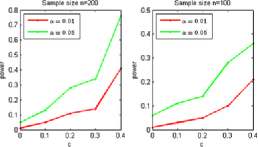
Figure 2: Plot of power curves. Rejection rates of $S_{n}$ based on the wild bootstrap method are calculated at five different values of $c$ (0, 0.1, 0.2, 0.3, and 0.4) for two sample sizes of $n$ (100 and 200) subjects at $5\%$ (green) and $1\%$ (red) significance levels.

Figure 2 depicts the power curves. It can be seen from Figure 2 that the rejection rates for $S_{n}$ based on the wild bootstrap method are accurate for moderate sample sizes, such as ($n=100$ or 200) at both significance levels ($\alpha=0.01$ or 0.05). As expected, the power increases with the sample size.

Example 2.

This example is used to evaluate the coverage probabilities of SCB of the functional coefficients ${\mathbf{B}}(s)$ based on the wild bootstrap method. The data were generated from model (26) under the same parameter values. We set $n=500$ and $M=25$, $50$, and $75$ and generated 200 datasets for each combination. Based on the generated data, we calculated SCB for each component

=250pt $\bolds{M}$ $\bolds{b_{11}}$ $\bolds{b_{12}}$ $\bolds{b_{13}}$ $\bolds{b_{21}}$ $\bolds{b_{22}}$ $\bolds{b_{23}}$ $\alpha=0.05$ $25$ 0.915 0.930 0.945 0.920 0.915 0.945 $50$ 0.925 0.940 0.945 0.930 0.925 0.950 $75$ 0.945 0.950 0.955 0.945 0.945 0.955 $\alpha=0.01$ $25$ 0.985 0.965 0.985 0.985 0.990 0.980 $50$ 0.995 0.980 0.985 0.985 0.995 0.985 $75$ 0.990 0.985 0.990 0.995 0.990 0.990

Table 1: Empirical coverage probabilities of $1-\alpha$ SCB for all components of $B_{1}(\cdot)$ and $B_{2}(\cdot)$ based on $200$ simulated data sets

of $B_{1}(s)$ and $B_{2}(s)$. Table 1 summarizes the empirical coverage probabilities based on $200$ simulations for $\alpha=0.01$ and $\alpha=0.05$. The coverage probabilities improve with the number of grid points $M$. When $M=75$, the differences between the coverage probabilities and the claimed confidence levels are fairly acceptable. The Monte Carlo errors are of size $\sqrt{0.95\times 0.05/200}\approx 0.015$ for $\alpha=0.05$. Figure 3 depicts typical simultaneous confidence bands, where $n=500$ and $M=50$. Additional simulation results are given in the supplemental article ZLK2012 .

6 Real data analysis

The data set consists of 128 healthy infants ($75$ males and $53$ females) from the neonatal project on early brain development. The gestational ages of these infants range from 262 to 433 days, and their mean gestational age is 298 days with standard deviation 17.6 days. The DTIs and T1-weighted images were acquired for each subject. For the DTIs, the imaging parameters were as follows: the six noncollinear directions at the $b$-value of 1000 s/mm² with a reference scan ($b=0$), the isotropic voxel $\mbox{resolution}=2$ mm, and the in-plane field of $\mbox{view}=256$ mm in both directions. A total of five repetitions were acquired to improve the signal-to-noise ratio of the DTIs.

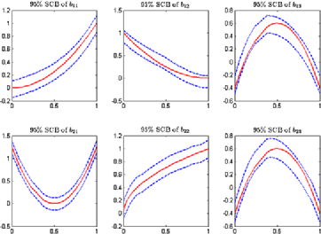
Figure 3: Typical simultaneous confidence bands with $n=500$ and $M=50$. The red solid curves are the true coefficient functions, and the blue dashed curves are the confidence bands.

The DTI data were processed by two key steps including a weighted least squares estimation method Basser1994b , Zhu2007b to construct the diffusion tensors and a DTI atlas building pipeline Goodlett2009 , Zhu2010 to register DTIs from multiple subjects to create a study specific unbiased DTI atlas, to track fiber tracts in the atlas space and to propagate them back into each subject’s native space by using registration information. Subsequently, diffusion tensors (DTs) and their scalar diffusion properties were calculated at each location along each individual fiber tract by using DTs in neighboring voxels close to the fiber tract. Figure 1(a) displays the fiber bundle of the genu of the corpus callosum (GCC), which is an area of white matter in the brain. The GCC is the anterior end of the corpus callosum, and is bent downward and backward in front of the septum pellucidum; diminishing rapidly in thickness, it is prolonged backward under the name of the rostrum, which is connected below with the lamina terminalis. It was found that neonatal microstructural development of GCC positively correlates with age and callosal thickness.

The two aims of this analysis are to compare diffusion properties including FA and MD along the GCC between the male and female groups and to delineate the development of fiber diffusion properties across time, which is addressed by including the gestational age at MRI scanning as a covariate. FA and MD, respectively, measure the inhomogeneous extent of local barriers to water diffusion and the averaged magnitude of local water diffusion. We fit model (1) to the FA and MD values from all 128 subjects, in which ${\mathbf{x}}_{i}=(1,\mathrm{G},\mathrm{Age})^{T}$, where $\mathrm{G}$ represents gender. We then applied the estimation and inference procedures to estimate ${\mathbf{B}}(s)$ and calculate $S_{n}$ for each hypothesis test. We approximated the $p$-value of $S_{n}$ using the wild bootstrap method with $G=1000$ replications. Finally, we constructed the $95\%$ simultaneous confidence bands for the functional coefficients of $B_{j}(s)$ for $j=1,2$.

Figure 4 presents the estimated coefficient functions corresponding to 1, G and Age associated with FA and MD (blue solid lines in all panels of Figure 4). The intercept functions [panels (a) and (d) in Figure 4] describe the overall trend of FA and MD. The gender coefficients for FA and MD in Figure 4(b) and (e) are negative at most of the grid points, which may indicate that compared with female infants, male infants have relatively smaller magnitudes of local water diffusivity along the genu of the corpus callosum. The gestational age coefficients for FA [panel (c) of Figure 4] are positive at most grid points, indicating that FA measures increase with age in both male and female infants, whereas those corresponding to MD [panel (f) of Figure 4] are negative at most grid points. This may indicate a negative correlation between the magnitudes of local water diffusivity and gestational age along the genu of the corpus callosum.

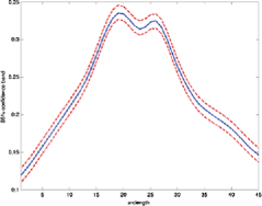
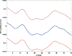
(a)	(b)
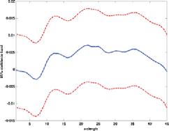
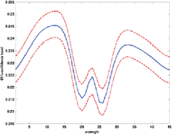
(c)	(d)
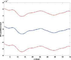
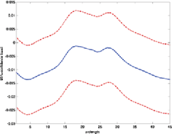
(e)	(f)

Figure 4: Plot of estimated effects of intercept [(a), (d)], gender [(b), (e)], and age [(c), (f)] and their $95\%$ confidence bands. The first three panels [(a), (b), (c)] are for FA and the last three panels [(d), (e) and (f)] are for MD. The blue solid curves are the estimated coefficient functions, and the red dashed curves are the confidence bands.

We statistically tested the effects of gender and gestational age on FA and MD along the GCC tract. To test the gender effect, we computed the global test statistic $S_{n}=144.63$ and its associated $p$-value ($p=0.078$), indicating a weakly significant gender effect, which agrees with the findings in panels (b) and (e) of Figure 4. A moderately significant age effect was found with $S_{n}=929.69$ ($p\mbox{-value}<0.001$). This agrees with the findings in panel (f) of Figure 4, indicating that MD along the GCC tract changes moderately with gestational age. Furthermore, for FA and MD, we constructed the $95\%$ simultaneous confidence bands of the varying-coefficients for G_i and age_i (Figure 4).

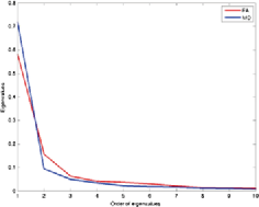
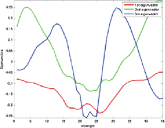
(a)	(b)
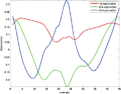
(c)

Figure 5: Plot of the first $10$ eigenvalues (a) and the first $3$ eigenfunctions for FA (b) and MD (c).

Figure 5 presents the first $10$ eigenvalues and $3$ eigenfunctions of $\hat{\Sigma}_{\eta,{jj}}(s,t)$ for $j=1,2$. The relative eigenvalues of $\hat{\Sigma}_{\eta,jj}$ defined as the ratios of the eigenvalues of $\hat{\Sigma}_{\eta,{jj}}(s,t)$ over their sum have similar distributional patterns [panel (a) of Figure 5]. We observe that the first three eigenvalues account for more than $90\%$ of the total and the others quickly vanish to zero. The eigenfunctions of FA corresponding to the largest three eigenvalues [Figure 5(b)] are different from those of MD [Figure 5(c)].

In the supplement article ZLK2012 , we further illustrate the proposed methodology by an empirical analysis of another real data set.

Appendix

We introduce some notation. We define

$$T_{B,j}(h,s) = \sum_{i=1}^{n}\sum_{m=1}^{M}K_{h}(s_{m}-s)\bigl{[}{\mathbf{x}}_{i}\otimes{\mathbf{z}}_{h}(s_{m}-s)\bigr{]}{\mathbf{x}}_{i}^{T}B_{j}(s_{m}),$$

$$T_{\eta,j}(h,s) = \sum_{i=1}^{n}\sum_{m=1}^{M}K_{h}(s_{m}-s)\bigl{[}{\mathbf{x}}_{i}\otimes{\mathbf{z}}_{h}(s_{m}-s)\bigr{]}\eta_{ij}(s_{m}),$$

$$T_{\varepsilon,j}(h,s) = \sum_{i=1}^{n}\sum_{m=1}^{M}K_{h}(s_{m}-s)\bigl{[}{\mathbf{x}}_{i}\otimes{\mathbf{z}}_{h}(s_{m}-s)\bigr{]}\varepsilon_{ij}(s_{m}),$$ (27)

$$r_{u}(K;s,h) = \frac{u_{2}(K;s,h)^{2}-u_{1}(K;s,h)u_{3}(K;s,h)}{u_{0}(K;s,h)u_{2}(K;s,h)-u_{1}(K;s,h)^{2}},$$

$$H_{h}(s_{m}-s) = K_{h}(s_{m}-s){\mathbf{z}}_{h}(s_{m}-s),$$

$$\Delta_{j}(s;{\bolds{\eta}}_{i},h_{1j}) = M^{-1}\sum_{m=1}^{M}H_{h_{1j}}(s_{m}-s)\eta_{ij}(s_{m})$$

$${}-\int_{0}^{1}H_{h_{1j}}(u-s)\eta_{ij}(u)\pi(u)\,du,$$

where $u_{r}(K;s,h)=\int_{0}^{1}h^{-r}(u-s)^{r}K_{h}(u-s)\,du$ for $r\geq 0$. Throughout the proofs, $C_{k}$’s stand for a generic constant, and it may vary from line to line.

The proofs of Theorems 1–5 rely on the following lemmas whose proofs are given in the supplemental article ZLK2012 .

Lemma 1.

Under Assumptions (C1), (C3)–(C5) and (C7), we have that for each $j$,

$$\quad\sup_{s\in[0,1]}n^{-1/2}h_{1j}\bigl{|}T_{\varepsilon,j}(h_{1j},s)\bigr{|}=O_{p}\bigl{(}\sqrt{Mh_{1j}|{\log h_{1j}}|}\bigr{)}=o_{p}(Mh_{1j}).$$ (28)

Lemma 2.

Under Assumptions (C1), (C4), (C5) and (C7), we have that for any $r\geq 0$ and $j$,

$$\sup_{s\in[0,1]}\biggl{|}\int K_{h_{1j}}(u-s)\frac{(u-s)^{r}}{h_{1j}^{r}}\,d\bigl{[}\Pi_{M}(u)-\Pi(u)\bigr{]}\biggr{|} = O_{p}\bigl{(}(Mh_{1j})^{-1/2}\bigr{)},$$

$$\sup_{s\in[0,1]}\biggl{|}\int K_{h_{1j}}(u-s)\frac{(u-s)^{r}}{h_{1j}^{r}}\varepsilon_{ij}(u)\,d\Pi_{M}(u)\biggr{|} = O_{p}\bigl{(}({Mh_{1j}})^{-1/2}\sqrt{|{\log h_{1j}}|}\bigr{)},$$

where $\Pi_{M}(\cdot)$ is the sampling distribution function based on ${\mathcal{S}}=\{s_{1},\ldots,s_{M}\}$, and $\Pi(\cdot)$ is the distribution function of $s_{m}$.

Lemma 3.

Under Assumptions (C2)–(C5), we have

$$\sup_{s\in[0,1]}\Biggl{|}n^{-1/2}\sum_{i=1}^{n}{\mathbf{x}}_{i}\otimes\Delta_{j}(s;{\bolds{\eta}}_{i},h_{1j})\Biggr{|}=o_{p}(1).$$ (29)

Lemma 4.

If Assumptions (C1) and (C3)–(C6) hold, then we have

$$\mathrm{E}\bigl{[}\hat{B}_{j}(s)|{\mathcal{S}}\bigr{]}-{B}_{j}(s) = 0.5h_{1j}^{2}u_{2}(K)\ddot{B}_{j}(s)\bigl{[}1+o_{p}(1)\bigr{]},$$

$$\operatorname{Var}\bigl{[}\hat{B}_{j}(s)|{\mathcal{S}}\bigr{]} = n^{-1}\Sigma_{\eta,jj}(s,s)\Omega_{X}^{-1}\bigl{[}1+o_{p}(1)\bigr{]},$$

where $e_{n}(s)=O_{p}((Mh_{1j})^{-1/2})$ with $E[e_{n}(s)]=0$.

Lemma 5.

If Assumptions (C1) and (C3)–(C6) hold, then for $s=0$ or $1$, we have

$$\mathrm{E}\bigl{[}\hat{B}_{j}(s)|{\mathcal{S}}\bigr{]}-B_{j}(s) = 0.5h_{1j}^{2}r_{u}(K;s,h_{1j})\ddot{B}_{j}(s)\bigl{[}1+o_{p}(1)\bigr{]},$$

$$\operatorname{Var}\bigl{[}\hat{B}_{j}(s)|{\mathcal{S}}\bigr{]} = n^{-1}\Sigma_{\eta,jj}(s,s)\Omega_{X}^{-1}\bigl{[}1+o_{p}(1)\bigr{]}.$$

Lemma 6.

Under Assumptions (C1)–(C9), we have

$$\sup_{(s,t)}n^{-1}\Biggl{|}\sum_{i=1}^{n}\overline{\varepsilon}_{ij}(s)\eta_{ij}(t)\Biggr{|} = O_{p}\bigl{(}n^{-1/2}(\log n)^{1/2}\bigr{)},$$

$$\sup_{(s,t)}n^{-1}\Biggl{|}\sum_{i=1}^{n}\overline{\varepsilon}_{ij}(s)\Delta\eta_{ij}(t)\Biggr{|} = O_{p}\bigl{(}n^{-1/2}(\log n)^{1/2}\bigr{)},$$

$$\sup_{s}n^{-1}\Biggl{|}\sum_{i=1}^{n}\overline{\varepsilon}_{ij}(s){\mathbf{x}}_{i}\Biggr{|} = O_{p}\bigl{(}n^{-1/2}(\log n)^{1/2}\bigr{)},$$

$$\sup_{s}n^{-1}\Biggl{|}\sum_{i=1}^{n}\Delta\eta_{ij}(s){\mathbf{x}}_{i}\Biggr{|} = O_{p}\bigl{(}n^{-1/2}(\log n)^{1/2}\bigr{)}.$$

Lemma 7.

Under Assumptions (C1)–(C9), we have

$$\sup_{(s,t)}n^{-1}\Biggl{|}\sum_{i=1}^{n}\overline{\varepsilon}_{ij}(s)\overline{\varepsilon}_{ij}(t)\Biggr{|}=O\bigl{(}(Mh_{2j})^{-1}+(\log n/n)^{1/2}\bigr{)}=o_{p}(1).$$

We present only the key steps in the proof of Theorem 1 below.

Proof of Theorem 1 Define

$${\mathbf{U}}_{2}(K;s,{\mathbf{H}}) = \operatorname{diag}\bigl{(}r_{u}(K;s,h_{11}),\ldots,r_{u}(K;s,h_{1J})\bigr{)},$$

$$X_{n}(s) = \sqrt{n}\bigl{\{}\hat{\mathbf{B}}(s)-E\bigl{[}\hat{\mathbf{B}}(s)|{\mathcal{S}}\bigr{]}\bigr{\}},$$

$$X_{n,j}(s) = \sqrt{n}\bigl{\{}\hat{B}_{j}(s)-E\bigl{[}\hat{B}_{j}(s)|{\mathcal{S}}\bigr{]}\bigr{\}}.$$

According to the definition of $\operatorname{vec}(\hat{A}_{j}(s))$, it is easy to see that

$$\qquad\operatorname{vec}\bigl{(}\hat{A}_{j}(s)\bigr{)} = \Sigma(s,h_{1j})^{-1}\bigl{[}T_{B,j}(h_{1j},s)+T_{\varepsilon,j}(h_{1j},s)+T_{\eta,j}(h_{1j},s)\bigr{]},$$ (32)

$$X_{n,j}(s) = \sqrt{n}\bigl{[}{\mathbf{I}}_{p}\otimes(1,0)\bigr{]}\Sigma(s,h_{1j})^{-1}\bigl{[}T_{\varepsilon,j}(h_{1j},s)+T_{\eta,j}(h_{1j},s)\bigr{]}.$$ (33)

The proof of Theorem 1(i) consists of two parts:

• Part 1 shows that $\sqrt{n}\Sigma(s,h_{1j})^{-1}T_{\varepsilon,j}(h_{1j},s)=o_{p}(1)$ holds uniformly for all $s\in[0,1]$ and $j=1,\ldots,J$.

• Part 2 shows that $\sqrt{n}\Sigma(s,h_{1j})^{-1}T_{\eta,j}(h_{1j},s)$ converges weakly to a Gaussian process $G(\cdot)$ with mean zero and covariance matrix $\Sigma_{\eta,jj}(s,s^{\prime})\Omega_{X}^{-1}$ for each $j$.

In part 1, we show that

$$\sqrt{n}\bigl{[}{\mathbf{I}}_{p}\otimes(1,0)\bigr{]}\Sigma(s,h_{1j})^{-1}T_{\varepsilon,j}(h_{1j},s)=o_{p}(1).$$ (34)

It follows from Lemma 1 that

$${n^{-1/2}}\sum_{i=1}^{n}{\mathbf{x}}_{i}\otimes\Biggl{\{}M^{-1}\sum_{m=1}^{M}K_{h_{1j}}(s_{m}-s){\mathbf{z}}_{h_{1j}}(s)\varepsilon_{i,j}(s_{m})\Biggr{\}}=o_{p}(1)$$

hold uniformly for all $s\in[0,1]$. It follows from Lemma 2 that

$$(nM)^{-1}\Sigma(s,h_{1j})=\Omega_{X}\otimes\Omega_{1}(h_{1j},s)+o_{p}(1)$$ (35)

hold uniformly for all $s\in[0,1]$. Based on these results, we can finish the proof of (34).

In part 2, we show the weak convergence of $\sqrt{n}[{\mathbf{I}}_{p}\otimes(1,0)]\Sigma(s,h_{1j})^{-1}\*T_{\eta,j}(h_{1j},s)$ for $j=1,\ldots,J$. Part 2 consists of two steps. In Step 1, it follows from the standard central limit theorem that for each $s\in[0,1]$,

$$\qquad\sqrt{n}\bigl{[}{\mathbf{I}}_{p}\otimes(1,0)\bigr{]}\Sigma(s,h_{1j})^{-1}T_{\eta,j}(h_{1j},s)\rightarrow^{L}N\bigl{(}{\mathbf{0}},\Sigma_{\eta,jj}(s,s)\Omega_{X}^{-1}\bigr{)},$$ (36)

where $\rightarrow^{L}$ denotes convergence in distribution.

Step 2 shows the asymptotic tightness of $\sqrt{n}[{\mathbf{I}}_{p}\otimes(1,0)]\Sigma(s,h_{1j})^{-1}\*T_{\eta,j}(h_{1j},s)$. By using (35) and (Appendix), $\sqrt{n}\Sigma(s,h_{1j})^{-1}T_{\eta,j}(h_{1j},s)[1+o_{p}(1)]$ can be approximated by the sum of three terms (I), (II) and (III) as follows:

(I) $$= {n^{-1/2}}\sum_{i=1}^{n}\Omega_{X}^{-1}{\mathbf{x}}_{i}\otimes\Omega_{1}(h_{1j},s)^{-1}\Delta_{j}(s;{\bolds{\eta}}_{i},h_{1j}),$$

(II) $$= {n^{-1/2}}\sum_{i=1}^{n}\Omega_{X}^{-1}{\mathbf{x}}_{i}\otimes\Omega_{1}(h_{1j},s)^{-1}\eta_{ij}(s)$$

$${}\times\int_{\max(-sh_{1j}^{-1},-1)}^{\min((1-s)h_{1j}^{-1},1)}K(u)(1,u)^{T}\pi(s+h_{1j}u)\,du,$$

(III) $$= {n^{-1/2}}\sum_{i=1}^{n}\Omega_{X}^{-1}{\mathbf{x}}_{i}\otimes\Omega_{1}(h_{1j},s)^{-1}$$

$$\hskip 40.0pt{}\times\int_{\max(-sh_{1j}^{-1},-1)}^{\min((1-s)h_{1j}^{-1},1)}K(u)\pmatrix{1\cr u}\bigl{[}\eta_{ij}(s+h_{1j}u)-\eta_{ij}(s)\bigr{]}$$

$$\hskip 40.0pt\qquad\quad\hskip 51.0pt{}\times\pi(s+h_{1j}u)\,du.$$

We investigate the three terms on the right-hand side of (Appendix) as follows. It follows from Lemma 3 that the first term on the right-hand side of (Appendix) converges to zero uniformly. We prove the asymptotic tightness of (II) as follows. Define

$$\hat{X}_{n,j}(s) = {n^{-1/2}}\sum_{i=1}^{n}\Omega_{X}^{-1}{\mathbf{x}}_{i}\otimes(1,0)\Omega_{1}(h_{1j},s)^{-1}\eta_{ij}(s)$$

$${}\times\int_{\max(-sh_{1j}^{-1},-1)}^{\min((1-s)h_{1j}^{-1},1)}K(u)(1,u)^{T}\pi(s+h_{1j}u)\,du.$$

Thus, we only need to prove the asymptotic tightness of $\hat{X}_{n,j}(s)$. The asymptotic tightness of $\hat{X}_{n,j}(s)$ can be proved using the empirical process techniques VaartWellner1996 . It follows that

$$(1,0)\Omega_{1}(h_{1j},s)^{-1}\int_{\max(-sh_{1j}^{-1},-1)}^{\min((1-s)h_{1j}^{-1},1)}K(u)(1,u)^{T}\pi(s+h_{1j}u)\,du$$

$$\qquad=\frac{u_{2}(K;s,h_{1j})u_{0}(K;s,h_{1j})-u_{1}(K;s,h_{1j})^{2}+o(h_{1j})}{u_{2}(K;s,h_{1j})u_{0}(K;s,h_{1j})-u_{1}(K;s,h_{1j})^{2}+o(h_{1j})}=1+o(h_{1j}).$$

Thus, $\hat{X}_{n,j}(s)$ can be simplified as

$$\hat{X}_{n,j}(s)=\bigl{[}1+o(h_{1j})\bigr{]}{n^{-1/2}}\sum_{i=1}^{n}\eta_{ij}(s)\Omega_{X}^{-1}{\mathbf{x}}_{i}.$$

We consider a function class ${\mathcal{E}}_{\eta}=\{f(s;{\mathbf{x}},\eta_{\cdot,j})=\Omega_{X}^{-1}{\mathbf{x}}\eta_{\cdot,j}(s)\dvtx s\in[0,1]\}$. Due to Assumption (C2), ${\mathcal{E}}_{\eta}$ is a $P$-Donsker class.

Finally, we consider the third term (III) on the right-hand side of (Appendix). It is easy to see that (III) can be written as

$$\Omega_{X}^{-1}\otimes\Omega_{1}(h_{1j},s)^{-1}$$

$$\qquad{}\times\int_{\max(-sh_{1j}^{-1},-1)}^{\min((1-s)h_{1j}^{-1},1)}K(u)\Biggl{[}{n^{-1/2}}\sum_{i=1}^{n}{\mathbf{x}}_{i}\bigl{\{}\eta_{ij}(s+h_{1j}u)-\eta_{ij}(s)\bigr{\}}\Biggr{]}\otimes\pmatrix{1\cr u}$$

$$\hskip 83.2pt\qquad{}\times\pi(s+h_{1j}u)\,du.$$

Using the same argument of proving the second term (II), we can show the asymptotic tightness of ${n^{-1/2}}\sum_{i=1}^{n}{\mathbf{x}}_{i}\eta_{ij}(s)$. Therefore, for any $h_{1j}\rightarrow 0$,

$$\sup_{s\in[0,1],|u|\leq 1}\Biggl{|}n^{-1/2}\sum_{i=1}^{n}{\mathbf{x}}_{i}\bigl{\{}\eta_{ij}(s+h_{1j}u)-\eta_{ij}(s)\bigr{\}}\Biggr{|}=o_{p}(1).$$ (38)

It follows from Assumptions (C5) and (C7) and (38) that (III) converges to zero uniformly. Therefore, we can finish the proof of Theorem 1(i). Since Theorem 1(ii) is a direct consequence of Theorem 1(i) and Lemma 4, we finish the proof of Theorem 1.

Proof of Theorem 2 Proofs of parts (a)–(d) are completed by some straightforward calculations. Detailed derivation is given in the supplemental document. Here we prove part (e) only. Let $\tilde{K}_{M,h}(s)=\tilde{K}_{M}(s/h)/h$, where $\tilde{K}_{M}(s)$ is the empirical equivalent kernels for the first-order local polynomial kernel Fan1996 . Thus, we have

$$\quad\hat{\eta}_{ij}(s)-\eta_{ij}(s) = \sum_{m=1}^{M}\tilde{K}_{M,h_{2j}}(s_{m}-s){\mathbf{x}}_{i}^{T}\bigl{[}B_{j}(s_{m})-\hat{B}_{j}(s_{m})\bigr{]}$$

$${}+\sum_{m=1}^{M}\tilde{K}_{M,h_{2j}}(s_{m}-s)\bigl{[}\eta_{ij}(s_{m})+\varepsilon_{ij}(s_{m})-\eta_{ij}(s)\bigr{]}.$$

We define

$$\overline{\varepsilon}_{ij}(s) = \sum_{m=1}^{M}\tilde{K}_{M,h_{2j}}(s_{m}-s)\varepsilon_{ij}(s_{m}),$$

$$\Delta\eta_{ij}(s) = \sum_{m=1}^{M}\tilde{K}_{M,h_{2j}}(s_{m}-s)\bigl{[}\eta_{ij}(s_{m})-\eta_{ij}(s)\bigr{]},$$

$$\Delta B_{j}(s) = \sum_{m=1}^{M}\tilde{K}_{M,h_{2j}}(s_{m}-s)\bigl{[}B_{j}(s_{m})-\hat{B}_{j}(s_{m})\bigr{]},$$

$$\Delta_{ij}(s) = \overline{\varepsilon}_{ij}(s)+\Delta\eta_{ij}(s)+{\mathbf{x}}_{i}^{T}\Delta B_{j}(s).$$

It follows from (Appendix) that

$$\hat{\eta}_{ij}(s)-\eta_{ij}(s)=\Delta_{ij}(s)=\overline{\varepsilon}_{ij}(s)+\Delta\eta_{ij}(s)+{\mathbf{x}}_{i}^{T}\Delta B_{j}(s).$$ (40)

It follows from Lemma 2 and a Taylor expansion that

$$\sup_{s\in[0,1]}\bigl{|}\overline{\varepsilon}_{ij}(s)\bigr{|}=O_{p}\biggl{(}\sqrt{\frac{|{\log(h_{2j})}|}{Mh_{2j}}}\biggr{)}$$

and

$$\sup_{s\in[0,1]}\bigl{|}\Delta\eta_{ij}(s)\bigr{|}=O_{p}(1)\sup_{s\in[0,1]}\bigl{|}\ddot{\eta}_{ij}(s)\bigr{|}h_{1j}^{(2)2}.$$

Since $\sqrt{n}\{\hat{B}_{j}(\cdot)-B_{j}(\cdot)-0.5u_{2}(K)^{2}h_{1j}^{2}\ddot{B}_{j}(\cdot)[1+o_{p}(1)]\}$ weakly converges to a Gaussian process in $\ell^{\infty}([0,1])$ as $n\rightarrow\infty$, $\sqrt{n}\{\hat{B}_{j}(\cdot)-B_{j}(\cdot)-0.5u_{2}(K)^{2}h_{1j}^{2}\*\ddot{B}_{j}(\cdot)[1+o_{p}(1)]\}$ is asymptotically tight. Thus, we have

$$\Delta B_{ij}(s) = -\sum_{m=1}^{M}\tilde{K}_{M,h_{2j}}(s_{j}-s)0.5u_{2}(K)^{2}h_{1j}^{2}\ddot{B}_{j}(s_{m})\bigl{[}1+o_{p}(1)\bigr{]}$$

$${}+\sum_{m=1}^{M}\tilde{K}_{M,h_{2j}}(s_{j}-s)\bigl{\{}0.5u_{2}(K)^{2}h_{1j}^{2}\ddot{B}_{j}(s_{m})\bigl{[}1+o_{p}(1)\bigr{]}$$

$$\hskip 160.2pt{}+B_{j}(s_{m})-\hat{B}_{j}(s_{m})\bigr{\}},$$

$$\sup_{s\in[0,1]}\bigl{\|}\Delta B_{j}(s)\bigr{\|} = O_{p}\bigl{(}n^{-1/2}\bigr{)}+O_{p}\bigl{(}h_{1j}^{2}\bigr{)}.$$

Combining these results, we have

$$\sup_{s\in[0,1]}\bigl{|}\hat{\eta}_{ij}(s)-\eta_{ij}(s)\bigr{|}=O_{p}\bigl{(}{\bigl{|}\log(h_{2j})\bigr{|}}^{1/2}({Mh_{2j}})^{-1/2}+h_{1j}^{(2)2}+h_{1j}^{2}+n^{-1/2}\bigr{)}.$$

This completes the proof of part (e).

Proof of Theorem 3 Recall that $\hat{\eta}_{ij}(s)=\eta_{ij}(s)+\Delta_{i,j}(s)$, we have

$$\qquad n^{-1}\sum_{i=1}^{n}\hat{\eta}_{ij}(s)\hat{\eta}_{ij}(t) = n^{-1}\sum_{i=1}^{n}\Delta_{ij}(s)\Delta_{ij}(t)+n^{-1}\sum_{i=1}^{n}\eta_{ij}(s)\Delta_{ij}(t)$$

$${}+n^{-1}\sum_{i=1}^{n}\Delta_{ij}(s)\eta_{ij}(t)+n^{-1}\sum_{i=1}^{n}\eta_{ij}(s)\eta_{ij}(t).$$

This proof consists of two steps. The first step is to show that the first three terms on the right-hand side of (Appendix) converge to zero uniformly for all $(s,t)\in[0,1]^{2}$ in probability. The second step is to show the uniform convergence of $n^{-1}\sum_{i=1}^{n}\eta_{ij}(s)\eta_{ij}(t)$ to $\Sigma_{\eta}(s,t)$ over $(s,t)\in[0,1]^{2}$ in probability.

We first show that

$$\qquad\sup_{(s,t)}n^{-1}\Biggl{|}\sum_{i=1}^{n}\Delta_{ij}(s)\eta_{ij}(t)\Biggr{|}=O_{p}\bigl{(}n^{-1/2}+h_{1j}^{2}+h_{2j}^{2}+(\log n/n)^{1/2}\bigr{)}.$$ (42)

Since

$$\sum_{i=1}^{n}\Delta_{ij}(s)\eta_{ij}(t)$$

$$\qquad\leq n^{-1}\Biggl{\{}\Biggl{|}\sum_{i=1}^{n}\overline{\varepsilon}_{ij}(s)\eta_{ij}(t)\Biggr{|}+\Biggl{|}\sum_{i=1}^{n}\Delta\eta_{ij}(s)\eta_{ij}(t)\Biggr{|}$$ (43)

$$\qquad\quad\hskip 85.0pt{}+\Biggl{|}\sum_{i=1}^{n}{\mathbf{x}}_{i}^{T}\Delta B_{j}(s)\eta_{ij}(t)\Biggr{|}\Biggr{\}},$$

it is sufficient to focus on the three terms on the right-hand side of (Appendix). Since

$$\bigl{|}{\mathbf{x}}_{i}^{T}\Delta B_{j}(s)\eta_{ij}(t)\bigr{|}\leq\|{\mathbf{x}}_{i}\|_{2}\sup_{s\in[0,1]}\bigl{\|}\Delta B_{k}(s)\bigr{\|}_{2}\sup_{t\in[0,1]}\bigl{|}\eta_{ij}(t)\bigr{|},$$

we have

$$n^{-1}\Biggl{|}\sum_{i=1}^{n}{\mathbf{x}}_{i}^{T}\Delta B_{j}(s)\eta_{ij}(t)\Biggr{|} \leq \sup_{s\in[0,1]}\bigl{\|}\Delta B_{k}(s)\bigr{\|}_{2}n^{-1}\sum_{i=1}^{n}\|{\mathbf{x}}_{i}\|_{2}\bigl{|}\eta_{ij}(t)\bigr{|}$$

$$= O_{p}\bigl{(}n^{-1/2}+h_{1j}^{2}\bigr{)}.$$

Similarly, we have

$$n^{-1}\Biggl{|}\sum_{i=1}^{n}\Delta\eta_{ij}(s)\eta_{ij}(t)\Biggr{|}\leq n^{-1}\sum_{i=1}^{n}\sup_{s,t\in[0,1]}\bigl{|}\Delta\eta_{ij}(s)\eta_{ij}(t)\bigr{|}=O_{p}\bigl{(}h_{1j}^{(2)2}\bigr{)}=o_{p}(1).$$

It follows from Lemma 6 that $\sup_{(s,t)}n^{-1}\{|\sum_{i=1}^{n}\overline{\varepsilon}_{ij}(s)\eta_{ij}(t)|=O((\log n/n)^{1/2})$. Similarly, we can show that $\sup_{(s,t)}n^{-1}|\sum_{i=1}^{n}\Delta_{ij}(t)\eta_{ij}(s)|=O_{p}(n^{-1/2}+h_{1j}^{2}+h_{2j}^{2}+(\log n/n)^{1/2})$.

We can show that

$$\sup_{(s,t)}\Biggl{|}n^{-1}\sum_{i=1}^{n}\bigl{[}\eta_{ij}(s)\eta_{ij}(t)-\Sigma_{\eta,jj}(s,t)\bigr{]}\Biggr{|}=O_{p}\bigl{(}n^{-1/2}\bigr{)}.$$ (44)

Note that

$$\bigl{|}\eta_{ij}(s_{1})\eta_{ij}(t_{1})-\eta_{ij}(s_{2})\eta_{ij}(t_{2})\bigr{|}$$

$$\qquad\leq 2\bigl{(}|s_{1}-s_{2}|+|t_{1}-t_{2}|\bigr{)}\sup_{s\in[0,1]}\bigl{|}\dot{\eta}_{ij}(s)\bigr{|}\sup_{s\in[0,1]}\bigl{|}\eta_{ij}(s)\bigr{|}$$

holds for any $(s_{1},t_{1})$ and $(s_{2},t_{2})$, the functional class $\{\eta_{j}(u)\eta_{j}(v)\dvtx(u,v)\in[0,1]^{2}\}$ is a Vapnik and Cervonenkis (VC) class VaartWellner1996 , Kosorok2008 . Thus, it yields that (44) is true.

Finally, we can show that

$$\sup_{(s,t)}n^{-1}\Biggl{|}\sum_{i=1}^{n}\Delta_{ij}(s)\Delta_{ij}(t)\Biggr{|}$$

(45)

$$\qquad=O_{p}\bigl{(}(Mh_{2j})^{-1}+(\log n/n)^{1/2}+h^{4}_{j}+h_{1j}^{(2)4}\bigr{)}.$$

With some calculations, for a positive constant $C_{1}$, we have

$$\Biggl{|}\sum_{i=1}^{n}\Delta_{ij}(s)\Delta_{ij}(t)\Biggr{|}$$

$$\qquad\leq C_{1}\sup_{(s,t)}\Biggl{[}\Biggl{|}\sum_{i=1}^{n}\overline{\varepsilon}_{ij}(s)\overline{\varepsilon}_{ij}(t)\Biggr{|}+\Biggl{|}\sum_{i=1}^{n}\overline{\varepsilon}_{ij}(s)\Delta\eta_{ij}(t)\Biggr{|}$$

$$\hskip 34.0pt\qquad\quad{}+\Biggl{|}\sum_{i=1}^{n}\Delta\eta_{ij}(t){\mathbf{x}}_{i}^{T}\Delta B_{j}(s)\Biggr{|}+\Biggl{|}\sum_{i=1}^{n}\overline{\varepsilon}_{ij}(s){\mathbf{x}}_{i}^{T}\Delta B_{j}(t)\Biggr{|}$$

$$\hskip 34.0pt\qquad\quad{}+\Biggl{|}\sum_{i=1}^{n}\Delta\eta_{ij}(s)\Delta\eta_{ij}(t)\Biggr{|}+\Biggl{|}\sum_{i=1}^{n}{\mathbf{x}}_{i}^{T}\Delta B_{j}(s)\Delta B_{j}(t){\mathbf{x}}_{i}\Biggr{|}\Biggr{]}.$$

It follows from Lemma 7 that

$$\sup_{(s,t)}n^{-1}\Biggl{|}\sum_{i=1}^{n}\overline{\varepsilon}_{ij}(s)\overline{\varepsilon}_{ij}(t)\Biggr{|} = O_{p}\bigl{(}(Mh_{2j})^{-1}+(\log n/n)^{1/2}\bigr{)},$$

$$\sup_{(s,t)}n^{-1}\Biggl{[}\Biggl{|}\sum_{i=1}^{n}\overline{\varepsilon}_{ij}(s)\Delta\eta_{ij}(t)\Biggr{|}+\Biggl{|}\sum_{i=1}^{n}\Delta\eta_{ij}(t){\mathbf{x}}_{i}^{T}\Delta B_{j}(s)\Biggr{|}+\Biggl{|}\sum_{i=1}^{n}\overline{\varepsilon}_{ij}(s){\mathbf{x}}_{i}^{T}\Delta B_{j}(t)\Biggr{|}\Biggr{]}$$

$$\qquad=O_{p}\bigl{(}(\log n/n)^{1/2}\bigr{)}.$$

Since $\sup_{s\in[0,1]}|\Delta\eta_{ij}(s)|=C_{2}\sup_{s\in[0,1]}|\ddot{\eta}_{ij}(s)|h_{2j}^{2},$ we have

$$\sup_{(s,t)}n^{-1}\Biggl{|}\sum_{i=1}^{n}\Delta\eta_{ij}(s)\Delta\eta_{ij}(t)\Biggr{|}=O\bigl{(}h_{1j}^{(2)4}\bigr{)}.$$

Furthermore, since $\sup_{s\in[0,1]}\|\Delta{\mathbf{B}}(s)\|=O_{p}(n^{-1/2}+h^{2}_{j})$, we have

$$n^{-1}\Biggl{|}\sum_{i=1}^{n}{\mathbf{x}}_{i}^{T}\Delta B_{j}(s)\Delta B_{j}(t){\mathbf{x}}_{i}\Biggr{|}=O_{p}\bigl{(}n^{-1}+h^{4}_{j}\bigr{)}.$$

Note that the arguments for (42)–(Appendix) hold for $\hat{\Sigma}_{\eta,jj^{\prime}}(\cdot,\cdot)$ for any $j\not=j^{\prime}$. Thus, combining (42)–(Appendix) leads to Theorem 3(i).

To prove Theorem 3(ii), we follow the same arguments in Lemma 6 of Li and Hsing LiHsing2010 . For completion, we highlight several key steps below. We define

$$(\Delta\psi_{j,j})(s)=\int_{0}^{1}\bigl{[}\hat{\Sigma}_{\eta,jj}(s,t)-\Sigma_{\eta,jj}(s,t)\bigr{]}\psi_{j,j}(t)\,dt.$$ (46)

Following Hall and Hosseini-Nasab HallHosseini2006 and the Cauchy–Schwarz inequality, we have

$$\biggl{\{}\int_{0}^{1}\bigl{[}\hat{\psi}_{j,j}(s)-\psi_{j,j}(s)\bigr{]}^{2}\,ds\biggr{\}}^{1/2}$$

$$\qquad\leq C_{2}\biggl{\{}\biggl{[}\int_{0}^{1}(\Delta\psi_{j,j})(s)^{2}\,ds\biggr{]}^{1/2}+\int_{0}^{1}\int_{0}^{1}\bigl{[}\hat{\Sigma}_{\eta,jj}(s,t)-\Sigma_{\eta,jj}(s,t)\bigr{]}^{2}\,ds\,dt\biggr{\}}$$

$$\qquad\leq C_{2}\biggl{\{}\int_{0}^{1}\int_{0}^{1}\bigl{[}\hat{\Sigma}_{\eta,jj}(s,t)-\Sigma_{\eta,jj}(s,t)\bigr{]}^{2}\,ds\,dt\biggr{\}}^{1/2}\biggl{\{}\int_{0}^{1}\bigl{[}\psi_{j,j}(t)\bigr{]}^{2}\,dt\biggr{\}}^{1/2}$$

$$\qquad\quad{}+\int_{0}^{1}\int_{0}^{1}\bigl{[}\hat{\Sigma}_{\eta,jj}(s,t)-\Sigma_{\eta,jj}(s,t)\bigr{]}^{2}\,ds\,dt$$

$$\qquad\leq C_{3}\sup_{(s,t)\in[0,1]^{2}}\bigl{|}\hat{\Sigma}_{\eta,jj}(s,t)-\Sigma_{\eta,jj}(s,t)\bigr{|},$$

which yields Theorem 3(ii)(a).

Using (4.9) in Hall, Müller and Wang MR2278365 , we have

$$|\hat{\lambda}_{j,j}-\lambda_{j,j}|$$

$$\qquad\leq|\int_{0}^{1}\int_{0}^{1}[\hat{\Sigma}_{\eta,jj}-\Sigma_{\eta,jj}](s,t)\psi_{j,j}(s)\psi_{j,j}(t)\,ds\,dt$$

$$\qquad\quad{}+O\biggl{(}\int_{0}^{1}(\Delta\psi_{j,j})(s)^{2}\,ds\biggr{)}$$

$$\qquad\leq C_{4}\sup_{(s,t)\in[0,1]^{2}}\bigl{|}\hat{\Sigma}_{\eta,jj}(s,t)-\Sigma_{\eta,jj}(s,t)\bigr{|},$$

which yields Theorem 3(ii)(b). This completes the proof.

Proof of Theorem 5 The proof of Theorem 5 is given in the supplement arctile ZLK2012 .

References

- (1) {barticle}[pbm] \bauthor\bsnmAguirre, \bfnmG. K.\binitsG. K., \bauthor\bsnmZarahn, \bfnmE.\binitsE. and \bauthor\bsnmD’esposito, \bfnmM.\binitsM. (\byear1998). \btitleThe variability of human, BOLD hemodynamic responses. \bjournalNeuroImage \bvolume8 \bpages360–369. \biddoi=10.1006/nimg.1998.0369, issn=1053-8119, pii=S1053-8119(98)90369-X, pmid=9811554 \bptokimsref \endbibitem
- (2) {barticle}[author] \bauthor\bsnmBasser, \bfnmP. J.\binitsP. J., \bauthor\bsnmMattiello, \bfnmJ.\binitsJ. and \bauthor\bsnmLeBihan, \bfnmD.\binitsD. (\byear1994). \btitleEstimation of the effective self- diffusion tensor from the NMR spin echo. \bjournalJournal of Magnetic Resonance Ser. B \bvolume103 \bpages247–254. \bptokimsref \endbibitem
- (3) {barticle}[pbm] \bauthor\bsnmBasser, \bfnmP. J.\binitsP. J., \bauthor\bsnmMattiello, \bfnmJ.\binitsJ. and \bauthor\bsnmLeBihan, \bfnmD.\binitsD. (\byear1994). \btitleMR diffusion tensor spectroscopy and imaging. \bjournalBiophys. J. \bvolume66 \bpages259–267. \biddoi=10.1016/S0006-3495(94)80775-1, issn=0006-3495, pii=S0006-3495(94)80775-1, pmcid=1275686, pmid=8130344 \bptokimsref \endbibitem
- (4) {bbook}[mr] \bauthor\bsnmBuzsáki, \bfnmGyörgy\binitsG. (\byear2006). \btitleRhythms of the Brain. \bpublisherOxford Univ. Press, \blocationOxford. \biddoi=10.1093/acprof:oso/9780195301069.001.0001, mr=2270828 \bptokimsref \endbibitem
- (5) {barticle}[mr] \bauthor\bsnmCardot, \bfnmHervé\binitsH. (\byear2007). \btitleConditional functional principal components analysis. \bjournalScand. J. Stat. \bvolume34 \bpages317–335. \biddoi=10.1111/j.1467-9469.2006.00521.x, issn=0303-6898, mr=2346642 \bptokimsref \endbibitem
- (6) {barticle}[mr] \bauthor\bsnmCardot, \bfnmHervé\binitsH., \bauthor\bsnmChaouch, \bfnmMohamed\binitsM., \bauthor\bsnmGoga, \bfnmCamelia\binitsC. and \bauthor\bsnmLabruère, \bfnmCatherine\binitsC. (\byear2010). \btitleProperties of design-based functional principal components analysis. \bjournalJ. Statist. Plann. Inference \bvolume140 \bpages75–91. \biddoi=10.1016/j.jspi.2009.06.012, issn=0378-3758, mr=2568123 \bptokimsref \endbibitem
- (7) {barticle}[mr] \bauthor\bsnmCardot, \bfnmHervé\binitsH. and \bauthor\bsnmJosserand, \bfnmEtienne\binitsE. (\byear2011). \btitleHorvitz–Thompson estimators for functional data: Asymptotic confidence bands and optimal allocation for stratified sampling. \bjournalBiometrika \bvolume98 \bpages107–118. \biddoi=10.1093/biomet/asq070, issn=0006-3444, mr=2804213 \bptokimsref \endbibitem
- (8) {barticle}[mr] \bauthor\bsnmChiou, \bfnmJeng-Min\binitsJ.-M., \bauthor\bsnmMüller, \bfnmHans-Georg\binitsH.-G. and \bauthor\bsnmWang, \bfnmJane-Ling\binitsJ.-L. (\byear2004). \btitleFunctional response models. \bjournalStatist. Sinica \bvolume14 \bpages675–693. \bidissn=1017-0405, mr=2087968 \bptokimsref \endbibitem
- (9) {barticle}[mr] \bauthor\bsnmDegras, \bfnmDavid A.\binitsD. A. (\byear2011). \btitleSimultaneous confidence bands for nonparametric regression with functional data. \bjournalStatist. Sinica \bvolume21 \bpages1735–1765. \biddoi=10.5705/ss.2009.207, issn=1017-0405, mr=2895997 \bptokimsref \endbibitem
- (10) {barticle}[mr] \bauthor\bsnmEinmahl, \bfnmUwe\binitsU. and \bauthor\bsnmMason, \bfnmDavid M.\binitsD. M. (\byear2000). \btitleAn empirical process approach to the uniform consistency of kernel-type function estimators. \bjournalJ. Theoret. Probab. \bvolume13 \bpages1–37. \biddoi=10.1023/A:1007769924157, issn=0894-9840, mr=1744994 \bptokimsref \endbibitem
- (11) {bbook}[mr] \bauthor\bsnmFan, \bfnmJ.\binitsJ. and \bauthor\bsnmGijbels, \bfnmI.\binitsI. (\byear1996). \btitleLocal Polynomial Modelling and Its Applications. \bseriesMonographs on Statistics and Applied Probability \bvolume66. \bpublisherChapman & Hall, \blocationLondon. \bidmr=1383587 \bptokimsref \endbibitem
- (12) {barticle}[mr] \bauthor\bsnmFan, \bfnmJianqing\binitsJ., \bauthor\bsnmYao, \bfnmQiwei\binitsQ. and \bauthor\bsnmCai, \bfnmZongwu\binitsZ. (\byear2003). \btitleAdaptive varying-coefficient linear models. \bjournalJ. R. Stat. Soc. Ser. B Stat. Methodol. \bvolume65 \bpages57–80. \biddoi=10.1111/1467-9868.00372, issn=1369-7412, mr=1959093 \bptokimsref \endbibitem
- (13) {barticle}[mr] \bauthor\bsnmFan, \bfnmJianqing\binitsJ. and \bauthor\bsnmZhang, \bfnmWenyang\binitsW. (\byear1999). \btitleStatistical estimation in varying coefficient models. \bjournalAnn. Statist. \bvolume27 \bpages1491–1518. \biddoi=10.1214/aos/1017939139, issn=0090-5364, mr=1742497 \bptokimsref \endbibitem
- (14) {barticle}[mr] \bauthor\bsnmFan, \bfnmJianqing\binitsJ. and \bauthor\bsnmZhang, \bfnmWenyang\binitsW. (\byear2000). \btitleSimultaneous confidence bands and hypothesis testing in varying-coefficient models. \bjournalScand. J. Stat. \bvolume27 \bpages715–731. \biddoi=10.1111/1467-9469.00218, issn=0303-6898, mr=1804172 \bptokimsref \endbibitem
- (15) {barticle}[mr] \bauthor\bsnmFan, \bfnmJianqing\binitsJ. and \bauthor\bsnmZhang, \bfnmWenyang\binitsW. (\byear2008). \btitleStatistical methods with varying coefficient models. \bjournalStat. Interface \bvolume1 \bpages179–195. \bidissn=1938-7989, mr=2425354 \bptokimsref \endbibitem
- (16) {barticle}[mr] \bauthor\bsnmFaraway, \bfnmJulian J.\binitsJ. J. (\byear1997). \btitleRegression analysis for a functional response. \bjournalTechnometrics \bvolume39 \bpages254–261. \biddoi=10.2307/1271130, issn=0040-1706, mr=1462586 \bptokimsref \endbibitem
- (17) {barticle}[pbm] \bauthor\bsnmFass, \bfnmLeonard\binitsL. (\byear2008). \btitleImaging and cancer: A review. \bjournalMol. Oncol. \bvolume2 \bpages115–152. \biddoi=10.1016/j.molonc.2008.04.001, issn=1878-0261, pii=S1574-7891(08)00059-8, pmid=19383333 \bptokimsref \endbibitem
- (18) {bbook}[author] \bauthor\bsnmFriston, \bfnmK. J.\binitsK. J. (\byear2007). \btitleStatistical Parametric Mapping: The Analysis of Functional Brain Images. \bpublisherAcademic Press, \blocationLondon. \bptokimsref \endbibitem
- (19) {barticle}[pbm] \bauthor\bsnmFriston, \bfnmKarl J.\binitsK. J. (\byear2009). \btitleModalities, modes, and models in functional neuroimaging. \bjournalScience \bvolume326 \bpages399–403. \biddoi=10.1126/science.1174521, issn=1095-9203, pii=326/5951/399, pmid=19833961 \bptokimsref \endbibitem
- (20) {barticle}[pbm] \bauthor\bsnmGoodlett, \bfnmCasey B.\binitsC. B., \bauthor\bsnmFletcher, \bfnmP. Thomas\binitsP. T., \bauthor\bsnmGilmore, \bfnmJohn H.\binitsJ. H. and \bauthor\bsnmGerig, \bfnmGuido\binitsG. (\byear2009). \btitleGroup analysis of DTI fiber tract statistics with application to neurodevelopment. \bjournalNeuroImage \bvolume45 \bpagesS133–S142. \biddoi=10.1016/j.neuroimage.2008.10.060, issn=1095-9572, mid=NIHMS100396, pii=S1053-8119(08)01199-3, pmcid=2727755, pmid=19059345 \bptokimsref \endbibitem
- (21) {barticle}[mr] \bauthor\bsnmHall, \bfnmPeter\binitsP. and \bauthor\bsnmHosseini-Nasab, \bfnmMohammad\binitsM. (\byear2006). \btitleOn properties of functional principal components analysis. \bjournalJ. R. Stat. Soc. Ser. B Stat. Methodol. \bvolume68 \bpages109–126. \biddoi=10.1111/j.1467-9868.2005.00535.x, issn=1369-7412, mr=2212577 \bptokimsref \endbibitem
- (22) {barticle}[mr] \bauthor\bsnmHall, \bfnmPeter\binitsP., \bauthor\bsnmMüller, \bfnmHans-Georg\binitsH.-G. and \bauthor\bsnmWang, \bfnmJane-Ling\binitsJ.-L. (\byear2006). \btitleProperties of principal component methods for functional and longitudinal data analysis. \bjournalAnn. Statist. \bvolume34 \bpages1493–1517. \biddoi=10.1214/009053606000000272, issn=0090-5364, mr=2278365 \bptokimsref \endbibitem
- (23) {barticle}[mr] \bauthor\bsnmHall, \bfnmPeter\binitsP., \bauthor\bsnmMüller, \bfnmHans-Georg\binitsH.-G. and \bauthor\bsnmYao, \bfnmFang\binitsF. (\byear2008). \btitleModelling sparse generalized longitudinal observations with latent Gaussian processes. \bjournalJ. R. Stat. Soc. Ser. B Stat. Methodol. \bvolume70 \bpages703–723. \biddoi=10.1111/j.1467-9868.2008.00656.x, issn=1369-7412, mr=2523900 \bptokimsref \endbibitem
- (24) {barticle}[mr] \bauthor\bsnmHastie, \bfnmTrevor\binitsT. and \bauthor\bsnmTibshirani, \bfnmRobert\binitsR. (\byear1993). \btitleVarying-coefficient models. \bjournalJ. R. Stat. Soc. Ser. B Stat. Methodol. \bvolume55 \bpages757–796. \bidissn=0035-9246, mr=1229881 \bptnotecheck related\bptokimsref \endbibitem
- (25) {bbook}[author] \bauthor\bsnmHeywood, \bfnmI.\binitsI., \bauthor\bsnmCornelius, \bfnmS.\binitsS. and \bauthor\bsnmCarver, \bfnmS.\binitsS. (\byear2006). \btitleAn Introduction to Geographical Information Systems., \bedition3rd ed. \bpublisherPrentice Hall, \blocationNew York. \bptokimsref \endbibitem
- (26) {barticle}[mr] \bauthor\bsnmHoover, \bfnmDonald R.\binitsD. R., \bauthor\bsnmRice, \bfnmJohn A.\binitsJ. A., \bauthor\bsnmWu, \bfnmColin O.\binitsC. O. and \bauthor\bsnmYang, \bfnmLi-Ping\binitsL.-P. (\byear1998). \btitleNonparametric smoothing estimates of time-varying coefficient models with longitudinal data. \bjournalBiometrika \bvolume85 \bpages809–822. \biddoi=10.1093/biomet/85.4.809, issn=0006-3444, mr=1666699 \bptokimsref \endbibitem
- (27) {barticle}[mr] \bauthor\bsnmHuang, \bfnmJianhua Z.\binitsJ. Z., \bauthor\bsnmWu, \bfnmColin O.\binitsC. O. and \bauthor\bsnmZhou, \bfnmLan\binitsL. (\byear2002). \btitleVarying-coefficient models and basis function approximations for the analysis of repeated measurements. \bjournalBiometrika \bvolume89 \bpages111–128. \biddoi=10.1093/biomet/89.1.111, issn=0006-3444, mr=1888349 \bptokimsref \endbibitem
- (28) {barticle}[mr] \bauthor\bsnmHuang, \bfnmJianhua Z.\binitsJ. Z., \bauthor\bsnmWu, \bfnmColin O.\binitsC. O. and \bauthor\bsnmZhou, \bfnmLan\binitsL. (\byear2004). \btitlePolynomial spline estimation and inference for varying coefficient models with longitudinal data. \bjournalStatist. Sinica \bvolume14 \bpages763–788. \bidissn=1017-0405, mr=2087972 \bptokimsref \endbibitem
- (29) {bbook}[author] \bauthor\bsnmHuettel, \bfnmS. A.\binitsS. A., \bauthor\bsnmSong, \bfnmA. W.\binitsA. W. and \bauthor\bsnmMcCarthy, \bfnmG.\binitsG. (\byear2004). \btitleFunctional Magnetic Resonance Imaging. \bpublisherSinauer, \blocationLondon. \bptokimsref \endbibitem
- (30) {barticle}[mr] \bauthor\bsnmKosorok, \bfnmMichael R.\binitsM. R. (\byear2003). \btitleBootstraps of sums of independent but not identically distributed stochastic processes. \bjournalJ. Multivariate Anal. \bvolume84 \bpages299–318. \biddoi=10.1016/S0047-259X(02)00040-4, issn=0047-259X, mr=1965224 \bptokimsref \endbibitem
- (31) {bbook}[mr] \bauthor\bsnmKosorok, \bfnmMichael R.\binitsM. R. (\byear2008). \btitleIntroduction to Empirical Processes and Semiparametric Inference. \bpublisherSpringer, \blocationNew York. \biddoi=10.1007/978-0-387-74978-5, mr=2724368 \bptokimsref \endbibitem
- (32) {barticle}[mr] \bauthor\bsnmLi, \bfnmYehua\binitsY. and \bauthor\bsnmHsing, \bfnmTailen\binitsT. (\byear2010). \btitleUniform convergence rates for nonparametric regression and principal component analysis in functional/longitudinal data. \bjournalAnn. Statist. \bvolume38 \bpages3321–3351. \biddoi=10.1214/10-AOS813, issn=0090-5364, mr=2766854 \bptokimsref \endbibitem
- (33) {barticle}[author] \bauthor\bsnmLindquist, \bfnmM.\binitsM., \bauthor\bsnmLoh, \bfnmJ. M.\binitsJ. M., \bauthor\bsnmAtlas, \bfnmL.\binitsL. and \bauthor\bsnmWager, \bfnmT.\binitsT. (\byear2008). \btitleModeling the hemodynamic response function in fMRI: Efficiency, bias and mis-modeling. \bjournalNeuroImage \bvolume45 \bpagesS187–S198. \bptokimsref \endbibitem
- (34) {barticle}[mr] \bauthor\bsnmLindquist, \bfnmMartin A.\binitsM. A. (\byear2008). \btitleThe statistical analysis of fMRI data. \bjournalStatist. Sci. \bvolume23 \bpages439–464. \biddoi=10.1214/09-STS282, issn=0883-4237, mr=2530545 \bptokimsref \endbibitem
- (35) {barticle}[mr] \bauthor\bsnmMa, \bfnmShujie\binitsS., \bauthor\bsnmYang, \bfnmLijian\binitsL. and \bauthor\bsnmCarroll, \bfnmRaymond J.\binitsR. J. (\byear2012). \btitleA simultaneous confidence band for sparse longitudinal regression. \bjournalStatist. Sinica \bvolume22 \bpages95–122. \biddoi=10.5705/ss.2010.034, issn=1017-0405, mr=2933169 \bptnotecheck year\bptokimsref \endbibitem
- (36) {barticle}[author] \bauthor\bsnmMercer, \bfnmJ.\binitsJ. (\byear1909). \btitleFunctions of positive and negative type, and their connection with the theory of integral equations. \bjournalPhilos. Trans. R. Soc. Lond. Ser. A Math. Phys. Eng. Sci. \bvolume209 \bpages415–446. \bptokimsref \endbibitem
- (37) {bbook}[author] \bauthor\bsnmNiedermeyer, \bfnmE.\binitsE. and \bauthor\bparticleda \bsnmSilva, \bfnmF. Lopes\binitsF. L. (\byear2004). \btitleElectroencephalography: Basic Principles, Clinical Applications, and Related Fields. \bpublisherWilliams & Wilkins, \blocationBaltimore. \bptokimsref \endbibitem
- (38) {bbook}[mr] \bauthor\bsnmRamsay, \bfnmJ. O.\binitsJ. O. and \bauthor\bsnmSilverman, \bfnmB. W.\binitsB. W. (\byear2005). \btitleFunctional Data Analysis, \bedition2nd ed. \bpublisherSpringer, \blocationNew York. \bidmr=2168993 \bptokimsref \endbibitem
- (39) {barticle}[mr] \bauthor\bsnmRice, \bfnmJohn A.\binitsJ. A. and \bauthor\bsnmSilverman, \bfnmB. W.\binitsB. W. (\byear1991). \btitleEstimating the mean and covariance structure nonparametrically when the data are curves. \bjournalJ. R. Stat. Soc. Ser. B Stat. Methodol. \bvolume53 \bpages233–243. \bidissn=0035-9246, mr=1094283 \bptokimsref \endbibitem
- (40) {barticle}[mr] \bauthor\bsnmSun, \bfnmJiayang\binitsJ. and \bauthor\bsnmLoader, \bfnmClive R.\binitsC. R. (\byear1994). \btitleSimultaneous confidence bands for linear regression and smoothing. \bjournalAnn. Statist. \bvolume22 \bpages1328–1345. \biddoi=10.1214/aos/1176325631, issn=0090-5364, mr=1311978 \bptokimsref \endbibitem
- (41) {barticle}[pbm] \bauthor\bsnmTowle, \bfnmV. L.\binitsV. L., \bauthor\bsnmBolaños, \bfnmJ.\binitsJ., \bauthor\bsnmSuarez, \bfnmD.\binitsD., \bauthor\bsnmTan, \bfnmK.\binitsK., \bauthor\bsnmGrzeszczuk, \bfnmR.\binitsR., \bauthor\bsnmLevin, \bfnmD. N.\binitsD. N., \bauthor\bsnmCakmur, \bfnmR.\binitsR., \bauthor\bsnmFrank, \bfnmS. A.\binitsS. A. and \bauthor\bsnmSpire, \bfnmJ. P.\binitsJ. P. (\byear1993). \btitleThe spatial location of EEG electrodes: Locating the best-fitting sphere relative to cortical anatomy. \bjournalElectroencephalogr. Clin. Neurophysiol. \bvolume86 \bpages1–6. \bidissn=0013-4694, pmid=7678386 \bptokimsref \endbibitem
- (42) {bbook}[mr] \bauthor\bparticlevan der \bsnmVaart, \bfnmAad W.\binitsA. W. and \bauthor\bsnmWellner, \bfnmJon A.\binitsJ. A. (\byear1996). \btitleWeak Convergence and Empirical Processes: With Applications to Statistics. \bpublisherSpringer, \blocationNew York. \bidmr=1385671 \bptokimsref \endbibitem
- (43) {bbook}[mr] \bauthor\bsnmWand, \bfnmM. P.\binitsM. P. and \bauthor\bsnmJones, \bfnmM. C.\binitsM. C. (\byear1995). \btitleKernel Smoothing. \bseriesMonographs on Statistics and Applied Probability \bvolume60. \bpublisherChapman & Hall, \blocationLondon. \bidmr=1319818 \bptokimsref \endbibitem
- (44) {barticle}[mr] \bauthor\bsnmWang, \bfnmLifeng\binitsL., \bauthor\bsnmLi, \bfnmHongzhe\binitsH. and \bauthor\bsnmHuang, \bfnmJianhua Z.\binitsJ. Z. (\byear2008). \btitleVariable selection in nonparametric varying-coefficient models for analysis of repeated measurements. \bjournalJ. Amer. Statist. Assoc. \bvolume103 \bpages1556–1569. \biddoi=10.1198/016214508000000788, issn=0162-1459, mr=2504204 \bptokimsref \endbibitem
- (45) {barticle}[mr] \bauthor\bsnmWelsh, \bfnmA. H.\binitsA. H. and \bauthor\bsnmYee, \bfnmT. W.\binitsT. W. (\byear2006). \btitleLocal regression for vector responses. \bjournalJ. Statist. Plann. Inference \bvolume136 \bpages3007–3031. \biddoi=10.1016/j.jspi.2004.01.024, issn=0378-3758, mr=2281238 \bptokimsref \endbibitem
- (46) {barticle}[author] \bauthor\bsnmWorsley, \bfnmK. J.\binitsK. J., \bauthor\bsnmTaylor, \bfnmJ. E.\binitsJ. E., \bauthor\bsnmTomaiuolo, \bfnmF.\binitsF. and \bauthor\bsnmLerch, \bfnmJ.\binitsJ. (\byear2004). \btitleUnified univariate and multivariate random field theory. \bjournalNeuroImage \bvolume23 \bpages189–195. \bptokimsref \endbibitem
- (47) {barticle}[mr] \bauthor\bsnmWu, \bfnmColin O.\binitsC. O. and \bauthor\bsnmChiang, \bfnmChin-Tsang\binitsC.-T. (\byear2000). \btitleKernel smoothing on varying coefficient models with longitudinal dependent variable. \bjournalStatist. Sinica \bvolume10 \bpages433–456. \bidissn=1017-0405, mr=1769751 \bptokimsref \endbibitem
- (48) {barticle}[mr] \bauthor\bsnmWu, \bfnmColin O.\binitsC. O., \bauthor\bsnmChiang, \bfnmChin-Tsang\binitsC.-T. and \bauthor\bsnmHoover, \bfnmDonald R.\binitsD. R. (\byear1998). \btitleAsymptotic confidence regions for kernel smoothing of a varying-coefficient model with longitudinal data. \bjournalJ. Amer. Statist. Assoc. \bvolume93 \bpages1388–1402. \biddoi=10.2307/2670054, issn=0162-1459, mr=1666635 \bptokimsref \endbibitem
- (49) {bbook}[mr] \bauthor\bsnmWu, \bfnmHulin\binitsH. and \bauthor\bsnmZhang, \bfnmJin-Ting\binitsJ.-T. (\byear2006). \btitleNonparametric Regression Methods for Longitudinal Data Analysis. \bpublisherWiley, \blocationHoboken, NJ. \bidmr=2216899 \bptokimsref \endbibitem
- (50) {barticle}[mr] \bauthor\bsnmYao, \bfnmFang\binitsF. and \bauthor\bsnmLee, \bfnmThomas C. M.\binitsT. C. M. (\byear2006). \btitlePenalized spline models for functional principal component analysis. \bjournalJ. R. Stat. Soc. Ser. B Stat. Methodol. \bvolume68 \bpages3–25. \biddoi=10.1111/j.1467-9868.2005.00530.x, issn=1369-7412, mr=2212572 \bptokimsref \endbibitem
- (51) {barticle}[mr] \bauthor\bsnmZhang, \bfnmJin-Ting\binitsJ.-T. and \bauthor\bsnmChen, \bfnmJianwei\binitsJ. (\byear2007). \btitleStatistical inferences for functional data. \bjournalAnn. Statist. \bvolume35 \bpages1052–1079. \biddoi=10.1214/009053606000001505, issn=0090-5364, mr=2341698 \bptokimsref \endbibitem
- (52) {barticle}[mr] \bauthor\bsnmZhou, \bfnmZhou\binitsZ. and \bauthor\bsnmWu, \bfnmWei Biao\binitsW. B. (\byear2010). \btitleSimultaneous inference of linear models with time varying coefficients. \bjournalJ. R. Stat. Soc. Ser. B Stat. Methodol. \bvolume72 \bpages513–531. \biddoi=10.1111/j.1467-9868.2010.00743.x, issn=1369-7412, mr=2758526 \bptokimsref \endbibitem
- (53) {bmisc}[auto] \bauthor\bsnmZhu, \bfnmH.\binitsH., \bauthor\bsnmLi, \bfnmR.\binitsR. and \bauthor\bsnmKong, \bfnmL.\binitsL. (\byear2012). \bhowpublishedSupplement to “Multivariate varying coefficient model for functional responses.” DOI:\doiurl10.1214/12-AOS1045SUPP. \bptokimsref \endbibitem
- (54) {barticle}[mr] \bauthor\bsnmZhu, \bfnmHongtu\binitsH., \bauthor\bsnmZhang, \bfnmHeping\binitsH., \bauthor\bsnmIbrahim, \bfnmJoseph G.\binitsJ. G. and \bauthor\bsnmPeterson, \bfnmBradley S.\binitsB. S. (\byear2007). \btitleStatistical analysis of diffusion tensors in diffusion-weighted magnetic resonance imaging data. \bjournalJ. Amer. Statist. Assoc. \bvolume102 \bpages1085–1102. \biddoi=10.1198/016214507000000581, issn=0162-1459, mr=2412530 \bptnotecheck related\bptokimsref \endbibitem
- (55) {barticle}[author] \bauthor\bsnmZhu, \bfnmH. T.\binitsH. T., \bauthor\bsnmIbrahim, \bfnmJ. G.\binitsJ. G., \bauthor\bsnmTang, \bfnmN.\binitsN., \bauthor\bsnmRowe, \bfnmD. B.\binitsD. B., \bauthor\bsnmHao, \bfnmX.\binitsX., \bauthor\bsnmBansal, \bfnmR.\binitsR. and \bauthor\bsnmPeterson, \bfnmB. S.\binitsB. S. (\byear2007). \btitleA statistical analysis of brain morphology using wild bootstrapping. \bjournalIEEE Trans. Med. Imaging \bvolume26 \bpages954–966. \bptokimsref \endbibitem
- (56) {barticle}[author] \bauthor\bsnmZhu, \bfnmH. T.\binitsH. T., \bauthor\bsnmStyner, \bfnmM.\binitsM., \bauthor\bsnmTang, \bfnmN. S.\binitsN. S., \bauthor\bsnmLiu, \bfnmZ. X.\binitsZ. X., \bauthor\bsnmLin, \bfnmW. L.\binitsW. L. and \bauthor\bsnmGilmore, \bfnmJ. H.\binitsJ. H. (\byear2010). \btitleFRATS: Functional regression analysis of DTI tract statistics. \bjournalIEEE Trans. Med. Imaging \bvolume29 \bpages1039–1049. \bptokimsref \endbibitem