Aspects of Superfluid Cold Atomic Gases in Optical Lattices

Abstract

We review our studies on Bose and Fermi superfluids of cold atomic gases in optical lattices at zero temperature. Especially, we focus on superfluid Fermi gases along the crossover between the Bardeen-Cooper-Schrieffer (BCS) and the Bose-Einstein condensate (BEC) states, which enable us to study the Bose and the Fermi superfluids in a unified point of view. We discuss basic static and long-wavelength properties (such as the equation of state, incompressibility, and effective mass), energetic stability, and energy band structures of the superfluid Fermi gases in an optical lattice periodic along one spatial direction. The periodic potential causes pairs of atoms to be strongly bound, and this can affect the static and long-wavelength properties and the stability of the superflow. Regarding the band structure, a peculiar loop structure called “swallowtail” can appear in superfluid Fermi gases and in the Bose case, but the mechanism of emergence in the Fermi case is very different from that in bosonic case. Other quantum phases that the cold atomic gases in optical lattices can show are also briefly discussed based on their roles as quantum simulators of Hubbard models.

I INTRODUCTION

In 1995, the atomic physics community witnessed the coolest state of matter realized in the laboratory by that time. With lasers and electromagnetic fields, atomic Bose gases were trapped and cooled to within a micro-Kelvin to make them coalesce into a single quantum wave, known as a Bose-Einstein condensate (BEC) state bec_exp . With the development and upgrading of technology and tools, finally about 10 years later, physicists succeeded in cooling atomic Fermi gases to even lower temperatures and in providing conclusive evidence that the interacting atomic Fermi gas could be controlled to be in a state from a Bardeen-Cooper-Schrieffer (BCS) superfluid of loosely-bound pairs to a BEC of tightly-bound dimers fermi_superfluid . This quantum wonderland of cold atomic gases has been proven to be rich in physics, and it has also shown us new realms of research rev_bec_leggett ; rev_trapped_bec ; rev_bloch ; giorgini ; quantum simulator . Unprecedented high-precision control over the cold atomic gases has made it possible to mimic various quantum systems. It has also paved a way to new physical parameter region that had not been attainable in other quantum systems and, therefore, had not been well thought about.

In a cold Fermi gas with an equal mixture of two hyperfine states (for simplicity, called spin up/down), wide-range control of the short-range interatomic interaction (characterized by an $s$-wave scattering length $a_{s}$) via Feshbach resonances fano_feshbach has enabled the mapping of a new landscape of superfluidity, known as “BCS-BEC crossover,” smoothly connecting the BCS superfluid to the BEC superfluid bcs_bec_crossover . For a weakly-attractive interaction ($1/k_{\rm F}a_{s}\ll-1$, with $k_{\rm F}$ conventionally being the Fermi momentum of a free Fermi gas of the same density), the gas shows a superfluid behavior originating from the many-body physics of Cooper pairs that are formed from weak pairings of atoms of opposite spin and momentum and whose spatial extent is larger than the interparticle distance. For a strongly-attractive interaction ($1/k_{\rm F}a_{s}\gg 1$), the gas shows a superfluid behavior that can be explained by the Bose-Einstein condensation of tightly-bound bosonic dimers made up of two fermions of opposite spin. In the crossover region/unitary region ($1/k_{\rm F}|a_{s}|\lesssim 1$) bridging the two well-understood regions above, the gas is strongly interacting, which means that the interaction energy is comparable to the Fermi energy of a free Fermi gas of the same density and defies perturbative many-body techniques. Especially, the physics in the so-called “unitary limit” ($|a_{s}|=\infty$) is universal because only one remaining length scale, $1/k_{\rm F}$, which is approximately the interparticle distance, appears in the equation of state of the gas, while the interaction effect appears as a universal dimensionless parameter. Because the physics at unitarity is universal, i.e., independent of its constituents and is non-perturbative due to the strong interaction, the unitary Fermi gas has been the test-bed for the various theoretical techniques developed so far (see, e.g., Sec. V B and V C in Ref. giorgini, ).

Cold atomic gases also provide insights into other forms of matter. Inside neutron stars, there might be quark matter made of different ratios of quarks, and this imbalance might result in new types of superfluid, such as the Fulde-Ferrell-Larkin-Ovchinnikov (FFLO) phase, which has spatially non-uniform order parameter FFLO . Even though the electric-charge neutrality of atoms might change the picture, we might get some ideas from investigations on imbalanced atomic Fermi gases imbalance . Another example is the quark-gluon plasma (QGP) created in the Relativistic Heavy Ion Collider (RHIC). A QGP with a temperature of about $10^{12}$ K was produced by smashing nuclei together. Measurements on its expansion after its creation show that the QGP is a nearly perfect fluid with very small shear viscosity. A cloud of atomic Fermi gases at unitarity shows the same strange behavior while the origins of the similarity between hot and cold matter are to be speculated hot_cold .

Cold atoms in periodic potentials are more intriguing because of their possible connection to the solid state/condensed matter physics (see, e.g., Refs. morsch, ; rev_bloch, , and yukalov, for reviews). The artificial periodic potential of light, so-called “optical lattice,” is configured with pairs of counter-propagating laser fields that are detuned from atomic transition frequencies enough that they act as practically free-of-defect, conservative potentials that the atoms experience via the optical dipole force. The geometry and the depth of the lattice potential can be controlled by orienting the directions and by changing the intensities of the laser beams, respectively. Moreover, the macroscopically-large lattice constant of the optical lattice compared with the lattice potential in solids is a great advantage for experimental observation and manipulation; nowadays, in-situ imaging and addressing of strongly-correlated systems at the single-site level have been realized (e.g., Ref. single_site, ). The high controllability of both the optical lattice properties via laser fields and the interatomic interaction via the Feshbach resonance allows cold atomic gases to serve as quantum simulators for various models of condensed matter physics. Many phenomena of solid state/condensed matter physics have already been observed or realized in cold atomic gases on the optical lattices, including a band structure, a Bloch oscillation, Landau-Zener tunneling, and a superfluid-Mott insulator transition bloch_zener ; Greiner_SF_Mott . Precision control and measurement at the level of one lattice site enable the cold atomic gases on optical lattices to be applied in inventing new manipulation techniques and novel devices, such as matter-wave interferometers, optical lattice clocks, and quantum registers optlatclock ; jaksch .

In this review article, we mainly explore the superfluid properties of cold atomic gases in an optical lattice at zero temperature. Superfluidity is the most well-known quantum phase of ultracold atomic gases and is prevalent in many other systems, such as superconductors, superfluid helium, and superfluid neutrons in “pasta” phases (see, e.g., Ref. pasta, ) of neutron star crusts. Knowing its properties is also important both for judging whether the superfluid state is approached in experiments and applying its properties in controlling the system. Depending on the physical conditions, cold atomic gases in optical lattices show various interesting phases other than the superfluid phase, for example, simulating Hubbard models and some other quantum phases will be explained very briefly in Sec. VI. In our discussion, we mainly consider atomic Fermi gases partly because weakly-interacting atomic Bose gases can be considered as an extreme limit in the BCS-BEC crossover of the atomic Fermi gases and partly because the physics of the cold Fermi gases is richer. Bose gases are discussed separately in the cases where we cannot find the corresponding phenomena in the Fermi gases. This does not mean that the cold Bose gases are less interesting and less important. The tools and the techniques developed for creating the BEC were the building blocks for those for creating superfluid Fermi gases, and superfluid properties of the Bose gases might be more useful in some applications due to their higher superfluid transition temperature.

In Sec. II, our system and the theoretical frameworks are presented. There, we explain the mean-field theory and the hydrodynamic theory, as well as the validity region of each theory. Using cold atomic gases, various parameter regions become accessible, and the mean-field theory in the continuum model is a powerful tool that allows us to study superfluid states covering such a wide region. Hydrodynamic theory, though its validity region is limited, can provide precise analytic predictions in some limits, which are complementary to mean-field theory. Based on these methods, we study various aspects of the superfluid state in a lattice potential periodic along one spatial direction. This setup is the simplest, but contains essential effects of the lattice potential.

Section III discusses basic static and long-wavelength properties of the cold Fermi gases in an optical lattice. Specifically, the incompressibility and the effective mass are obtained from the equation of state (EOS). Focusing on the unitary Fermi gas as a typical example, here we show that these properties in the lattice can be strongly modified from those in free space optlatunit . Formation of bound pairs is assisted by the periodic potential, and this results in a qualitative change of the EOS.

In Sec. IV, we examine the stability of the superfluid flow in the optical lattice. Mainly, the energetic instability and the corresponding critical velocity of the superflow are discussed. The stability of the superflow is a fundamental problem of the superfluidity, and cold atomic gases allow us to study this important problem for various parameter regions for both the Bose and the Fermi superfluids. Unlike an obstacle in uniform superfluids, the periodic potential can modify the excitation spectrum, and this manifests itself in the behavior of the critical velocity vc ; vc_crossover .

In Sec. V, we investigate the energy band structures of cold atomic Fermi gases in an optical lattice along the BCS-BEC crossover. By tuning the interatomic interaction strength, we can make the nonlinear effect of the interaction energy to dominate the external periodic potential. In this parameter region, “swallowtail” energy band structures emerge, and the physical properties of the system are affected by their appearance swallowtail . This is one example of cold atomic gases showing physical phenomena inaccessible in other systems.

In Sec. VI, we discuss quantum phases of cold atomic gases in optical lattices and show how they play their role as “quantum simulators” of Hubbard models. Before the advent of cold atomic gases in optical lattices, the Hubbard model was considered as an approximate toy model of more complicated real systems and was one of the central research topics in solid-state/condensed-matter physics. High-precision control of cold atomic gases in optical lattices now allows Hubbard models to be realized in experiments, so open questions of quantum magnetism and high $T_{c}$ superconductivity can be addressed. Finally, Sec. VII contains a summary and presents some perspectives on the cold atomic gases in optical lattices.

II THEORETICAL FRAMEWORKS

2.1. Setup of the System and the Periodic Potential

In the present article, we discuss superfluid flow made of either fermionic or bosonic cold atomic gases subject to an optical lattice. For concreteness, we consider one of the most typical cases: the system is three dimensional (3D), and the potential is periodic in one dimension with the following form:

$$V_{\rm ext}({\bf r})=sE_{\rm R}\sin^{2}{q_{B}z}\equiv V_{0}\sin^{2}{q_{B}z}.$$ (1)

Here, $V_{0}\equiv sE_{\rm R}$ is the lattice height, $s$ is the lattice intensity in dimensionless units, $E_{\rm R}=\hbar^{2}q_{\rm B}^{2}/2m$ is the recoil energy, $m$ is the mass of atoms, $q_{\rm B}=\pi/d$ is the Bragg wave vector, and $d$ is the lattice constant. For simplicity, we also assume that the supercurrent is in the $z$ direction; thus, the system is uniform in the transverse (i.e., $x$ and $y$) directions. Throughout the present article, we set the temperature $T=0$.

Before giving a detailed description of the theoretical framework, it is useful to summarize the scales in this system. The periodic potential is characterized by two energy scales: one is the recoil energy $E_{\rm R}$, which is directly related to the lattice constant $d$, and the other is the lattice height $V_{0}=sE_{\rm R}$. Regarding Bose-Einstein condensates of bosonic atoms, a characteristic energy scale is the interaction energy $gn$, where $g=4\pi\hbar^{2}a_{s}/m$ is the interaction strength and $n$ is the density of atoms. On the other hand, in the case of superfluid Fermi gases, the total energy is on the order of the Fermi energy $E_{\rm F}=\hbar^{2}k_{\rm F}^{2}/(2m)$, with the Fermi wave number $k_{\rm F}\equiv(3\pi^{2}n)^{1/3}$ corresponding to that of a uniform non-interacting Fermi gas with the same density $n$. Therefore, the relative effect of the lattice strength is given by the ratio $\eta_{\rm height}=V_{0}/gn$ for bosons and $\eta_{\rm height}=V_{0}/E_{\rm F}$ for fermions. Likewise, the relative fineness of the lattice (compared to the healing length) is characterized by the ratio $\eta_{\rm fine}=(gn/E_{\rm R})^{-1}\sim(\xi/d)^{2}$ for bosons and $\eta_{\rm fine}=(E_{\rm F}/E_{\rm R})^{-1}\sim(k_{\rm F}d)^{-2}$ for fermions, which is $\sim(\xi/d)^{2}$ near unitarity. Here, $\xi$ is the healing length given as $\xi=\hbar/(2mgn)^{1/2}$ for Bose superfluids and as $\xi\sim k_{\rm F}^{-1}$ for Fermi superfluids at unitarity, which is consistent with the BCS coherence length $\xi_{\rm BCS}=\hbar v_{\rm F}/\Delta$, where $v_{\rm F}=\hbar k_{\rm F}/m$ and $\Delta$ is the pairing gap. We can also say that the validity of the local density approximation (LDA) is characterized by $1/\eta_{\rm fine}\gtrsim(d/\xi)^{2}\gg 1$ corresponding to a lattice with a low fineness $\eta_{\rm fine}\ll 1$. In the present article, we shall consider a large parameter region covering weak to strong lattices, $\eta_{\rm height}=O(10^{-2})$ – $O(10)$ ($s\sim 0.1$ – $5$), and low to high fine lattices, $\eta_{\rm fine}\sim 0.1$ – $10$.

2.2. Mean-field Theory in the Continuum Model

For the study the superfluidity in such various regions in a unified manner, one of the most useful theoretical frameworks is the mean-field theory in the continuum model. Because our system is a superfluid in three dimensions and the number of particles in each site is infinite in our setup, the effects of quantum fluctuations, which are not captured by the mean-field theory, may be small. We also note that widely-used tight-binding models are invalid in the weak lattice region of $\eta_{\rm height}\lesssim 1$.

For dilute BECs at zero temperature, the system is well described by the Gross-Pitaevskii (GP) equation gross ; pitaevskii61 ; rev_trapped_bec :

$$-\frac{\hbar^{2}}{2m}\partial_{z}^{2}\Psi+V_{\rm ext}(z)\Psi+g|\Psi|^{2}\Psi=\mu\Psi,$$ (2)

where $\Psi(z)=\sqrt{n(z)}\exp[i\phi(z)]$ is the condensate wave function, $\phi(z)$ is its phase, and $\mu$ is the chemical potential. The local superfluid velocity is given by $v(z)=(\hbar/m)\partial_{z}\phi(z)$.

For superfluid Fermi gases, we consider a balanced system of attractively-interacting (pseudo)spin $1/2$ fermions, where the density of each spin component is $n/2$. To describe the BCS-BEC crossover at zero temperature, we use the Bogoliubov-de Gennes (BdG) equations bdg ; giorgini

$$\left(\begin{array}[]{cc}H^{\prime}(\mathbf{r})&\Delta(\mathbf{r})\\ \Delta^{\ast}(\mathbf{r})&-H^{\prime}(\mathbf{r})\end{array}\right)\left(\begin{array}[]{c}u_{i}(\mathbf{r})\\ v_{i}(\mathbf{r})\end{array}\right)=\epsilon_{i}\left(\begin{array}[]{c}u_{i}(\mathbf{r})\\ v_{i}(\mathbf{r})\end{array}\right)\;,$$ (3)

with $H^{\prime}(\mathbf{r})=-\hbar^{2}\nabla^{2}/2m+V_{\rm ext}-\mu$, $u_{i}(\mathbf{r})$ and $v_{i}(\mathbf{r})$ are quasiparticle wave functions, which obey the normalization condition $\int d{\mathbf{r}}\ [u_{i}^{*}(\mathbf{r})u_{j}(\mathbf{r})+v_{i}^{*}(\mathbf{r})v_{j}(\mathbf{r})]=\delta_{i,j}$, and $\epsilon_{i}$ are the corresponding quasiparticle energies. The pairing field $\Delta(\mathbf{r})$ and the chemical potential $\mu$ in Eq. (3) are self-consistently determined from the gap equation

$$\Delta(\mathbf{r})=-g\sum_{i}u_{i}(\mathbf{r})v_{i}^{*}(\mathbf{r})\;,$$ (4)

together with the constraint on the average number density

$$\bar{n}=\frac{2}{V}\sum_{i}\int|v_{i}(\mathbf{r})|^{2}\ d{\mathbf{r}}=\frac{1}{V}\int n({\bf r})\ d{\mathbf{r}},$$ (5)

with $n({\bf r})\equiv 2\sum_{i}|v_{i}({\bf r})|^{2}$. Here, $g$ is the coupling constant for the contact interaction, and $V$ is the volume of the system. The average energy density $\bar{e}$ can be calculated as

$$\bar{e}=\frac{1}{V}\int\!d{\bf r}\Biggl{[}\frac{\hbar^{2}}{2m}\left(2\sum_{i}|\bm{\nabla}v_{i}|^{2}\right)+V_{\rm ext}\,n({\bf r})+\frac{1}{g}|\Delta({\bf r})|^{2}\Biggr{]}\,.$$ (6)

For contact interactions, the right-hand side of Eq. (4) has an ultraviolet divergence, which has to be regularized by replacing the bare coupling constant $g$ with the two-body $T$-matrix related to the $s$-wave scattering length randeria ; bruun ; bulgac ; grasso . A standard scheme randeria is to introduce the cutoff energy $E_{C}\equiv\hbar^{2}k_{C}^{2}/2m$ in the sum over the BdG eigenstates and to replace $g$ by the following relation:

$$\frac{1}{g}=\frac{m}{4\pi\hbar^{2}a_{s}}-\sum_{k<k_{C}}\frac{1}{2\epsilon^{(0)}_{k}},$$ (7)

with $\epsilon^{(0)}_{k}\equiv\hbar^{2}k^{2}/2m$.

In the presence of a supercurrent with wavevector $Q=P/\hbar$ ($P$ is the quasi-momentum for atoms rather than for pairs; thus, it is defined in the range of $|P|\leq\hbar q_{\rm B}/2$) in the $z$ direction, one can write the quasiparticle wavefunctions in the Bloch form as $u_{i}(\mathbf{r})=\tilde{u}_{i}(z)e^{iQz}e^{i\mathbf{k}\cdot\mathbf{r}}$ and $v_{i}(\mathbf{r})=\tilde{v}_{i}(z)e^{-iQz}e^{i\mathbf{k}\cdot\mathbf{r}}$, leading to the pairing field

$$\Delta(\mathbf{r})=e^{i2Qz}\tilde{\Delta}(z).$$ (8)

Here, $\tilde{\Delta}(z)$, $\tilde{u}_{i}(z)$, and $\tilde{v}_{i}(z)$ are complex functions with period $d$, and the wave vector $k_{z}$ ($|k_{z}|\leq q_{\rm B}$) lies in the first Brillouin zone. This Bloch decomposition transforms Eq. (3) into the following BdG equations for $\tilde{u}_{i}(z)$ and $\tilde{v}_{i}(z)$ :

$$\left(\begin{array}[]{cc}\tilde{H}_{Q}(z)&\tilde{\Delta}(z)\\ \tilde{\Delta}^{\ast}(z)&-\tilde{H}_{-Q}(z)\end{array}\right)\left(\begin{array}[]{c}\tilde{u}_{i}(z)\\ \tilde{v}_{i}(z)\end{array}\right)=\epsilon_{i}\left(\begin{array}[]{c}\tilde{u}_{i}(z)\\ \tilde{v}_{i}(z)\end{array}\right)\;,$$ (9)

where

$$\tilde{H}_{Q}(z)\equiv\frac{\hbar^{2}}{2m}\left[k^{2}_{\perp}+\left(-i\partial_{z}+Q+k_{z}\right)^{2}\right]+V_{\rm ext}(z)-\mu\,.$$

Here, $k_{\perp}^{2}\equiv k_{x}^{2}+k_{y}^{2}$, and the label $i$ represents the wave vector $\mathbf{k}$, as well as the band index.

2.3. Hydrodynamic Theory

When the local density approximation (LDA) is valid, such that the typical length scale of the density variation given by $d$ is much larger than the healing length $\xi$ of the superfluid, hydrodynamic theory in the LDA can be useful vc . In hydrodynamic theory, we describe the system in terms of the density field $n(z)$ and the (quasi-)momentum field $P(z)$ [or the velocity field $v(z)$]. The LDA assumes that, locally, the system behaves like a uniform gas; thus, the energy density $e(n,P)$ can be written in the form

$$e(n,P)=nP^{2}/2m+e(n,0),$$ (10)

and one can define the local chemical potential $\mu(n)=\partial e(n,0)/\partial n$. The density profile of the gas at rest in the presence of the external potential can be obtained from the Thomas-Fermi relation $\mu_{0}=\mu[n(z)]+V_{\rm ext}(z)$. If the gas is flowing with a constant current density $j=n(z)v(z)$, the Bernoulli equation for the stationary velocity field $v(z)$ is

$$\mu_{j}=\frac{m}{2}\left[\frac{j}{n(z)}\right]^{2}+\mu(n)+V_{\rm ext}(z),$$ (11)

where $\mu_{j}$ is the $z$-independent value of the chemical potential.

In the following two typical cases, the uniform gas has a polytropic equation of state,

$$\mu(n)=\alpha n^{\gamma}:$$ (12)

1) a dilute Bose gas with repulsive interaction, where $\gamma=1$ and $\alpha=g=4\pi\hbar^{2}a_{s}/m$, and 2) a dilute Fermi gas at unitarity, where $\mu(n)=(1+\beta)E_{\rm F}=[(1+\beta)(3\pi^{2})^{2/3}\hbar^{2}/(2m)]n^{2/3}$, i.e., $\gamma=2/3$ and $\alpha=(1+\beta)(3\pi^{2})^{2/3}\hbar^{2}/(2m)$. Here, $\beta$ is a universal parameter, which is negative, and its absolute value is of order unity, accounting for the attractive interatomic interactions giorgini ; beta .

Using the equation of state, one can write

$$mc_{s}^{2}(z)=n\frac{\partial}{\partial n}\mu(n)=\gamma\mu(n)\,,$$ (13)

where $c_{s}(z)$ is the local sound velocity, which depends on $z$ through the density profile $n(z)$. In a uniform gas of density $n$, the sound velocity is given by $c_{s}^{(0)}=[\gamma\mu(n)/m]^{1/2}$.

III EQUATION OF STATE, INCOMPRESSIBILITY, AND EFFECTIVE MASS

In this section, focusing on superfluid Fermi gases at unitarity, we discuss the effects of the periodic potential on the macroscopic and the static properties of the fluid, such as the equation of state, the incompressibility, and the effective mass optlatunit . The important point is that the periodic potential favors the formation of bound molecules in a two-component Fermi gas even at unitarity orso (see also, e.g., Refs. fedichev, and moritz, ). The emergence of the lattice-induced bound states drastically changes the above macroscopic and static properties from those of uniform systems in the strong lattice region of $\eta_{\rm height}\gg 1$ optlatunit . Such an effect is absent in ideal Fermi gases and BECs of repulsively-interacting bosonic atoms, which can be considered as two limits in the BCS-BEC crossover.

3.1. Basic Equations

At zero temperature, the chemical potential $\mu$ (the equation of state) and the current $j$ of a superfluid Fermi gas in a lattice are given by the derivatives of the average energy density $\bar{e}=E/V$ with respect to the average (coarse-grained) density $\bar{n}$ note_nbar and the average quasi-momentum $\bar{P}$ of the bulk superflow, respectively (hereafter, for notational simplicity, we omit “$\bar{\quad}$” for the coarse-grained quantities, which should not be confused with the local quantities):

$$\mu=\frac{\partial e(n,P)}{\partial n}\ ,\quad j=\frac{\partial e(n,P)}{\partial P}\,.$$ (14)

The incompressibility (or inverse compressibility) $\kappa^{-1}$ and the effective mass $m^{*}$ are given by the second derivatives of $e$ with respect to $n$ and $P$:

$$\kappa^{-1}= n\frac{\partial^{2}e(n,P)}{\partial n^{2}}=n\frac{\partial\mu(n,P)}{\partial n}\,,$$ (15)

$$\frac{1}{m^{*}}= \frac{1}{n}\frac{\partial^{2}e(n,P)}{\partial P^{2}}=\frac{1}{n}\frac{\partial j(n,P)}{\partial P}\,.$$ (16)

We calculate these quantities for $P=0$, i.e., for a gas at rest, in the periodic potential.

In the absence of the lattice potential ($s=0$), the thermodynamic properties of unitary Fermi gases show a universal behavior: the only relevant length scale is the interparticle distance fixed by $k_{\rm F}$. Due to translational invariance, one can write $e(n,P)=e(n,0)+nP^{2}/2m$ so that $j=nP/m$ and $m^{*}=m$. Furthermore, the energy density at $P=0$ can be written as $e(n,0)=(1+\beta)e^{0}(n,0)$, where $e^{0}(n,0)\equiv(3/5)nE_{\rm F}\propto n^{5/3}$ is the energy density of the ideal Fermi gas. Thus, we have $\mu=(1+\beta)E_{\rm F}+P^{2}/2m$ and $\kappa^{-1}=(2/3)(1+\beta)E_{\rm F}$.

3.2. Equation of State and Density Profile

When the lattice height $s$ is large, the periodic potential favors the formation of bound molecules. In the strong lattice limit $\eta_{\rm height}=sE_{\rm R}/E_{\rm F}\gg 1$, the system tends to be a BEC of lattice-induced bosonic molecules. Therefore, in this region, the chemical potential shows a linear density dependence, $\mu\propto n$, as shown by the red solid line in the inset of Fig. 1 calculated for unitary Fermi gases in a lattice with $s=5$. This is clearly different from the density dependence of the chemical potential in the uniform system ($s=0$), $\mu\propto n^{2/3}$, as shown by the blue dashed line in the same inset. We also note that, for $s\gg 1$, this linear density dependence persists even at relatively large densities so that $E_{\rm F}/sE_{\rm R}\sim 1$ (e.g., $nq_{\rm B}^{-3}=0.1$ corresponds to $E_{\rm F}/E_{\rm R}\simeq 2.1$; thus, $E_{\rm F}/sE_{\rm R}\simeq 0.41$ in the case of this figure) because the system effectively behaves like a 2D system in this density region due to the bandgap in the longitudinal degree of freedom.

This drastic change of EOS manifests itself as a change of the coarse-grained density profile when a harmonic confinement potential $V_{\rm ho}(\mathbf{r})$ is added to the periodic potential. The coarse-grained density profile, $n({\mathbf{r}})$, is calculated using the LDA for $\mu$:

$$\mu_{0}=\mu[n({\mathbf{r}})]+V_{\rm ho}(\mathbf{r}).$$ (17)

Here, $\mu[n]$ is the local chemical potential as a function of the coarse-grained density $n$ obtained by using the BdG calculation for the lattice system and $\mu_{0}$ is the chemical potential of the system fixed by the normalization condition $\int d{\mathbf{r}}\,n({\mathbf{r}})=N$. Figure 1 clearly shows that, for $s=5$, the profile takes the form of an inverted parabola, reflecting the linear density dependence of the chemical potential (see inset). In this calculation, we assume an isotropic harmonic potential, $V_{\rm ho}(\mathbf{r})=m\omega^{2}r^{2}/2$, where $\omega$ is the trapping frequency, $\hbar\omega/E_{\rm R}=0.01$, and the number of particles $N=10^{6}$; these parameters are close to the experimental ones in Ref. miller, .

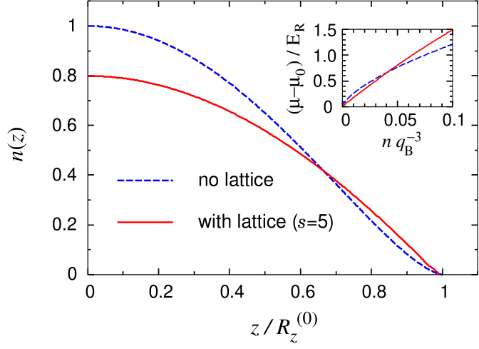
Fig. 1: (Color online) Coarse-grained density profiles of a trapped unitary Fermi gas, $n(r_{\perp}=0,z)$ for $s=0$ and $5$ in units of the central density $n(0)=0.0869q_{\rm B}^{3}$ calculated for $s=0$ (this local density corresponds to $E_{\rm F}/E_{\rm R}=1.88$). The quantity $R_{z}^{(0)}$ is the axial Thomas-Fermi radius for $s=0$. The inset shows the density dependence of the chemical potential of unitary Fermi gases. Here, $\mu_{0}$ is the chemical potential in the limit of $n=0$. This figure is taken from Ref. optlatunit,

3.3. Incompressibility and Effective Mass

The formation of molecules induced by the lattice also has important consequences for $\kappa^{-1}$ and $m^{*}$. Due to the linear density dependence of the chemical potential in the strong lattice region ($\eta_{\rm height}\gg 1$ or $E_{\rm F}/E_{\rm R}\ll s$; or low density limit for a fixed value of $s$), $\kappa^{-1}$ is also proportional to $n$ and $\kappa^{-1}/\kappa^{-1}(s=0)\propto n^{1/3}\rightarrow 0$ for $E_{\rm F}/E_{\rm R}\rightarrow 0$ [see Fig. 2(a)]. This means that the gas becomes highly compressible in the presence of a strong lattice. This is in strong contrast to the ideal Fermi gas corresponding to the BCS limit, which gives nonzero values of $\kappa^{-1}/\kappa^{-1}(s=0)\sim 1$ even in the same limit (see Fig. 2 in Ref. optlatunit, ). On the other hand, in the weak-lattice limit (or high-density limit for a fixed value of $s$), the system reduces to a uniform gas. By using an hydrodynamic theory, which is valid when $E_{\rm F}/E_{\rm R}\gg 1$, and expanding with respect to the small parameter $sE_{\rm R}/E_{\rm F}$, we obtain $\kappa^{-1}$ of unitary Fermi gases in this region as optlatunit

$$\kappa^{-1}\simeq\frac{2}{3}(1+\beta)E_{\rm F}\left[1+\frac{1}{32}(1+\beta)^{-2}\left(\frac{sE_{\rm R}}{E_{\rm F}}\right)^{2}\right]+O\bigl{[}\left(sE_{\rm R}/E_{\rm F}\right)^{4}\bigr{]}.$$ (18)

This is shown by dotted lines in Fig. 2(a). Note that, in this region, $\kappa^{-1}/\kappa^{-1}(s=0)>1$, and it decreases to unity with increasing $E_{\rm F}/E_{\rm R}$. Therefore, $\kappa^{-1}/\kappa^{-1}(s=0)$ should take a maximum value larger than unity in the intermediate region of $E_{\rm F}/E_{\rm R}\sim 1$, as can be seen in Fig. 2(a), which is mainly caused by the bandgap in the longitudinal degree of freedom.

Because the tunneling rate between neighboring sites, which is related to the (inverse) effective mass $1/m^{*}$, is exponentially suppressed with increasing mass, the formation of molecules induced by the lattice can yield a drastic enhancement of $m^{*}$ for $s\gg 1$ in the low-density limit [Fig. 2(b)]. This enhancement makes $m^{*}$ much larger than it is for ideal Fermi gases (see Fig. 2 in Ref. optlatunit ) and for BECs of repulsively-interacting Bose gases (see Fig. 4 in Ref. kramer, ) with the same mass $m$. As $E_{\rm F}/E_{\rm R}$ increases, the effective mass exhibits a maximum at $E_{\rm F}/E_{\rm R}\sim 1$ due to the bandgap in the longitudinal degree of freedom; then, it decreases to the bare mass, $m^{*}=m$. Hydrodynamic theory can explain the behavior of $m^{*}$ of unitary Fermi gases for small $sE_{\rm R}/E_{\rm F}$ optlatunit :

$$\frac{m^{*}}{m}\simeq 1+\frac{9}{32}(1+\beta)^{-2}\left(\frac{sE_{\rm R}}{E_{\rm F}}\right)^{2}+O\bigl{[}\left(sE_{\rm R}/E_{\rm F}\right)^{4}\bigr{]}\ .$$ (19)

The numerical factor in the second term shows that the effect of the lattice is stronger for $m^{*}$ than for $\kappa^{-1}$. It is worth comparing the results with the case of bosonic atoms, where $m^{*}$ decreases monotonically with increasing density because the interaction broadens the condensate wave function and favors the tunneling kramer .

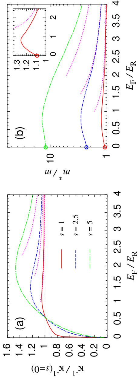
Fig. 2: (Color online) Incompressibility $\kappa^{-1}$ and effective mass $m^{*}$ of unitary Fermi gases for $s=1$ (red), $2.5$ (blue), and $5$ (green). Asymptotic expressions, Eqs. (18) and (19), obtained by using the hydrodynamic theory are shown by the dotted lines. Open circles in panel (b) show $m^{*}$ from Ref. orso, which was obtained by solving the Schrödinger equation for the two-body problem. The $s=1$ results for $m^{*}$ are also shown in the inset on the linear scale. This figure is adapted from Ref. optlatunit, .

In Fig. 3, we show the sound velocity of the unitary Fermi gases in a lattice,

$$c_{\rm s}=\sqrt{\frac{\kappa^{-1}}{m^{*}}}\,,$$ (20)

calculated from the above results for $\kappa^{-1}$ and $m^{*}$. It shows a significant reduction compared to the uniform system, mainly due to the larger effective mass $m^{*}/m>1$ except for the low-density (more precisely, strong lattice) limit in which $\kappa^{-1}$ and, thus, $c_{\rm s}$ show abrupt reductions. Using Eqs. (18) and (19), we obtain the expression of the sound velocity in the weak lattice limit as

$$c_{s}^{2}\simeq{c_{s}^{(0)}}^{2}\left[1-\frac{1}{4}(1+\beta)^{-2}\left(\frac{sE_{\rm R}}{E_{\rm F}}\right)^{2}+O\bigl{[}\left(sE_{\rm R}/E_{\rm F}\right)^{4}\bigr{]}\right]\,,$$ (21)

where $c_{\rm s}^{(0)}\equiv[(2/3)(1+\beta)E_{\rm F}/m]^{1/2}$ is the sound velocity for a uniform system.

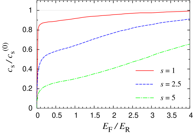
Fig. 3: (Color online) Sound velocity $c_{\rm s}$ of unitary Fermi gases in a lattice in units of the sound velocity $c_{\rm s}^{(0)}=[(2/3)(1+\beta)E_{\rm F}/m]^{1/2}$ for a uniform system. As in Fig. 2, red, blue and green lines correspond to $s=1,2.5$, and $5$, respectively. This figure is taken from Ref. optlatunit,

IV STABILITY

4.1. Landau Criterion

Stability of a superfluid flow is one of the most fundamental issues of superfluidity and was pioneered by Landau landau . He predicted a critical velocity $v_{c}$ of the superflow above which the kinetic energy of the superfluid was large enough to be dissipated by creating excitations (see, e.g., Refs. landau, ; nozieres_pines, ; pethick_smith, ; pitaevskii_stringari, ). This instability is called the Landau or energetic instability, and its critical velocity is the Landau critical velocity.

The celebrated Landau criterion for energetic instability of uniform superfluids is given by landau ; nozieres_pines ; pethick_smith ; pitaevskii_stringari

$$v>v_{c}=\min{\left(\frac{\epsilon(p)}{p}\right)},$$ (22)

where $v$ is the velocity of the superflow, $\epsilon(p)$ is the excitation spectrum in the static case ($v=0$), and $p$ is the magnitude of the momentum $\bm{p}$ of an excitation in the comoving frame of the fluid. Here, $v_{c}$ is determined by the condition for which there starts to exist a momentum $\bm{p}$ at which the excitation spectrum in the comoving frame of a perturber (it can be an obstacle moving in the fluid or a vessel in which the fluid flows) is zero or negative.

For superfluids of weakly interacting Bose gases, the excitation spectrum is given by the Bogoliubov dispersion relation (e.g., Refs. bogoliubov, ; nozieres_pines, ; pethick_smith, ; pitaevskii_stringari, )

$$\epsilon(p)=\sqrt{\frac{p^{2}}{2m}\left(\frac{p^{2}}{2m}+2gn\right)}=c_{s}p\sqrt{1+\left(\frac{p}{2mc_{s}}\right)^{2}}\ ,$$ (23)

with

$$c_{s}=\sqrt{\frac{gn}{m}}$$ (24)

being the sound velocity defined by Eq. (20) [note that $\mu=gn$ and, thus, $\kappa^{-1}=gn$, and $m^{*}=m$ for uniform BECs]. Thus, from Eqs. (22) and (24), the Landau critical velocity is easily seen to be given by the sound velocity $v_{c}=c_{s}$ for $p=0$. This means that, in superfluids of dilute Bose gases, the energetic instability is caused by excitations of long-wavelength phonons. We also note that BECs of non-interacting Bose gases cannot show superfluidity in a sense that $v_{c}=0$ and they cannot support a superflow.

In superfluid Fermi gases, another mechanism can cause the energetic instability: fermionic pair-breaking excitations. In the mean-field BCS theory, the quasiparticle spectrum of uniform superfluid Fermi gases is given by

$$\epsilon(p)=\sqrt{\left(\frac{p^{2}}{2m}-\mu\right)^{2}+\Delta^{2}}\ .$$ (25)

Thus, the Landau critical velocity due to the pair-breaking excitations is given by combescot

$$v_{c}=\sqrt{\frac{1}{m}\left(\sqrt{\mu^{2}+\Delta^{2}}-\mu\right)}\ .$$ (26)

In the deep BCS region, where $\mu\simeq E_{\rm F}\gg\Delta$, we obtain $v_{c}\simeq\Delta/p_{\rm F}$ with $p_{\rm F}\equiv\hbar k_{\rm F}$.

In the BCS-BEC crossover of superfluid Fermi gases, where the above two kinds of excitations exist, the Landau critical velocity is determined by which of them gives smaller $v_{c}$. In the weakly-interacting BCS region ($1/k_{\rm F}a_{s}\lesssim-1$), the pairing gap is exponentially small, $\Delta\sim E_{\rm F}e^{-\pi/2k_{\rm F}|a_{s}|}$, and $v_{c}$ is set by the pair-breaking excitations. On the other hand, in the BEC region ($1/k_{\rm F}a_{s}\gtrsim 1$), where the system consists of weakly-interacting bosonic molecules, creation of long-wavelength superfluid phonon excitations causes an energetic instability. In the unitary region, both mechanisms are suppressed, and the critical velocity shows a maximum value andrenacci ; combescot ; sensarma .

4.2. Stability of Superflow in Lattice Systems

4.2.1. Energetic instability and dynamical instability

For the onset of an energetic instability, energy dissipation is necessary in general; i.e., in closed systems, $v>v_{c}$ is not a sufficient condition for a breakdown of the superflow, so the flow could still persist even at $v>v_{c}$. The energetic instability corresponds to the situation in which the system is located at a saddle point of the energy landscape (i.e., there is at least one direction in which the curvature of the energy landscape is negative).

In the presence of a periodic potential, another type of instability, called dynamical (or modulational) instability, can occur in addition to the energetic instability. The dynamical instability means that small perturbations on a stationary state grow exponentially in the process of (unitary) time evolution without dissipation. Similar to energetically-unstable states, dynamically-unstable states are also located at saddle points in the energy landscape, but a difference from energetically-unstable states is that there are kinematically-allowed excitation processes that satisfy the energy and (quasi-)momentum conservations. This means that an energetic instability is a necessary condition for dynamical instability (see, e.g., Refs. wu2001, and wu2003, for bosons and Ref. ring, for fermions); therefore, the critical value of the (quasi-)momentum for the dynamical instability should always be larger than (or equal to) that for the energetic instability. For such a reason, we shall focus on the energetic instability hereafter note:dynamical .

4.2.2. Determination of the critical velocity

If the energetic instability is caused by long-wavelength superfluid phonon excitations, the critical velocity can be determined by using a hydrodynamic analysis of the excitations machholm03 ; taylor ; pitaevskii05 ; pethick_smith ; vc ; vc_crossover (this should not be confused with the LDA hydrodynamics discussed in Sec. 2.3). This analysis is valid provided that the wavelength of the excitations that trigger the instability is much larger than the typical length scale of the density variation, i.e., the lattice constant $d$.

We consider the continuity equation and the Euler equation for the coarse-grained density $n$ and the coarse-grained (quasi-)momentum $P$ averaged over the length scale larger than the lattice constant:

$$\frac{\partial n}{\partial t}+\bm{\nabla}\cdot\bm{j}= \frac{\partial n}{\partial t}+\frac{\partial}{\partial z}\frac{\partial e}{\partial P}=0,$$ (27)

$$\frac{\partial P}{\partial t}+\frac{\partial\mu}{\partial z}= \frac{\partial P}{\partial t}+\frac{\partial}{\partial z}\frac{\partial e}{\partial n}=0,$$ (28)

where $e=e(n,P)$ is the energy density of the superfluid in the periodic potential for the averaged density $n$ and the averaged (quasi-)momentum $P$. Linearizing with respect to the perturbations of $n(z,t)=n_{0}+\delta n(z,t)$ and $P(z,t)=P_{0}+\delta P(z,t)$ with $\delta n(z,t)$ and $\delta P(z,t)\propto e^{iqz-i\omega t}$, we obtain the dispersion relation of the long-wavelength phonon,

$$\omega(q)=\frac{\partial^{2}e}{\partial n\partial P}q+\sqrt{\frac{\partial^{2}e}{\partial n^{2}}\frac{\partial^{2}e}{\partial P^{2}}}\,|q|\,.$$ (29)

Here, $\hbar\omega$ and $q$ are the energy and the wavenumber of the excitation, respectively. In the first term (so-called Doppler term), $\partial_{n}\partial_{P}e\geq 0$. Thus, the energetic instability occurs when $\omega(q)$ for $q=-|q|$ becomes zero or negative:

$$\frac{\partial^{2}e}{\partial n\partial P}\geq\sqrt{\frac{\partial^{2}e}{\partial n^{2}}\frac{\partial^{2}e}{\partial P^{2}}}\ .$$ (30)

Using this condition, we determine the critical quasi-momentum $P_{c}$ at which the equality of Eq. (30) holds, and finally, we obtain the critical velocity from

$$v_{c}=\frac{1}{n}\left(\frac{\partial e}{\partial P}\right)_{P_{c}}\,.$$ (31)

We note that, for calculating $P_{c}$ and $v_{c}$ using Eqs. (30) and (31), what we only need is the energy density of the stationary states as a function of $n$ and $P$. This can be obtained by solving, e.g., the GP or the BdG equations for the periodic potential.

If the energetic instability of Fermi superfluids is caused by pair-breaking excitations, the critical velocity can be determined by using the quasiparticle energy spectrum $\epsilon_{i}$ obtained from the BdG equations. The energetic instability due to the pair-breaking excitations occurs when some quasiparticle energy $\epsilon_{i}$ becomes zero or negative:

$$\epsilon_{i}\leq 0.$$ (32)

We obtain a critical velocity for the pair-breaking excitations from Eq. (31) evaluated at the critical quasi-momentum determined by this condition.

4.2.3. Critical velocity of superfluid Bose gases and superfluid unitary Fermi gases in a lattice

First, we consider the situation where the LDA is valid; i.e., the lattice constant $d$ is much larger than the healing length $\xi$. This condition corresponds to $gn/E_{\rm R}\gg 1$ for superfluid Bose gases and $E_{\rm F}/E_{\rm R}\gg 1$ for superfluid Fermi gases at unitary (see discussion in Sec. 2.1). In the framework of the LDA hydrodynamics explained in Sec. 2.3, the system is considered to become energetically unstable if there exists some point $z$ at which the local superfluid velocity $v(z)$ is equal to or larger than the local sound velocity $c_{s}(z)$. If the external potential is assumed to have a maximum at $z=z_{0}$ [i.e., $V(z_{0})=V_{0}$ for our periodic potential], then at the same point, the density is minimum, $c_{s}(z)$ is minimum, and $v(z)$ is maximum due to the current conservation; i.e., $j=n(z)v(z)$ being constant. This means that the superfluid first becomes unstable at $z=z_{0}$. Using Eq. (13), we can write the condition for the occurrence of the instability as $m[j_{c}/n_{c}(z_{0})]^{2}=\gamma\mu[n_{c}(z_{0})]=\gamma\alpha n_{c}^{\gamma}(z_{0})$, where $n_{c}(z)$ is the density profile calculated at the critical current kink . By inserting this condition into Eq. (11), we can obtain the following implicit relation for the critical current vc :

$$j_{c}^{2}=\frac{\gamma}{m\alpha^{2/\gamma}}\left[\frac{2\mu_{j_{c}}}{2+\gamma}\left(1-\frac{V(z_{0})}{\mu_{j_{c}}}\right)\right]^{\frac{2}{\gamma}+1}\,.$$ (33)

It is worth noticing that this equation contains only $z$-independent quantities. It is also independent of the shape of the external potential: the only relevant parameter is its maximum value $V(z_{0})$. Moreover, it can be applied to both Bose gases and unitary Fermi gases (see also Refs. mamaladze, ; hakim, ; leboeuf, for bosons).

In Fig. 4, we plot as thick solid red lines the critical velocity in a lattice obtained from the hydrodynamic expression in Eq. (33) for BECs [panel (a)] and unitary Fermi gases [panel (b)]. In both cases, the critical velocity $v_{c}=j_{c}/n_{0}$ ($n_{0}$ is the average density) is normalized to the value of the sound velocity in the uniform gas, $c_{s}^{(0)}$, and is plotted as a function of $V_{0}/\mu_{j=0}$. The limit $V_{0}/\mu_{j=0}\to 0$ corresponds to the usual Landau criterion for a uniform superfluid flow in the presence of a small external perturbation, i.e., a critical velocity equal to the sound velocity of the gas. In this hydrodynamic scheme, as mentioned before, the critical velocity decreases when $V_{0}$ increases mainly because the density has a local depletion and the velocity has a corresponding local maximum, so that the Landau instability occurs earlier. When $V_{0}=\mu_{j_{c}}$, the density exactly vanishes at $z=z_{0}$; hence, the critical velocity goes to zero.

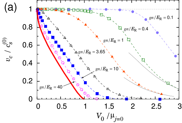
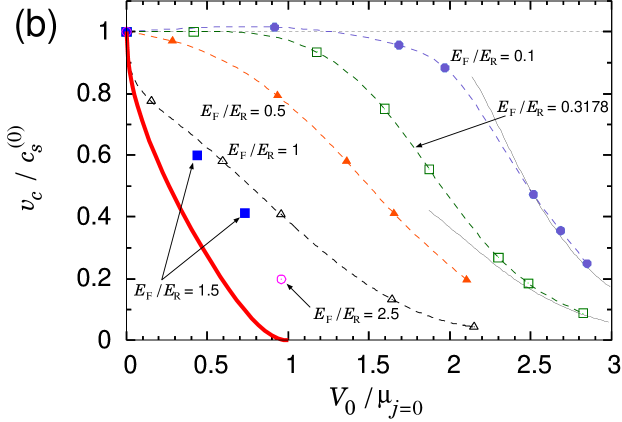
Fig. 4: (Color online) Critical velocity $v_{c}$ for energetic instability of superfluids in a 1D periodic potential. Panel (a) is for superfluids of dilute Bose gases, and panel (b) is for superfluids of dilute Fermi gases at unitarity. The critical velocity is given in units of the sound velocity of a uniform gas, $c_{s}^{(0)}$, and is plotted as a function of the maximum of the external potential in units of the chemical potential $\mu_{j=0}$ of the superfluid at rest. Thick solid lines: prediction of the hydrodynamic theory within the LDA, as calculated from Eq. (33). Symbols: results obtained from the numerical solutions of the GP equation [panel (a)] and the BdG equations [panel (b)]. The thinner black solid lines are the tight-binding prediction, Eq. (35). Dashed lines are guides for the eye. This figure is adapted from Ref. vc, .

Next, we discuss the critical velocity of the energetic instability beyond the LDA vc . Here, we use the energy density $e(n,P)$ of superfluids in a periodic potential calculated by using the mean-field theory in the continuum model, i.e., the GP equation for bosons and the BdG equations for fermions. Based on the energy density, we determine the critical quasi-momentum and the critical velocity from Eqs. (30) and (31).

For Bose superfluids, we plot $v_{c}$ for various values of $gn/E_{\rm R}$ in Fig. 4(a). We can clearly see that these results approach the LDA prediction for $gn/E_{\rm R}\gg 1$, as expected. We also note that $v_{c}$ exhibits a plateau for $gn/E_{\rm R}\lesssim 1$ (i.e., $\xi\gtrsim d$) and small $V_{0}$. This can be understood as follows: If the healing length $\xi$ is larger than the lattice spacing $d$ and $V_{0}/gn$ is not too large, the energy associated with quantum pressure, which is proportional to $1/\xi^{2}$, acts against local deformations of the order parameter, and the latter remains almost unaffected by the modulation of the external potential. This is the region of the plateau in Fig. 4. In terms of Eq. (30), this region occurs when the left-hand side is $\simeq P/m$ and the right-hand side is $\simeq c_{s}^{(0)}$, so that the critical quasi-momentum obeys the relation $P_{c}/m=c_{s}^{(0)}$, which is the usual Landau criterion for a uniform superfluid in the presence of small perturbers. With increasing $V_{0}$, this region ends when $\mu\sim E_{\rm R}$.

If we further increase $V_{0}$, the chemical potential $\mu$ becomes larger than $E_{\rm R}$, the density is forced to oscillate, and $v_{c}/c_{s}^{(0)}$ starts to decrease. The system eventually reaches a region of weakly-coupled superfluids separated by strong barriers, which is well described by the tight-binding approximation (also for $gn/E_{\rm R}\gtrsim 1$, the system enters this region when $V_{0}$ is sufficiently large). There, the energy density is given by a sinusoidal form with respect to $P$ as

$$e(n,P)=e(n,0)+\delta_{J}\left[1-\cos{(\pi P/P_{\rm edge})}\right]\,.$$ (34)

Here, $P_{\rm edge}$ is the quasi-momentum at the edge of the first Brillouin zone; i.e., $P_{\rm edge}=\hbar q_{\rm B}$ for superfluids of bosonic atoms ($P_{\rm edge}=\hbar q_{\rm B}/2$ for those of fermionic atoms). The quantity $\delta_{J}=nP_{\rm edge}^{2}/\pi^{2}m^{*}$ corresponds to the half width of the lowest Bloch band. Because of the sinusoidal shape of the energy density and the large effective mass in the tight-binding limit, the critical quasi-momentum is around $P_{\rm edge}/2$. Thus, we see that, from Eq. (31), the critical velocity is determined by the effective mass as

$$v_{c}\simeq\frac{1}{\pi}\frac{P_{\rm edge}}{m^{*}}\,.$$ (35)

The values of $v_{c}$ obtained from Eq. (35), with $m^{*}$ extracted from the GP calculation of $e(n,P)$, are plotted by thinner black solid lines in Fig. 4(a) for $gn/E_{\rm R}=0.4$ and $1$ in the region of $V_{0}/\mu_{j=0}\gtrsim 2$.

We also calculate the critical velocity by using another method based on a complete linear stability analysis for the GP energy functional as in Refs. wu2001, ; machholm03, , and modugno, (see also Refs. pethick_smith, and wu2003, ). We have checked that the results agree with those obtained from Eq. (30) based on the hydrodynamic analysis to within 1% over the whole range of $gn/E_{\rm R}$ and $V_{0}$ considered in the present work. This confirms that the energetic instability in the periodic potential is triggered by long-wavelength excitations, because the excitation energy of the sound mode is the smallest in this limit.

For superfluid unitary Fermi gases, we plot $v_{c}$ for various values of $E_{\rm F}/E_{\rm R}$ in Fig. 4(b). We observe qualitatively similar results compared to those for bosons plotted in Fig. 4(a). For $E_{\rm F}/E_{\rm R}\lesssim 1$, the critical velocity $v_{c}$ shows a plateau at small $V_{0}$, and it decreases from $\simeq c_{s}^{(0)}$ with increasing $V_{0}$. For larger $E_{\rm F}/E_{\rm R}>1$, $v_{c}$ approaches the LDA result (thick solid red line). In the region of large $V_{0}$ such that $V_{0}/\mu$ is sufficiently large, $v_{c}$ is well described by the tight-binding expression in Eq. (35) plotted by thinner black solid lines in Fig. 4(b). Here, we use $m^{*}$ calculated from the BdG equations. We also note that the pair-breaking excitations are irrelevant to the energetic instability at unitarity except for very low densities such that $E_{\rm F}/E_{\rm R}\ll 1$ and small, but nonzero, $V_{0}$. These excitations are important on the BCS side of the BCS-BEC crossover, as discussed in Sec. 4.2.4.

Finally, we would like to point out that, in the LDA limit, while the quantities discussed in Sec. III approach the value in the uniform system, the critical velocity of the energetic instability is most strongly affected by the lattice. Figure 4 clearly shows that, as we increase the lattice height, the critical velocity decreases from that in the uniform system most rapidly in the LDA limit. The main reason for this opposite tendency is that the critical velocity is determined only around the potential maxima while the quantities discussed in Sec. III are determined by contributions from the whole region of the system.

4.2.4. Along the BCS-BEC crossover

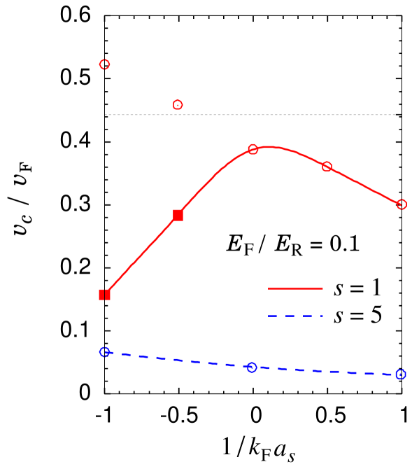
Fig. 5: (Color online) Critical velocity $v_{c}$ of the energetic instability for $E_{\rm F}/E_{\rm R}=0.1$ with $s=1$ and $5$ in the BCS-BEC crossover. Open circles and filled squares show the critical velocity due to long-wavelength phonons and fermionic pair-breaking excitations, respectively. The horizontal dotted line represents the value of the sound velocity $c_{s}^{(0)}$ of a uniform system at unitarity, $c_{s}^{(0)}/v_{\rm F}=(1+\beta)^{1/2}/\sqrt{3}\simeq 0.443$. The red solid line is a guide for the eye.

Here, we extend our discussion on the Landau critical velocity to the BCS-BEC crossover region vc_crossover . As in the uniform systems, both long-wavelength phonon excitations and pair-breaking excitations can be relevant to the energetic instability, depending on the interaction parameter $1/k_{\rm F}a_{s}$. However, there is an additional effect due to the lattice: when the lattice height is much larger than the Fermi energy, the periodic potential can cause pairs of atoms to be strongly bound even in the BCS region, so the pair-breaking excitations are suppressed vc_crossover .

In Fig. 5, we plot $v_{c}$ for superfluid Fermi gases in the BCS-BEC crossover for different values of the lattice height with $s=1$ and $5$. Here, we set $E_{\rm F}/E_{\rm R}=0.1$ as an example. The open circles show $v_{c}$ of the energetic instability caused by long-wavelength superfluid phonon excitations, and the filled squares show that caused by pair-breaking excitations. For a moderate lattice strength of $s=1$, the result for $v_{c}$ is qualitatively the same as that of the uniform system. On the BCS side, the smallest $v_{c}$ is given by the pair-breaking excitations while, on the BEC side, $v_{c}$ is set by the long-wavelength phonon excitations, and around unitarity $v_{c}$ shows a maximum. For a larger value of $s=5$, however, the result is very different from the uniform case. Due to the lattice-induced binding, pair breaking is suppressed so that it does not cause an energetic instability even on the BCS side. (Note that there is no filled square for $s=5$. This means that we do not have a negative quasiparticle energy for any value of $P$ in the whole Brillouin zone. This point will be discussed later.) Throughout the calculated region of $-1\leq 1/k_{\rm F}a_{s}\leq 1$, $v_{c}$ is determined only by the long-wavelength phonon excitations, and $v_{c}$ decreases monotonically with increasing $1/k_{\rm F}a_{s}$.

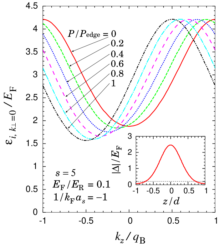
Fig. 6: (Color online) Lowest band of the quasiparticle energy spectrum $\epsilon_{i}$ for large lattice height with $s=5$ and $E_{\rm F}/E_{\rm R}=0.1$ (i.e., $E_{\rm F}/V_{0}=0.02$) in the BCS region at $1/k_{\rm F}a_{s}=-1$. Here, we show the first radial branch with $k_{\perp}^{2}\equiv k_{x}^{2}+k_{y}^{2}=0$, which always gives the smallest values of $\epsilon_{i}$ in this case. The inset shows the amplitude $|\Delta(z)|$ of the order parameter at $P=0$. The horizontal dotted line shows the amplitude of the order parameter for a uniform system at the same value of $1/k_{\rm F}a_{s}=-1$. This figure is adapted from Ref. vc_crossover, .

The effect of the lattice-induced molecular formation can be clearly seen in the quasiparticle energy spectrum $\epsilon_{i}$ and in the enhancement of the order parameter $\Delta(z)$. In Fig. 6, we show $\epsilon_{i}$ and $|\Delta(z)|$ in the case of $s=5$, $E_{\rm F}/E_{\rm R}=0.1$, and $1/k_{\rm F}a_{s}=-1$. The spectrum for $P=0$ shows a quadratic dependence on $k_{z}$ with a positive curvature around $k_{z}=0$, and there are no minima at $k_{z}\neq 0$. Even though the figure represents a case in the BCS region, the structure of $\epsilon_{i}$ is consistent with the formation of bound pairs. We can also see that the spectrum never becomes negative for any values of $P$ in the first Brillouin zone. In the inset of the same figure, we show the amplitude $|\Delta(z)|$ of the order parameter at $P=0$. Here, we see a large enhancement of $|\Delta(z)|$ near $z=0$ compared to the uniform system, which shows the formation of bosonic bound molecules. We also note that the minimum value of $|\Delta(z)|$ at $z/d=\pm 1$ is smaller than, but still comparable to, the value of $|\Delta|$ in the uniform case, suggesting that the system is, indeed, in the superfluid phase.

4.2.5. Experiments

In closing this section, we briefly summarize experimental studies on the stability of a superfluid. Using cold atomic gases, stability of the superfluid and its critical velocity was first experimentally studied in Ref. raman, and further examined in Ref. onofrio, . These experiments used a large (diameter $\gg\xi$) and strong (height $\gg\mu$) vibrating circular potential in a BEC. However, it has been concluded that what was observed in these works was not likely to be the energetic instability: dynamical nucleation of vortices by vibrating potential onofrio . Recently, Ramanathan et al. performed a new experiment on the stability of a superflow with a different setup ramanathan . They used a BEC flowing in a toroidal trap with a tunable weak link (width of the barrier along the flow direction much larger than $\xi$). In that experiment, they obtained a critical velocity consistent with the energetic instability due to vortex excitations feynman . For 2D Bose gases, the stability of the superfluidity and the critical velocity were also studied recently desbuquois .

Regarding the superflow in optical lattices, its stability was first experimentally studied in Ref. burger, . In that experiment, they used a cigar-shaped BEC that underwent a center-of-mass oscillation in a harmonic trap in the presence of a weak 1D optical lattice, and they measured the critical velocity. Although their original conclusion was that they had measured the Landau critical velocity for the energetic instability, further careful experimental desarlo and theoretical wu2001 ; modugno follow-up studies clarified that the instability observed in Ref. burger, was a dynamical instability. In this follow-up experiment by De Sarlo et al. desarlo , they employed an improved setup, i.e., a 1D optical lattice moving at constant and tunable velocities instead of an oscillating BEC in a static lattice. With this new setup, they succeeded in observing both energetic desarlo and dynamical desarlo ; fallani instabilities, and obtained a very good agreement with theoretical predictions desarlo ; modugno ; fallani . It is worthwhile to stress that this understanding was finally obtained through a continuous effort over a few years by the same group.

Experimental study on the stability of superfluid Fermi gases in optical lattices was carried out by Miller et al. miller . Similar to the experiment of Ref. desarlo, , they also used a 1D lattice moving at constant and tunable velocities. A different point is that, instead of imposing a periodic potential on the whole cloud, they produced a lattice potential only in the central region of the cloud. They measured the critical velocity of the energetic instability in the BCS-BEC crossover and found that it was largest around unitarity. They also did a systematical measurement of the critical velocity at unitarity for various lattice heights. However, there is a significant discrepancy from a theoretical prediction vc , so further studies are needed.

V ENERGY BAND STRUCTURE

In this section, we discuss how the superfluidity can affect the energy band structures of ultracold atomic gases in periodic optical potentials. Starting with the noninteracting particles in a periodic potential, we obtain the well-known sinusoidal energy band structure. When the interparticle interaction is turned on in such a way that the superfluidity appears, we see a drastic change in the energy band structure. For BECs, it has been pointed out that the interaction can change the Bloch band structure, causing the appearance of a loop structure called “swallowtail” in the energy dispersion wu_st ; diakonov ; seaman ; danshita . This is due to the competition between the external periodic potential and the nonlinear mean-field interaction: the former favors a sinusoidal band structure while the latter tends to make the density smoother and the energy dispersion quadratic. When the nonlinearity wins, the effect of the external potential is screened, and a swallowtail energy loop appears mueller . This nonlinear effect requires the existence of an order parameter; consequently, the emergence of swallowtails can be viewed as a peculiar manifestation of superfluidity in periodic potentials.

Qualitatively, one can argue in a similar way on the existence of the swallowtail energy band structure in Fermi superfluids in optical lattices; the competition between the external periodic potential energy and the nonlinear interaction energy ($g|\sum_{i}u_{i}(\mathbf{r})v_{i}^{*}(\mathbf{r})|^{2}$) determines the energy band structure. However, the interaction energy in the Fermi gas is more involved, and the unified view along the crossover from the BCS to the BEC states is a nontrivial and interesting problem in itself. To answer the questions of 1) whether or not swallowtails exist in Fermi superfluids and 2) whether unique features that are different from those in bosons exist, we solve the BdG equations [see Eq. (9)] of a two-component unpolarized dilute Fermi gas subject to a one-dimensional (1D) optical lattice swallowtail .

5.1. Swallowtail Energy Spectrum

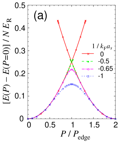
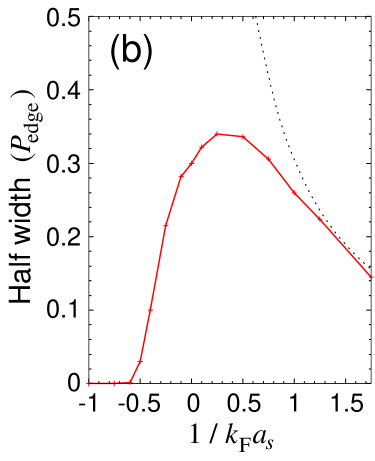
Fig. 7: (Color online) (a) Energy $E$ per particle as a function of the quasi-momentum $P$ for various values of $1/k_{\rm F}a_{s}$, and (b) half width of the swallowtails along the BCS-BEC crossover. These results are obtained for $s=0.1$ and $E_{\rm F}/E_{\rm R}=2.5$. The quasi-momentum $P_{\rm edge}=\hbar q_{\rm B}/2$ fixes the edge of the first Brillouin zone. The dotted line in (b) is the half width in a BEC obtained by solving the GP equation; it vanishes at $1/k_{\rm F}a_{s}\simeq 10.6$. This figure is taken from Ref. swallowtail, .

The energy per particle in the lowest Bloch band as a function of the quasi-momentum $P$ for various values of $1/k_{\rm F}a_{s}$ is computed footnote_parameter_value . The results in Fig. 7(a) show that the swallowtails appear above a critical value of $1/k_{\rm F}a_{s}$ where the interaction energy is strong enough to dominate the lattice potential. In Fig. 7(b), the half-width of the swallowtails from the BCS to the BEC side is shown. It reaches a maximum near unitarity ($1/k_{\rm F}a_{s}=0$). In the far BCS and BEC limits, the width vanishes because the system is very weakly interacting and the band structure tends to be sinusoidal. When approaching unitarity from either side, the interaction energy increases and can dominate over the periodic potential, which means that the system behaves more like a translationally-invariant superfluid and the band structure follows a quadratic dispersion terminating at a maximum $P$ larger than $P_{\rm edge}$.

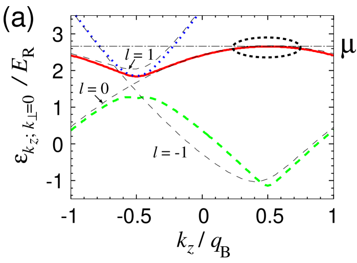
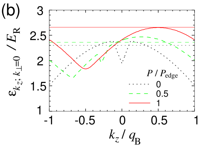
Fig. 8: (Color online) (a) Lowest three Bloch bands of the quasiparticle energy spectrum at $k_{\perp}=0$ for $P=P_{\rm{edge}}$ and $1/k_{\rm F}a_{s}=-0.62$. Thin black dashed lines labeled by $l$’s show the approximate energy bands obtained from Eq. (36) by using $\mu\simeq 2.66E_{\rm R}$ and $|\Delta|\simeq|\Delta(0)|\simeq 0.54E_{\rm R}$. (b) Bloch band of the quasiparticle energy spectrum around the chemical potential for $P/P_{\rm{edge}}=0$ (black dotted), $0.5$ (green dashed), and $1$ (red solid) at $k_{\perp}=0$ and $1/k_{\rm F}a_{s}=-0.62$ in the case of $s=0.1$ and $E_{\rm F}/E_{\rm R}=2.5$. Each horizontal line denotes the value of the chemical potential for the corresponding value of $P$. This figure is adapted from Ref. swallowtail, .

The emergence of swallowtails on the BCS side for $E_{\rm F}/E_{\rm R}\gtrsim 1$ is associated with peculiar structures of the quasiparticle energy spectrum around the chemical potential. In the presence of a superflow moving in the $z$ direction with wavevector $Q$ ($\equiv P/\hbar$), the quasiparticle energies are given by the eigenvalues in Eq. (9). Because the potential is shallow ($s\ll 1$), some qualitative results can be obtained even when ignoring $V_{\text{ext}}(z)$ except for its periodicity. With this assumption, we obtain

$$\epsilon_{\mathbf{k}}\!\approx\!\frac{(k_{z}\!+\!2q_{\rm B}l)Q}{m}\!+\!\sqrt{\left[\!\frac{k_{\perp}^{2}\!+\!(k_{z}\!+\!2q_{\rm B}l)^{2}\!+\!Q^{2}}{2m}\!-\!\mu\right]^{2}\!\!\!+\!|\Delta|^{2}}\ ,$$ (36)

with $l$ being integers for the band index. If $Q=0$, the $l=0$ band has the energy spectrum $\sqrt{[(k_{\perp}^{2}+k_{z}^{2})/2m-\mu]^{2}+|\Delta|^{2}}$, which has a local maximum at $k_{z}=k_{\perp}=0$. When $Q=P_{\rm edge}/\hbar$, the spectrum is tilted, and the local maximum moves to $k_{z}\simeq q_{\rm B}/2$ provided $|\Delta|\ll E_{\rm F}$ (and $E_{\rm F}/E_{\rm R}\gtrsim 1$). In the absence of the swallowtail, the full BdG calculation, indeed, gives a local maximum at $k_{z}=q_{\rm B}/2$, and the quasiparticle spectrum is symmetric about this point, which reflects that the current is zero. As $E_{\rm F}/E_{\rm R}$ increases, the band becomes flatter as a function of $k_{z}$ and narrower in energy.

In Fig. 8(a), we show the quasiparticle energy spectrum at $k_{\perp}=0$ for $P=P_{\rm{edge}}$. When the swallowtail is on the edge of appearing, the top of the narrow band just touches the chemical potential $\mu$ [see the dotted ellipse in Fig. 8(a)]. Suppose $1/k_{\rm F}a_{s}$ is slightly larger than the critical value so that the top of the band is slightly above $\mu$. In this situation, a small change in the quasi-momentum $P$ causes a change of $\mu$. In fact, when $P$ is increased from $P=P_{\rm{edge}}$ to larger values, the band is tilted, and the top of the band moves upwards; the chemical potential $\mu$ should also increase to compensate for the loss of states available, as shown in Fig. 8(b). This implies ${\partial}\mu/{\partial}P>0$. On the other hand, because the system is periodic, the existence of a branch of stationary states with ${\partial}\mu/{\partial}P>0$ at $P=P_{\rm{edge}}$ implies the existence of another symmetric branch with ${\partial}\mu/{\partial}P<0$ at the same point, thus suggesting the occurrence of a swallowtail structure.

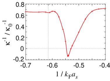
Fig. 9: Incompressibility $\kappa^{-1}$ at $P=P_{\rm{edge}}$ around the critical value of $1/k_{\rm F}a_{s}\approx-0.62$ where the swallowtail starts to appear. The quantity $\kappa_{0}^{-1}$ is the incompressibility of the homogeneous free Fermi gas of the same average density. In both panels, we have used the values $s=0.1$ and $E_{\rm F}/E_{\rm R}=2.5$. This figure is adapted from Ref. swallowtail, .

5.2. Incompressibility

A direct consequence of the existence of a narrow band in the quasiparticle spectrum near the chemical potential is a strong reduction of the incompressibility $\kappa^{-1}=n{\partial}\mu(n)/{\partial}n$ close to the critical value of $1/k_{\rm F}a_{s}$ in the region where swallowtails start to appear in the BCS side (see Fig. 9). A dip in $\kappa^{-1}$ occurs in the situation where the top of the narrow band is just above $\mu$ for $P=P_{\rm edge}$ ($1/k_{\rm F}a_{s}$ is slightly above the critical value). An increase in the density $n$ has little effect on $\mu$ in this case because the density of states is large in this range of energy and the new particles can easily adjust themselves near the top of the band by a small increase of $\mu$. This implies that ${\partial}\mu(n)/{\partial}n$ is small and that the incompressibility has a pronounced dip note_incompress . It is worth noting that on the BEC side, the appearance of the swallowtail is not associated with any significant change in the incompressibility. In fact, for a Bose gas with an average density $n_{b0}$ of bosons, the exact solution of the GP equation gives $\kappa^{-1}=n_{b0}g$ near the critical conditions for the occurrence of swallowtails, being a smooth and monotonic function of the interaction strength.

5.3. Profiles of Density and Pairing Fields

Both the pairing field and the density exhibit interesting features in the range of parameters where the swallowtails appear. This is particularly evident at the Brillouin zone boundary, $P=P_{\rm{edge}}$. The full profiles of $|\Delta(z)|$ and $n(z)$ along the lattice vector ($z$ direction) are shown in Fig. 10. In general, $n(z)$ and $|\Delta(z)|$ take maximum (minimum) values where the external potential takes its minimum (maximum) values. By increasing the interaction parameter $1/k_{\rm F}a_{s}$, we find that the order parameter $|\Delta|$ at the maximum ($z=\pm d/2$) of the lattice potential exhibits a transition from zero to nonzero values at the critical value of $1/k_{\rm F}a_{s}$ at which the swallowtail appears. Note that here we plot the absolute value of $\Delta$; the order parameter $\Delta$ behaves smoothly and changes sign.

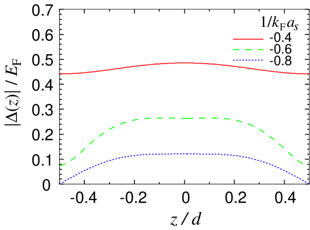
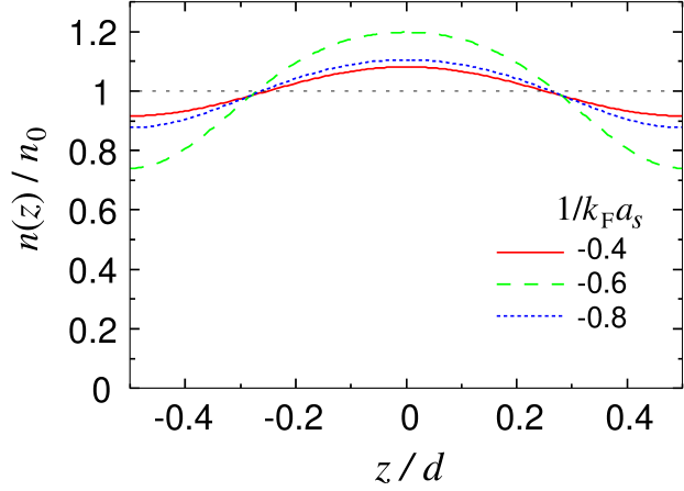
Fig. 10: Profiles of the pairing field $|\Delta(z)|$ and the density $n(z)$ at $1/k_{\rm F}a_{s}=-0.8$ (blue dotted), $-0.6$ (green dashed), and $-0.4$ (red solid) for $P=P_{\rm{edge}}$ in the case of $s=0.1$ and $E_{\rm F}/E_{\rm R}=2.5$. The swallowtail starts to appear at a critical value of $1/k_{\rm F}a_{s}\approx-0.62$. This figure is taken from Ref. swallowtail, .

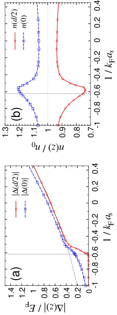
Fig. 11: (Color online) Profiles of (a) the pairing field $|\Delta(z)|$ and (b) the density $n(z)$ for changing $1/k_{\rm F}a_{s}$ for $P=P_{\rm{edge}}$ in the case of $s=0.1$ and $E_{\rm F}/E_{\rm R}=2.5$. The values of $|\Delta(z)|$ and $n(z)$ at the minimum ($z=0$, blue $\square$) and at the maximum ($z=\pm d/2$, red $\times$) of the lattice potential are shown. The vertical dotted lines show the critical value of $1/k_{\rm F}a_{s}$ above which the swallowtail exists. The dotted curve in (a) shows $|\Delta|$ in a uniform system. This figure is taken from Ref. swallowtail, .

In Fig. 11, we show the magnitude of the pairing field $|\Delta(z)|$ and the density $n(z)$ calculated at the minimum ($z=0$) and at the maximum ($z=\pm d/2$) of the lattice potential. The figure shows that $|\Delta(d/2)|$ remains zero in the BCS region until the swallowtail appears at $1/k_{\rm F}a_{s}\approx-0.62$. Then, it increases abruptly to values comparable to $|\Delta(0)|$, which means that the pairing field becomes almost uniform at $P=P_{\rm{edge}}$ in the presence of swallowtails. As regards the density, we find that the amplitude of the density variation, $n(0)-n(d/2)$, exhibits a pronounced maximum near the critical value of $1/k_{\rm F}a_{s}$.

In contrast, on the BEC side, the order parameter and the density are smooth monotonic functions of the interaction strength even in the region where the swallowtail appears. At $P=P_{\rm{edge}}$, the solution of the GP equation for bosonic dimers gives the densities $n_{b}(0)=n_{b0}(1+V_{0}/2n_{b0}g_{b})$ and $n_{b}(d/2)=n_{b0}(1-V_{0}/2n_{b0}g_{b})$, with $V_{0}/2n_{b0}g_{b}=(3\pi/4)(sE_{\rm R}/E_{\rm F})(1/k_{\rm F}a_{s})$, where $g_{b}\equiv 4\pi\hbar^{2}a_{b}/m_{b}$, and $a_{b}$ and $m_{b}$ are the scattering length and the mass of bosonic dimers, respectively wu_st ; bronski ; note-nb . Near the critical value of $1/k_{\rm F}a_{s}$, unlike the BCS side, the nonuniformity just decreases all the way even after the swallowtail appears. The local density at $z=d/2$ is zero until the swallowtail appears on the BEC side while it is nonzero on the BCS side irrespective of the existence of the swallowtail. The qualitative behavior of $|\Delta(z)|$ around the critical point of $1/k_{\rm F}a_{s}$ is similar to that of $n_{b}(z)$ because $n_{b}(\mathbf{r})=(m^{2}a_{s}/8\pi)|\Delta(\mathbf{r})|^{2}$ bdgtogp in the BEC limit.

VI QUANTUM PHASES OF COLD ATOMIC GASES IN OPTICAL LATTICES

So far, we have discussed some superfluid features of cold atomic gases in an optical lattice by mainly focusing on our works. In this section, we discuss some important topics regarding various quantum phases that the cold atomic gases on optical lattices can show/simulate. In this section, strong enough periodic potentials to ignore the next-nearest hopping and small average numbers of particles per lattice site will be assumed so that the system can be described by the Hubbard lattice model.

6.1. Quantum Phase Transition from a Superfluid to a Mott Insulator

At a temperature of absolute zero, cold atomic gases in optical lattices can undergo a quantum phase transition from superfluid to Mott insulator phases as the interaction strength between atoms is tuned from the weakly- to the strongly-interacting region Jaksch . The quantum phase transition of an interacting boson gas in a periodic lattice potential can be captured by the following Bose-Hubbard Hamiltonian:

$$H=-J\sum_{\langle i,j\rangle}(\hat{b}_{i}^{\dagger}\hat{b}_{j}+\text{h.c.})+\frac{U}{2}\sum_{i}\hat{n}_{i}(\hat{n}_{i}-1)\,,$$

where $\hat{b}_{i}$ and $\hat{b}_{i}^{\dagger}$ are annihilation and creation operators of a bosonic atom on the $i$-th lattice site and $\hat{n}_{i}=\hat{b}_{i}^{\dagger}\hat{b}_{i}$ is the atomic number operator on the $i$-th site. The first term is the kinetic energy term whose strength is characterized by the hopping matrix element $J$ between adjacent sites $\langle i,j\rangle$, and $U(>0)$ in the second term is the strength of a short-range repulsive interactions between bosonic atoms.

In the limit where the kinetic energy dominates, the many-body ground state of $N$ atoms and $M$ lattice sites is a superposition of delocalized Bloch states with lowest energy (quasi-momentum ${\mathbf{k}}=0$):

$$|\Psi_{\text{SF}}\rangle_{U/J=0}\propto(\hat{b}_{{\mathbf{k}}=0}^{\dagger})^{N}|0\rangle\propto\left(\sum_{i=1}^{M}\hat{b}_{i}^{\dagger}\right)^{N}|0\rangle\,,$$ (37)

where $|0\rangle$ is the empty lattice. This state has perfect phase correlation between atoms on different sites while the number of atoms on each site is not fixed. This superfluid phase has gapless phonon excitations.

In the limit where the interactions dominate (so-called, “atomic limit”), the fluctuations in the local atom number become energetically unfavorable, and the ground state is made up of localized atomic wavefunctions with a fixed number of atoms per lattice site. The many-body ground state with a commensurate filling of $n$ atoms per lattice site is given by

$$|\Psi_{\text{MI}}\rangle_{J/U=0}\propto\prod_{i=1}^{M}(\hat{b}_{i}^{\dagger})^{n}|0\rangle\,.$$ (38)

There is no phase correlation between different sites because the energy is independent of the phases of the wavefunctions on each site. This Mott insulator state, unlike the superfluid state, cannot be described by using a macroscopic wavefunction. The lowest excited state can be obtained by moving one atom from one site to another, which gives an energy gap of $\Delta=(U/2)[(n+1)^{2}+(n-1)^{2}-2n^{2}]=U$.

As the ratio of the interaction term to the tunneling term increases ($U/J$ can be controlled by changing the depth $V_{0}$ of the optical lattice even without using the Feshbach resonances), the system will undergo a quantum phase transition from a superfluid state to a Mott insulator state accompanying the opening of the energy gap in the excitation spectrum. Greiner et al. realized experimentally a quantum phase transition from a Bose-Einstein condensate of ${}^{87}\text{Rb}$ atoms with weak repulsive interactions to a Mott insulator in a three-dimensional optical lattice potential Greiner_SF_Mott . Notably, they could induce reversible changes between these two ground states by changing the strength $V_{0}$ of the optical lattice. The superfluid-to-Mott-insulator transitions were also achieved in one- and two-dimensional cold atomic Bose gases Mott_dim . The Mott insulator phases of atomic Fermi gases with repulsive interactions on a three-dimensional optical lattice have been realized, and the entrance into the Mott insulating states was observed by verifying vanishing compressibility and by measuring the suppression of doubly-occupied sites Jordens_Mott ; Schneider_Mott .

6.2. Quantum Phase Transition from a Paramagnet to an Antiferromagnet

Sachdev et al. showed that the one-dimensional Mott insulator of spinless bosons in a tilted optical lattice can be mapped onto a quantum Ising chain Sachdev2002 . The Bose-Hubbard Hamiltonian for a tilted optical lattice takes the form

$$H=-J\sum_{i}(\hat{b}_{i}\hat{b}_{i+1}^{\dagger}+\hat{b}_{i}^{\dagger}\hat{b}_{i+1})+\frac{U}{2}\sum_{i}\hat{n}_{i}(\hat{n}_{i}-1)-E\sum_{i}i\hat{n}_{i}\ ,$$

where $E$ is the lattice potential gradient per lattice spacing. For a tilt near $E=U$, the energy cost of moving an atom to its neighbor (from site $i$ to site $i+1$) is zero. If we start with a Mott insulator with a single atom per site, an atom can resonantly tunnel into the neighboring site to produce a dipole state (at the link) consisting of a quasihole-quasiparticle pair on nearest neighbor sites. Only one dipole can be created per link, and neighboring links cannot support dipoles together. This nearest-neighbor constraint is the source of the effective dipole-dipole interaction that results in a density wave ordering. If a dipole creation operator $\hat{d}_{i}^{\dagger}=\hat{b}_{i}\hat{b}_{i+1}^{\dagger}/\sqrt{2}$ is defined, the Bose-Hubbard Hamiltonian is mapped onto the dipole Hamiltonian:

$$H=-\sqrt{2}J\sum_{i}(\hat{d}_{i}^{\dagger}+\hat{d}_{i})+(U-E)\sum_{i}\hat{d}_{i}^{\dagger}\hat{d}_{i},$$

with the constraint $\hat{d}_{i}^{\dagger}\hat{d}_{i}\leq 1$ and $\hat{d}_{i}^{\dagger}\hat{d}_{i}\hat{d}_{i+1}^{\dagger}\hat{d}_{i+1}=0$. If the dipole present/absent link is identified with a pseudospin up/down, $\hat{S}_{i}^{z}=\hat{d}_{i}^{\dagger}\hat{d}_{i}-1/2$, the pseudospin-1/2 Hamiltonian takes the form of a quantum Ising chain:

$$H = J_{S}\sum_{i}\hat{S}_{i}^{z}\hat{S}_{i+1}^{z}-2\sqrt{2}J\sum_{i}\hat{S}_{i}^{x}+(J_{S}-D)\sum_{i}\hat{S}_{i}^{z}$$

$$= J_{S}\sum_{i}(\hat{S}_{i}^{z}\hat{S}_{i+1}^{z}-h_{x}\hat{S}_{i}^{x}+h_{z}\hat{S}_{i}^{z})\,,$$

where $D=E-U$ and $\sum_{i}J_{S}(\hat{S}_{i}^{z}+1/2)(\hat{S}_{i+1}^{z}+1/2)$, with $J_{S}\to\infty$ being added to the Hamiltonian for implementing the constraint $\hat{d}_{i}^{\dagger}\hat{d}_{i}\hat{d}_{i+1}^{\dagger}\hat{d}_{i+1}=0$. The dimensionless transverse and longitudinal fields are defined as $h_{x}=2^{3/2}J/J_{S}$ and $h_{z}=1-D/J_{S}$, respectively.

Thus, a quantum phase transition from a paramagnetic phase ($D\lesssim 0$) to an antiferromagnetic phase ($D\gtrsim 0$) can be studied by changing the lattice potential gradient $E$ between adjacent sites. With ${}^{87}\text{Rb}$ atoms, a quantum simulation of antiferromagnetic spin chains in an optical lattice was done, and a phase transition to the antiferromagnetic phase from the paramagnetic phase was observed Ising_chain .

VII SUMMARY AND OUTLOOK

In this article, we have focused on some superfluid properties of cold atomic gases in an optical lattice periodic along one spatial direction: basic macroscopic and static properties, the stability of the superflow, and peculiar energy band structures. As a complement, some phases other than the superfluid phase have been discussed in the last section. Considering the rapid growth and interdisciplinary nature of the research on cold atomic gases in optical lattices, it is practically impossible to cover all perspectives. We conclude by mentioning a few of them.

The high controllability of the lattice potential opens many possibilities: An optical disordered lattice can be constructed to study the problem of the Anderson localization of matter waves and the resulting phases disorder . The time modulation of the optical lattice is shown to tune the magnitude and the sign of the tunnel coupling in the Hubbard model, which allows us to study various phases time_modulation . Cold atomic gases in optical lattices may uncover many exotic phases that are still under debate or even lack solid state analogs.

Due to their long characteristic time scales and large characteristic length scales, cold atomic gases are good playgrounds for the experimental observation and control of their dynamics. Particularly, a sudden quench can be realized experimentally. The nonequilibrium dynamics after sudden quenches can be studied with high precision in experiments to discriminate between candidate theories. Long-standing problems such as thermalization, its connection with non-integrability and/or quantum chaos are actively sought-after topics in this direction non-equilibrium .

The charge neutrality of atoms seems to limit the use of this system as a quantum simulator. However, the internal states of an atom, together with atom-laser interactions, can be exploited for the atom to gain geometric Berry’s phases, which amounts to generating artificial gauge fields interacting with these charge-neutral particles artificial_gauge . In this way, interactions with electromagnetic fields, spin-orbit coupling, and even non-Abelian gauge fields can be emulated to open the door to the study of the physics of the quantum Hall effects, topological superconductors/insulators, and high energy physics by using cold atoms in the future.

Cold atomic gases provide a promising platform for controlling dissipation and for engineering the Hamiltonian, e.g., by controlling the coupling with a subsystem acting as a reservoir, by using external fields that induce losses of trapped atoms, etc. This possibility will allow us to use the cold atomic gases as quantum simulators of open systems. In addition, the controlled dissipation will offer an opportunity to study the quantum dynamics driven by dissipation and its steady states, and to study the non-equilibrium phase transitions among the steady states determined by the competition between the coherent and the dissipative dynamics. Furthermore, controlling the dissipation will pave the way to the design of Liovillian and to the dissipation-driven state-preparation (e.g., Ref. dissipation, ).

Last, but not least, cold atomic gases in optical lattices are also useful for the precision measurements; the “optical lattice clock” consists of millions of atomic clocks trapped in an optical lattice and working in parallel. The large number of simultaneously-interrogated atoms greatly improves the stability of the clock, and state-of-the-art optical lattice clocks outperform the primary frequency standard of Cs clocks (Ref. optlatclock, and references therein). Bloch oscillations of cold atomic gases in optical lattices offer a promising way of measuring forces at a spatial resolution of few micrometers (e.g., Ref. bloch_osc, ). Precision measurement devices/techniques will enable high-precision tests of time and space variations of the fundamental constants, the weak equivalence principle, and Newton’s gravitational law at short distances.

- (1) M. H. Anderson, J. R. Ensher, M. R. Matthews, C. E. Wieman, and E. A. Cornell, Science 269, 198 (1995); C. C. Bradley, C. A. Sackett, J. J. Tollett, and R. G. Hulet, Phys. Rev. Lett. 75, 1687 (1995); K. B. Davis, M-O. Mewes, M. R. Andrews, N. J. Van Druten, D. S. Durfee, D. M. Kurn, and W. Ketterle, Phys. Rev. Lett. 75, 3969 (1995).
- (2) M. W. Zwierlein, J. R. Abo-Shaeer, A. Schirotzek, C. H. Schunck, and W. Ketterle, Nature 435, 1047 (2005).
- (3) A. J. Leggett, Rev. Mod. Phys. 73, 307 (2001).
- (4) F. Dalfovo, S. Giorgini, L. P. Pitaevskii, and S. Stringari, Rev. Mod. Phys. 71, 463 (1999).
- (5) I. Bloch, J. Dalibard, and W. Zwerger, Rev. Mod. Phys. 80, 885 (2008).
- (6) S. Giorgini, L. P. Pitaevskii, and S. Stringari, Rev. Mod. Phys. 80, 1215 (2008).
- (7) I. Bloch, J. Dalibard, and S. Nascimbène, Nature Phys. 8, 267 (2012).
- (8) U. Fano, Phys. Rev. 124, 1866 (1961); H. Feshbach, Ann. Phys. (N.Y.) 19, 287 (1962).
- (9) D. M. Eagles, Phys. Rev. 186, 456 (1969); A. J. Leggett, in Modern Trends in the Theory of Condensed Matter (Springer-Verlag, Berlin, 1980), pp. 13-27; P. Nozières, and S. Schmitt-Rink, J. Low Temp. Phys. 59, 195 (1985); C. A. R. Sá de Melo, M. Randeria, and J. R. Engelbrecht, Phys. Rev. Lett. 71, 3202 (1993).
- (10) P. Fulde and R. A. Ferrell, Phys. Rev. 135, A550 (1964); A. I. Larkin and Y. N. Ovchinnikov, Sov. Phys. JETP 20, 762 (1965).
- (11) G. B. Partridge, W. Li, R. I. Kamar, Y. A. Liao, and R. G. Hulet, Science 311, 503 (2006); M. W. Zwierlein, C. H. Schunck, A. Schirotzek, and W. Ketterle, Nature 442, 54 (2006); Y. Shin, C. H. Schunck, A. Schirotzek, and W. Ketterle, Nature 451, 689 (2008).
- (12) C. Cao, E. Elliott, J. Joseph, H. Wu, J. Petricka, T. Schafer, and J. E. Thomas, Science 331, 58 (2011); B. V. Jacak and B. Muller, Science 337, 310 (2012).
- (13) O. Morsch and M. Oberthaler, Rev. Mod. Phys. 78, 179 (2006).
- (14) V. I. Yukalov, Laser Phys. 19, 1 (2009).
- (15) W. S. Bakr, A. Peng, M. E. Tai, R. Ma, J. Simon, J. I. Gillen, S. Fölling, L. Pollet, and M. Greiner, Science 329, 547 (2010); C. Weitenberg, M. Endres, J. F. Sherson, M. Cheneau, P. Schauß, T. Fukuhara, I. Bloch, and S. Kuhr, Nature 471, 319 (2011).
- (16) Q. Niu, X. G. Zhao, G. A. Georgakis, and M. G. Raizen, Phys. Rev. Lett. 76, 4504 (1996); M. Ben Dahan, E. Peik, J. Reichel, Y. Castin, and C. Salomon, Phys. Rev. Lett. 76, 4508 (1996); B. P. Anderson and M. A. Kasevich, Science 282, 1686 (1998).
- (17) M. Greiner, O. Mandel, T. Esslinger, T. W. Hänsch, and I. Bloch, Nature 415, 39 (2002).
- (18) A. Derevianko and H. Katori, Rev. Mod. Phys. 83, 331 (2011).
- (19) D. Jaksch and P. Zoller, Ann. Phys. (N.Y.) 315, 52 (2005).
- (20) G. Watanabe and T. Maruyama, in Neutron Star Crust, edited by C. A. Bertulani and J. Piekarewicz (Nova, New York, 2012), Chap. 2, p. 23 (arXiv:1109.3511); T. Maruyama, G. Watanabe, and S. Chiba, Prog. Theor. Exp. Phys. 1, 01A201 (2012) and references therein.
- (21) G. Watanabe, G. Orso, F. Dalfovo, L. P. Pitaevskii, and S. Stringari, Phys. Rev. A 78, 063619 (2008).
- (22) G. Watanabe, F. Dalfovo, F. Piazza, L. P. Pitaevskii, and S. Stringari, Phys. Rev. A 80, 053602 (2009).
- (23) G. Watanabe, F. Dalfovo, L. P. Pitaevskii, and S. Stringari, Phys. Rev. A 83, 033621 (2011).
- (24) G. Watanabe, S. Yoon, and F. Dalfovo, Phys. Rev. Lett. 107, 270404 (2011).
- (25) E. P. Gross, Nuovo Cimento 20, 454 (1961).
- (26) L. P. Pitaevskii, Zh. Eksp. Teor. Fiz. 40, 646 (1961) [Sov. Phys. JETP 13, 451 (1961)].
- (27) P. G. de Gennes, Superconductivity of Metals and Alloys (Benjamin, New York, 1966), Chap. 5, pp. 137-170.
- (28) M. Randeria, in Bose Einstein Condensation, edited by A. Griffin, D. Snoke, and S. Stringari (Cambridge University Press, Cambridge, England, 1995), Chap. 15, pp. 355–392.
- (29) G. Bruun, Y. Castin, R. Dum, and K. Burnett, Eur. Phys. J. D 7, 433 (1999)
- (30) A. Bulgac and Y. Yu, Phys. Rev. Lett. 88, 042504 (2002).
- (31) M. Grasso and M. Urban, Phys. Rev. A 68, 033610 (2003).
- (32) Here, we use predicted by the mean-field BdG theory. We notice that ab-initio Monte Carlo simulations give instead (recent results are distributed around ). See, e.g., J. Carlson, S-Y. Chang, V. R. Pandharipande, and K. E. Schmidt, Phys. Rev. Lett. 91, 050401 (2003); G. E. Astrakharchik, J. Boronat, J. Casulleras, and S. Giorgini, Phys. Rev. Lett. 93, 200404 (2004); O. Juillet, New J. Phys. 9, 163 (2007); D. Lee, Phys. Rev. C 78, 024001 (2008); T. Abe and R. Seki, Phys. Rev. C 79, 054003 (2009); P. Magierski, G. Wlazłowski, A. Bulgac, and J. E. Drut, Phys. Rev. Lett. 103, 210403 (2009); J. Carlson, S. Gandolfi, K. E. Schmidt, and S. Zhang, Phys. Rev. A 84, 061602 (2011). See also M. G. Endres, D. B. Kaplan, J-W. Lee, and A. N. Nicholson, Phys. Rev. A 87, 023615 (2013) and references therein.
- (33) G. Orso, L. P. Pitaevskii, S. Stringari, and M. Wouters, Phys. Rev. Lett. 95, 060402 (2005).
- (34) P. O. Fedichev, M. J. Bijlsma, and P. Zoller, Phys. Rev. Lett. 92, 080401 (2004).
- (35) H. Moritz, T. Stöferle, K. Günter, M. Köhl, and T. Esslinger, Phys. Rev. Lett. 94, 210401 (2005).
- (36) Here, the coarse-grained density and the averaged quasi-momentum are defined as the density and the quasi-momentum averaged over the unit cell.
- (37) D. E. Miller, J. K. Chin, C. A. Stan, Y. Liu, W. Setiawan, C. Sanner, and W. Ketterle, Phys. Rev. Lett. 99, 070402 (2007).
- (38) M. Krämer, C. Menotti, L. Pitaevskii, and S. Stringari, Eur. Phys. J. D 27, 247 (2003).
- (39) L. D. Landau, J. Phys. USSR 5, 71 (1941).
- (40) P. Nozières and D. Pines, The Theory of Quantum Liquids (Perseus, Cambridge, 1999), Vol. II.
- (41) C. J. Pethick and H. Smith, Bose-Einstein Condensation in Dilute Gases, 2nd ed. (Cambridge University Press, New York, 2008).
- (42) L. P. Pitaevskii and S. Stringari, Bose-Einstein Condensation (Clarendon, Oxford, 2003).
- (43) N. N. Bogoliubov, J. Phys. USSR 11, 23 (1947).
- (44) R. Combescot, M. Yu. Kagan, and S. Stringari, Phys. Rev. A 74, 042717 (2006).
- (45) N. Andrenacci, P. Pieri, and G. C. Strinati, Phys. Rev. B 68, 144507 (2003).
- (46) R. Sensarma, M. Randeria, and T-L. Ho, Phys. Rev. Lett. 96, 090403 (2006).
- (47) B. Wu and Q. Niu, Phys. Rev. A 64, 061603(R) (2001).
- (48) B. Wu and Q. Niu, New J. Phys 5, 104 (2003).
- (49) P. Ring and P. Schuck, The Nuclear Many-body Problem (Springer, New York, 1980).
- (50) We note that, within a 2D and a 3D tight-binding attractive (Fermi) Hubbard model, the bosonic excitation spectrum can show roton-like minima at nonzero quasi-momentum [especially at in 2D and in 3D] sofo ; kostyrko ; yunomae ; ganesh . Softening of the roton-like mode, which causes the dynamical instability, can give the smallest critical quasi-momentum yunomae ; ganesh . The roton-like minima arise from strong charge-density wave fluctuations, and these fluctuations are expected to be less favored in our system, where the gas is uniform in the transverse directions (3D gas in a 1D lattice).
- (51) J. O. Sofo, C. A. Balseiro, and H. E. Castillo, Phys. Rev. B 45, 9860 (1992).
- (52) T. Kostyrko and R. Micnas, Phys. Rev. B 46, 11025 (1992).
- (53) Y. Yunomae, D. Yamamoto, I. Danshita, N. Yokoshi, and S. Tsuchiya, Phys. Rev. A 80, 063627 (2009).
- (54) R. Ganesh, A. Paramekanti, and A. A. Burkov, Phys. Rev. A 80, 043612 (2009).
- (55) M. Machholm, C. J. Pethick, and H. Smith, Phys. Rev. A 67, 053613 (2003).
- (56) E. Taylor and E. Zaremba, Phys. Rev. A 68, 053611 (2003).
- (57) L. P. Pitaevskii, S. Stringari, and G. Orso, Phys. Rev. A 71, 053602 (2005).
- (58) We observe that, in the LDA hydrodynamic theory, and exhibit a kink at the point where , with a finite jump in the first derivative, and that one cannot construct a stationary solution for .
- (59) Yu. G. Mamaladze and O. D. Cheĭshvili, Zh. Eksp. Teor. Fiz. 50, 169 (1966) [Sov. Phys. JETP 23, 112 (1966)].
- (60) V. Hakim, Phys. Rev. E 55, 2835 (1997).
- (61) P. Leboeuf, N. Pavloff, and S. Sinha, Phys. Rev. A 68, 063608 (2003).
- (62) M. Modugno, C. Tozzo, and F. Dalfovo, Phys. Rev. A 70, 043625 (2004).
- (63) C. Raman, M. Köhl, R. Onofrio, D. S. Durfee, C. E. Kuklewicz, Z. Hadzibabic, and W. Ketterle, Phys. Rev. Lett. 83, 2502 (1999).
- (64) R. Onofrio, C. Raman, J. M. Vogels, J. R. Abo-Shaeer, A. P. Chikkatur, and W. Ketterle, Phys. Rev. Lett. 85, 2228 (2000).
- (65) A. Ramanathan, K. C. Wright, S. R. Muniz, M. Zelan, W. T. Hill III, C. J. Lobb, K. Helmerson, W. D. Phillips, and G. K. Campbell, Phys. Rev. Lett. 106, 130401 (2011).
- (66) R. P. Feynman, Prog. Low Temp. Phys. 1, 17 (1955).
- (67) R. Desbuquois, L. Chomaz, T. Yefsah, J. Léonard, J. Beugnon, C. Weitenberg, and J. Dalibard, Nature Phys. 8, 645 (2012).
- (68) S. Burger, F. S. Cataliotti, C. Fort, F. Minardi, M. Inguscio, M. L. Chiofalo, and M. P. Tosi, Phys. Rev. Lett. 86, 4447 (2001).
- (69) L. De Sarlo, L. Fallani, J. E. Lye, M. Modugno, R. Saers, C. Fort, and M. Inguscio, Phys. Rev. A 72, 013603 (2005).
- (70) L. Fallani, L. De Sarlo, J. E. Lye, M. Modugno, R. Saers, C. Fort, and M. Inguscio, Phys. Rev. Lett. 93, 140406 (2004).
- (71) B. Wu, R. B. Diener, and Q. Niu, Phys. Rev. A 65, 025601 (2002).
- (72) D. Diakonov, L. M. Jensen, C. J. Pethick, and H. Smith, Phys. Rev. A 66, 013604 (2002).
- (73) B. T. Seaman, L. D. Carr, and M. J. Holland, Phys. Rev. A 71, 033622 (2005); ibid. 72, 033602 (2005).
- (74) I. Danshita and S. Tsuchiya, Phys. Rev. A 75, 033612 (2007).
- (75) E. J. Mueller, Phys. Rev. A 66, 063603 (2002).
- (76) We mainly present the result for and as an example, where and are the Fermi energy and the momentum of a uniform free Fermi gas of density , respectively. These values fall in the range of parameters of feasible experiments miller .
- (77) With the parameters used in Fig. 8(b), the incompressibility takes negative values in a small region around , which means that the system might be dynamically unstable against long-wavelength perturbations. If appropriate parameters are chosen, this region disappears.
- (78) J. C. Bronski, L. D. Carr, B. Deconinck, and J. N. Kutz, Phys. Rev. Lett. 86, 1402 (2001); J. C. Bronski, L. D. Carr, B. Deconinck, J. N. Kutz, and K. Promislow, Phys. Rev. E 63, 036612 (2001).
- (79) This result is exact only when the swallowtails exist; otherwise, it is approximate, but qualitatively correct.
- (80) P. Pieri and G. C. Strinati, Phys. Rev. Lett. 91, 030401 (2003).
- (81) D. Jaksch, C. Bruder, J. I. Cirac, C. W. Gardiner, and P. Zoller, Phys. Rev. Lett. 81, 3108 (1998).
- (82) T. Stöferle, H. Moritz, C. Schori, M. Köhl, and T. Esslinger, Phys. Rev. Lett. 92, 130403 (2004); M. Köhl, H. Moritz, T. Stöferle, C. Schori, and T. Esslinger, J. Low Temp. Phys. 138, 635 (2005); I. B. Spielman, W. D. Phillips, and J. V. Porto, Phys. Rev. Lett. 98, 80404 (2007).
- (83) R. Jördens, N. Strohmaier, K. Günter, H. Moritz, and T. Esslinger, Nature 455, 204 (2008).
- (84) U. Schneider, L. Hackermüller, S. Will, T. Best, I. Bloch, T. A. Costi, R. W. Helmes, D. Rasch, and A. Rosch, Science 322, 1520 (2008).
- (85) S. Sachdev, K. Sengupta, and S. M. Girvin, Phys. Rev. B 66, 075128 (2002).
- (86) J. Simon, W. S. Bakr, R. Ma, M. E. Tai, P. M. Preiss, and M. Greiner, Nature 472, 307 (2011); R. Ma, M. E. Tai, P. M. Preiss, W. S. Bakr, J. Simon, and M. Greiner, Phys. Rev. Lett. 107, 95301 (2011).
- (87) L. Sanchez-Palencia and M. Lewenstein, Nature Phys. 6, 87 (2010) and references therein.
- (88) A. Eckardt, C. Weiss, and M. Holthaus, Phys. Rev. Lett. 95, 260404 (2005); H. Lignier, C. Sias, D. Ciampini, Y. Singh, A. Zenesini, O. Morsch, and E. Arimondo, Phys. Rev. Lett. 99, 220403 (2007); J. Struck, C. Ölschläger, R. Le Targat, P. Soltan-Panahi, A. Eckardt, M. Lewenstein, P. Windpassinger, and K. Sengstock, Science 333, 996 (2011).
- (89) A. Polkovnikov, K. Sengupta, A. Silva, and M. Vengalattore, Rev. Mod. Phys. 83, 863 (2011) and references therein.
- (90) J. Dalibard, F. Gerbier, G. Juzeliūnas, and P. Öhberg, Rev. Mod. Phys. 83, 1523 (2011) and references therein.
- (91) M. Müller, S. Diehl, G. Pupillo, and P. Zoller, Adv. At. Mol. Opt. Phys. 61, 1 (2012) and references therein.
- (92) F. Sorrentino, A. Alberti, G. Ferrari, V. V. Ivanov, N. Poli, M. Schioppo, and G. M. Tino, Phys. Rev. A 79, 013409 (2009) and references therein.