A likelihood-based scoring method for peptide identification using mass spectrometry

Abstract

Mass spectrometry provides a high-throughput approach to identify proteins in biological samples. A key step in the analysis of mass spectrometry data is to identify the peptide sequence that, most probably, gave rise to each observed spectrum. This is often tackled using a database search: each observed spectrum is compared against a large number of theoretical “expected” spectra predicted from candidate peptide sequences in a database, and the best match is identified using some heuristic scoring criterion. Here we provide a more principled, likelihood-based, scoring criterion for this problem. Specifically, we introduce a probabilistic model that allows one to assess, for each theoretical spectrum, the probability that it would produce the observed spectrum. This probabilistic model takes account of peak locations and intensities, in both observed and theoretical spectra, which enables incorporation of detailed knowledge of chemical plausibility in peptide identification. Besides placing peptide scoring on a sounder theoretical footing, the likelihood-based score also has important practical benefits: it provides natural measures for assessing the uncertainty of each identification, and in comparisons on benchmark data it produced more accurate peptide identifications than other methods, including SEQUEST. Although we focus here on peptide identification, our scoring rule could easily be integrated into any downstream analyses that require peptide-spectrum match scores.

, and

1 Introduction

Tandem mass spectrometry (MS/MS) provides a high-throughput approach to identify proteins in biological samples. In a typical MS/MS experiment, proteins in the sample are first broken into short sequences, called peptides, and the resulting mixture of peptides is subjected to mass spectrometry, which fragments peptides and generates tandem mass spectra that contain fragmentation peaks characteristic of their generating peptides [Coon et al. (2005), Kinter and Sherman (2000)]. A variety of computational methods are then used to process the mass spectra, with, typically, the ultimate goal being to identify which proteins and/or peptides are present in the mixture, and to provide some measure of confidence in these identifications.

The computational pipelines used for processing these kinds of data can vary considerably, even for analyses that share the same ultimate goal. However, one element that plays an important role in the vast majority of these pipelines is the need to “score” how well each observed spectrum matches a number of candidate generating peptides. Despite the fact that such scoring procedures play a key role in all kinds of downstream analyses, existing scoring procedures are generally fairly simple and ad hoc. In this paper we develop a more statistically rigorous, likelihood-based, approach to peptide-spectrum scoring, which, in the examples considered later, performs better than existing scoring rules (e.g., the Xcorr score in SEQUEST) in discriminating between the true generating peptide and other candidate peptides. This scoring rule could be integrated easily into any downstream analyses that require peptide-spectrum match scores, including decoy database search strategies [Elias and Gygi (2007)] and formal statistical modeling approaches for protein identification [Gerster et al. (2010), Li, MacCoss and Stephens (2010), Nesvizhskii et al. (2003), Shen et al. (2008)].

In brief, our scoring approach, in common with many existing approaches, has two steps: first, for a given candidate peptide sequence, we generate a theoretical “expected” spectra; second, the observed spectrum is compared with this theoretical spectrum. Most existing algorithms [reviewed in Hernandez, Muller and Appel (2006), Sadygov, Liu and Yates (2004)] use simple approaches in both these steps. Specifically, they typically use coarse theoretical spectra containing only predicted locations (not intensities) of spectral peaks derived from a few major chemical fragmentation pathways, and score similarity primarily by the matching of peak locations (again ignoring peak intensities) using ad hoc rules. The resulting peptide identification procedures are generally rather inaccurate (typically 70–90% of the top-scoring peptide identifications are incorrect [Keller et al. (2002b), Nesvizhskii and Aebersold (2004)]).

In comparison, our approach attempts to be more sophisticated in both of these steps. For the first step we make use of the improved theoretical prediction algorithm from Zhang (2004) [see also Klammer et al. (2008)], which incorporates gas phase chemistry mechanisms of peptides into a kinetic model for peptide fragmentation, to generate detailed theoretical predicted spectra for any given peptide. These detailed theoretical spectra contain predicted locations and intensities of peaks from both major and minor fragmentation pathways, all of which may help improve accuracy of peptide identification. Indeed, such features are commonly used in manual annotation to validate chemical plausibility of putative peptide identifications [Sun et al. (2007)]. For the second step we develop a novel likelihood-based scoring rule for this problem. This likelihood-based approach is based on a probabilistic model for differences between the theoretical and observed spectrum, in both peak intensities and locations, and allows for the fact that predicted low-intensity peaks from minor pathways are more often absent from observed spectra than are predicted high-intensity peaks from major pathways. It is in this second step that our work differs from all existing scoring algorithms, including the few that do make use of complex predicted spectra [Yen et al. (2011), Zhang (2004)], which by comparison use simple, ad hoc, measures of similarity to compare observed and theoretical spectra.

As we demonstrate on examples later, likelihood-based scoring has some important practical benefits: it provides natural measures for assessing the uncertainty of each identification, and, on benchmark data we consider here, ultimately improves the accuracy of identification. In addition, it has the attraction of putting peptide scoring on a sounder theoretical statistical footing.

The structure of the paper is as follows. We first describe the generation of theoretical spectra (Section 2.1) and the procedure we use to preprocess both observed and theoretical spectra (Section 2.2). Section 2.3 describes our probabilistic model and the methods we use to estimate parameters in this model and score peptide sequences. In Section 3 we check the effectiveness of these methods on simulated data. In Section 4 we illustrate the methods using a publicly available benchmark data set. Section 5 concludes and discusses future work.

2 Methods and models

2.1 Refined theoretical spectra and its use in peptide identification

We use the chemical model from Zhang (2004) to predict the theoretical spectra for peptide sequences. This model generates refined theoretical spectra containing both locations and intensities of the peaks from comprehensive pathways. For convenience of producing our own pipeline, we coded this prediction algorithm in Java. Our implementation produced similar results to Zhang’s software for the examples shown in Zhang (2004), although there were some quantitative differences (peak heights did not always agree). In as much as these differences could reflect deficiencies of our implementation, we note that correcting these deficiencies would be expected to yield further improvements in performance compared with those reported below. Our implementation is available on request from the first author.

Though there is still marked deviation between theoretical prediction and observed spectra [e.g., Figure 1(a)], the more refined predicted spectra from this model increase the detail with which one can assess similarity of observed and theoretical spectra.

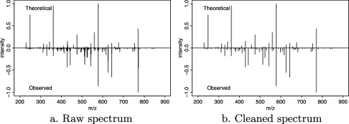
Figure 1: Observed and theoretical spectra of a charge 1$+$ peptide sequence LVTDLTK. In each plot, top panel is the theoretical spectrum predicted using our implementation based on Zhang (2004), and bottom panel is the observed spectrum. Each spectrum is rescaled by dividing by its highest peak for better visualization. (a) Raw spectrum. (b) Cleaned spectrum from our preprocessing procedure.

2.2 Preprocessing

Observed tandem mass spectra (specifically, those produced by LCQ or LTQ instruments) usually contain a large number of clustered peaks and low-intensity peaks, and have highly variable peak intensities [Figure 1(a)]. These factors pose challenges for developing statistical models. For example, clustered peaks often represent variants from the same fragmentation product (e.g., isotopic peaks) and so are not independent. Preprocessing has been reported to be important for the accuracy of peptide identification [Sun et al. (2007)].

Here we use a novel preprocessing procedure that attempts to distill the spectra down to the primary signals, normalizes the peak intensities on all theoretical and observed spectra to a comparable scale, and stabilizes peak intensities. In brief, the procedure distills the spectra down to the primary signals by clustering neighboring peaks and pooling near-by peaks into a single representative peak (Figure 1). Peak intensities in each cleaned spectrum are then normalized by dividing by the 90th percentile of the intensities of the peaks on the spectrum, to put the peaks from different spectra on a comparable scale. Finally, the normalized intensities are transformed by raising to 1$/$4 power to stabilize the highly variable intensities. We apply the same procedure to both theoretical and observed spectra before scoring. The preprocessing steps are described in detail in Table S1 in the supplementary materials [Li, Eng and Stephens (2012)].

2.3 A probabilistic model

We now outline the probabilistic model that is the central contribution of this paper. Let $\mathbf{T}=(T_{1},\ldots,T_{n})$ be a predicted theoretical spectrum with $n$ spectral peaks, where $T_{i}=(X_{i}^{t},Y_{i}^{t})$ denotes the location ($X^{t}_{i}$) and intensity ($Y^{t}_{i}$) for the $i$th peak, and $X^{t}_{i_{1}}\neq X^{t}_{i_{2}}$ if $i_{1}\neq i_{2}$. Similarly, let $\mathbf{O}=(O_{1},\ldots,O_{m})$ be an observed spectrum with $m$ spectral peaks, where $O_{j}=(X^{o}_{j},Y^{o}_{j})$ and $X^{o}_{j_{1}}\neq X^{o}_{j_{2}}$ if $j_{1}\neq j_{2}$. We find it convenient to assume that the peaks in $\mathbf{O}$ and $\mathbf{T}$ are arbitrarily ordered (i.e., they are randomly labeled $1,\ldots,n$ in $\mathbf{T}$ and $1,\ldots,m$ in $\mathbf{O}$), rather than being ordered by location, for example.

If $\mathbf{T}$ and $\mathbf{O}$ are generated from the same peptide sequence, then we view $\mathbf{O}$ as a distorted (i.e., noisy) realization of $\mathbf{T}$. Our aim here is to define a probability model $p_{\theta}(\mathbf{O}|\mathbf{T})$, depending on a set of parameters, $\theta$, described in detail below, that captures this distortion. [Actually, in specifying the probability model we condition on the number of peaks, $m$, in the observed spectrum, so $p_{\theta}(\mathbf{O}|\mathbf{T})$ should read $p_{\theta}(\mathbf{O}|\mathbf{T},m)$, but for notational simplicity we omit the explicit conditioning on $m$.]

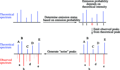
Figure 2: The probabilistic model for generating a random observed spectrum from a given theoretical spectrum, described in Section 2.3.

To specify this model, consider generating a random “observed” spectrum $\mathbf{O}$ from $p_{\theta}(\mathbf{O}|\mathbf{T})$ as follows (Figure 2): [(1)]

Each theoretical peak either does or does not “emit” an observed peak, independently for the $n$ theoretical peaks. We use $p_{i}$ to denote the probability that the $i$th theoretical peak, which with slight abuse of notation we abbreviate as $T_{i}$, emits a peak. We allow $p_{i}$ to depend on the intensity of $T_{i}$, so $p_{i}=g(Y^{t}_{i},\theta)$ for some function $g$, defined below. If $T_{i}$ emits a peak, then the location of the emitted peak is randomly sampled from a truncated normal distribution centered at $X_{i}^{t}$, and its intensity is randomly sampled from some distribution $f_{1}(\cdot;\theta)$.

Assume that the previous step produces $k$ emitted peaks, where $k\leq n\leq m$. (Typically, including every case we needed to consider in practical applications presented here, $n\leq m$.) Now generate $m-k$ additional “noise” peaks, so that the total number of peaks is $m$. These noise peaks have locations independently randomly sampled from a uniform distribution across the whole observable $m/z$ range, and intensities independently sampled from a distribution $f_{0}(\cdot;\theta)$. Note that, despite their name, these noise peaks may represent either measurement noise, or genuine peaks that were simply not included in $\mathbf{T}$ due to limitations of the theoretical prediction model.

Randomly label the observed peaks $1,\ldots,m$, uniformly on all possible labelings.

The above process is flexible enough to capture several important properties of real data. For example, by letting $p_{i}$ depend on the intensity of $T_{i}$, it captures the fact that high-intensity theoretical peaks are more likely to have matching observed peaks. And by allowing $f_{1}$ to be stochastically larger than $f_{0}$, it can take account of the fact that observed peaks that match a theoretical peak will tend to have higher intensities than other observed peaks (Figure 1). Here we assume that $g$ is a logistic function, and use histogram-like density estimates (i.e., piecewise constant densities) for $f_{0}$ and $f_{1}$, with parameters of these functions being estimated from data as described below.

The probability $p_{\theta}(\mathbf{O}|\mathbf{T})$ captures how probable it is that a peptide with theoretical spectrum $\mathbf{T}$ would have resulted in the observed spectrum $\mathbf{O}$, and is thus a suitable scoring function for comparing different candidate $\mathbf{T}$s to identify the peptide that created $\mathbf{O}$. However, although $p_{\theta}(\mathbf{O}|\mathbf{T})$, described above, is very easy to simulate from, it is tricky to compute for any given $\mathbf{T}$, because we do not observe which theoretical peak, if any, “emitted” each observed peak. So computing $p_{\theta}(\mathbf{O}|\mathbf{T})$ involves a computationally-intensive sum over all possibilities.

To formalize this model, let $\mathbf{e}$ denote the unobserved “emission configuration” which identifies which theoretical peaks emitted which observed peaks. Each emission configuration $\mathbf{e}$ determines an emission function $e^{t}$, with $e^{t}(i)=j$, ($j=1,\ldots,m$), if $T_{i}$ emits $O_{j}$, and $e^{t}(i)=0$ if $T_{i}$ does not emit any observed peak. Similarly, $\mathbf{e}$ also determines another emission function $e^{o}$, with $e^{o}(j)=i$, ($i=1,\ldots,n$), if $O_{j}$ is emitted from $T_{i}$, and $e^{o}(j)=0$ if $O_{j}$ is a noise peak. Note that $e^{t}(\cdot)$ and $e^{o}(\cdot)$ contain the same information.

Now, we can write $p_{\theta}(\mathbf{O}|\mathbf{T})$ as a sum over all possible values of $\mathbf{e}$:

$$p_{\theta}(\mathbf{O}|\mathbf{T})=\sum_{\mathbf{e}}\bigl{[}p_{\theta}(\mathbf{O}|\mathbf{T},\mathbf{e})p_{\theta}(\mathbf{e}|\mathbf{T})\bigr{]}.$$ (1)

Here

$$p_{\theta}(\mathbf{e}|\mathbf{T})=\frac{(m-k)!}{m!}\prod_{\{i:e^{t}(i)>0\}}g\bigl{(}Y^{t}_{i};\theta\bigr{)}\prod_{\{i:e^{t}(i)=0\}}\bigl{(}1-g\bigl{(}Y^{t}_{i};\theta\bigr{)}\bigr{)},$$ (2)

where $k\equiv|\{i\dvtx e^{t}(i)>0\}|=|\{j\dvtx e^{o}(j)>0\}|$ is the number of emission peaks; and

$$p_{\theta}(\mathbf{O}|\mathbf{T},\mathbf{e}) = \biggl{(}\frac{1}{r}\biggr{)}^{m-k}\prod_{\{j:e^{o}(j)=0\}}f_{0}\bigl{(}Y^{o}_{j}\bigr{)}$$

$${}\times\prod_{\{j:e^{o}(j)>0\}}\bigl{[}N_{T}\bigl{(}X^{o}_{j};X^{t}_{j},\sigma^{2},w\bigr{)}f_{1}\bigl{(}Y^{o}_{j}\bigr{)}\bigr{]},$$

where $r$ is the length of the $m/z$ range of the uniform distribution on noise peaks, and $N_{T}(x;\mu,\sigma^{2},w)$ denotes the truncated normal distribution, with mean $\mu$, variance $\sigma^{2}$, truncated at distance $w$ from the mean (here we assume that $w>0$ is a known constant reflecting the precision of the instrument).

Each term in the sum (1) is easy to compute. However, the number of terms is sufficiently large to create computational challenges (even when we take account of the fact that each emitted observed peak must be within $\pm w$ of the corresponding theoretical peak, which does substantially reduce the number of terms, and provides the primary motivation for using a truncated normal distribution rather than a nontruncated normal). To reduce the computation, we replace the likelihood (1) with the complete data likelihood under the most probable configuration, that is,

$$\hat{L}(\theta;\mathbf{O},\mathbf{T}):=\max_{\mathbf{e}}\bigl{[}p_{\theta}(\mathbf{O}|\mathbf{T},\mathbf{e})p_{\theta}(\mathbf{e}|\mathbf{T})\bigr{]}.$$ (4)

The procedure for searching the most probable configuration and estimating parameters is described in detail in Section 2.5. In general, the complete data likelihood (4) will be a good approximation to the likelihood (1) only if the sum in the latter is dominated by its single biggest term, which will not always be the case. Nonetheless, simulations (Section 3) and empirical evaluation presented below demonstrate that use of (4) produces good performance in practice.

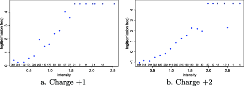
Figure 3: Exploratory data analysis shows an approximate linear trend between theoretical intensities and logit of empirical emission frequencies. The theoretical intensities are preprocessed as described in Section 2.2, and are binned (20 bins) with a fixed binwidth. The emission frequencies are estimated as the proportions of putative matches (i.e., the observed peaks and the theoretical peaks that locate less than 2 Daltons apart) in each bin from training data. To avoid overflow when all peaks in a bin form putative matches, $p$ is bounded at 0.99 at plotting (i.e., Y-axis is bounded at 4.69). The number of observations in each bin is marked at the bottom of the plot.

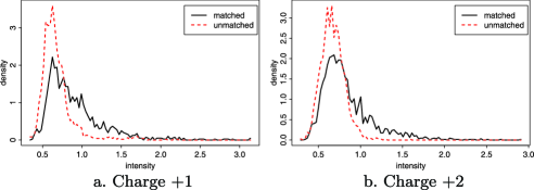
Figure 4: Empirical distributions of intensities for peaks on observed spectra. The emission status of each observed peak is approximated by whether there exists a theoretical peak that is less than 2 Da apart from the observed peak: Matched: observed peaks within 2 Da of a theoretical peak; Unmatched: other observed peaks. The observed intensities are normalized and transformed as described in Section 2.2 and are binned (100 bins) with even binwidth for plotting.

2.4 Choice of $g$, $f_{0}$ and $f_{1}$

As noted above, we assume that $g$ is a logistic function. That is, we allow $p_{i}$ to depend on $y^{t}_{i}$ using a logistic regression:

$$\log{\frac{p_{i}}{1-p_{i}}}=\mu+\beta y^{t}_{i}.$$ (5)

Here the intercept $\mu$ is assumed to be spectrum-specific to take account of the variation across spectra, and the slope $\beta$ is assumed to be common to all spectra. Exploratory data analysis (e.g., Figure 3) suggests that a logistic form for $g$ is reasonable for our data.

Empirical evaluations on the intensities of peaks on observed spectra show that both $f_{0}$ and $f_{1}$ are heavy-tailed distributions (Figure 4) where $f_{1}$ has a heavier right tail than $f_{0}$. Rather than make specific parametric assumptions regarding $f_{0}$ and $f_{1}$, we allow them to take flexible shapes by using piecewise-constant densities. For the data here, we made a specific choice of a piecewise-constant function of 10 bins, where the highest $1\%$ of the intensities of observed peaks in the training set is contained in the $10$th bin and the remaining $99\%$ are equally distributed in the remaining 9 bins. The same bin boundaries are used for $f_{0}$ and $f_{1}$. These parameters are assumed to be common to all spectra.

2.5 Parameter estimation, scoring and initialization

For the applications presented here we used a supervised approach to estimate the parameters of our probabilistic model, based on the availability of a training set of $N$ spectrum pairs $(\mathbf{O}_{s},\mathbf{T}_{s})\ (s=1,\ldots,N)$, where $\mathbf{O}_{s}$ and $\mathbf{T}_{s}$ are known to be generated from the same peptide. However, these parameters could also be estimated in other ways when training data are not available; see Discussion.

We write $\theta=(\theta_{0},\mu_{1},\ldots,\mu_{N})$ for the parameters to be estimated, where $\theta_{0}=(\sigma^{2},\beta,f_{0},f_{1})$ denotes parameters shared across all spectra pairs in (4), and $(\mu_{1},\ldots,\mu_{N})$ are spectrum-specific intercepts defined in (5). Using the training data, we estimate $\theta=(\theta_{0},\mu_{1},\ldots,\mu_{N})$ by

$$\hat{\theta}=\operatorname{argmax}\prod_{s}\hat{L}(\theta;\mathbf{O}_{s},\mathbf{T}_{s}).$$ (6)

When scoring a spectrum $\mathbf{T}$ for an observed spectrum $\mathbf{O}$, we then compute the score function

$$S(\mathbf{T};\mathbf{O}):=\max_{\mu}\hat{L}(\hat{\theta}_{0},\mu;\mathbf{O},\mathbf{T}),$$ (7)

using $\hat{\theta}_{0}$ estimated from the training stage. The spectra at different charge states are trained and scored separately.

Because the term $\hat{L}$ defined in (6) and (7) involves both $\mathbf{e}$ and $\theta$, the maximization involves simultaneously maximizing the configuration $\mathbf{e}$ and parameters. Detailed steps are described in Table 4 in the Appendix. As a configuration is updated only when the likelihood is increasing, this procedure guarantees the likelihood will be nondecreasing throughout the procedures. This procedure usually converged within 30 iterations for the data we tested.

2.6 Uncertainty of identifications

One advantage of our likelihood-based scoring approach is that it leads naturally to an assessment of the confidence that a given peptide generated a given spectrum. Specifically, if we assume that exactly one of the candidates generated the observed spectrum, and all are equally likely a priori, then by Bayes’ theorem the probability that $\mathbf{T}_{t}$ generated $\mathbf{O}$ is given by

$$P(\mathbf{T}_{t}|\mathbf{O})=\frac{p(\mathbf{O}|\mathbf{T}_{t})}{\sum_{i\in C_{o}}p(\mathbf{O}|\mathbf{T}_{i})},$$ (8)

where $C_{o}$ is the collection of candidate sequences for the observed spectrum $\mathbf{O}$. In practice, we use the scores $S(\mathbf{T};\mathbf{O})$ in place of $p(\mathbf{O}|\mathbf{T})$ to approximate this expression.

A nice feature of (8) is that it weighs the evidence for different candidates directly against each other, rather than against some null hypothesis, which often requires a large number of candidates to obtain reasonable estimates of uncertainty, as in, for example, Fenyo and Beavis (2003), Klammer, Park and Noble (2009). Thus, for example, if several good candidates provide similarly good matches to the observed spectrum $\mathbf{O}$, then we could not be confident which candidate generates $\mathbf{O}$ and this uncertainty is appropriately reflected in (8). [On the other hand, because equation (8) is based on an assumption that exactly one of the candidates produced the observed spectrum, it does not incorporate uncertainty due, for example, to the possibility that the database search entirely missed the correct spectrum. Empirically, however, we have found that the absence of the real sequence from the list of candidates tends not to cause a problem: in such cases confidence measures of all candidates tend to be low.]

3 Simulation

Here we use simulation studies to examine the performance of our approach, particularly to assess the accuracy of estimating parameters using the complete data likelihood (4) rather than the actual likelihood (1). To do so, we generate observed spectra from theoretical spectra using the probabilistic model described in Section 2.3, then estimate parameters and emission statuses by maximizing the complete data likelihood (4) using the estimation procedure in Section 2.5.

In an attempt to generate realistic simulations, we first estimate parameters from a training data of 50 charge $+$1 and 50 charge $+$2 spectra (described in Section 4) for each charge state, using the estimation procedure described in Section 2.5. We then simulate one observed spectrum from each theoretical spectrum in the training set using the estimated parameters, with $0.9n$ noise peaks on each observed spectrum, where $n$ is the number of theoretical peaks. We estimate the parameters and evaluate the accuracy of estimated emission status for each peak on the observed and theoretical spectra. The simulation is repeated 100 times.

The estimated parameters (Table 1) are close to the true values, which indicates the complete data likelihood at the most probable emission configuration provides adequate parameter estimates.

Table 1: Parameter estimation and accuracy of estimated emission status in simulated data. $\operatorname{CE}_{T}$ is the proportion of misclassified emission labels for peaks on the theoretical spectra after estimation, $\operatorname{CE}_{O}$ is the proportion of misclassified emission labels for peaks on the observed spectra after estimation. Each simulation consists of 50 theoretical spectra and their corresponding observed spectra simulated from the probabilistic model. Mean and standard deviation are computed based on 100 simulations

	Charge $\bolds{+1}$		Charge $\bolds{+2}$
	True	Estimated	True	Estimated
	parameter	from $\bolds{\hat{L}}$	parameter	from $\bolds{\hat{L}}$
$\mu$	$-1.240$	$-1.052$ (0.119)	$-5.060$	$-5.037$ (0.145)
$\beta$	$-$2.970	$-$2.929 (0.188)	$-$4.740	$-$4.785 (0.150)
$\sigma$	$-$0.390	$-$0.382 (0.008)	$-$0.160	$-$0.157 (0.003)
$\operatorname{CE}_{T}$	–	$-$0.046 (0.004)	–	$-$0.014 (0.002)
$\operatorname{CE}_{O}$	–	$-$0.049 (0.004)	–	$-$0.028 (0.003)

4 Applications

4.1 ISB data

To illustrate our approach, we applied it to a widely-used standard protein mixture, known as the ISB data, for assessing peptide identification [Keller et al. (2002a)]. This data set consists of the MS/MS spectra generated from a sample composed of trypsin digest of 18 purified proteins, including 504 charge $+$1 spectra, 18,496 charge $+$2 spectra and 18,044 charge $+$3 spectra. The spectra in the data set have been analyzed using SEQUEST [Eng, McCormack and Yates (1994)], a commonly-used software for peptide identification, and a list of 10–11 top-ranked candidates selected by SEQUEST was provided for each spectrum. For a subset of spectra, hand-curation (i.e., manual inspection) has confirmed that the top-ranked peptide assignment from SEQUEST is correct. This subset, which we refer to as the “hand-curated dataset” in what follows, consists of 125 $+$1 spectra, 1640 $+$2 spectra and 1010 $+$3 spectra. The experimental procedures are described in Keller et al. (2002a).

Because we implemented Zhang’s prediction model only for charge $+$1 and $+$2 peptides, here we consider only the observed spectra at these charge states, though our scoring method could also be applied to spectra at other charge states [Zhang (2005)]. As the resolution of the instrument to generate the spectra in this data set is about 2 Da [Wan, Yang and Chen (2006)], we set $w=2$ Da [e.g., in (2.3) and Table S1 in the supplementary materials [Li, Eng and Stephens (2012)].

Because of the computational cost involved in predicting theoretical spectra, the comparison is carried out on only the top 10 candidates selected by SEQUEST rather than all the candidates in the entire database. That is, we effectively assess the accuracy of a two-stage procedure that first selects candidates using SEQUEST, and then refines the ranking of the candidates shortlisted by SEQUEST using our likelihood-based score and the similarity index, respectively. Both theoretical spectra and observed spectra are preprocessed using the procedure described earlier (Table S1 in the supplementary materials [Li, Eng and Stephens (2012)]) prior to scoring with our method and the similarity index.

4.2 Other methods compared

We compare the results from our scoring method with the Xcorr score from SEQUEST and a similarity index (I) in Zhang (2004). SEQUEST is one of the most widely-used software for peptide identification. It scores candidate peptides using coarse theoretical spectra and reports multiple scores for each candidate peptide. XCorr score is the main filter score from SEQUEST, defined as $\operatorname{Xcorr}=R_{0}-\sum_{i=-75}^{i=75}R_{i}/151$, where $R_{i}$ is the cross-correlation between the theoretical spectrum and an observed spectrum with lag $i$ [Eng, McCormack and Yates (1994)]. The similarity index is defined as $I=\frac{\sum_{i}\sqrt{y^{o}_{i}y^{t}_{i}}}{\sqrt{\sum_{i}y_{i}^{o}}\sqrt{\sum_{i}y_{i}^{t}}}$, where $y^{o}_{i}$ and $y^{t}_{i}$ are the peak intensities at (discretized) $m/z$ location $i$ on observed and theoretical spectra, respectively. It was originally proposed in Zhang (2004) for assessing the similarity between a refined theoretical spectrum generated from the kinetic model in Zhang (2004) and its corresponding observed spectrum, and recently was used, in conjunction with other heuristic rules, to validate top-ranked identifications made by common database search algorithms using refined theoretical predictions [Sun et al. (2007), Yu et al. (2010)].

4.3 Evaluation on the curated data set

We first evaluate the performance of our method and the similarity index on the hand-curated data set. Because, by construction, this data set includes only spectra that were correctly identified by SEQUEST, we cannot make meaningful comparisons with SEQUEST on these data. For our method, for each charge state, 50 observed spectra are randomly selected as training data, and the remaining spectra are used for testing (resulting in test sets of size 75 for charge $+$1 and 1590 for charge $+$2). No training is needed for computing the similarity index. It is known that mass spectrometry has difficulty distinguishing several sets of amino acids due to their close or identical mass. Specifically, Ile and Leu have identical mass, and Lys is difficult to distinguish from Gln. To allow for these undistinguishable variants, in assessing each method’s performance on this subset, we call an identification correct if the peptide candidate receiving the highest score agrees either with the hand-curated choice or with an undistinguishable variant (i.e., a variant that swaps Ile with Leu and/or Lys with Gln).

Table 2: Correct identification rate on the curated ISB data set. The confident subset consists of testing spectra whose top candidates are highly confident, that is, $P(\mathbf{T}_{\mathrm{top}}|\mathbf{O})\geq 99\%$

		Charge $\bolds{+1}$	Charge $\bolds{+2}$	All
Likelihood score $(S)$	train	94.0% ($n=50$)	100.0% ($n=50$)000	97.0% ($n=100$)0
	test	93.3% ($n=75$)	96.8% ($n=1590$)	96.6% ($n=1665$)
	confident subset	98.3% ($n=58$)	98.7% ($n=1492$)	98.7% ($n=1550$)
Similarity index $(I)$	test	78.7% ($n=75$)	88.0% ($n=1590$)	87.6% ($n=1665$)

Average identification accuracy. Table 2 summarizes identification accuracy for these data. Our model correctly identifies most spectra (96.6% of the spectra in the test set) and performs markedly better than the similarity index (87.6% correct on test set).

High-confidence subsets and calibration of posterior probabilities. Besides providing accurate average performance, two other features of a method are desirable. First, it should provide a meaningful ranking of confidence in different identifications. In particular, it would be helpful if the method were able to identify a subset of high confidence identifications that are highly likely to be correct. Second, it should provide a calibrated assessment of confidence in each individual identification: in our case, one would like the probabilities assigned to individual identifications to be calibrated, so that, for example, of identifications assigned 50% probability of being correct, around half are actually correct.

Figure 5: False discovery rate versus undetermined rate for the test data in ISB curated data set. Shown is the comparison between posterior probability from our method (solid line) and the difference in the similarity index between the best and second-best identifications (dashed line).

For these data, our method exhibits both of these desirable properties. First, among identifications scored with the highest confidence by our method ($P(\mathbf{T}|\mathbf{O})\geq 0.99$), 98.7% of spectra are correctly identified (Table 2). Of course, restricting attention to this class of high-confidence calls reduces the overall number of spectra identified: in this case, 93.1% of spectra fall into our high-confidence category, so when we use a calling threshold of $0.99$, $6.9\%$ of spectra are “undetermined.” Figure 5 shows the general trade-off between identification accuracy (actually, False Discovery Rate) and undetermined rate, as the calling threshold changes. For comparison, Figure 5 also shows the same trade-off for the similarity index, with confidence in each call measured by the difference in the similarity index between the best and second-best identifications. Although the similarity index is able to provide some meaningful ranking of confidence in each call—as indicated by the lower FDR at more stringent thresholds—the FDR at any given undetermined rate is consistently higher than for our method.

Turning to calibration, Figure 6 shows the calibration of posterior probabilities from our model. To produce this plot, we took all candidate sequences in this data set (not just the top-ranked sequences) and grouped them into bins by their posterior probabilities. Within each bin we compared the posterior probabilities with the empirical correct identification rate. The approximate linear trend in Figure 6 shows that, for these data, our method provides reasonably well calibrated probability assessments in both charge states. The ability to produce well-calibrated probabilities of correct identifications is a potential advantage of using likelihood-based scoring rules such as the one we present here, compared with similiarity-based scoring rules that do not naturally lead to probabilistic assessments of correctness.

Figure 6: Calibration of posterior probabilities in ISB curated data set. The observations are binned by the assigned probabilities. For each bin, the assigned probabilities (X-axis) are compared with the proportion of identifications that are actually correct (Y-axis). The dashed line marks perfect calibration. The number of observations at each point is marked at the bottom of the plot.

4.4 Comparisons with SEQUEST: The benefit of refining identifications

In this section we evaluate the benefit of using our likelihood-based score to refine identifications made by SEQUEST, by comparing the results of our method with (unrefined) SEQUEST results, and with the similarity index. Again, because the hand-curated data consists only of identifications that are correctly identified by SEQUEST, it cannot be used to make meaningful comparisons with SEQUEST. Instead, we form a different subset of the ISB data for comparison, based on the fact that these spectra were generated from a known mixture of proteins. Specifically, we take the subset of the (test-set) spectra whose top 10 candidates selected by SEQUEST include at least one subsequence of a constituent protein in the known protein mixture. The resulting subset contains 504 charge $+$1 spectra and 3669 charge $+$2 spectra. When assessing a peptide identification for each spectrum, the assumption we make, standard in this context, is that the identified peptide is correct if and only if its amino acid sequence is a subsequence of a constituent protein in the known mixture.

Table 3: Correct identification rate for the spectra whose top 10 candidate sequencesselected by SEQUEST include subsequence(s) of the constituent proteinsin the ISB data. The confident subset consists of testing spectra whose top candidates are highly confident, that is, $P(\mathbf{T}_{\mathrm{top}}|\mathbf{O})\geq 99\%$

		Charge $\bolds{+1}$	Charge $\bolds{+2}$	All
Likelihood score $(S)$	test	86.9% ($n=504$)	87.7% ($n=3669$)	87.6% ($n=4173$)
	confident subset	99.1% ($n=346$)	98.0% ($n=3008$)	98.1% ($n=3354$)
SEQUEST	test	68.1% ($n=504$)	82.0% ($n=3669$)	80.2% ($n=4173$)
Similarity index $(I)$	test	60.7% ($n=504$)	76.3% ($n=366$9)	74.4% ($n=4173$)

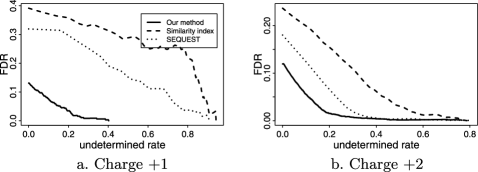
Figure 7: False discovery rate versus undetermined rate for the spectra whose top 10 candidates selected by SEQUEST include subsequence(s) of the constituent proteins in the ISB data. Shown is the comparison between posterior probability computed using our method (solid line), the difference in the similarity index between the best and second-best identifications (dashed line) and Delta Cn of SEQUEST (dotted line), which is the normalized difference between the top two Xcorr values. Xcorr performs worse than Delta Cn in this data set, thus it is not shown.

In this data set, our method correctly identifies substantially more real peptides than SEQUEST and the similarity index (I) for both charge $+$1 and charge $+$2 spectra (Table 3). Among them, our method not only correctly identifies most spectra that SEQUEST correctly identifies, but also identifies many of the spectra that are misidentified by SEQUEST. Similar to the hand-curated data set, here our method is also able to identify a subset of high-confidence high-accuracy identifications (e.g., 98.1% of spectra are correctly identified on this subset, see Table 3) and provides a substantially lower false discovery rate than both SEQUEST and the similarity index at any given undetermined rate (Figure 7).

The gain of using our method to refine SEQUEST results is noticeably higher for charge $+$1 spectra than for charge $+$2 spectra. Sun et al. (2007) also observed a higher gain in charge $+$1 spectra when using the more refined theoretical spectra for peptide identification using similarity index in conjunction with a series of heuristic rules. They interpreted this as being due to the fact that charge $+$1 spectra tend to follow minor fragmentation pathways, which are excluded in the coarse theoretical spectra but included in the refined theoretical spectra, more frequently than charge $+$2 spectra [Wysocki et al. (2000)], so refined theoretical spectra tend to fill in more information that coarse theoretical spectra miss on charge $+$1 spectra.

We also note that the similarity index identifies fewer real peptides than SEQUEST in our study. This is different from the results in Sun et al. (2007), who showed more favorable performance for the similarity score compared with SEQUEST, when refining the top-ranked peptides identified by SEQUEST, and MASCOT, another widely-used peptide identification algorithm, using the similarity scores, in conjunction with other heuristic rules. This disparity could be attributed to a number of differences between their study and ours, such as selection criteria for test spectra (their selection criteria for test spectra enrich for spectra that are easy to discriminate and also involve filtering using the similarity index itself), choice of test data sets, preprocessing procedures (including data transformation) and their use of additional heuristic rules.

5 Discussion

We have developed a likelihood-based scoring approach to peptide identification using a database search. This method is based on a rigorous statistical model, which provides a flexible framework to model the fine details and noise structure in the spectra. By taking account of multiple sources of noise in the spectra using a model-based approach, the method makes use of the information of peak intensities on both observed spectra and theoretical spectra predicted by sophisticated chemical principles, in addition to peak locations, in scoring peptide-spectrum matches. Moreover, the use of a likelihood-based score leads naturally to an assessment of the probability that each individual identification is correct. In the ISB data we examined here, the probabilities produced by our method were well-calibrated and produced better identification accuracy than SEQUEST or the similarity index.

Our results confirm that finer-scale spectra predicted from comprehensive fragmentation pathways can provide valuable information for peptide identification [Sun et al. (2007)] and demonstrate the potential to improve the accuracy of spectra matching by modeling these structures. Similar improvement in peptide identification was also observed in Klammer et al. (2008), who developed a probabilistic model of peptide fragmentation chemistry using the dynamic Bayesian network (DBN) and identified peptides using the features learned from DBN using the support vector machine (SVM). Similar to Zhang (2004), Klammer et al. (2008) incorporated peptide fragmentation chemistry using the widely accepted mobile proton model [Dongre et al. (1996), Wysocki et al. (2000)]. It then trained DBNs using positive and negative spectra and generated a set of DBNs to capture the probabilistic relationships governing fragment intensities. Unlike Zhang (2004), it does not produce a theoretical spectrum for each peptide candidate; instead, it yields for each peptide-spectrum match a vector of features from each DBN to be discriminated by the SVM. One advantage of the likelihood-based scoring method over the SVM approach is that it can assess the uncertainty of identification for each identified peptide relative to other candidate peptides for the same observed spectra.

Although we have focussed here on using the likelihood-based score for improving accuracy of peptide identification by peptide database search, it could also be usefully integrated into many other proteomics analyses that exploit such scores. For example, our score could be easily applied to a spectral library search [Lam et al. (2007)], where query spectra are identified by matching to a library of previously annotated observed spectra. Here the fact that our score models the fine structure on both query and library spectra should be expected to improve accuracy compared with simpler scoring algorithms. Similarly, peptide-spectrum match scores from our method could be used as input to software that use such scores in downstream analyses, such as identifying the proteins that are likely present in a mixture [Gerster et al. (2010), Keller et al. (2002b), Li, MacCoss and Stephens (2010), Nesvizhskii and Aebersold (2004), Shen et al. (2008)]. The improved performance we observed for the likelihood-based score in the peptide identification problem, compared with other scoring rules, should be expected to translate to improved accuracy of downstream protein identification.

Table 4: Procedure for estimating parameters and scoring

Let $(T,O)$ denote a pair of theoretical and observed spectra in the training set. For each such pair, do 1(a) and 1(b). [(1)] (1) Initialization: [(a)] (a) Recall, from the main paper, that $e$ denotes the unobserved “emission configuration” that maps each peak in $T$ to the peak it gave rise to in $O$ (or to no peak if it gave rise to no observed peak). Here we generate a set $E$ containing all possible values for $e$. [(iii)] (i) For each $T_{i}$, $i=1,\ldots,n$, find $\hat{e}^{o}(\{i\})$. (ii) If $\hat{e}^{o}(\{i_{1}\})\cap\hat{e}^{o}(\{i_{2}\})\neq\varnothing$ for some $i_{1}$ and $i_{2}\in\{1,\ldots,n\}$, merge both the index sets and the mapped sets, and obtain $\hat{e}^{o}(\{i_{1},i_{2}\})=\hat{e}^{o}(\{i_{1}\})\cup\hat{e}^{o}(\{i_{2}\})$. (iii) Repeat merging, until all mapped sets are mutually exclusive. Suppose $G$ mutually exclusive sets are obtained with corresponding sets of theoretical peaks indexed by $I_{1},\ldots,I_{G}$. The emission configurations of peaks within each putative emission set $(I_{g},\hat{e}^{o}(I_{g}))$, $g=1,\ldots,G$, are determined only by peaks within the set and are independent of peaks in other sets. (iv) Let $e_{g}$ denote the emission configuration $e$ restricted to the set of theoretical peaks in $I_{g}$. Thus, $e_{g}$ maps each theoretical peak in $I_{g}$ to $\hat{e}^{o}(I_{g})$. Enumerate all possible values for $e_{g}$, and call this set $E_{g}$. (b) Generate an initial configuration to start Step 2: [(i)] (i) For each putative emission set $g$, assign $e_{g}^{0}=\operatorname{argmin}_{i\in I_{g},j\in\hat{e}^{o}(I_{g})}|T_{i}-O_{j}|$. Denote the initial configuration as $\mathbf{e}^{0}=(e^{0}_{1},\ldots,e^{0}_{G})$. (2) Maximization: In this section we use the subscript $s$ to label the different spectra in the training set. So the training set consists of pairs $\{(T_{s},O_{s})\dvtx s=1,\ldots,S\}$ and $e_{s}$ denotes an emission configuration mapping peaks in $T_{s}$ to peaks in $O_{s}$. Alternate 2(a) and 2(b) until the log-likelihood $\sum_{s=1}^{N}\log L(\theta_{0},\mu_{1},\ldots,\mu_{N})$ converges: [(a)] (a) Estimate spectrum-nonspecific parameters $\theta_{0}$: [(i)] (i) $\hat{\theta}_{0}^{(t)}=\operatorname{argmax}_{\theta_{0}}\sum_{s}\log L((\theta_{0},\mu_{1},\ldots,\mu_{N})|\mathbf{O}_{s},\mathbf{T}_{s},\mathbf{e}_{s}^{(t)})$) for current $\mathbf{e}^{(t)}_{s}=(e^{(t)}_{s,1},\ldots,e^{(t)}_{s,G})$. (b) Update configuration and estimate $\mu_{s}$: For each pair of spectra $\mathbf{T}_{s}$ and $\mathbf{O}_{s}$, repeat 2b(i-ii) until $\log L((\hat{\theta}_{0},\mu_{s})|\mathbf{O}_{s},\mathbf{T}_{s},\mathbf{e}^{(t)}_{s})$ converges. [(ii)] (i) Generate a random permutation $\phi=(\phi_{1},\ldots,\phi_{G})$ of $(1,\ldots,G)$. (ii) Repeat for $g=1$ to $G$: [(A)] (A) Fix current configurations $e^{(t)}_{s,\phi_{1}},\ldots,e^{(t)}_{s,\phi_{g-1}},e^{(t)}_{s,\phi_{g+1}},\ldots,e^{(t)}_{s,\phi_{G}}$. For each $e_{s,\phi_{g}}\in E_{\phi_{g}}$, define $\mathbf{e}_{s,\phi_{g}}^{(t)}=e^{(t)}_{s,\phi_{1}},\ldots,e^{(t)}_{s,\phi_{g-1}},e_{s,\phi_{g}},e^{(t)}_{s,\phi_{g+1}},\ldots,e^{(t)}_{s,\phi_{G}}$, compute $\hat{\mu}_{s}$= $\operatorname{argmax}_{\mu_{s}}L((\theta_{0},\mu_{s})|\mathbf{O}_{s},\mathbf{T}_{s},\mathbf{e}_{s,g}^{(t)})$. (B) Update $e^{(t+1)}_{s,\phi_{g}}=\operatorname{argmax}_{e_{s,\phi_{g}}\in E_{g}}L((\theta_{0},\hat{\mu}_{s})|\mathbf{O}_{s},\mathbf{T}_{s},\mathbf{e}_{s,\phi_{g}}^{(t)})$

While the work described here provides a solid foundation for a rigorous statistical approach to the problem of matching spectra to their generating peptides, there remain many opportunities for further development and refinement. For example, one issue that would need to be tackled in practical applications is how to estimate parameters of the model in the absence of a training set. While simply using parameters estimated from the ISB data used here might perform adequately in some cases, one could almost certainly do better using data generated in the specific context of the experiment to be analyzed. One simple possibility worth investigating would be to use the most confident matches identified by a simpler approach, such as SEQUEST, as a training set; more statistically rigorous approaches, based, for example, on using an EM algorithm [Dempster, Laird and Rubin (1977)] to learn from unlabeled data, could also be developed. While the need to estimate parameters may initially seem like a drawback, it is also responsible for an important advantage of likelihood-based scores: specifically, it makes the likelihood-based score easily adaptable to the varying characteristics of spectra under, for example, different charge states and different machine instrumentation and settings.

Our method requires more computing than some other methods, such as the similarity score and Xcorr, because it involves optimizing the likelihood. The computational cost for identifying each peptide spectrum match is linear in the number of peaks on a cleaned spectrum. With our prototyping implementation in R, it takes on average 0.6 s and 1.4 s to evaluate each peptide spectrum match for charge 1$+$ and charge 2$+$ spectra, respectively. An implementation in C is expected to significantly improve the speed and makes it more suitable for practical use. A software implementation of the scoring algorithm described here is available from the first author on request.

Appendix: Estimation and scoring procedure

For any subset $I$ of theoretical peaks, let $\hat{e}^{o}(I)$ denote the set of observed peaks that could have been generated by the theoretical peaks in $I$. That is,

$$\hat{e}^{o}(I)=\bigcup_{i\in I}\bigl{\{}j\in\{1,\ldots,m\}\dvtx|T_{i}-O_{j}|\leq w\bigr{\}},$$ (9)

where $I$ is an index set for theoretical peaks. Also, define

$$L\bigl{(}(\theta_{0},\mu_{1},\ldots,\mu_{N})|\mathbf{O},\mathbf{T},\mathbf{e}\bigr{)}=p_{\theta}(\mathbf{O}|\mathbf{T},\mathbf{e})p_{\theta}(\mathbf{e}|\mathbf{T}).$$ (10)

Table 4 describes the procedure for estimating parameters and scoring. In the training stage, the entire procedure is carried out. When scoring spectra in the test set, step 2(a) is omitted and $\hat{\theta}_{0}$ estimated from the training stage is used.

References

- Coon et al. (2005) {barticle}[auto:STB—2012/06/08—12:49:54] \bauthor\bsnmCoon, \bfnmJ. J.\binitsJ. J., \bauthor\bsnmSyka, \bfnmJ. E.\binitsJ. E., \bauthor\bsnmShabanowitz, \bfnmJ.\binitsJ. and \bauthor\bsnmHunt, \bfnmD.\binitsD. (\byear2005). \btitleTandem mass spectrometry for peptide and proteins sequence analysis. \bjournalBioTechniques \bvolume38 \bpages519–521. \bptokimsref \endbibitem
- Dempster, Laird and Rubin (1977) {barticle}[mr] \bauthor\bsnmDempster, \bfnmA. P.\binitsA. P., \bauthor\bsnmLaird, \bfnmN. M.\binitsN. M. and \bauthor\bsnmRubin, \bfnmD. B.\binitsD. B. (\byear1977). \btitleMaximum likelihood from incomplete data via the EM algorithm. \bjournalJ. Roy. Statist. Soc. Ser. B \bvolume39 \bpages1–38. \bidissn=0035-9246, mr=0501537 \bptnotecheck related\bptokimsref \endbibitem
- Dongre et al. (1996) {barticle}[auto:STB—2012/06/08—12:49:54] \bauthor\bsnmDongre, \bfnmA. R.\binitsA. R., \bauthor\bsnmJohns, \bfnmJ. L.\binitsJ. L., \bauthor\bsnmSomogyi, \bfnmA.\binitsA. and \bauthor\bsnmWysocki, \bfnmV.\binitsV. (\byear1996). \btitleInfluence of peptide composition, gass-phase basicity, and chemical modification on fragmentation efficiency: Evidence for the mobile proton model. \bjournalJ. Am. Chem. Soc. \bvolume118 \bpages8365–8374. \bptokimsref \endbibitem
- Elias and Gygi (2007) {barticle}[auto:STB—2012/06/08—12:49:54] \bauthor\bsnmElias, \bfnmJ.\binitsJ. and \bauthor\bsnmGygi, \bfnmS.\binitsS. (\byear2007). \btitleTarget-decoy search strategy for increased confidence in large-scale protein identifications by mass spectrometry. \bjournalNature Methods \bvolume4 \bpages207–214. \bptokimsref \endbibitem
- Eng, McCormack and Yates (1994) {barticle}[auto:STB—2012/06/08—12:49:54] \bauthor\bsnmEng, \bfnmJ.\binitsJ., \bauthor\bsnmMcCormack, \bfnmA.\binitsA. and \bauthor\bsnmYates, \bfnmJ. I.\binitsJ. I. (\byear1994). \btitleAn approach to correlate tandem mass spectral data of peptides with amino acid sequences in a protein database. \bjournalJ. Am. Soc. Mass Spectrom \bvolume5 \bpages976–989. \bptokimsref \endbibitem
- Fenyo and Beavis (2003) {barticle}[auto:STB—2012/06/08—12:49:54] \bauthor\bsnmFenyo, \bfnmD.\binitsD. and \bauthor\bsnmBeavis, \bfnmR.\binitsR. (\byear2003). \btitleA method for assessing the statistical significance of mass spectrometry-based protein identifications using general scoring schemes. \bjournalAnal. Chem. \bvolume75 \bpages768–774. \bptokimsref \endbibitem
- Gerster et al. (2010) {barticle}[auto:STB—2012/06/08—12:49:54] \bauthor\bsnmGerster, \bfnmS.\binitsS., \bauthor\bsnmQeli, \bfnmE.\binitsE., \bauthor\bsnmAhrens, \bfnmC. H.\binitsC. H. and \bauthor\bsnmBuehlmann, \bfnmP.\binitsP. (\byear2010). \btitleProtein and gene model inference based on statistical modeling in k-partite graphs. \bjournalProc. Natl. Acad. Sci. USA \bvolume107 \bpages12101–12106. \bptokimsref \endbibitem
- Hernandez, Muller and Appel (2006) {barticle}[auto:STB—2012/06/08—12:49:54] \bauthor\bsnmHernandez, \bfnmP.\binitsP., \bauthor\bsnmMuller, \bfnmM.\binitsM. and \bauthor\bsnmAppel, \bfnmR. D.\binitsR. D. (\byear2006). \btitleAutomated protein identification by tandem mass spectrometry: Issues and strategies. \bjournalMass Spectrometry Reviews \bvolume25 \bpages235–254. \bptokimsref \endbibitem
- Keller et al. (2002a) {barticle}[pbm] \bauthor\bsnmKeller, \bfnmAndrew\binitsA., \bauthor\bsnmPurvine, \bfnmSamuel\binitsS., \bauthor\bsnmNesvizhskii, \bfnmAlexey I.\binitsA. I., \bauthor\bsnmStolyar, \bfnmSergey\binitsS., \bauthor\bsnmGoodlett, \bfnmDavid R.\binitsD. R. and \bauthor\bsnmKolker, \bfnmEugene\binitsE. (\byear2002a). \btitleExperimental protein mixture for validating tandem mass spectral analysis. \bjournalOMICS \bvolume6 \bpages207–212. \biddoi=10.1089/153623102760092805, issn=1536-2310, pmid=12143966 \bptokimsref \endbibitem
- Keller et al. (2002b) {barticle}[auto:STB—2012/06/08—12:49:54] \bauthor\bsnmKeller, \bfnmA.\binitsA., \bauthor\bsnmNesvizhskii, \bfnmA.\binitsA., \bauthor\bsnmKolker, \bfnmE.\binitsE. and \bauthor\bsnmAebersold, \bfnmR.\binitsR. (\byear2002b). \btitleEmpirical statistical model to estimate the accuracy of peptide identifications made by ms/ms and database search. \bjournalAnal. Chem. \bvolume74 \bpages5383–5392. \bptokimsref \endbibitem
- Kinter and Sherman (2000) {bbook}[auto:STB—2012/06/08—12:49:54] \bauthor\bsnmKinter, \bfnmM.\binitsM. and \bauthor\bsnmSherman, \bfnmN. E.\binitsN. E. (\byear2000). \btitleProtein Sequencing and Identification Using Tandem Mass Spectrometry. \bpublisherWiley, \baddressNew York. \bptokimsref \endbibitem
- Klammer, Park and Noble (2009) {barticle}[auto:STB—2012/06/08—12:49:54] \bauthor\bsnmKlammer, \bfnmA. A.\binitsA. A., \bauthor\bsnmPark, \bfnmC. Y.\binitsC. Y. and \bauthor\bsnmNoble, \bfnmW. S.\binitsW. S. (\byear2009). \btitleStatistical calibration of the SEQUEST XCorr function. \bjournalJournal of Proteome Research \bvolume8 \bpages2106–2113. \bptokimsref \endbibitem
- Klammer et al. (2008) {barticle}[auto:STB—2012/06/08—12:49:54] \bauthor\bsnmKlammer, \bfnmA. A.\binitsA. A., \bauthor\bsnmReynolds, \bfnmS.\binitsS., \bauthor\bsnmMacCoss, \bfnmM. J.\binitsM. J., \bauthor\bsnmBilmes, \bfnmJ.\binitsJ. and \bauthor\bsnmNoble, \bfnmW.\binitsW. (\byear2008). \btitleModelling peptide fragmentation with dynamic Bayesian networks for peptide identification. \bjournalBioinformatics \bvolume24 \bpagesi348–i356. \bptokimsref \endbibitem
- Lam et al. (2007) {barticle}[auto:STB—2012/06/08—12:49:54] \bauthor\bsnmLam, \bfnmH.\binitsH., \bauthor\bsnmDeutsch, \bfnmE. W.\binitsE. W., \bauthor\bsnmEddes, \bfnmJ. S.\binitsJ. S., \bauthor\bsnmEng, \bfnmJ. K.\binitsJ. K., \bauthor\bsnmKing, \bfnmN.\binitsN., \bauthor\bsnmStein, \bfnmS. E.\binitsS. E. and \bauthor\bsnmAebersold, \bfnmR.\binitsR. (\byear2007). \btitleDevelopment and validation of a spectral library searching method for peptide identification from MS/MS. \bjournalProteomics \bvolume7 \bpages655–667. \bptokimsref \endbibitem
- Li, Eng and Stephens (2012) {bmisc}[auto:STB—2012/06/08—12:49:54] \bauthor\bsnmLi, \bfnmQ.\binitsQ., \bauthor\bsnmEng, \bfnmJ. K.\binitsJ. K. and \bauthor\bsnmStephens, \bfnmM.\binitsM. (\byear2012). \bhowpublishedSupplement to “A likelihood-based scoring method for peptide identification using mass spectrometry.” DOI:\doiurl10.1214/12-AOAS568SUPP. \bptokimsref \endbibitem
- Li, MacCoss and Stephens (2010) {barticle}[mr] \bauthor\bsnmLi, \bfnmQunhua\binitsQ., \bauthor\bsnmMacCoss, \bfnmMichael J.\binitsM. J. and \bauthor\bsnmStephens, \bfnmMatthew\binitsM. (\byear2010). \btitleA nested mixture model for protein identification using mass spectrometry. \bjournalAnn. Appl. Stat. \bvolume4 \bpages962–987. \biddoi=10.1214/09-AOAS316, issn=1932-6157, mr=2758429 \bptokimsref \endbibitem
- Nesvizhskii and Aebersold (2004) {barticle}[auto:STB—2012/06/08—12:49:54] \bauthor\bsnmNesvizhskii, \bfnmA. I.\binitsA. I. and \bauthor\bsnmAebersold, \bfnmR.\binitsR. (\byear2004). \btitleAnalysis, statistical validation and dissermination of large-scale proteomics datasets generated by tandem ms. \bjournalDrug Discovery Today \bvolume9 \bpages173–181. \bptokimsref \endbibitem
- Nesvizhskii et al. (2003) {barticle}[auto:STB—2012/06/08—12:49:54] \bauthor\bsnmNesvizhskii, \bfnmA.\binitsA., \bauthor\bsnmKeller, \bfnmA.\binitsA., \bauthor\bsnmKolker, \bfnmE.\binitsE. and \bauthor\bsnmAebersold, \bfnmR.\binitsR. (\byear2003). \btitleA statistical model for identifying proteins by tandem mass spectrometry. \bjournalAnal. Chem. \bvolume75 \bpages4646–4653. \bptokimsref \endbibitem
- Sadygov, Liu and Yates (2004) {barticle}[auto:STB—2012/06/08—12:49:54] \bauthor\bsnmSadygov, \bfnmR.\binitsR., \bauthor\bsnmLiu, \bfnmH.\binitsH. and \bauthor\bsnmYates, \bfnmJ.\binitsJ. (\byear2004). \btitleStatistical models for protein validation using tandem mass spectral data and protein amino acid sequence databases. \bjournalAnal. Chem. \bvolume76 \bpages1664–1671. \bptokimsref \endbibitem
- Shen et al. (2008) {barticle}[auto:STB—2012/06/08—12:49:54] \bauthor\bsnmShen, \bfnmC.\binitsC., \bauthor\bsnmWang, \bfnmZ.\binitsZ., \bauthor\bsnmShankar, \bfnmG.\binitsG., \bauthor\bsnmZhang, \bfnmX.\binitsX. and \bauthor\bsnmLi, \bfnmL.\binitsL. (\byear2008). \btitleA hierarchical statistical model to assess the confidence of peptides and proteins inferred from tandem mass spectrometry. \bjournalBioinformatics \bvolume24 \bpages202–208. \bptokimsref \endbibitem
- Sun et al. (2007) {barticle}[auto:STB—2012/06/08—12:49:54] \bauthor\bsnmSun, \bfnmS.\binitsS., \bauthor\bsnmMeyer-Arendt, \bfnmK.\binitsK., \bauthor\bsnmEichelberger, \bfnmB.\binitsB., \bauthor\bsnmBrown, \bfnmR.\binitsR., \bauthor\bsnmYen, \bfnmC.\binitsC., \bauthor\bsnmOld, \bfnmW.\binitsW., \bauthor\bsnmPierce, \bfnmK.\binitsK., \bauthor\bsnmCios, \bfnmK.\binitsK., \bauthor\bsnmAhn, \bfnmN. G.\binitsN. G. and \bauthor\bsnmResing, \bfnmK. A.\binitsK. A. (\byear2007). \btitleImproved validation of peptide ms/ms assignments using spectral intensity prediction. \bjournalMolecular and Cellular Proteomics \bvolume6 \bpages1–17. \bptokimsref \endbibitem
- Wan, Yang and Chen (2006) {barticle}[auto:STB—2012/06/08—12:49:54] \bauthor\bsnmWan, \bfnmY.\binitsY., \bauthor\bsnmYang, \bfnmA.\binitsA. and \bauthor\bsnmChen, \bfnmT.\binitsT. (\byear2006). \btitlePepHMM: A hidden Markov model based scoring function for mass spectrometry database search. \bjournalAnal. Chem. \bvolume78 \bpages432–437. \bptokimsref \endbibitem
- Wysocki et al. (2000) {barticle}[auto:STB—2012/06/08—12:49:54] \bauthor\bsnmWysocki, \bfnmV. H.\binitsV. H., \bauthor\bsnmTsaprsilis, \bfnmG.\binitsG., \bauthor\bsnmSmith, \bfnmL.\binitsL. and \bauthor\bsnmBreci, \bfnmL. A.\binitsL. A. (\byear2000). \btitleMobile and localized protons: A framework for understanding peptide dissociation. \bjournalJ. Mass Spectrom. \bvolume35 \bpages1399–1406. \bptokimsref \endbibitem
- Yen et al. (2011) {barticle}[auto:STB—2012/06/08—12:49:54] \bauthor\bsnmYen, \bfnmC.\binitsC., \bauthor\bsnmHouel, \bfnmS.\binitsS., \bauthor\bsnmAhn, \bfnmN. G.\binitsN. G. and \bauthor\bsnmOld, \bfnmW.\binitsW. (\byear2011). \btitleSpectrum-to-spectrum searching using a proteome-wide spectral library. \bjournalMol. Cell. Proteomics \bvolume10 \bpagesM111.007666. \bptokimsref \endbibitem
- Yu et al. (2010) {barticle}[auto:STB—2012/06/08—12:49:54] \bauthor\bsnmYu, \bfnmW.\binitsW., \bauthor\bsnmTaylor, \bfnmJ. A.\binitsJ. A., \bauthor\bsnmDavis, \bfnmM. T.\binitsM. T., \bauthor\bsnmBonilla, \bfnmL. E.\binitsL. E., \bauthor\bsnmLee, \bfnmK. A.\binitsK. A., \bauthor\bsnmAuger, \bfnmP. L.\binitsP. L., \bauthor\bsnmFarnsworth, \bfnmC. C.\binitsC. C., \bauthor\bsnmWelcher, \bfnmA. A.\binitsA. A. and \bauthor\bsnmPatterson, \bfnmS. D.\binitsS. D. (\byear2010). \btitleMaximizing the sensitivity and reliability of peptide identification in large-scale proteomic experiments by harnessing multiple search engines. \bjournalProteomics \bvolume10 \bpages1172–1189. \bptokimsref \endbibitem
- Zhang (2004) {barticle}[pbm] \bauthor\bsnmZhang, \bfnmZhongqi\binitsZ. (\byear2004). \btitlePrediction of low-energy collision-induced dissociation spectra of peptides. \bjournalAnal. Chem. \bvolume76 \bpages3908–3922. \biddoi=10.1021/ac049951b, issn=0003-2700, pmid=15253624 \bptokimsref \endbibitem
- Zhang (2005) {barticle}[pbm] \bauthor\bsnmZhang, \bfnmZhongqi\binitsZ. (\byear2005). \btitlePrediction of low-energy collision-induced dissociation spectra of peptides with three or more charges. \bjournalAnal. Chem. \bvolume77 \bpages6364–6373. \biddoi=10.1021/ac050857k, issn=0003-2700, pmid=16194101 \bptokimsref \endbibitem