Hot-carrier transport and spin relaxation on the surface of topological insulator

Abstract

We study the charge and spin transport under high electric field (up to several kV/cm) on the surface of topological insulator Bi₂Se₃, where the electron-surface optical phonon scattering dominates except at very low temperature. Due to the spin mixing of conduction and valence bands, the electric field not only accelerates electrons in each band, but also leads to inter-band precession. In the presence of the electric field, electrons can transfer from the valence band to the conduction one via the inter-band precession and inter-band electron-phonon scattering. The electron density in each band varies with the electric field linearly when the electric field is strong. Due to the spin-momentum locking, a transverse spin polarization, with the magnitude proportional to the momentum scattering time, is induced by the electric field. The induced spin polarization depends on the electric field linearly when the latter is small. Moreover, its magnitude is inversely proportional to the temperature and is insensitive to the electron density at high temperature. Our investigation also reveals that due to the large relative static dielectric constant, the Coulomb scattering is too weak to establish a drifted Fermi distribution with a unified hot-electron temperature in the steady state under the electric field. After turning off the electric field in the steady state, the hot carriers cool down in a time scale of energy relaxation which is very long (of the order of 100-1000 ps) while the spin polarization relaxes in a time scale of momentum scattering which is quite short (of the order of 0.01-0.1 ps).

I Introduction

Topological insulators are a new class of materials that attract much interest recently.fu106803 ; zhang438 ; hasan3045 ; qi1057 ; culcer860 ; xia398 ; beidenkopf ; chen178 ; hsieh146401 ; heieh1101 ; kim459 ; hong2012 ; fiete845 ; analytis960 ; hasan55 ; tkachov They are band insulating in the bulk but conducting along the surface due to the gapless surface state. In three-dimensional strong topological insulators, the surface state involves an odd number of massless Dirac cones in the surface Brillouin zone and is protected by time-reversal invariance.hasan3045 ; culcer860 ; qi195424 ; heieh1101 ; moore121306 For the simplest case with a single Dirac cone, such as on the surface of Bi₂Se₃, Sb₂Te₃ and Bi₂Te₃,zhang438 ; xia398 ; chen178 ; hsieh146401 the surface state near the Dirac cone can be described by the Rashba spin-orbit couplingRashba and hence exhibits helicity.zhang438 ; liu045122 ; fu103 The metallic and helical surface state has been proposed to have much potential for the application in spintronics.hasan3045 ; xia398

The spin helicity of surface state in topological insulators has been experimentally measured by spin-angle resolved photoemission spectroscopy.heieh1101 ; pan257004 However, it has not been clearly evidenced by the electrical transport experiment. This might be caused by the difficulty in seperating the bulk and surface conduction as both of them are usually involved simultaneously, and also the influence of the stray field from the ferromagnetic electrode when the spins are injected via the ferromagnetic contact. To overcome these circumvents and confirm the spin-momentum locking in the topological surface state, a scheme of transport experiment by injecting spin polarized electrons into the topological surface state via silicon has been proposed very recently.aristizabal In spite of the experimental difficulties, the understanding of charge and spin transport on the surface of topological insulators is necessary. In fact, theoretically, this issue has been preliminarily studied, with electric field being small ($\sim$0.1 kV/cm,culcer860 ; culcer155457 under which the electrons are near equilibrium), the Fermi level located deep enough in the conduction band and the fully occupied valence band being irrelevant.schwab67004 ; culcer155457 ; burkov066802 ; culcer860 Moreover, even in the microscopic study based on kinetic equations by Culcer et al., only the electron-impurity scattering is considered.culcer155457 The electron-phonon scattering, which can be very important,zhu186102 and also the electron-electron Coulomb scattering are not incorporated. It is revealed that in the presence of driving by the electric field or diffusion by the density gradient, a transverse spin polarization is induced due to the spin-momentum locking,schwab67004 ; culcer155457 ; culcer860 with the magnitude proportional to the electric field and momentum scattering time.culcer155457 ; culcer860 Besides, due to the spin-momentum locking again, the spin polarization relaxes in a time scale of momentum scattering in the absence of an electric field.schwab67004 ; burkov066802

The transport on the surface of topological insulators under large electric fields ($\sim$1 kV/cm), which can drive the carriers far away from the equilibrium,weng245320 ; conwell has been rarely investigated so far. Here we perform this study on the surface of Bi₂Se₃ by means of the kinetic spin Bloch equation (KSBE) approach,wu-review ; cheng083704 with the electric field up to several kV/cm. Bi₂Se₃ is expected to have a 300 meV direct band gap at the zone centerzhang438 ; xia398 and is usually $n$-type due to the charged Se vacancies. However, the electron density can be adjusted by counterdoping with Cawei201402 ; xia398 ; hor195208 or partially substituting Bi with Sb to reduce Se vacancies.analytis960 ; kulbachinskii15733 Particularly, employing Cd doping in combination with a Se-rich growth condition, even a $p$-type Bi₂Se₃ can be obtained.ren075316 For the thin-layer structure with a thickness $\sim$10 nm, the electron density is also controllable by the gate voltage.kim459 ; hong2012 Due to the large relative static dielectric constant,kim459 ; culcer155457 ; richter619 ; butch241301 the dominant scattering on the surface is the electron-surface optical phonon scattering.zhu186102

In this work, we take into account both the $n$-doped degenerate and intrinsic nondegenerate cases before turning on the electric field, by including both the conduction and valence bands. Our study reveals that due to the joint effects of the driving of the electric field and the inter-band precession as well as inter-band electron-phonon scattering, electrons can be transferred from the valence band to the conduction one. This effect is more pronounced when the scattering is weak and the electric field is strong. Moreover, the variation in electron density for each band is linear in the electric field when the latter is strong for both the $n$-doped and intrinsic cases. The induced spin polarization is linear in the electric field when the latter is small and deviates from the linear relation when the latter becomes large enough. Besides, at high temperature, the induced spin polarization is sensitive to the temperature but insensitive to the electron density. We also find that the electron-electron Coulomb scattering is too weak to establish a drifted Fermi distribution with a unified hot-electron temperature under the electric field. After turning off the electric field, the hot carriers cool down in a time scale of 100-1000 ps while the spin polarization relaxes in a time scale of momentum scattering, which is of the order of 0.01-0.1 ps.

This paper is organized as follows. In Sec. II, we introduce the model and KSBEs. In Sec. III, we analytically solve the KSBEs under a small electric field in the presence of electron-impurity and electron-phonon scatterings, with the latter treated in the elastic scattering approximation. In Sec. IV we present the numerical results from full calculation based on the KSBEs. We summarize in Sec. V.

II Hamiltonian and KSBEs

We set the $z$-axis along the $\langle 001\rangle$ direction of Bi₂Se₃. In the collinear spin space spanned by the eigenstates of $\sigma_{z}$, $\{|\uparrow\rangle,|\downarrow\rangle\}$, the single-electron Hamiltonian describing the low-energy $(001)$ surface state around the $\Gamma$ point has the Rashba spin-orbit couplingRashba formzhang438 ; liu045122 ; fu103

$$H_{0}=\hbar v_{f}({\bf k}\times\hat{\bf z})\cdot{\mbox{\boldmath$\sigma$\unboldmath}},$$ (1)

where $v_{f}\approx 5\times 10^{5}$ m/s is the Fermi velocity [$v_{f}$ is experimentally measured to vary from $2\times 10^{5}$ m/s (Ref. beidenkopf, ) to $6\times 10^{5}$ m/s (Ref. zhang438, )], ${\bf k}$ is the two-dimensional electron momentum and $\sigma$ is the vector composed of the Pauli matrices for spin. The eigenstates of $H_{0}$, $|{\bf k}\pm\rangle=\frac{1}{\sqrt{2}}(\pm ie^{-i\theta_{\bf k}}|\uparrow\rangle+|\downarrow\rangle)$ with $\theta_{\bf k}$ representing the polar angle of ${\bf k}$, correspond to the conduction and valence bands with linear dispersion $\varepsilon_{{\bf k}\pm}=\pm\hbar v_{f}k$. The interaction Hamiltonian $H_{I}$ includes the electron-impurity,culcer155457 electron-surface optical phononzhu186102 and electron-electron Coulomb interactions.

The KSBEswu-review ; cheng083704 are applied to study the charge and spin dynamics on the surface of Bi₂Se₃ in the weak scattering regime where $v_{f}\langle k\tau_{k}\rangle\gg 1$ ($\tau_{k}$ is the momentum scattering time). In the helix spin space constructed by $\{|{\bf k}+\rangle,|{\bf k}-\rangle\}$,cheng083704 the KSBEs readwu-review ; cheng083704

$$\partial_{t}\rho_{\bf k}(t)+i[v_{f}k\sigma_{z},\rho_{\bf k}(t)]-(eE/\hbar)\partial_{k_{x}}\rho_{\bf k}(t)$$

$$-(eE/\hbar)[U_{\bf k}^{\dagger}\partial_{k_{x}}U_{\bf k},\rho_{\bf k}(t)]+\partial_{t}\rho_{\bf k}(t)\big{|}_{\rm{scat}}=0.$$ (2)

Here $\rho_{\bf k}(t)$ is the $2\times 2$ density matrix for electrons with momentum ${\bf k}$ in the helix spin space. The diagonal elements of $\rho_{\bf k}(t)$, $\rho_{{\bf k}++/--}(t)\equiv f_{{\bf k}+/-}(t)$, stand for the distributions of electrons in the conduction and valence bands respectively, and the off-diagonal ones, $\rho_{{\bf k}+-}(t)=\rho_{{\bf k}-+}^{\ast}(t)$, characterize the inter-band coherence. The second term on the left-hand side of Eq. (2) is the coherent term. The third and fourth terms are contributed by the electric field along the $x$-axis, ${\bf E}=E\hat{\bf x}$. The third term accelerates electrons in each band, while the fourth term, with

$$U_{\bf k}=\frac{1}{\sqrt{2}}\left(\begin{array}[]{cc}ie^{-i\theta_{\bf k}}&-ie^{-i\theta_{\bf k}}\\ 1&1\end{array}\right)$$ (5)

and hence $U_{\bf k}^{\dagger}\partial_{k_{x}}U_{\bf k}=\frac{i\sin\theta_{\bf k}}{2k}(1-\sigma_{x})$, leads to the inter-band precession. This electric-field–induced inter-band precession originates from the spin mixing in the conduction and valence bands. In fact, this effect also exists in graphene where the pseudo-spins are mixed in the conduction and valence bands, as revealed by Balev et al..balev165432 However, in their study with a low electric field $\sim$0.01 kV/cm, the inter-band coherence and hence naturally the precession term are neglected in their kinetic equations.balev165432 Here we retain this term in the KSBEs and will show it influences the transport properties markedly. The last term on the left-hand side of Eq. (2) is the scattering term, explicitly given in Appendix A. Due to the large relative static dielectric constant $\kappa_{0}$ of Bi₂Se₃ (we typically set $\kappa_{0}=100$ following Refs. kim459, and culcer155457, while $\kappa_{0}\approx 50\sim 200$ as given in the literaturerichter619 ; butch241301 ) and the low energy of surface optical phonons ($\hbar\omega_{0}=7.4$ meV), the electron-electron and electron-impurity scatterings are less important than the electron-phonon scattering in a large temperature region.giraud245322 ; hatch241303 ; butch241301

By solving the KSBEs in the presence of electric field, we can investigate the charge and spin transport properties on the surface of topological insulator. The electron and hole densities in the two bands are $n_{e}=\sum_{\bf k}f_{{\bf k}+}$ and $n_{h}=\sum_{\bf k}(1-f_{{\bf k}-})$, respectively. The spin polarization in the collinear spin space, induced by the electric field, reads

$${\tilde{\bf S}}=\sum_{\bf k}{\tilde{\bf S}}_{\bf k}=\frac{\hbar}{2}\sum_{\bf k}{\rm Tr}[{\tilde{\rho}}_{\bf k}{\mbox{\boldmath$\sigma$\unboldmath}}]$$ (6)

where ${\tilde{\rho}}_{\bf k}=U_{\bf k}\rho_{\bf k}U_{\bf k}^{\dagger}$ is the electron density matrix in the collinear spin space. Due to the Rashba spin-orbit coupling [Eq. (1)], the charge current density along the $x$-axis under the electric field reads

$${\tilde{j}}_{x}=ev_{f}\sum_{\bf k}{\rm Tr}[{\tilde{\rho}}_{\bf k}{\sigma}_{y}]=2ev_{f}\tilde{S}_{y}/\hbar,$$ (7)

exactly proportional to the induced spin polarization. Starting from the steady state established by the electric field, we can study the cooling of carriers and the relaxation of spin polarization by solving the KSBEs in the absence of the electric field. In the following, we carry out these studies first analytically under a low electric field and then numerically in the large electric field regime.

III Analytical study with elastic scattering at low electric field

Under a small electric field ($eE\langle\tau_{k}\rangle\ll\hbar\langle k\rangle$), the KSBEs can be solved analytically with only the elastic scattering, e.g., the electron-impurity scattering. Due to the low energy of surface optical phonons, we can also incorporate the electron-phonon scattering by elastic scattering approximation. Therefore, with both the electron-impurity and electron-phonon scatterings, the scattering term in Eq. (2) can be simplified from Eq. (22) as

$$\partial_{t}\rho_{\bf k}(t)\big{|}_{\rm scat}=\frac{k}{8\pi\hbar^{2}v_{f}}\int_{0}^{2\pi}d\theta_{{\bf k}^{\prime}}\big{[}n_{i}|D_{{\bf k}-{\bf k}^{\prime}}|^{2}+(2N_{0}+1)$$

$$\hskip 28.45274pt\times|g_{{\bf k}-{\bf k}^{\prime}}|^{2}\big{]}\Big{\{}2\big{[}1+\cos(\theta_{\bf k}-\theta_{{\bf k}^{\prime}})\big{]}\big{[}\rho_{\bf k}(t)-\rho_{{\bf k}^{\prime}}(t)\big{]}$$

$$\hskip 28.45274pt+i\sin(\theta_{\bf k}-\theta_{{\bf k}^{\prime}})\big{[}\rho_{\bf k}(t)-\rho_{{\bf k}^{\prime}}(t),\sigma_{x}\big{]}\Big{\}}\Big{|}_{k^{\prime}=k}.$$ (8)

Here $|D_{{\bf k}-{\bf k}^{\prime}}|^{2}$ and $|g_{{\bf k}-{\bf k}^{\prime}}|^{2}$ are the electron-impurity (refer to Appendix A) and electron-phonon scattering matrix elements respectively, $n_{i}$ is the impurity density, and $N_{0}$ is the number of optical surface phonons. Explicitly,

$$|g_{\bf q}|^{2}\approx(\lambda_{1}+\lambda_{2}q)^{2}\hbar/(2M{\mathfrak{A}}\omega_{0}),$$ (9)

where $M$ is the ion mass, ${\mathfrak{A}}$ is the primitive cell area [$\hbar^{2}/(M\mathfrak{A})=4\times 10^{-3}$ meV], $\lambda_{1}\approx 5$ eV$\cdot$nm and $\lambda_{2}\approx 1.6$ eV$\cdot$nm².zhu186102 In our study, the largest $q$ involved is of the order of 0.1-1 nm^-1 and therefore the momentum dependence of $|g_{\bf q}|^{2}$ is weak in the presence of the large constant $\lambda_{1}$. It is noted that in Eq. (8) the contribution with $|\theta_{\bf k}-\theta_{{\bf k}^{\prime}}|=\pi$ is zero, indicating the absence of backscattering in the same band.

By performing the Fourier transformation on Eq. (2) with respect to the polar angle $\theta_{\bf k}$ and defining ${\bf S}_{k}^{l}(t)\equiv\frac{1}{2\pi}\int_{0}^{2\pi}d\theta_{\bf k}e^{-il\theta_{\bf k}}{\rm Tr}[\frac{\hbar}{2}\rho_{\bf k}(t){\mbox{\boldmath$\sigma$\unboldmath}}]$, one has

$$\partial_{t}{\bf S}_{k}^{l}(t)+2v_{f}k{\bf S}_{k}^{l}(t)\times{\hat{\bf z}}+{\bf S}_{k}^{l}(t)/\tau_{1k}^{l}-i{\bf S}_{k}^{l}(t)\times\hat{\bf x}/\tau_{2k}^{l}$$

$$-eE\delta_{l,\pm 1}\Delta_{k}^{1}\hat{\bf z}/4-ieEl\delta_{l,\pm 1}\Delta_{k}^{0}k^{-1}\hat{\bf y}/4=0.$$ (10)

Here $\Delta_{k}^{0}=f_{{\bf k}+}(0)-f_{{\bf k}-}(0)$, $\Delta_{k}^{1}=\partial_{k}\Delta_{k}^{0}$ and the momentum scattering rates

$$\frac{1}{\tau_{1k}^{l}}= \frac{k}{4\pi\hbar^{2}v_{f}}\int_{0}^{2\pi}d\theta[n_{i}|D_{\bf q}|^{2}+(2N_{0}+1)|g_{\bf q}|^{2}]$$

$$\times(1+\cos\theta)(1-\cos l\theta),$$ (11)

$$\frac{1}{\tau_{2k}^{l}}= \frac{k}{4\pi\hbar^{2}v_{f}}\int_{0}^{2\pi}d\theta[n_{i}|D_{\bf q}|^{2}+(2N_{0}+1)|g_{\bf q}|^{2}]$$

$$\times\sin\theta\sin l\theta.$$ (12)

To obtain Eq. (10), we have replaced $\rho_{\bf k}(t)$ in the terms proportional to $E$ in Eq. (2) by the initial equilibrium state $\rho_{\bf k}(0)=\mbox{diag}\{f_{{\bf k}+}(0),f_{{\bf k}-}(0)\}$ when $E$ is small, and also assumed $|D_{\bf q}|^{2}$ to depend only on the magnitude but not the direction of ${\bf q}$ ($q=2k\sin\frac{\theta}{2}$) by treating the screening in the long-wavelength and static limit for analytical feasibility (refer to Appendix A). Here $f_{{\bf k}\pm}(0)=1/\{\exp[\beta(\varepsilon_{{\bf k}\pm}-\mu)]+1\}$ is the Fermi distribution, where $\beta=1/(k_{B}T)$ and $\mu$ is the chemical potential. In both the degenerate and nondegenerate limits, $|D_{\bf q}|^{2}\propto k^{-2}$ approximately (refer to Appendix A) and hence the momentum scattering rate limited by the electron-impurity scattering is $\propto k^{-1}$. However, for the electron-phonon scattering, with $|g_{\bf q}|^{2}\approx|g_{0}|^{2}\equiv|g_{{\bf q}=0}|^{2}$, the momentum scattering rate limited by it is $\propto k$.

III.1 Spin polarization induced by the electric field

Retaining the lowest three orders of ${\bf S}_{k}^{l}$ in Eq. (10), i.e., those with $l=0$ and $\pm 1$, one can obtain the steady-state solution as

$${\bf S}_{k}^{0}(+\infty)=(0,0,\hbar\Delta_{k}^{0}/2),$$ (13)

$$S_{kx}^{\pm 1}(+\infty)=\frac{\mp ieE}{8v_{f}k}(\Delta_{k}^{0}k^{-1}+\Delta_{k}^{1}),$$ (14)

$$S_{ky}^{\pm 1}(+\infty)=\frac{\pm ieE}{16(v_{f}k)^{2}\tau_{k}}(\Delta_{k}^{0}k^{-1}+\Delta_{k}^{1}),$$ (15)

$$S_{kz}^{\pm 1}(+\infty)=\frac{eE\tau_{k}}{4}\left[\Delta_{k}^{1}+\frac{\Delta_{k}^{0}k^{-1}+\Delta_{k}^{1}}{4(v_{f}k\tau_{k})^{2}}\right],$$ (16)

where $\tau_{k}\equiv\tau_{1k}^{1}=\tau_{2k}^{1}$. In the weak scattering limit with $v_{f}\langle k\tau_{k}\rangle\gg 1$, ${\bf S}_{k}^{\pm 1}(+\infty)$ can be approximated as ${\bf S}_{k}^{\pm 1}(+\infty)\approx eE\tau_{k}\Delta_{k}^{1}\hat{\bf z}/4$. The steady-state solution $S_{kz}^{0}(+\infty)=S_{kz}^{0}(0)$ means that the electron density in each band keeps unchanged under the small electric field in the framework of this analytical study.

Now we focus on the steady-state spin polarization in the collinear spin space. According to Eq. (6), the spin polarization reads ${\tilde{\bf S}}=\frac{1}{2\pi}\int_{0}^{\infty}dkk{\tilde{\bf S}}_{k}^{0}$ with

$${\tilde{\bf S}}_{k}^{0}=(-{\rm Im}S_{kz}^{1}+{\rm Re}S_{ky}^{1},-{\rm Im}S_{ky}^{1}-{\rm Re}S_{kz}^{1},-S_{kx}^{0}).$$ (17)

With the solution of ${\bf S}_{k}^{0,1}(+\infty)$ obtained above, we have

$${\tilde{\bf S}}_{k}^{0}(+\infty)\approx-eE\tau_{k}\Delta_{k}^{1}{\hat{\bf y}}/4.$$ (18)

Therefore, the total spin polarization ${\tilde{\bf S}}(+\infty)\approx eE\langle\tau_{k}\rangle\ln(2+e^{\beta\mu}+e^{-\beta\mu})\hat{\bf y}/(8\pi\beta\hbar v_{f})$ where $\langle\tau_{k}\rangle\equiv\int_{0}^{+\infty}dkk\Delta_{k}^{1}\tau_{k}/\int_{0}^{+\infty}dkk\Delta_{k}^{1}$. For the intrinsic nondegenerate case with $\mu=0$, ${\tilde{\bf S}}(+\infty)\approx eE\langle\tau_{k}\rangle\ln 4\hat{\bf y}/(8\pi\beta\hbar v_{f})$, and for the $n$-type degenerate one, ${\tilde{\bf S}}(+\infty)\approx eE\tau_{k_{f}}k_{f}\hat{\bf y}/(8\pi)$ where $k_{f}$ is the Fermi momentum. The spin polarization obtained for the degenerate case is consistent with that presented in Ref. culcer860, where the valence band is fully occupied. These results indicate that under the small electric field, a transverse spin polarization is induced due to the Rashba spin-orbit coupling [Eq. (1)], with the magnitude proportional to the electric field and momentum scattering time.

We further study the momentum scattering time in the intrinsic nondegenerate and $n$-type degenerate cases respectively, with the help of Eqs. (11)-(12). For the intrinsic case, the mean momentum scattering times limited by the electron-impurity and electron-phonon scatterings are $\langle\tau_{k}^{\rm ei}\rangle\approx 8\beta\hbar n_{e}/(\pi r_{s}^{2}n_{i}\ln 4)$ and $\langle\tau_{k}^{\rm ep}\rangle\approx 4\beta\hbar^{3}v_{f}^{2}/[(2N_{0}+1)|g_{0}|^{2}\ln 4]$, respectively. For the $n$-type case, at the Fermi level $\tau_{k_{f}}^{\rm ei}\approx k_{f}/[\pi r_{s}^{2}v_{f}n_{i}I(r_{s})]$ and $\tau_{k_{f}}^{\rm ep}\approx 4\hbar^{2}v_{f}/[(2N_{0}+1)|g_{0}|^{2}k_{f}]$. Here $I(r_{s})\equiv\int_{0}^{2\pi}d\theta\sin^{2}\theta/(2\sin\frac{\theta}{2}+r_{s})^{2}$ and $r_{s}=e^{2}/(4\pi\epsilon_{0}\kappa_{0}\hbar v_{f})$, with $\epsilon_{0}$ being the static dielectric constant [when $\kappa_{0}=100$, one has $r_{s}\approx 0.044$ and $I(r_{s})\approx 2.6$]. To calculate the momentum scattering time limited by the electron-phonon scattering, we have neglected the weak momentum dependence of $|g_{\bf q}|^{2}$ by approximating it as $|g_{0}|^{2}$.

Consequently, the induced spin polarization limited by the electron-impurity scattering is ${\tilde{\bf S}}^{\rm ei}(+\infty)\approx eEn_{e}\hat{\bf y}/(\pi^{2}r_{s}^{2}v_{f}n_{i})$ for the intrinsic nondegenerate case and ${\tilde{\bf S}}^{\rm ei}(+\infty)\approx eEn_{e}\hat{\bf y}/[2\pi v_{f}r_{s}^{2}I(r_{s})n_{i}]$ for the $n$-type degenerate one. However, the one limited by the electron-phonon scattering is ${\tilde{\bf S}}^{\rm ep}(+\infty)\approx eE\hbar^{2}v_{f}\hat{\bf y}/[2\pi|g_{0}|^{2}(2N_{0}+1)]$, in spite of the electron density. Considering both scatterings, the induced spin polarization along the $y$-axis reads

$${\tilde{S}}_{y}(+\infty) \approx[1/{\tilde{S}}_{y}^{\rm ei}(+\infty)+1/{\tilde{S}}_{y}^{\rm ep}(+\infty)]^{-1}$$

$$=\frac{E\cdot 10^{12}~{}\mbox{cm/kV}}{\alpha_{1}(2N_{0}+1)+\alpha_{2}n_{i}/n_{e}}\hbar\cdot\mbox{cm}^{-2},$$ (19)

with $\alpha_{1}\approx 13$ and $\alpha_{2}\approx 0.6$ (1) for the intrinsic nondegenerate ($n$-type degenerate) case. It is interesting to see that, when the electron-phonon scattering dominates, the induced spin polarization is only sensitive to the temperature. Especially, at high temperature $T\gg\hbar\omega_{0}/k_{B}\approx 90$ K, one has ${\tilde{S}}_{y}(+\infty)\propto T^{-1}$. Due to the large relative static dielectric constant, only when the impurity density is high enough (e.g., with $n_{i}\gtrsim 10n_{e}$) and the temperature is low, the effect of electron-impurity scattering can be comparable to that of the electron-phonon scattering and then leads to the impurity/electron density dependence of spin polarization.

III.2 Spin relaxation

We then start from the steady state obtained previously to study the spin relaxation with the electric field turned off. From the initial state ${\bf S}^{0,1}_{k}(0)=S_{kz}^{0,1}(0){\bf\hat{z}}$, one can solve the temporal evolution of ${\bf S}_{k}^{0,1}(t)$ by Eq. (10) after the terms proportional to $E$ have been removed. Then according to Eq. (17), one obtains $\tilde{\bf S}_{k}^{0}(t)={\tilde{S}}_{ky}^{0}(t)\hat{\bf y}$ with

$${\tilde{S}}_{ky}^{0}(t)={\tilde{S}}_{ky}^{0}(0)e^{-t/\tau_{k}}\left[1-c_{k}^{-2}(1-c_{k}\sin\frac{c_{k}t}{\tau_{k}}-\cos\frac{c_{k}t}{\tau_{k}})\right].$$ (20)

Here ${\tilde{S}}_{ky}^{0}(0)=-S_{kz}^{1}(0)$ and $c_{k}=\sqrt{(2v_{f}k\tau_{k})^{2}-1}$. In the weak scattering limit with $c_{k}\gg 1$, ${\tilde{S}}^{0}_{ky}(t)\approx{\tilde{S}}^{0}_{ky}(0)e^{-t/\tau_{k}}$, indicating that the spin polarization relaxes in the time scale of momentum scattering. This feature is in agreement with that given by Schwab et al.schwab67004 and Burkov and Hawthorn.burkov066802

IV Numerical results

The analytical study in the previous section only applies to the small electric field. In order to take into account the large electric field, as well as all the scatterings explicitly, we carry out the numerical calculation based on the KSBEs. In the calculation, we first apply the electric field along the $x$-axis to study the charge and spin transport, and then turn off the electric field after reaching the steady state to look into the cooling of the hot carriers and the relaxation of the previously induced spin polarization. We consider both the intrinsic nondegenerate and $n$-doped degenerate cases, starting from the initial equilibrium state with $\mu=0$ and a given $n_{e}(0)$ respectively. In our study $n_{e}(0)$ is chosen to be of the order of 10¹¹ cm^-2 or even smaller, to avoid entering the bulk states in the presence of high electric field and also ensure the validity of Hamiltonian $H_{0}$ [Eq. (1)] without involving the terms square or cubic in momentum.culcer155457 ; fu103 We also do not consider the intrinsic case under low temperature as for such case the carrier density is quite low and the fluctuation (e.g., the effect of puddleskim459 ), which is beyond the scope of this work, becomes important.

IV.1 Redistribution of electrons between two bands

In semiconductors with a large band gap, the electron and hole densities in the conduction and valence bands remain unchanged under the static electric field. However, here on the surface of topological insulator, due to the spin mixing of the two bands, the static electric field leads to inter-band precession,balev165432 and also, due to the zero band gap, the inter-band electron-phonon scattering is easy to take place. Therefore, electrons can be transferred from the valence band to the conduction one under the influence of the electric field, with the difference in the densities of electrons and holes in the two bands, $n_{e}-n_{h}$, keeping constant due to the particle conservation. This redistribution of electrons between two bands under the electric field has also been revealed in a similar system, the gapless graphene.balev165432 In principle, the Auger process of the Coulomb scattering, during which one and only one of the two scattered electrons transfers between two bands,winzer4839 ; winzer241404 may also lead to the redistribution of electrons between two bands under the electric field. However, this process is actually forbidden when the dynamic screening under random phase approximation (RPA)hwang205418 ; ramezanali214015 ; culcer155457 (refer to Appendix A) is adopted.yzhou ; bysun125413 The redistribution of electrons in the two bands can not be revealed by the analytical study presented in Sec. III, which fails to incorporate the inter-band precession [due to the replacement of $\rho_{\bf k}(t)$ by $\rho_{\bf k}(0)$ in terms proportional to $E$] as well as the inter-band scattering (due to the elastic scattering approximation). However, this process can be revealed by fully solving the KSBEs, as stated in the following.

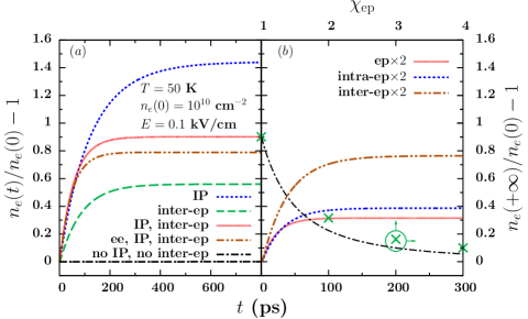
Figure 1: (Color online) Temporal evolution of $n_{e}(t)/n_{e}(0)-1$ with $E=0.1$ kV/cm, $T=50$ K and $n_{e}(0)=10^{10}$ cm^-2. During calculation, the electron-impurity scattering is not included while the intra-band electron-phonon scattering (labeled as intra-ep) is always present. (a): The chain curve is calculated without the inter-band precession (labeled as IP) and inter-band electron-phonon scattering (labeled as inter-ep), the dashed (dotted) one with only the inter-band electron-phonon scattering (inter-band precession), while the solid one with both the inter-band precession and inter-band electron-phonon scattering. The double-dotted chain curve is calculated with the inter-band precession, inter-band electron-phonon scattering and also the electron-electron Coulomb scattering (labeled as ee). (b): Temporal evolution of $n_{e}(t)/n_{e}(0)-1$ with the electron-phonon scattering artificially strengthened. The inter-band precession is always included. The solid curve is calculated with both the intra- and inter-band electron-phonon scatterings strengthened by a factor $\chi_{\rm ep}=2$, while the dotted (double-dotted chain) one with only the intra-band (inter-band) electron-phonon scattering strengthened by a factor 2. The crosses (with scales on the top and right-hand side of the frame) are the relative variation of $n_{e}$ reached in the steady state, $n_{e}(+\infty)/n_{e}(0)-1$, against the modulation factor $\chi_{\rm ep}$ ranging from 1 to 4. The chain curve (with scales on the top and right-hand side of the frame) is the function $[n_{e}(+\infty)/n_{e}(0)-1]|_{\chi_{\rm ep}=1}/\chi_{\rm ep}^{2}$.

We take an $n$-type degenerate case with $T=50$ K and $n_{e}(0)=10^{10}$ cm^-2 (the corresponding Fermi energy is $\varepsilon_{f}\approx 12$ meV and the Fermi momentum is $k_{f}\approx 0.035$ nm^-1) as an example to show the temporal evolution of the relative change of electron density in the conduction band, $n_{e}(t)/n_{e}(0)-1$, under electric field $E=0.1$ kV/cm. It is seen in Fig. 1(a) that when both the inter-band precession and inter-band electron-phonon scattering are excluded, $n_{e}(t)$ remains almost unchanged (chain curve). However, once the inter-band precession is included, electrons can be effectively transferred from the lower band to the higher one (dotted curve). The scenario is that, the electrons are precessed from the states below the Dirac point to the ones above and then driven away to higher-energy states by the electric field. The transfer of electrons can also be alternatively realized with the assistance of phonons (dashed curve). Around the Dirac point (with $k<k_{0}\equiv\omega_{0}/v_{f}\approx 0.022$ nm^-1), when electrons in the conduction band are driven away to higher-energy states, electrons in the valence band tend to enter the conduction band by absorbing phonons. However, the above two effects are not definitely superimposed when both of them are present. When the inter-band precession transfers electrons between two bands effectively, i.e., leads to substantial nonequilibrium between the two bands (such as the case presented here), electrons in the conduction band tend to fall back to the valence band by emitting phonons. Therefore, when both the inter-band scattering and inter-band precession are included, the steady-state electron density in the conduction band decreases compared to the case with only the inter-band precession (compare the solid and dotted curves).

As pointed out above, the inter-band precession and inter-band scattering open channels for electron transfer between the two bands. However, the steady state of the two-band system is determined by the balance between the rates of energy gain from electric field and the energy loss to phonons. The former is determined by $\partial_{t}\varepsilon_{i}(t)=E{\tilde{j}}_{x}(t)\propto E{\tilde{S}}_{y}(t)$ [refer to Eq. (7)]. If the steady state is not far away from the equilibrium, one approximately has $\partial_{t}\varepsilon_{i}(+\infty)\propto E^{2}|g_{0}|^{-2}$ in the presence of electron-phonon scattering only. The dominant channel of the energy loss is the intra-band electron-phonon scattering. That is because the inter-band electron-phonon scattering is limited to a small finite region $k<k_{0}$ in momentum space, and also, with such small momentum, the scattering is weak as the rate is $\propto k$. A rough estimation gives that the rate of energy loss due to the intra-band electron-phonon scattering for the degenerate case with both low temperature and electron density is $\partial_{t}\varepsilon_{o}(t)\propto|g_{0}|^{2}[n_{e}(t)-n_{e}(0)]$ (refer to Appendix B). Therefore in the steady state not far away from the equilibrium, one has

$$n_{e}(+\infty)-n_{e}(0)\propto E^{2}|g_{0}|^{-4},$$ (21)

required by $\partial_{t}\varepsilon_{i}(+\infty)=\partial_{t}\varepsilon_{o}(+\infty)$.

Based on Eq. (21), it is found that the strengthening of the electron-phonon scattering, especially the intra-band part, leads to the decrease in $n_{e}(+\infty)/n_{e}(0)-1$. In Fig. 1(b) we numerically verify this by performing similar calculation as in (a) but with the electron-phonon scattering artificially strengthened. It is shown by the solid curve that when the total electron-phonon scattering is strengthened by a factor $\chi_{\rm ep}=2$ (solid curve), $n_{e}(+\infty)/n_{e}(0)-1$ substantially decreases compared to the genuine case [solid curve in (a)]. When only either the intra- or inter-band electron-phonon scattering is strengthened (dotted and double-dotted chain curves, respectively), $n_{e}(+\infty)/n_{e}(0)-1$ also decreases. However, the decrease is not obvious when only the inter-band electron-phonon scattering is strengthened (double-dotted chain curve), indicating that the contribution to the energy loss by the inter-band electron-phonon scattering is indeed relatively weak. We further show the steady-state value, $n_{e}(+\infty)/n_{e}(0)-1$, against $\chi_{\rm ep}$ ranging from 1 to 4 by the crosses (the scales are on the top and right-hand side of the frame). It is seen that approximately $n_{e}(+\infty)/n_{e}(0)-1\propto\chi_{\rm ep}^{-2}$, satisfying Eq. (21) [as a guide to the eye, a function proportional to $\chi_{\rm ep}^{-2}$, $[n_{e}(+\infty)/n_{e}(0)-1]|_{\chi_{\rm ep}=1}/\chi_{\rm ep}^{2}$, is plotted by the chain curve in (b)].

At last we briefly address the effect of electron-impurity and electron-electron Coulomb scatterings on the redistribution of electrons. Although neither of them leads to energy loss directly, both of them can limit the charge current and hence the energy injection rate of the electric field. The effect of impurities on charge current is apparent, as also explicitly indicated here by the combination of Eqs. (19) and (7). The Coulomb scattering is usually deemed to preserve the charge current. This is indeed the case in semiconductors with parabolic energy spectrum where both momentum and current are conserved during the Coulomb scattering. However, here with linear energy spectrum, only the momentum but not the current is conserved during the Coulomb scattering. This particular feature also exists in graphene with linear dispersion as well.kashuba085415 In fact, the effect of the Coulomb scattering can be conjectured based on our analytical study, which indicates that ${\tilde{j}}_{x}\propto{\tilde{S}}_{y}\propto\tau_{k}$ [Eqs. (7) and (18)]. With the addition of the Coulomb scattering, the momentum scattering time $\tau_{k}$ is reduced and hence the charge current decreases. Consequently, with the inclusion of the electron-impurity and/or electron-electron Coulomb scattering, the current and hence the energy injection rate of electric field decreases, resulting in less obvious redistribution of electrons. Nevertheless, due to the large relative static dielectric constant, the effect of the electron-impurity and electron-electron Coulomb scatterings is expected to be weak except when the temperature is low. In Fig. 1(a), we add the double-dotted chain curve calculated with the Coulomb scattering included. In the absence of impurities and under low temperature, the contribution of the Coulomb scattering is visible, with which the variation in $n_{e}$ decreases compared to the Coulomb scattering-free case (solid curve there).

IV.2 Charge and spin transport

In the following, we systematically investigate the charge and spin transport under the electric field, first in the low electric field regime and then the large one.

IV.2.1 Low electric field regime

We first focus on the low electric field regime with $E\leq 0.1$ kV/cm and compare the numerical results with the analytical study in Sec. III. We consider three cases, (I) $n$-doped case with $T=50$ K and $n_{e}(0)=10^{10}$ cm^-2, (II) $n$-doped case with $T=300$ K and $n_{e}(0)=5\times 10^{11}$ cm^-2 and (III) intrinsic case with $T=300$ K and $\mu=0$ [correspondingly $n_{e}(0)\approx 0.8\times 10^{11}$ cm^-2]. Corresponding to these three cases, in Figs. 2(a)-(c), we show the dependence of $n_{e}(+\infty)/n_{e}(0)-1$ on the electric field with different impurity densities (note that the $y$-axes are in different scales in the three figures). For case (I) with low temperature $T=50$ K, $n_{e}$ increases obviously with the electric field, due to the small initial electron density in the conduction band $n_{e}(0)$ as well as the weak electron-phonon scattering. Moreover, $n_{e}$ increases with $E$ faster with a smaller impurity density as the electron-impurity scattering weakens. Besides, it is shown that when $E$ is small ($E<0.05$ kV/cm), $n_{e}(+\infty)/n_{e}(0)-1$ roughly exhibits a square dependence on $E$, consistent with Eq. (21). For case (II), which is highly degenerate and with strong electron-phonon scattering due to both high temperature and electron density, the electron density remains almost unchanged in the low electric field regime under investigation (the relative variation is of the order of $10^{-3}$). Nevertheless, for the intrinsic case (III), it becomes relatively easier for electrons to transfer due to the less occupancy of electrons in the conduction band, when compared to case (II). Finally, Figs. 2(b) and (c) show that the effect of impurities is negligible at $T=300$ K.

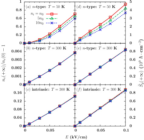
Figure 2: (Color online) (a)-(c): The relative change of electron density in the conduction band, $n_{e}(+\infty)/n_{e}(0)-1$, against the electric field $E$ for cases (I)-(III), respectively, with different impurity densities. $n_{0}=10^{10}$ cm^-2. (d)-(f): The induced spin polarization ${\tilde{S}}_{y}(+\infty)$ against the electric field $E$ for cases (I)-(III) with different impurity densities (the scale is on the right-hand side of the frame).

The induced spin polarizations in the steady state ${\tilde{S}}_{y}(+\infty)$ against the electric field $E$ for the three cases (I)-(III) are plotted in Figs. 2(d)-(f), respectively. It is shown that ${\tilde{S}}_{y}(+\infty)$ increases with $E$ much faster at 50 K than those at 300 K, mainly due to the weaker electron-phonon scattering. For case (I) with $T=50$ K, the electron-impurity scattering is important and $n_{e}$ increases with $E$ effectively [refer to Fig. 2(a)], therefore the rate of the increase in ${\tilde{S}}_{y}(+\infty)$ with $E$ shows impurity density dependence and also a slight electric field dependence [refer to Eq. (19)]. However, for cases (II) and (III) with $T=300$ K and hence the strong electron-phonon scattering, ${\tilde{S}}_{y}(+\infty)$ increases with $E$ linearly, with almost the identical rate under different impurity and electron densities. This is consistent with the analytical study: when the electron-phonon scattering dominates, the spin polarization increases with the electric field linearly in a rate solely determined by temperature [refer to Eq. (19) and the discussion there].

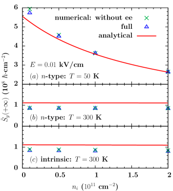
Figure 3: (Color online) Electric-field–induced spin polarization ${\tilde{S}}_{y}(+\infty)$ in the steady state against impurity density $n_{i}$ for cases (I)-(III), in (a)-(c) respectively. The triangles are obtained by numerically solving the full KSBEs, while the crosses are calculated without the electron-electron Coulomb scattering (labeled as ee). The solid curves are from the analytical result [Eq. (19)].

In the following, we compare the induced steady-state spin polarization numerically obtained to the analytical one at $E=0.01$ kV/cm, with which all the three cases (I)-(III) are close to the equilibrium. In Fig. 3, the impurity density dependence of the spin polarization from the numerical calculation with all the scatterings explicitly included is shown by triangles for the three cases. We also plot the numerical results without the Coulomb scattering by crosses. It is shown that the effect of the Coulomb scattering can only be visible when the impurity density approaches zero and the temperature is low. For comparison, the analytical calculation based on Eq. (19) is plotted by the solid curves in the figure. One finds that the analytical formula primarily captures the numerical results. We point out that at 300 K where the elastic scattering approximation for electron-phonon scattering is more reasonable ($k_{B}T\gg\hbar\omega_{0}$), the best fit to the numerical results by Eq. (19) requires $\alpha_{1}=17$. Finally, Figs. 3(b) and (c) indicate more clearly that at room temperature the electron-impurity scattering is negligible even when $n_{i}$ reaches $2\times 10^{11}$ cm^-2. In fact, according to the analytical study in Sec. III.1, the momentum scattering times are estimated to be $\tau_{k_{f}}^{\rm ei}=4.5$ ps and $\tau_{k_{f}}^{\rm ep}=2.5$ ps for case (I), $\tau_{k_{f}}^{\rm ei}=31.8$ ps and $\tau_{k_{f}}^{\rm ep}=0.07$ ps for case (II), and $\langle\tau_{k}^{\rm ei}\rangle=19.7$ ps and $\langle\tau_{k}^{\rm ep}\rangle=0.17$ ps for case (III) (in the estimation the impurity density is set as $n_{i}=10^{11}$ cm^-2). These values quantitatively support the dominance of the electron-phonon scattering at high temperature.

IV.2.2 Large electric field regime

After investigating the low field regime and comparing with the analytical study, we proceed with the large electric field regime ($E$ is upto 7 kV/cm). Both the intrinsic nondegenerate and $n$-type degenerate cases under 150 K and 300 K are considered. For the degenerate case, we set $n_{e}(0)=5\times 10^{11}$ cm^-2. The impurity density is fixed at $n_{i}=10^{11}$ cm^-2, with which the electron-impurity scattering is in fact negligible under the temperature investigated.

We first present the electric field dependence of the steady-state electron density in the conduction band, $n_{e}(+\infty)$, for the intrinsic and $n$-type cases at different temperatures. Figure 4 indicates that $n_{e}(+\infty)$ increases with $E$ almost linearly for both cases, except in the low electric field region $E<2$ kV/cm for the degenerate situation where the Pauli blocking is important. In fact, a nearly linear increase of electron density in conduction band with electric field is also observed in intrinsic graphene when $E>0.01$ kV/cm.balev165432 It is also noted that here in the nearly linear regime, the rate of the increase in $n_{e}(+\infty)$ with $E$ is determined by temperature and is insensitive to the electron density. It is believed that this linear relation as well as the temperature dependent increasing rate are attributed to the dominant electron-phonon scattering with almost constant scattering matrix element. As a comparison, we recalculate the intrinsic case at 300 K by artificially setting $\lambda_{1}=0$ and $\lambda_{2}=20$ eV$\cdot$nm² in the electron-phonon scattering matrix element [Eq. (9)]. The result is shown in the figure by dots. It is seen that it deviates from the linear relation obviously. Finally, we also present the calculation without the electron-electron Coulomb scattering for the intrinsic case at 150 K by the closed squares. The comparison between the closed and open squares indicates that the influence of the Coulomb scattering is marginal when the electric field is low and relatively effective when the electric field is high.

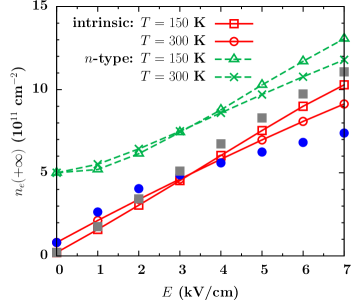
Figure 4: (Color online) Electric field dependence of the steady-state electron density in the conduction band $n_{e}(+\infty)$ for the intrinsic nondegenerate (solid curves) and $n$-type degenerate (dashed curves) cases under different temperatures. The dots are calculated for the intrinsic case at $T=300$ K by setting $\lambda_{1}=0$ and $\lambda_{2}=20$ eV$\cdot$nm² in the electron-phonon scattering matrix element [Eq. (9)]. The closed squares are calculated without the electron-electron Coulomb scattering for the intrinsic case at 150 K.

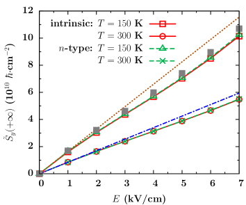
Figure 5: (Color online) Electric field dependence of induced spin polarization in the steady state for the intrinsic (solid curves) and $n$-type degenerate (dashed curves) cases at different temperatures. The dotted and chain curves are obtained from Eq. (19) with $\alpha_{1}=17$ at 150 K and 300 K, respectively. The closed squares are calculated without the electron-electron Coulomb scattering for the intrinsic case at 150 K.

We then look into the steady-state spin polarization ${\tilde{S}}_{y}(+\infty)$ induced by the electric field. In Fig. 5 the electric field dependence of ${\tilde{S}}_{y}(+\infty)$ for the intrinsic and $n$-type cases at different temperatures is plotted. Strikingly, in this whole large electric field region with the electron-phonon scattering being dominant, ${\tilde{S}}_{y}(+\infty)$ is solely determined by temperature, as previously revealed in the low electric field regime. Moreover, with the same electric field $E$, ${\tilde{S}}_{y}(+\infty)$ at 150 K is about 2 times as large as that at 300 K, approximately satisfying the analytical relation ${\tilde{S}}_{y}(+\infty)\propto T^{-1}$ at high temperature. In the figure we also plot the ${\tilde{S}}_{y}(+\infty)$-$E$ relation given by Eq. (19) (with modified $\alpha_{1}=17$) at 150 K (dotted curve) and 300 K (chain curve), respectively. It is seen that the analytical formula for ${\tilde{S}}_{y}(+\infty)$ can approximately apply up to $E_{c}=2$ kV/cm (4 kV/cm) at 150 K (300 K). When $E$ exceeds $E_{c}$, the electron heating becomes important. Therefore, with the occupation of larger-momentum states, the electron-phonon scattering is strengthened. At the same time, the momentum dependence of the electron-phonon scattering matrix element [arising from the term $\lambda_{2}q$ in Eq. (9)] also plays a role and further enhances the electron-phonon scattering. As a result, ${\tilde{S}}_{y}(+\infty)$ tends to decrease and hence deviates from the linear relation against $E$. Finally, the result obtained without the electron-electron Coulomb scattering for the intrinsic case at 150 K is also plotted by the closed squares. Again, the effect of the Coulomb scattering on spin polarization is also shown to be marginal, especially in the low electric field regime.

We now turn to study the mobility of the two-band system. According to Eq. (7), the steady-state charge current under the electric field is immediately obtained as ${\tilde{j}}_{x}(+\infty)=2ev_{f}{\tilde{S}}_{y}(+\infty)/\hbar$. Therefore, the steady-state mobility of the electron-hole system can be determined by $\mu_{c}={\tilde{j}}_{x}(+\infty)/[eE(n_{e}(+\infty)+n_{h}(+\infty))]$. In Fig. 6 we plot $\mu_{c}$ against $E$ for the intrinsic and $n$-type cases at different temperatures. It is shown that $\mu_{c}$ is around the order of $10^{3}$ cm²/(V$\cdot$s), in consistence with the experimental data.wei201402 ; kim459 ; analytis960 $\mu_{c}$ decreases with $E$ as electrons and holes are heated to occupy large-momentum states where strong electron-phonon scattering takes place. Moreover, with the increase of temperature from 150 to 300 K, $\mu_{c}$ decreases as well. In fact, we roughly have $\mu_{c}\approx({\mu_{c}^{0}}^{-1}+\gamma E)^{-1}$ as both $n_{e}(+\infty)+n_{h}(+\infty)$ and ${\tilde{j}}_{x}(+\infty)$ are close to linear functions of $E$. Here $\gamma$ is determined by the increasing rates of $n_{e}(+\infty)$ and ${\tilde{j}}_{x}(+\infty)$ with $E$, both of which are only sensitive to temperature when $E$ is large (as indicated by Figs. 4 and 5). Therefore, in the large electric field regime, $\mu_{c}\approx\gamma^{-1}E^{-1}$, with $\gamma$ determined by the temperature. This feature is manifested in Fig. 6 when $E\gtrsim 3$ kV/cm.

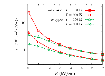
Figure 6: (Color online) Electric field dependence of mobility for the electron-hole system in the intrinsic (solid curves) and $n$-type (dashed curves) cases at different temperatures.

IV.3 Effect of the Coulomb scattering

Now we turn to see the effect of the Coulomb scattering on the steady state established in the presence of electric field. It has been revealed in the previous section that due to the large relative static dielectric constant, the influence of the Coulomb scattering is marginal in the presence of electron-phonon and electron-impurity scatterings. With the weak Coulomb scattering, electrons in two bands fail to reach the drifted Fermi distribution with a unified hot-electron temperature in the steady state. To reveal this, we take the intrinsic case with $T=300$ K and $E=3$ kV/cm as an example to plot the dependence of function ${\cal F}_{{\bf k}+}\equiv\log(1/f_{{\bf k}+}-1)$ on $k$ along the $x$-axis in Fig. 7, with different Coulomb scattering strengths adjusted artificially.yzhou The comparison among these sets of data indicates that only when the Coulomb scattering is strong enough (e.g., with the Coulomb scattering term rescaled by a factor $\chi_{\rm ee}=50$), in the steady state the drifted Fermi distribution $f_{{\bf k}\pm}=1/\{\exp[(\hbar v_{f}|{\bf k}-k_{x}^{0}|-\mu_{\pm})/(k_{B}T_{e})]+1\}$ is reached. Here $T_{e}$ is the unified hot-electron temperature and $k_{x}^{0}$ is the shift of the momentum center limited by the scattering. Both can be obtained from the slope of the wings of the “V” shape and the position of the valley, respectively (refer to the solid curve as a guide to the eye). $\mu_{\pm}$ are chemical potentials for the two bands. For the intrinsic case as presented here, $\mu_{+}=-\mu_{-}$, due to the symmetry between the two bands. In the inset of the figure we plot both ${\cal F}_{{\bf k}+}$ (closed circles) and ${\cal F}_{{\bf k}-}$ (open circles) for the genuine case (with $\chi_{\rm ee}=1$) in a small momentum scale. Although the drifted Fermi distribution is not established, the symmetry between the conduction and valence bands is clearly indicated by the inset.

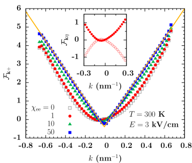
Figure 7: (Color online) Function ${\cal F}_{{\bf k}+}\equiv\log(1/f_{{\bf k}+}-1)$ against momentum $k$ along the $x$-axis in the steady state, evolving from the intrinsic case with $T=300$ K and $E=3$ kV/cm. The dots are obtained from the calculation for the genuine case, while the open squares, triangles and closed squares are from the calculation with the Coulomb scattering term multiplied by $\chi_{\rm ee}=0$, 10 and 50, respectively. The solid line is plotted as a guide to the eye by fitting the closed squares with hot-electron temperature $T_{e}\approx 488$ K. Inset: Function ${\cal F}_{{\bf k}\eta}\equiv\log(1/f_{{\bf k}\eta}-1)$ [closed (open) circles are for electrons in conduction (valence) band with $\eta=+$ ($-$)] against momentum $k$ along the $x$-axis in a small momentum scale in the steady state for the genuine case.

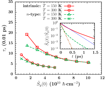
Figure 8: (Color online) Spin relaxation time $\tau_{s}$ against the initial spin polarization ${\tilde{S}}_{y}(0)$ for the intrinsic (solid curves) and $n$-type (dashed curves) cases at different temperatures. The temporal evolution of ${\tilde{S}}_{y}(t)/{\tilde{S}}_{y}(0)$ is plotted in the inset for two cases, with ${\tilde{S}}_{y}(0)$ initialized from the intrinsic situation at 150 K under electric field 1 (solid curve) and 7 kV/cm (dashed curve), respectively. The dotted (chain) curve is the exponential fit to the rapid decay in the beginning of the solid (dashed) curve.

IV.4 Spin relaxation

Finally, we start from the steady-state spin polarization reached previously under the electric field, to study the spin relaxation by turning off the electric field. The zero point of time, $t=0$, is reset to be the moment at which the electric field is turned off. Beginning at $t=0$, the heated electrons cool down to the original Fermi distribution in the time scale of energy relaxation, which is as long as $\sim$100-1000 ps, mainly due to the weak inter-band electron-phonon scattering. However, the spin polarization relaxes in the time scale of momentum scattering which is quite short.schwab67004 ; burkov066802 According to Eq. (20), ${\tilde{S}}_{ky}(t)$ relaxes approximately in the exponential form when $v_{f}k\tau_{k}\gg 1$. The total spin polarization ${\tilde{S}}_{y}(t)$, containing a summation of ${\tilde{S}}_{ky}(t)$ over momentum, does not definitely relax in a fine exponential form. Our calculation shows that ${\tilde{S}}_{y}(t)$ against $t$ decays first very fast to about $0.1{\tilde{S}}_{y}(0)$ but then slowly. The slowly-decaying tail with small magnitude is determined by the low-energy states near the Dirac point with long momentum relaxation times. As an example, in the inset of Fig. 8, we plot the dependence of ${\tilde{S}}_{y}(t)/{\tilde{S}}_{y}(0)$ against $t$ for two cases by the solid and dashed curves. In these two cases ${\tilde{S}}_{y}(0)$ are initialized from the intrinsic situation at 150 K under electric field 1 (solid curve) and 7 kV/cm (dashed curve), respectively. To obtain the spin relaxation time $\tau_{s}$, we fit the rapid decaying part in the beginning by an exponential function, as illustrated by the dotted and chain curves in the inset.

The spin relaxation time $\tau_{s}$ against the initial spin polarization ${\tilde{S}}_{y}(0)$ for the intrinsic and $n$-type cases at different temperatures is plotted in Fig. 8. It is shown that the spin relaxation time is of the order of 0.01-0.1 ps, mainly limited by the electron-phonon scattering. In fact, a momentum relaxation time of the similar order is given from both estimation and experiment by Butch et al..butch241301 The decrease of $\tau_{s}$ with the increase of ${\tilde{S}}_{y}(0)$ is due to the fact that the larger ${\tilde{S}}_{y}(0)$ is initialized by the higher electric field, with which the electrons and holes occupy larger-momentum states and hence exhibit faster momentum relaxation. Besides, with higher temperature, the spin relaxation time also decreases as the electron-phonon scattering is strengthened.

V Conclusion

In conclusion, we have studied the charge and spin transport under the influence of high electric field (up to several kV/cm) on the surface of topological insulator Bi₂Se₃, by means of the KSBEs. We assume that the Fermi level, adjustable by doping,analytis960 ; kulbachinskii15733 ; wei201402 ; xia398 ; hor195208 ; ren075316 is located in the bulk gap. Therefore the bulk states are excluded from our study. With moderate electron and hole densities, the surface state around the Dirac point can be depicted by the Rashba spin-orbit coupling. In our study, both the conduction and valence bands of the surface state are considered, with the inter-band coherence explicitly included. Apart from the driving effect in each band, due to the spin mixing of conduction and valence bands, the electric field also leads to inter-band precession. This differs from the semiconductors with parabolic energy spectrum.

In Bi₂Se₃, the relative static dielectric constant is as large as 100, indicating weak electron-impurity and electron-electron Coulomb scatterings. With the weak Coulomb scattering, electrons in the two bands fail to establish a drifted Fermi distribution with a unified hot-electron temperature under the driving of the electric field. The electron-surface optical phonon scattering dominates in a large temperature region. Moreover, the electron-phonon scattering matrix element is approximately constant due to its marginal dependence on momentum. This feature leads to particular properties of charge and spin transport on the surface of Bi₂Se₃.

Our study reveals that in the presence of driving of the electric field, both the inter-band precession and inter-band electron-phonon scattering cause electrons to transfer from the valence band to the conduction one. Due to the dominant electron-phonon scattering, the variation in electron density for each band is linear in the electric field when the latter is high, despite whether the initial state is degenerate or nondegenerate. It is also found that due to the spin-momentum locking from the Rashba spin-orbit coupling, a transverse spin polarization is induced by the electric field, with the magnitude proportional to the momentum scattering time. Besides, the spin polarization is linear in the electric field when the latter is small but deviates from the linear relation when the latter is large enough as the electron-phonon scattering is enhanced due to the heating of electrons. Moreover, a very interesting feature is that at high temperature, the spin polarization is inversely proportional to the temperature but insensitive to the electron density.

The cooling of hot carriers and the relaxation of spin polarization induced by the electric field are investigated by turning off the electric field after reaching the steady state. It is found that the hot carriers cool down in a time scale of energy relaxation, which is quite long and is of the order of 100-1000 ps. However, due to the spin-momentum locking again, the spin polarization relaxes in a time scale of momentum scattering. The spin polarization is mainly contributed by the states with large momentum. Therefore, it decays rapidly within the time of the order of 0.01-0.1 ps. Following this rapid decay, there is a slowly damping tail. This tail is attributed to the low-energy states near the Dirac point where the momentum scattering is weak.

Appendix A Scattering term in KSBEs

The scattering term in Eq. (2) can be written as

$$\partial_{t}\rho_{\bf k}(t)|_{\rm{scat}}= S_{\bf k}(>,<)-S_{\bf k}(<,>)+S_{\bf k}^{\dagger}(>,<)$$

$$-S_{\bf k}^{\dagger}(<,>),$$ (22)

with $S_{\bf k}(>,<)=S_{\bf k}^{\rm ep}(>,<)+S_{\bf k}^{\rm ei}(>,<)+S_{\bf k}^{\rm ee}(>,<)$ from the electron-surface optical phonon, electron-impurity and electron-electron scatterings, respectively. Here

$$S_{\bf k}^{\rm ep}(>,<)= \frac{\pi}{\hbar}\sum_{{\bf k}^{\prime}\eta_{1}\eta_{2}}|g_{{\bf k}-{\bf k}^{\prime}}|^{2}\Lambda_{{\bf k},{\bf k}^{\prime}}\rho_{{\bf k}^{\prime}}^{>}(t)T_{\eta_{1}}\Lambda_{{\bf k}^{\prime},{\bf k}}T_{\eta_{2}}\rho_{{\bf k}}^{<}(t)[N_{0}^{<}\delta(\varepsilon_{{\bf k}^{\prime}\eta_{1}}-\varepsilon_{{\bf k}\eta_{2}}-\hbar\omega_{0})+N_{0}^{>}\delta(\varepsilon_{{\bf k}^{\prime}\eta_{1}}-\varepsilon_{{\bf k}\eta_{2}}+\hbar\omega_{0})],$$ (23)

$$S_{\bf k}^{\rm ei}(>,<)= \frac{\pi n_{i}}{\hbar}\sum_{{\bf k}^{\prime}\eta_{1}\eta_{2}}|D_{{\bf k}-{\bf k}^{\prime}}|^{2}\Lambda_{{\bf k},{\bf k}^{\prime}}\rho_{{\bf k}^{\prime}}^{>}(t)T_{\eta_{1}}\Lambda_{{\bf k}^{\prime},{\bf k}}T_{\eta_{2}}\rho_{{\bf k}}^{<}(t)\delta(\varepsilon_{{\bf k}^{\prime}\eta_{1}}-\varepsilon_{{\bf k}\eta_{2}}),$$ (24)

$$S_{\bf k}^{\rm ee}(>,<)= \frac{\pi}{\hbar}\sum_{{\bf k}^{\prime}\eta_{1}\eta_{2}}\Lambda_{{\bf k},{\bf k}^{\prime}}\rho_{{\bf k}^{\prime}}^{>}(t)T_{\eta_{1}}\Lambda_{{\bf k}^{\prime},{\bf k}}T_{\eta_{2}}\rho_{{\bf k}}^{<}(t)\sum_{{\bf q}\eta_{3}-\eta_{6}}V_{{\bf k}-{\bf k}^{\prime}}^{r}(\varepsilon_{{\bf q}\eta_{3}}-\varepsilon_{{\bf q}+{\bf k}^{\prime}-{\bf k}\eta_{4}})V_{{\bf k}-{\bf k}^{\prime}}^{a}(\varepsilon_{{\bf q}\eta_{5}}-\varepsilon_{{\bf q}+{\bf k}^{\prime}-{\bf k}\eta_{6}})$$

$$\times\mbox{Tr}[\Lambda_{{\bf q},{\bf q}+{\bf k}^{\prime}-{\bf k}}T_{\eta_{6}}\rho_{{\bf q}+{\bf k}^{\prime}-{\bf k}}^{<}(t)T_{\eta_{4}}\Lambda_{{\bf q}+{\bf k}^{\prime}-{\bf k},{\bf q}}T_{\eta_{3}}\rho_{\bf q}^{>}(t)T_{\eta_{5}}]\delta(\varepsilon_{{\bf k}^{\prime}\eta_{1}}-\varepsilon_{{\bf k}\eta_{2}}+\varepsilon_{{\bf q}\eta_{5}}-\varepsilon_{{\bf q}+{\bf k}^{\prime}-{\bf k}\eta_{6}}).$$ (25)

To obtain the above equations, the Markovian approximation, $\rho^{I}_{\bf k}(t^{\prime})\approx\rho^{I}_{\bf k}(t)$, is adopted in the interaction picture. Here $\rho^{I}_{\bf k}(t)\equiv e^{iE_{\bf k}t}\rho_{\bf k}(t)e^{-iE_{\bf k}t}$ with the matrix $E_{\bf k}\equiv\mbox{diag}\{\varepsilon_{{\bf k}+},\varepsilon_{{\bf k}-}\}$. Equivalently, in the Schrödinger picture, the Markovian approximation is written as $\rho_{\bf k}(t^{\prime})\approx e^{-iE_{\bf k}(t^{\prime}-t)}\rho_{\bf k}(t)e^{iE_{\bf k}(t^{\prime}-t)}$. With this approximation, the scattering terms of KSBEswu-review are consistent with those of kinetic Bloch equations in semiconductors.haug However, in the work by Culcer et al., the Markovian approximation is mistakenly carried out as $\rho_{\bf k}(t^{\prime})\approx\rho_{\bf k}(t)$ in the Schrödinger picture.culcer155457 Therefore, the scattering term given there deviates from ours. In Eqs. (23)-(25), $\Lambda_{{\bf k},{\bf k}^{\prime}}=U_{\bf k}^{\dagger}U_{{\bf k}^{\prime}}$ [$U_{\bf k}$ is given in Eq. (5)] and $T_{\eta_{i}}=\frac{1}{2}(1+\eta_{i}\sigma_{z})$ with $\eta_{i}=\pm$. $\rho_{\bf k}^{<}(t)\equiv\rho_{\bf k}(t)$ and $\rho_{\bf k}^{>}(t)\equiv 1-\rho_{\bf k}(t)$. $N_{0}^{>}\equiv N_{0}+1$ and $N_{0}^{<}\equiv N_{0}$ where $N_{0}$ is the Boson distribution of surface optical phonons with energy $\hbar\omega_{0}=7.4$ meV.zhu186102 $|g_{\bf q}|^{2}$ is the electron-phonon scattering matrix element given by Eq. (9). $|D_{\bf q}|^{2}=|Z_{i}V_{q}^{0}e^{-qd}/\epsilon({\bf q},0)|^{2}$ is the electron-impurity scattering matrix element, where $Z_{i}$ is the charge number of impurity (assumed to be 1 here), $d$ is the effective distance of impurities from the surface two-dimensional electron layer (assumed to be zero following Culcer et al.culcer155457 ), and $V_{q}^{0}=2\pi\hbar v_{f}r_{s}/q$ with $r_{s}=e^{2}/(4\pi\epsilon_{0}\kappa_{0}\hbar v_{f})$. In Eq. (25), $V_{\bf q}^{r}(\hbar\omega)=V_{q}^{0}/\epsilon({\bf q},\omega)$ and $V_{\bf q}^{a}(\hbar\omega)={V_{\bf q}^{r}}^{\ast}(\hbar\omega)$ are the retarded and advanced Coulomb potentials with dynamic screening, respectively. The RPA screening $\epsilon({\bf q},\omega)=1-V_{q}^{0}\Pi({\bf q},\omega)$,hwang205418 ; ramezanali214015 ; culcer155457 with

$$\Pi({\bf q},\omega)= \sum_{{\bf k}\eta_{1}\eta_{2}}\frac{f_{{\bf k}\eta_{1}}-f_{{\bf k}+{\bf q}\eta_{2}}}{\hbar\omega+\varepsilon_{{\bf k}\eta_{1}}-\varepsilon_{{\bf k}+{\bf q}\eta_{2}}+i0^{+}}$$

$$\times[1+\eta_{1}\eta_{2}\cos(\theta_{\bf k}-\theta_{{\bf k}+{\bf q}})]/2.$$ (26)

In the $n$-type degenerate (intrinsic nondegenerate) situation, under the long-wavelength and static limit, $\Pi(0,0)=-k_{f}/(2\pi\hbar v_{f})$ (Ref. culcer155457, ) [$\Pi(0,0)=-k_{B}T\ln 4/(2\pi\hbar^{2}v_{f}^{2})$] given by Eq. (26) with $f_{{\bf k}\eta}$ substituted by the equilibrium Fermi distribution. Therefore $\epsilon(0,0)=1+q_{s}/q$ with $q_{s}=r_{s}k_{f}$ ($q_{s}=r_{s}k_{B}T\ln 4/\hbar v_{f}$) for the $n$-type degenerate (intrinsic nondegenerate) case. Especially, for the intrinsic case, due to the large Fermi velocity $v_{f}$ and small $r_{s}$, the screening is very weak and we further approximate $\epsilon(0,0)\approx 1$. These approximations for screening are utilized in analytically calculating the momentum relaxation time limited by the electron-impurity scattering in Sec. III.1.

Appendix B Energy loss rate due to the electron-phonon scattering

The energy loss rate, induced by the electron-phonon scattering solely, satisfies

$$\partial_{t}\varepsilon_{o}(t)=\sum_{\bf k}\hbar v_{f}k\mbox{Tr}[\sigma_{z}\partial_{t}\rho_{\bf k}(t)\big{|}_{\rm scat}^{\rm ep}].$$ (27)

Near the equilibrium, approximating $\rho_{\bf k}(t)$ isotropically and retaining its diagonal part only, one has

$$\partial_{t}\varepsilon_{o}(t) \approx\frac{|g_{0}|^{2}}{4\pi\hbar}\sum_{\eta=\pm}\Big{\{}k_{0}\int_{0}^{+\infty}dkk(k+k_{0})[N_{0}^{>}f_{k+k_{0}}^{\eta}(t)$$

$$-N_{0}^{<}f_{k}^{\eta}(t)-f_{k}^{\eta}(t)f_{k+k_{0}}^{\eta}(t)]+\int_{0}^{k_{0}}dkk^{2}(k_{0}-k)$$

$$\times[N_{0}^{<}(f_{k_{0}-k}^{\eta}(t)+f_{k}^{\eta}(t)-1)+f_{k_{0}-k}^{\eta}(t)f_{k}^{-\eta}(t)]\Big{\}}.$$ (28)

Here $f_{\bf k}^{+}(t)\equiv f_{{\bf k}+}(t)$ and $f_{\bf k}^{-}(t)\equiv 1-f_{{\bf k}-}(t)$ stand for electron and hole distributions in the conduction and valence bands, respectively. On the right-hand side of the equation, the first integral is contributed by the intra-band electron-phonon scattering in both bands while the second one by the inter-band electron-phonon scattering. For the $n$-type degenerate case with both low temperature and electron density, we take into account the contribution of the intra-conduction band electron-phonon scattering to calculate the energy loss rate as

$$\partial_{t}\varepsilon_{o}(t)\approx \frac{|g_{0}|^{2}k_{0}^{2}}{4\pi\hbar}\int_{0}^{+\infty}dkk[N_{0}^{>}f_{k+k_{0}}^{+}(t)-N_{0}^{<}f_{k}^{+}(t)$$

$$-f_{k}^{+}(t)f_{k+k_{0}}^{+}(t)].$$ (29)

By using the detailed balance condition satisfied in the initial equilibrium state, $N_{0}^{>}f^{+}_{k+k_{0}}(0)-N_{0}^{<}f_{k}^{+}(0)-f_{k}^{+}(0)f_{k+k_{0}}^{+}(0)=0$, one has

$$\partial_{t}\varepsilon_{o}(t)\approx \frac{|g_{0}|^{2}k_{0}^{2}}{4\pi\hbar}\int_{0}^{+\infty}dkk\Big{\{}N_{0}^{>}[f_{k+k_{0}}^{+}(t)-f_{k+k_{0}}^{+}(0)]$$

$$-N_{0}^{<}[f_{k}^{+}(t)-f_{k}^{+}(0)]-f_{k}^{+}(t)f_{k+k_{0}}^{+}(t)$$

$$+f_{k}^{+}(0)f_{k+k_{0}}^{+}(0)\Big{\}}$$

$$\approx \frac{|g_{0}|^{2}k_{0}^{2}}{4\pi\hbar}\int_{0}^{+\infty}dkk[f_{k}^{+}(t)-f_{k}^{+}(0)]$$

$$= \frac{|g_{0}|^{2}k_{0}^{2}}{2\hbar}[n_{e}(t)-n_{e}(0)].$$ (30)

This relation is utilized to obtain Eq. (21).

References

- (1) L. Fu, C. L. Kane, and E. J. Mele, Phys. Rev. Lett. 98, 106803 (2007).
- (2) H. J. Zhang, C. X. Liu, X. L. Qi, X. Dai, Z. Fang, and S. C. Zhang, Nat. Phys. 5, 438 (2009).
- (3) Y. Xia, D. Qian, D. Hsieh, L. Wray, A. Pal, H. Lin, A. Bansil, D. Grauer, R. J. Cava, and M. Z. Hasan, Nat. Phys. 5, 398 (2009).
- (4) Y. L. Chen, J. G. Analytis, J. H. Chu, Z. K. Liu, S. K. Mo, X. L. Qi, H. J. Zhang, D. H. Lu, X. Dai, Z. Fang, S. C. Zhang, I. R. Fisher, Z. Hussain, and Z. X. Shen, Science 325, 178 (2009).
- (5) D. Hsieh, Y. Xia, D. Qian, L. Wray, F. Meier, J. H. Dil, J. Osterwalder, L. Patthey, A. V. Fedorov, H. Lin, A. Bansil, D. Grauer, Y. S. Hor, R. J. Cava, and M. Z. Hasan, Phys. Rev. Lett. 103, 146401 (2009).
- (6) D. Hsieh, Y. Xia, D. Qian, L. Wray, J. H. Dil, F. Meier, J. Osterwalder, L. Patthey, J. G. Checkelsky, N. P. Ong, A. V. Fedorov, H. Lin, A. Bansil, D. Grauer, Y. S. Hor, R. J. Cava, and M. Z. Hasan, Nature 460, 1101 (2009).
- (7) M. Z. Hasan and C. L. Kane, Rev. Mod. Phys. 82, 3045 (2010).
- (8) J. G. Analytis, R. D. McDonald, S. C. Riggs, J. H. Chu, G. S. Boebinger, and I. R. Fisher, Nat. Phys. 6, 960 (2010).
- (9) X. L. Qi and S. C. Zhang, Rev. Mod. Phys. 83, 1057 (2011).
- (10) M. Z. Hasan and J. E. Moore, Ann. Rev. Cond. Matt. Phys. 2, 55 (2011).
- (11) H. Beidenkopf, P. Roushan, J. Seo, L. Gorman, I. Drozdov, Y. SanHor, R. J. Cava, and A. Yazdani, Nat. Phys. 7, 939 (2011).
- (12) D. Culcer, Physica E 44, 860 (2012).
- (13) G. A. Fiete, V. Chua, M. Kargarian, R. Lundgren, A. Rüegg, J. Wen, and V. Zyuzin, Physica E 44, 845 (2012).
- (14) D. Kim, S. Cho. N. P. Butch, P. Syers, K. Kirshenbaum, S. Adam, J. Paglione, and M. S. Fuhrer, Nat. Phys. 8, 459 (2012).
- (15) S. S. Hong, J. J. Cha, D. Kong, and Y. Cui, Nat. Commun. 3, 757 (2012).
- (16) G. Tkachov and E. M. Hankiewicz, arXiv:1208.1466.
- (17) X. L. Qi, T. L. Hughes, and S. C. Zhang, Phys. Rev. B 78, 195424 (2008).
- (18) J. E. Moore and L. Balents, Phys. Rev. B 75, 121306 (2007).
- (19) Y. A. Bychkov and E. I. Rashba, J. Phys. C 17, 6039 (1984).
- (20) C. X. Liu, X. L. Qi, H. J. Zhang, X. Dai, Z. Fang, and S. C. Zhang, Phys. Rev. B 82, 045122 (2010).
- (21) L. Fu, Phys. Rev. Lett. 103, 266801 (2009).
- (22) Z. H. Pan, E. Vescovo, A. V. Fedorov, D. Gardner, Y. S. Lee, S. Chu, G. D. Gu, and T. Valla, Phys. Rev. Lett. 106, 257004 (2011).
- (23) C. O. Aristizabal, M. S. Fuhrer, N. P. Butch, J. Paglione, and I. Appelbaum, Appl. Phys. Lett. 101, 023102 (2012).
- (24) D. Culcer, E. H. Hwang, T. D. Stanescu, and S. D. Sarma, Phys. Rev. B 82, 155457 (2010).
- (25) P. Schwab, R. Raimondi, and C. Gorini, Europhys. Lett. 93, 67004 (2011).
- (26) A. A. Burkov and D. G. Hawthorn, Phys. Rev. Lett. 105, 066802 (2010).
- (27) X. Zhu, L. Santos, R. Sankar, S. Chikara, C. Howard, F. C. Chou, C. Chamon, and M. E. Batanouny, Phys. Rev. Lett. 107, 186102 (2011).
- (28) E. M. Conwell, High Field Transport in Semiconductors (Pergamon, Oxford, 1972).
- (29) M. Q. Weng, M. W. Wu, and L. Jiang, Phys. Rev. B 69, 245320 (2004).
- (30) M. W. Wu, J. H. Jiang, and M. Q. Weng, Phys. Rep. 493, 61 (2010).
- (31) J. L. Cheng and M. W. Wu, J. Appl. Phys. 99, 083704 (2006).
- (32) Y. S. Hor, A. Richardella, P. Roushan, Y. Xia, J. G. Checkelsky, A. Yazdani, M. Z. Hasan, N. P. Ong, and R. J. Cava, Phys. Rev. B 79, 195208 (2009).
- (33) P. Wei, Z. Wang, X. Liu, V. Aji, and J. Shi, Phys. Rev. B 85, 201402(R) (2012).
- (34) V. A. Kulbachinskii, N. Miura, H. Nakagawa, H. Arimoto, T. Ikaida, P. Lostak, and C. Drasar, Phys. Rev. B 59, 15733 (1999).
- (35) Z. Ren, A. A. Taskin, S. Sasaki, K. Segawa, and Y. Ando, Phys. Rev. B 84, 075316 (2011).
- (36) W. Richter, H. Köhler, and C. R. Becker, Phys. Status Solidi B 84, 619 (1977).
- (37) N. P. Butch, K. Kirshenbaum, P. Syers, A. B. Sushkov, G. S. Jenkins, H. D. Drew, and J. Paglione, Phys. Rev. B 81, 241301 (2010).
- (38) O. G. Balev, F. T. Vasko, and V. Ryzhii, Phys. Rev. B 79, 165432 (2009).
- (39) S. Giraud and R. Egger, Phys. Rev. B 83, 245322 (2011).
- (40) R. C. Hatch, M. Bianchi, D. Guan, S. Bao, J. Mi, B. B. Iversen, L. Nilsson, L. Hornekær, and P. Hofmann, Phys. Rev. B 83, 241303 (2011).
- (41) T. Winzer, A. Knorr, and E. Malic, Nano Lett. 10, 4839 (2010).
- (42) T. Winzer and E. Malic, Phys. Rev. B 85, 241404(R) (2012).
- (43) E. H. Hwang and S. Das Sarma, Phys. Rev. B 75, 205418 (2007).
- (44) M. R. Ramezanali, M. M. Vazifeh, R. Asgari, M. Polini, and A. H. MacDonald, J. Phys. A: Math. Theor. 42, 214015 (2009).
- (45) Y. Zhou and M. W. Wu, Phys. Rev. B 82, 085304 (2010).
- (46) B. Y. Sun, Y. Zhou, and M. W. Wu, Phys. Rev. B 85, 125413 (2012).
- (47) A. B. Kashuba, Phys. Rev. B 78, 085415 (2008).
- (48) H. Haug and A. P. Jauho, Quantum kinetics in Transport and Optics of Semiconductors (Springer, Berlin, 1998).