20.5cm28cm

Locally symmetric submanifolds lift to spectral manifolds

Abstract. In this work we prove that every locally symmetric smooth submanifold $\mathcal{M}$ of $\mathbf{R}^{n}$ gives rise to a naturally defined smooth submanifold of the space of $n\times n$ symmetric matrices, called spectral manifold, consisting of all matrices whose ordered vector of eigenvalues belongs to $\mathcal{M}$. We also present an explicit formula for the dimension of the spectral manifold in terms of the dimension and the intrinsic properties of $\mathcal{M}$.

Key words. Locally symmetric set, spectral manifold, permutation, symmetric matrix, eigenvalue.

AMS Subject Classification. Primary 15A18, 53B25 Secondary 47A45, 05A05.

1 Introduction

Denoting by ${\bf S}^{n}$ the Euclidean space of $n\times n$ symmetric matrices with inner product $\langle X,Y\rangle=\mathrm{tr\,}(XY)$, we consider the spectral mapping $\lambda$, that is, a function from the space ${\bf S}^{n}$ to $\mathbf{R}^{n}$, which associates to $X\in{\bf S}^{n}$ the vector $\lambda(X)$ of its eigenvalues. More precisely, for a matrix $X\in{\bf S}^{n}$, the vector $\lambda(X)=(\lambda_{1}(X),\ldots,\lambda_{n}(X))$ consists of the eigenvalues of $X$ counted with multiplicities and ordered in a non-increasing way:

$$\lambda_{1}(X)\geq\lambda_{2}(X)\geq\cdots\geq\lambda_{n}(X).$$

The object of study in this paper are spectral sets, that is, subsets of ${\bf S}^{n}$ stable under orthogonal similarity transformations: a subset ${\bf M}\subset{\bf S}^{n}$ is a spectral set if for all $X\in{\bf M}$ and $U\in{\bf O}^{n}$ we have ${U}^{\!\top}XU\in{\bf M}$, where ${\bf O}^{n}$ is the set of $n\times n$ orthogonal matrices. In other words, if a matrix $X$ lies in a spectral set ${\bf M}\subset{\bf S}^{n}$, then so does its orbit under the natural action of the group of ${\bf O}^{n}$

$${\bf O}^{n}.X=\{{U}^{\!\top}XU:\ U\in{\bf O}^{n}\}.$$

The spectral sets are entirely defined by their eigenvalues, and can be equivalently defined as inverse images of subsets of $\mathbf{R}^{n}$ by the spectral mapping $\lambda$, that is,

$$\lambda^{-1}(M):=\{X\in{\bf S}^{n}:\lambda(X)\in M\},\quad\text{for some }\,M\subset\mathbf{R}^{n}.$$

For example, if $M$ is the Euclidean unit ball $B(0,1)$ of $\mathbf{R}^{n}$, then $\lambda^{-1}(M)$ is the Euclidean unit ball of ${\bf S}^{n}$ as well. A spectral set can be written as union of orbits:

$$\lambda^{-1}(M)=\bigcup_{x\in M}{\bf O}^{n}.\mathrm{Diag}(x),$$ (1.1)

where $\mathrm{Diag}(x)$ denotes the diagonal matrix with the vector $x\in\mathbf{R}^{n}$ on the main diagonal.

In this context, a general question arises: What properties on $M$ remain true on the corresponding spectral set $\lambda^{-1}(M)$?

In the sequel we often refer to this as the transfer principle. The spectral mapping $\lambda$ has nice geometrical properties, but it may behave very badly as far as, for example, differentiability is concerned. This imposes intrinsic difficulties for the formulation of a generic transfer principle. Invariance properties of $M$ under permutations often correct such bad behavior and allow us to deduce transfer properties between the sets $M$ and $\lambda^{-1}(M)$. A set $M\subset\mathbf{R}^{n}$ is symmetric if $\sigma M=M$ for all permutations $\sigma$ on $n$ elements, where the permutation $\sigma$ permutes the coordinates of vectors in $\mathbf{R}^{n}$ in the natural way. Thus, if the set $M\subset\mathbf{R}^{n}$ is symmetric, then properties such as closedness and convexity are transferred between $M$ and $\lambda^{-1}(M)$. Namely, $M$ is closed (respectively, convex [9], prox-regular [3]) if and only if $\lambda^{-1}(M)$ is closed (respectively, convex, prox-regular). The next result is another interesting example of such a transfer.

Proposition 1.1 (Transferring algebraicity).

Let $\mathcal{M}\subset\mathbf{R}^{n}$ be a symmetric algebraic variety. Then, $\lambda^{-1}(\mathcal{M})$ is an algebraic variety of ${\bf S}^{n}$.

Proof.  Let $p$ be any polynomial equation of $\mathcal{M}$, that is $p(x)=0$ if and only if $x\in\mathcal{M}$. Define the symmetric polynomial $q(x):=\sum_{\sigma}p^{2}(\sigma x)$. Notice that $q$ is again a polynomial equation of $\mathcal{M}$ and $q(\lambda(X))$ is an equation of $\lambda^{-1}(\mathcal{M})$. We just have to prove that $q\circ\lambda$ is a polynomial in the entries of $X$. It is known that $q$ can be written as a polynomial of the elementary symmetric polynomials $p_{1},p_{2},\ldots,p_{n}$. Each $p_{j}(\lambda(X))$, up to a sign, is a coefficient of the characteristic polynomial of $X$, thus it is a polynomial in $X$. Thus we can complete the proof.     

Concurrently, similar transfer properties hold for spectral functions, that is, functions $F\colon{\bf S}^{n}\rightarrow\mathbf{R}^{n}$ which are constant on the orbits ${\bf O}^{n}.X$ or equivalently, functions $F$ that can be written as $F=f\circ\lambda$ with $f\colon\mathbf{R}^{n}\rightarrow\mathbf{R}$ being symmetric, that is invariant under any permutation of entries of $x$. Since $f$ is symmetric, closedness and convexity are transferred between $f$ and $F$ (see [9] for details). More surprisingly, some differentiability properties are also transferred (see [8], [10] and [13]). As established recently in [3], the same happens for an important property of variational analysis, the so-called prox-regularity (we refer to [12] for the definition).

In this work, we study the transfer of differentiable structure of a submanifold $\mathcal{M}$ of $\mathbf{R}^{n}$ to the corresponding spectral set. This gives rise to an orbit-closed set $\lambda^{-1}(\mathcal{M})$ of ${\bf S}^{n}$, which, in case it is a manifold, will be called spectral manifold. Such spectral manifolds often appear in engineering sciences, often as constraints in feasibility problems (for example, in the design of tight frames [14] in image processing or in the design of low-rank controller [11] in control). Given a manifold $\mathcal{M}$, the answer, however, to the question of whether or not the spectral set $\lambda^{-1}(\mathcal{M})$ is a manifold of ${\bf S}^{n}$ is not direct: indeed, a careful glance at (1.1) reveals that ${\bf O}^{n}.\mathrm{Diag}(x)$ has a natural (quotient) manifold structure (we detail this in Section 3.1), but the question is how the different strata combine as $x$ moves along $\mathcal{M}$.

For functions, transferring local properties as differentiability requires some symmetry, albeit not with respect to all permutations: it turns out that many properties still hold under local symmetry, that is, invariance under permutations that preserve balls centered at the point of interest. We define precisely these permutations in Section 2.1, and we state in Theorem 3.2 that the differentiability of spectral functions is valid under this local invariance.

The main goal here is to prove that local smoothness of $\mathcal{M}$ is transferred to the spectral set $\lambda^{-1}(\mathcal{M})$, whenever $\mathcal{M}$ is locally symmetric. More precisely, our aim here is

• to prove that every connected $C^{k}$ locally symmetric manifold $\mathcal{M}$ of $\mathbb{R}^{n}$ is lifted to a connected $C^{k}$ manifold $\lambda^{-1}(\mathcal{M})$ of ${\bf S}^{n}$, for $k\in\{2,\infty,\omega\}$;

• to derive a formula for the dimension of $\lambda^{-1}(\mathcal{M})$ in terms of the dimension of $\mathcal{M}$ and some characteristic properties of $\mathcal{M}$.

This is eventually accomplished with Theorem 4.21. To get this result, we use extensively differential properties of spectral functions and geometric properties of locally symmetric manifolds. Roughly speaking, given a manifold $\mathcal{M}$ which is locally symmetric around $\bar{x}$, the idea of the proof is:

1. to exhibit a simple locally symmetric affine manifold $\mathcal{D}$, see (4.12), which will be used as a domain for a locally symmetric local equation for the manifold $\mathcal{M}$ around $\bar{x}$ (Theorem 4.12);

2. to show that $\lambda^{-1}(\mathcal{D})$ is a smooth manifold (Theorem 4.16) and use it as a domain for a local equation of $\lambda^{-1}(\mathcal{M})$ (see definition in (4.16)), in order to establish that the latter is a manifold (Theorem 4.21).

The paper is organized as follows. We start with grinding our tools: in Section 2 we recall basic properties of permutations and define a stratification of $\mathbf{R}^{n}$ naturally associated to them which will be used to study properties of locally symmetric manifolds in Section 3. Then, in Section 4 we establish the transfer of the differentiable structure from locally symmetric subsets of $\mathbf{R}^{n}$ to spectral sets of ${\bf S}^{n}$.

2 Preliminaries on permutations

This section gathers several basic results about permutations that are used extensively later. In particular, after defining order relations on the group of permutations in Subsection 2.1 and the associated stratification of $\mathbf{R}^{n}$ in Subsection 2.2, we introduce the subgroup of permutations that preserve balls centered at a given point.

2.1 Permutations and partitions

Denote by $\Sigma^{n}$ the group of permutations over $\mathbb{N}_{n}:=\{1,\ldots,n\}$. This group has a natural action on $\mathbf{R}^{n}$ defined for $x=(x_{1},\ldots,x_{n})$ by

$$\sigma x:=(x_{\sigma^{-1}(1)},\ldots,x_{\sigma^{-1}(n)}).$$ (2.1)

Given a permutation $\sigma\in\Sigma^{n}$, we define its support $\mathrm{supp}(\sigma)\subset\mathrm{N}_{n}$ as the set of indices $i\in\mathbb{N}_{n}$ that do not remain fixed under $\sigma$. Further, we denote by $\mathbf{R}^{n}_{\geq}$ the closed convex cone of all vectors $x\in\mathbf{R}^{n}$ with $x_{1}\geq x_{2}\geq\cdots\geq x_{n}$.

Before we proceed, let us recall some basic facts on permutations. A cycle of length $k\in\mathbb{N}_{n}$ is a permutation $\sigma\in\Sigma^{n}$ such that for $k$ distinct elements $i_{1},\ldots,i_{k}$ in $\mathbb{N}_{n}$ we have $\mathrm{supp}(\sigma)=\{i_{1},\ldots,i_{k}\},$ and $\sigma(i_{j})=i_{j+1\;(\operatorname{mod}\;k)}$; we represent $\sigma$ by $(i_{1},\ldots,i_{k})$. Every permutation has a cyclic decomposition: that is, every permutation $\sigma\in\Sigma^{n}$ can be represented (in a unique way up to reordering) as a composition of disjoint cycles

$$\sigma=\sigma_{1}\circ\cdots\circ\sigma_{m},\qquad\textrm{where the $\sigma_{i}$'s are cycles.}$$

It is easy to see that if the cycle decomposition of $\sigma\in\Sigma^{n}$ is

$$(a_{1},a_{2},\ldots,a_{k_{1}})(b_{1},b_{2},\ldots,b_{k_{2}})\cdots$$

then for any $\tau\in\Sigma^{n}$ the cycle decomposition of $\tau\sigma\tau^{-1}$ is

$$(\tau(a_{1}),\tau(a_{2}),\ldots,\tau(a_{k_{1}}))(\tau(b_{1}),\tau(b_{2}),\ldots,\tau(b_{k_{2}}))\cdots$$ (2.2)

Thus, the support $\mathrm{supp}(\sigma)$ of the permutation $\sigma$ is the (disjoint) union of the supports $I_{i}=\mathrm{supp}(\sigma_{i})$ of the cycles $\sigma_{i}$ of length at least two (the non-trivial cycles) in its cycle decomposition. The partition

$$\{I_{1},\ldots,I_{m},\mathbb{N}_{n}\setminus\mathrm{supp}(\sigma)\}$$

of $\mathbb{N}_{n}$ is thus naturally associated to the permutation $\sigma$. Splitting further the set $\mathbb{N}_{n}\setminus\mathrm{supp}(\sigma)$ into the singleton sets $\{j\}$ we obtain a refined partition of $\mathbb{N}_{n}$

$$P(\sigma):=\{I_{1},\ldots,I_{\kappa+m}\},$$ (2.3)

where $\kappa$ is the cardinality of the complement of the support of $\sigma$ in $\mathbb{N}_{n}$, and $m$ is the number of non-trivial cycles in the cyclic decomposition of $\sigma$. For example, for $\sigma=(123)(4)(5)\in\Sigma^{5}$ we have $\kappa=2$, $m=1$ and the partition of $\{\{1,2,3\},\{4\},\{5\}\}$ of $\mathbb{N}_{5}$. Thus, we obtain a correspondence from the set of permutations $\Sigma^{n}$ onto the set of partitions of $\mathbb{N}_{n}$.

Definition 2.1.

An order on the partitions:

Given two partitions $P$ and $P^{\prime}$ of $\mathbb{N}_{n}$ we say that $P^{\prime}$ is a refinement of $P$, written $P\subseteq P^{\prime}$, if every set in $P$ is a (disjoint) union of sets from $P^{\prime}$. If $P^{\prime}$ is a refinement of $P$ but $P$ is not a refinement of $P^{\prime}$ then we say that the refinement is strict and we write $P\subset P^{\prime}$. Observe this partial order is a lattice.

An order on the permutations:

The permutation $\sigma^{\prime}$ is said to be larger than or equivalent to $\sigma$, written $\sigma\precsim\sigma^{\prime}$, if $P(\sigma)\subseteq P(\sigma^{\prime})$. The permutation $\sigma^{\prime}$ is said to be strictly larger than $\sigma$, written $\sigma\prec\sigma^{\prime}$, if $P(\sigma)\subset P(\sigma^{\prime})$.

Equivalence in $\Sigma^{n}$:

The permutations $\sigma,\sigma^{\prime}\in\Sigma^{n}$ are said to be equivalent, written $\sigma\sim\sigma^{\prime}$, if they define the same partitions, that is if $P(\sigma)=P(\sigma^{\prime})$.

Block-Size type of a permutation:

Two permutations $\sigma$, $\sigma^{\prime}$ in $\Sigma^{n}$ are said to be of the same block-size type, whenever the set of cardinalities, counting repetitions, of the sets in the partitions $P(\sigma)$ and $P(\sigma^{\prime})$, see (2.3), are in a one-to-one correspondence. Notice that if $\sigma$ and $\sigma^{\prime}$ are of the same block-size type, then they are either equivalent or non-comparable.

We give illustrations (by means of simple examples) of the above notions, which are going to be used extensively in the paper.

Example 2.2 (Permutations vs Partitions).

The following simple examples illustrate the notions defined in Definition 2.1.

• The set of permutations of $\Sigma^{3}$ that are larger than or equivalent to $\sigma:=(1,2,3)$ is

  $$\{(1,2,3),(1,3,2),(1,2),(1,3),(2,3),\mbox{\rm id}_{3}\}.$$

• The following three permutations of $\Sigma^{4}$ have the same block-size type:

  $$\sigma=(123)(4),\quad\sigma^{\prime}=(132)(4),\quad\sigma^{\prime\prime}=(124)(3)\,.$$

  Note that the first two permutations are equivalent and not comparable to the third one.

• The minimal elements of $\Sigma^{n}$ under the partial order relation $\precsim$ are exactly the $n$-cycles, corresponding to the partition $\{\mathbb{N}_{n}\}$.

• The (unique) maximum element of $\Sigma^{n}$ under $\precsim$ is the identity permutation $\mathrm{id}_{n}$, corresponding to the discrete partition $\{\{i\}:i\in\mathbb{N}_{n}\}$.     

Consider two permutations $\sigma,\sigma^{\prime}\in\Sigma^{n}$ such that $\sigma^{\prime}\precsim\sigma$; according to the above, each cycle of $\sigma^{\prime}$ is either a permutation of the elements of a cycle in $\sigma$ (giving rise to the same set in the corresponding partitions $P(\sigma)$ and $P(\sigma^{\prime})$) or it is formed by merging (and permuting) elements from several cycles of $\sigma$. If no cycle of $\sigma^{\prime}$ is of the latter type, then $\sigma$ and $\sigma^{\prime}$ define the same partition (thus they are equivalent), while on the contrary, $\sigma^{\prime}\prec\sigma$. Later, in Subsection 3.3, we will introduce a subtle refinement of the order relation $\prec$, which will be of crucial importance in our development.

We also introduce another partition of $\mathbb{N}_{n}$ depending on the point $x\in\mathbf{R}^{n}$ denoted $P(x)$ and defined by the indexes of the equal coordinates of $x$. More precisely, for $i,j\in\mathbb{N}_{n}$ we have:

$$i,j\mbox{ are in the same subset of }P(x)\leavevmode\nobreak\ \leavevmode\nobreak\ \Longleftrightarrow\leavevmode\nobreak\ \leavevmode\nobreak\ x_{i}=x_{j}.$$ (2.4)

This partition will appear frequently in the sequel, when we study subsets of $\mathbf{R}^{n}$ that are symmetric around $x$. For $\bar{x}\in\mathbb{R}^{n}$ and $\bar{\sigma}\in\Sigma^{n}$, we define two invariant sets

$$\mathrm{Fix\,}(\bar{\sigma}):=\{x\in\mathbb{R}^{n}:\bar{\sigma}x=x\}\qquad\text{and}\qquad\mathrm{Fix\,}(\bar{x}):=\{\sigma\in\Sigma^{n}:\sigma\bar{x}=\bar{x}\}.$$

Then, in view of (2.4) we have

$$\bar{\sigma}\in\mathrm{Fix\,}(\bar{x})\leavevmode\nobreak\ \leavevmode\nobreak\ \Longleftrightarrow\leavevmode\nobreak\ \leavevmode\nobreak\ \bar{x}\in\mathrm{Fix\,}(\bar{\sigma})\leavevmode\nobreak\ \leavevmode\nobreak\ \Longleftrightarrow\leavevmode\nobreak\ \leavevmode\nobreak\ P(\bar{x})\subseteq P(\bar{\sigma}).$$ (2.5)

2.2 Stratification induced by the permutation group

In this section, we introduce a stratification of $\mathbf{R}^{n}$ associated with the set of permutations $\Sigma^{n}$. In view of (2.5), associated to a permutation $\sigma$ is the subset $\Delta(\sigma)$ of $\mathbf{R}^{n}$ defined by

$$\Delta(\sigma):=\{x\in\mathbf{R}^{n}:\ P(\sigma)=P(x)\}.$$ (2.6)

For $\sigma\in\Sigma^{n}$ and $P(\sigma)=\{I_{1},\ldots,I_{m}\}$, we have the representation

$$\Delta(\sigma)=\{x\in\mathbf{R}^{n}:x_{i}=x_{j}\iff\exists\,k\in\mathbb{N}_{m}\mbox{ with }i,j\in I_{k}\}.$$

Obviously $\Delta(\sigma)$ is an affine manifold, not connected in general. Note also that its orthogonal and bi-orthogonal spaces have the following expressions, respectively,

$$\Delta(\sigma)^{\perp}=\Big{\{}x\in\mathbb{R}^{n}:\sum\limits_{j\in I_{i}}x_{j}=0,\text{ for }i\in\mathbb{N}_{m}\Big{\}},$$ (2.7)

$$\Delta(\sigma)^{\perp\perp}=\{x\in\mathbb{R}^{n}:x_{i}=x_{j}\mbox{ for any }i,j\in I_{k},\ k\in\mathbb{N}_{m}\}.$$ (2.8)

Note that $\Delta(\sigma)^{\perp\perp}=\overline{\Delta(\sigma)}$, where the latter set is the closure of $\Delta(\sigma)$. Thus, $\Delta(\sigma)^{\perp}$ is a vector space of dimension $n-m$ while $\Delta(\sigma)^{\perp\perp}$ is a vector space of dimension $m$. For example, $\Delta({\rm id}_{n})^{\bot}=\{0\}$ and $\Delta({\rm id}_{n})^{\bot\bot}=\mathbb{R}^{n}$. We show now, among other things, that $\{\Delta(\sigma):\sigma\in\Sigma^{n}\}$ is a stratification of $\mathbf{R}^{n}$, that is, a collection of disjoint smooth submanifolds of $\mathbf{R}^{n}$ with union $\mathbf{R}^{n}$ that fit together in a regular way. In this case, the submanifolds in the stratification are affine.

Figure 1: The affine stratification of $\mathbf{R}^{3}$

Proposition 2.3 (Properties of $\Delta(\sigma)$).

(i) Let $x\in\mathbb{R}^{n}$ and let $P$ be any partition of $\mathbb{N}_{n}$. Then, $P(x)\subseteq P$ if and only if there is a sequence $x_{n}\rightarrow x$ in $\mathbf{R}^{n}$ satisfying $P(x_{n})=P$ for all $n\in\mathbb{N}$.

(ii) Let $\sigma,\sigma^{\prime}\in\Sigma^{n}$. Then,

$$\sigma\precsim\sigma^{\prime}\Longleftrightarrow\Delta(\sigma)\subset\Delta(\sigma^{\prime})^{\bot\bot},$$ (2.9)

$$\sigma\sim\sigma^{\prime}\Longleftrightarrow\Delta(\sigma)\cap\Delta(\sigma^{\prime})\neq\emptyset\Longleftrightarrow\Delta(\sigma)=\Delta(\sigma^{\prime}).$$ (2.10)

(iii) For any $\sigma\in\Sigma^{n}$ we have

$$\Delta(\sigma)^{\bot\bot}=\bigcup_{\sigma^{\prime}\precsim\sigma}\Delta(\sigma^{\prime}).$$ (2.11)

(iv) Given $\sigma,\sigma^{\prime}\in\Sigma^{n}$ let $\sigma\wedge\sigma^{\prime}$ be any infimum of $\sigma$ and $\sigma^{\prime}$ $($notice this is unique modulo $\sim)$. Then

$$\Delta(\sigma)^{\bot\bot}\cap\Delta(\sigma^{\prime})^{\bot\bot}=\Delta(\sigma\wedge\sigma^{\prime})^{\bot\bot}.$$ (2.12)

(v) For any $\tau,\sigma\in\Sigma^{n}$ we have

$$\tau\Delta(\sigma)=\Delta(\tau\sigma\tau^{-1}).$$

Proof.  Assertion $(i)$ is straightforward. Assertion $(ii)$ follows from $(i)$, (2.5), (2.6) and (2.8). Assertion $(iii)$ is a direct consequence of $(i)$, $(ii)$ and (2.8).

To show assertion $(iv)$, let first $x\in\Delta(\sigma)^{\bot\bot}\cap\Delta(\sigma^{\prime})^{\bot\bot}$. Then, in view of $(iii)$, there exist $\tau_{1}\precsim\sigma$ and $\tau_{2}\precsim\sigma^{\prime}$ such that $x\in\Delta(\tau_{1})\cap\Delta(\tau_{2})$. Thus, by (2.10), $\tau_{1}\sim\tau_{2}$ and by (2.9) they are both smaller than or equivalent to $\sigma\wedge\sigma^{\prime}$. Thus, $x\in\Delta(\sigma\wedge\sigma^{\prime})^{\bot\bot}$ showing that $\Delta(\sigma)^{\bot\bot}\cap\Delta(\sigma^{\prime})^{\bot\bot}\subset\Delta(\sigma\wedge\sigma^{\prime})^{\bot\bot}$. Let now $x\in\Delta(\sigma\wedge\sigma^{\prime})^{\bot\bot}$. Then, for some $\tau\precsim\sigma\wedge\sigma^{\prime}$ we have $x\in\Delta(\tau)$. Since $\tau\precsim\sigma$ and $\tau\precsim\sigma^{\prime}$ the inverse inclusion follows from $(iii)$.

We finally prove $(v)$. We have that $x\in\tau\Delta(\sigma)$ if and only if $\tau^{-1}x\in\Delta(\sigma)$. This latter happens if and only if for all $i,j\in\mathbb{N}_{n}$ one has $(\tau^{-1}x)_{i}=(\tau^{-1}x)_{j}$ precisely when $i,j$ belong to the same cycle of $\sigma$. By (2.1), this is equivalent to $x_{\tau(i)}=x_{\tau(j)}$ precisely when $i,j$ are in the same cycle of $\sigma$ for all $i,j\in\mathbb{N}_{n}$. In view of (2.2), $i,j$ are in the same cycle of $\sigma$ if and only if $\tau(i)$, $\tau(j)$ are in the same cycle of $\tau\sigma\tau^{-1}$. This completes the proof.     

Corollary 2.4 (Stratification).

The collection $\{\Delta(\sigma):\sigma\in\Sigma^{n}\}$ is an affine stratification of $\mathbb{R}^{n}$.

Proof.  Clearly, each $\Delta(\sigma)$ is an affine submanifold of $\mathbf{R}^{n}$. By (2.10), for any $\sigma,\sigma^{\prime}\in\Sigma^{n}$, the sets $\Delta(\sigma)$ and $\Delta(\sigma^{\prime})$ are either disjoint or they coincide. Thus, the elements in the set $\{\Delta(\sigma):\sigma\in\Sigma^{n}\}$ are disjoint. By construction, the union of all $\Delta(\sigma)$’s equals $\mathbf{R}^{n}$. The frontier condition of the stratification follows from (2.8) and (2.11).     

We introduce an important set for our next development. Consider the set of permutations that are larger than, or equivalent to a given permutation $\sigma\in\Sigma^{n}$

$$S^{\succsim}(\sigma):=\{\sigma^{\prime}\in\Sigma^{n}:\sigma^{\prime}\succsim\sigma\}.$$

Notice that $S^{\succsim}(\sigma)$ is a subgroup of $\Sigma^{n}$, and that

$$|S^{\succsim}(\sigma)|=(|I_{1}|)!\cdots(|I_{m}|)!,$$ (2.13)

if $P(\sigma)=\{I_{1},\ldots,I_{m}\}$. Observe then that $\sigma\sim\sigma^{\prime}$ if and only if $S^{\succsim}(\sigma)=S^{\succsim}(\sigma^{\prime})$. So we also introduce the corresponding set for a point $x\in\mathbf{R}^{n}$

$$S^{\succsim}(x):=S^{\succsim}(\sigma)\qquad\textrm{for any $\sigma$ such that $x\in\Delta(\sigma)$}\,,$$ (2.14)

which is nothing else than the set $\mathrm{Fix\,}(x)$. The forthcoming result shows that the above permutations are the only ones preserving balls centered at $\bar{x}$.

Lemma 2.5 (Local invariance and ball preservation).

For any $\bar{x}\in\mathbf{R}^{n}$, we have the dichotomy:

1. $\sigma\in S^{\succsim}(\bar{x})\ \Longleftrightarrow\ \forall\delta>0:\ \sigma B(\bar{x},\delta)=B(\bar{x},\delta)$;

2. $\sigma\not\in S^{\succsim}(\bar{x})\ \Longleftrightarrow\ \exists\delta>0:\ \sigma B(\bar{x},\delta)\cap B(\bar{x},\delta)=\emptyset$.

Proof.  Observe that $\sigma\in S^{\succsim}(\bar{x})$ if and only if $P(\bar{x})\subseteq P(\sigma)$ if and only if $\Arrowvert\bar{x}-\sigma\bar{x}\Arrowvert=0$. So implication $\Leftarrow$ of $(i)$ follows by taking $\delta\rightarrow 0$. The implication $\Rightarrow$ of $(i)$ comes from the symmetry of the norm which yields for any $x\in\mathbf{R}^{n}$

$$\Arrowvert x-\bar{x}\Arrowvert=\Arrowvert\sigma x-\sigma\bar{x}\Arrowvert=\Arrowvert\sigma x-\bar{x}\Arrowvert.$$

To prove $(ii)$, we can just consider $\delta=\Arrowvert\bar{x}-\sigma\bar{x}\Arrowvert/3$ and note that $\delta>0$ whenever $\sigma\notin S^{\succsim}(\bar{x})$. Utilizing

$$\Arrowvert\bar{x}-\sigma x\Arrowvert\geq|\Arrowvert\bar{x}-\sigma\bar{x}\Arrowvert-\Arrowvert\sigma\bar{x}-\sigma x\Arrowvert|=\Arrowvert\bar{x}-\sigma\bar{x}\Arrowvert-\Arrowvert\bar{x}-x\Arrowvert\geq 2\delta$$

concludes the proof.     

In words, if the partition associated to $\sigma$ refines the partition of $\bar{x}$, then $\sigma$ preserves all the balls centered at $\bar{x}$; and this property characterizes those permutations. The next corollary goes a bit further by saying that the preservation of only one ball, with a sufficiently small radius, also characterizes $S^{\succsim}(\bar{x})$.

Corollary 2.6 (Invariance of one ball).

For every $\bar{x}\in\mathbf{R}^{n}$ there exists $r>0$ such that:

$$\sigma\in S^{\succsim}(\bar{x})\Longleftrightarrow\sigma B(\bar{x},r)=B(\bar{x},r)\qquad\text{and}\qquad\sigma\not\in S^{\succsim}(\bar{x})\Longleftrightarrow\sigma B(\bar{x},r)\cap B(\bar{x},r)=\emptyset.$$

Proof.  For any $\sigma\notin S^{\succsim}(\bar{x})$, Lemma 2.5$(ii)$ gives a radius, that we denote here by $\delta_{\sigma}>0$, such that $\sigma B(\bar{x},\delta_{\sigma})\cap B(\bar{x},\delta_{\sigma})=\emptyset$. Note also that for all $\delta\leq\delta_{\sigma}$, there still holds $\sigma B(\bar{x},\delta)\cap B(\bar{x},\delta)=\emptyset$. Set now

$$r=\min\left\{\delta_{\sigma}:\ \sigma\notin S^{\succsim}(\bar{x})\right\}>0.$$

Thus $\sigma B(\bar{x},r)\cap B(\bar{x},r)=\emptyset$ for all $\sigma\notin S^{\succsim}(\bar{x})$. This yields that if a permutation preserves the ball $B(\bar{x},r)$, then it lies in $S^{\succsim}(\bar{x})$. The converse comes from Lemma 2.5.     

We finish this section by expressing the orthogonal projection of a point onto a given stratum using permutations. Letting $P(\sigma)=\{I_{1},\ldots,I_{m}\}$, it is easy to see that

$$y=\mathrm{Proj\,}_{\Delta(\sigma)^{\bot\bot}}(x)\quad\Longleftrightarrow\quad y_{\ell}=\frac{1}{|I_{i}|}\sum\limits_{j\in I_{i}}x_{j}\quad\text{for all \,}\,\ell\in I_{i}\,\text{ with }i\in\mathbb{N}_{m}.$$ (2.15)

Note also that if the numbers

$$\frac{1}{{|I_{i}|}}\sum_{j\in I_{i}}\,x_{j}\qquad\mbox{for }i\in\mathbb{N}_{m}$$

are distinct, then this equality also provides the projection of $x$ onto the (non-closed) set $\Delta(\sigma)$. We can state the following result.

Lemma 2.7 (Projection onto $\Delta(\sigma)^{\bot\bot}$).

For any $\sigma\in\Sigma^{n}$ and $x\in\mathbb{R}^{n}$ we have

$$\mathrm{Proj\,}_{\Delta(\sigma)^{\bot\bot}}(x)=\frac{1}{|S^{\succsim}(\sigma)|}\sum\limits_{\sigma^{\prime}\succsim\sigma}\sigma^{\prime}x.$$ (2.16)

Proof.  For every $j,\ell\!\in\!I_{i}$, the coordinate $x_{j}$ is repeated $|S^{\succsim}(\sigma)|/|I_{i}|$ times in the sum $\big{(}\sum_{\sigma^{\prime}\succsim\sigma}\sigma^{\prime}x\big{)}_{\ell}$. Thus, (2.15) together with (2.13) yields the result.     

3 Locally symmetric manifolds

In this section we introduce and study the notion of locally symmetric manifolds; we will then prove in Section 4 that these submanifolds of $\mathbf{R}^{n}$ are lifted up, via the mapping $\lambda^{-1}$, to spectral submanifolds of ${\bf S}^{n}$.

After defining the notion of a locally symmetric manifold in Subsection 3.1, we illustrate some intrinsic difficulties that prevent a direct proof of the aforementioned result. In Subsection 3.2 we study properties of the tangent and the normal space of such manifolds. In Subsection 3.3, we specify the location of the manifold with respect to the stratification, which leads in Subsection 3.4 to the definition of a characteristic permutation naturally associated with a locally symmetric manifold. We explain in Subsection 3.5 that this induces a canonical decomposition of $\mathbf{R}^{n}$ yielding a reduction of the active normal space in Subsection 3.6. Finally, in Subsection 3.7 we obtain a very useful description of such manifolds by means of a reduced locally symmetric local equation. This last step will be crucial for the proof of our main result in Section 4.

3.1 Locally symmetric functions and manifolds

Let us start by refining the notion of symmetric function employed in previous works (see [10], [3] for example).

Definition 3.1 (Locally symmetric function).

A function $f\colon\mathbf{R}^{n}\rightarrow\mathbf{R}$ is called locally symmetric around a point $\bar{x}\in\mathbf{R}^{n}$ if for any $x$ close to $\bar{x}$

$$f(\sigma x)=f(x)\quad\text{for all }\sigma\in S^{\succsim}(\bar{x})\,.$$

Naturally, a vector-valued function $g\colon\mathbf{R}^{n}\rightarrow\mathbf{R}^{p}$ is called locally symmetric around $\bar{x}$ if each component function $g_{i}\colon\mathbf{R}^{n}\rightarrow\mathbf{R}$ is locally symmetric $(i=1,\dots,p$).

In view of Lemma 2.5 and its corollary, locally symmetric functions are those which are symmetric on an open ball centered at $\bar{x}$, under all permutations of entries of $x$ that preserve this ball. It turns out that the above property is the invariance property needed on $f$ for transferring its differentiability properties to the spectral function $f\circ\lambda$, as stating in the next theorem. Recall that for any vector $x$ in $\mathbf{R}^{n}$, Diag$\,x$ denotes the diagonal matrix with the vector $x$ on the main diagonal, and diag$\,:{\bf S}^{n}\rightarrow\mathbf{R}^{n}$ denotes its adjoint operator, defined by diag$\,(X):=(x_{11},\ldots,x_{nn})$ for any matrix $X=(x_{ij})_{ij}\in{\bf S}^{n}$.

Theorem 3.2 (Derivatives of spectral functions).

Consider a function $f\colon\mathbf{R}^{n}\rightarrow\mathbf{R}$ and define the function $F\colon{\bf S}^{n}\rightarrow\mathbf{R}$ by

$$F(X)=(f\circ\lambda)(X)$$

in a neighborhood of $\bar{X}$. If $f$ is locally symmetric at $\bar{x}$, then

• the function $F$ is $C^{1}$ at $\bar{X}$ if and only if $f$ is $C^{1}$ at $\lambda(\bar{X})$;

• the function $F$ is $C^{2}$ at $\bar{X}$ if and only if $f$ is $C^{2}$ at $\lambda(\bar{X})$;

• the function $F$ is $C^{\infty}$ (resp. $C^{\omega}$) at $\bar{X}$ if and only if $f$ is $C^{\infty}$ (resp. $C^{\omega}$) at $\lambda(\bar{X})$, where $C^{\omega}$ stands for the class of real analytic functions.

In all above cases we have

$$\nabla F(\bar{X})={\bar{U}}^{\!\top}(\mathrm{Diag}\,\nabla f(\lambda(\bar{X})))\bar{U}$$

where $\bar{U}$ is any orthogonal matrix such that $X={\bar{U}}^{\!\top}(\mathrm{Diag}\,\lambda(\bar{X}))\bar{U}$. Equivalently, for any direction $H\in{\bf S}^{n}$ we have

$$\nabla F(\bar{X})[H]=\nabla f(\lambda(\bar{X})))[\mathrm{diag}\,(\bar{U}H{\bar{U}}^{\!\top})].$$ (3.1)

Proof.  The proof of the results is virtually identical with the proofs in the case when $f$ is a symmetric function with respect to all permutations. For a proof of $(i)$ and the expression of the gradient, see [8]. For $(ii)$, see [10] (or [13, Section 7]), and for $(iii)$ [2] and [15].     

The differentiability of spectral functions will be used intensively when defining local equations of spectral manifolds. Before giving the definition of spectral manifolds and locally symmetric manifolds, let us first recall the definition of submanifolds.

Definition 3.3 (Submanifold of $\mathbf{R}^{n}$).

A nonempty set $\mathcal{M}\subset\mathbf{R}^{n}$ is a $C^{k}$ submanifold of dimension $d$ (with $d\in\{0,\ldots,n\}$ and $k\in\mathbb{N}\cup\{\omega\}$) if for every $\bar{x}\in\mathcal{M}$, there is a neighborhood $U\subset\mathbf{R}^{n}$ of $\bar{x}$ and $C^{k}$ function $\varphi\colon U\rightarrow\mathbf{R}^{n-d}$ with Jacobian matrix $J\varphi(\bar{x})$ of full rank, and such that for all $x\in U$ we have $x\in\mathcal{M}\Leftrightarrow\varphi(x)=0$. The map $\varphi$ is called local equation of $\mathcal{M}$ around $\bar{x}$.

Remark 3.4 (Open subset).

Every (nonempty) open subset of $\mathbf{R}^{n}$ is trivially a $C^{k}$-submanifold of $\mathbf{R}^{n}$ (for any $k$) of dimension $d=n$.

Definition 3.5 (Locally symmetric sets).

Let $S$ be a subset of $\mathbf{R}^{n}$ such that

$$S\,\cap\,\mathbf{R}^{n}_{\,\geq}\,\neq\,\emptyset\,.$$ (3.2)

The set $S$ is called strongly locally symmetric if

$$\sigma S=S\qquad\mbox{ for all }\bar{x}\in S\mbox{ and all }\sigma\in S^{\succsim}(\bar{x}).$$

The set $S$ is called locally symmetric if for every $x\in S$ there is a $\delta>0$ such that $S\cap B(x,\delta)$ is strongly locally symmetric set. In other words, for every $x\in S$ there is a $\delta>0$ such that

$$\sigma(S\cap B(x,\delta))=S\cap B(x,\delta)\qquad\mbox{ for all }\bar{x}\in S\cap B(x,\delta)\mbox{ and all }\sigma\in S^{\succsim}(\bar{x}).$$

In this case, observe that $S\cap B(x,\rho)$ for $\rho\leq\delta$ is a strongly locally symmetric set as well (as an easy consequence of Lemma 2.5).

Example 3.6 (Trivial examples).

Obviously the whole space $\mathbf{R}^{n}$ is (strongly locally) symmetric. It is also easily seen from the definition that any stratum $\Delta(\sigma)$ is a strongly locally symmetric affine manifold. If $\bar{x}\in\Delta(\sigma)$ and the ball $B(\bar{x},\delta)$ is small enough so that it intersects only strata $\Delta(\sigma^{\prime})$ with $\sigma^{\prime}\succsim\sigma$, then $B(\bar{x},\delta)$ is strongly locally symmetric.     

Definition 3.7 (Locally symmetric manifold).

A subset $\mathcal{M}$ of $\mathbf{R}^{n}$ is said to be a (strongly) locally symmetric manifold if it is both a connected submanifold of $\mathbf{R}^{n}$ without boundary and a (strongly) locally symmetric set.

Our objective is to show that locally symmetric smooth submanifolds of $\mathbf{R}^{n}$ are lifted to (spectral) smooth submanifolds of ${\bf S}^{n}$. Since the entries of the eigenvalue vector $\lambda(X)$ are non-increasing (by definition of $\lambda$), in the above definition we only consider the case where $\mathcal{M}$ intersects $\mathbf{R}^{n}_{\,\geq}$. Anyhow, this technical assumption is not restrictive since we can always reorder the orthogonal basis of $\mathbf{R}^{n}$ to get this property fulfilled. Thus, our aim is to show that $\lambda^{-1}(\mathcal{M}\cap\mathbf{R}^{n}_{\geq})$ is a manifold, which will be eventually accomplished by Theorem 4.21 in Section 4.

Before we proceed, we sketch two simple approaches that could be adopted, as a first try, in order to prove this result, and we illustrate the difficulties that appear.

The first example starts with the expression (1.1) of the manifold $\lambda^{-1}(\mathcal{M})$. Introduce the stabilizer of a matrix $X\in{\bf S}^{n}$ under the action of the orthogonal group ${\bf O}^{n}$

$${\bf O}^{n}_{X}:=\{U\in{\bf O}^{n}:\ {U}^{\!\top}XU=X\}.$$

Observe that for $x\in\mathbf{R}^{n}_{\geq}$, we have an exact description of the stabilizer ${\bf O}^{n}_{\mathrm{Diag}(x)}$ of the matrix $\mathrm{Diag}(x)$. Indeed, considering the partition $P(x)=\{I_{1},\ldots,I_{\kappa+m}\}$ we have that $U\in{\bf O}^{n}_{\mathrm{Diag}(x)}$ is a block-diagonal matrix, made of matrices $U_{i}\in{\bf O}^{|I_{i}|}$. Conversely, every such block-diagonal matrix belongs clearly to ${\bf O}^{n}_{\mathrm{Diag}(x)}$. In other words, we have the identification

$${\bf O}^{n}_{\mathrm{Diag}(x)}\simeq{\bf O}^{|I_{1}|}\times\cdots\times{\bf O}^{|I_{\kappa+m}|}.$$

Since ${\bf O}^{p}$ is a manifold of dimension $p(p-1)/2$, we deduce that ${\bf O}^{n}_{\mathrm{Diag}(x)}$ is a manifold of dimension

$$\dim{\bf O}^{n}_{\mathrm{Diag}(x)}=\sum^{\kappa+m}_{i=1}\frac{|I_{i}|(|I_{i}|-1)}{2}.$$

It is a standard result that the orbit ${\bf O}^{n}\!.{\mathrm{Diag}(x)}$ is diffeomorphic to the quotient manifold ${\bf O}^{n}\!/{\bf O}^{n}_{\!\mathrm{Diag}(x)\!}$. Thus, ${\bf O}^{n}.{\mathrm{Diag}(x)}$ is a submanifold of ${\bf S}^{n}$ of dimension

$$\dim{\bf O}^{n}.{\mathrm{Diag}(x)} =\dim{\bf O}^{n}-\dim{\bf O}^{n}_{\mathrm{Diag}(x)}$$

$$=\frac{n(n-1)}{2}-\sum_{i=1}^{\kappa+m}\frac{|I_{i}|(|I_{i}|-1)}{2}$$

$$=\frac{n^{2}-\sum_{i=1}^{\kappa+m}|I_{i}|^{2}}{2}$$

$$=\sum_{1\leq i<j\leq\kappa+m}|I_{i}||I_{j}|,$$

where we used twice the fact that $n=\sum^{\kappa+m}_{i=1}|I_{i}|$. What we need to show is that the (disjoint) union of these manifolds

$$\lambda^{-1}(\mathcal{M})=\bigcup_{x\in\mathcal{M}}{\bf O}^{n}.\mathrm{Diag}(x)$$

is a manifold as well. We are not aware of a straightforward answer to this question. Our answer, developed in Section 4, uses crucial properties of locally symmetric manifolds derived in this section. We also exhibit explicit local equations of the spectral manifold $\lambda^{-1}(\mathcal{M})$.

Let us finish this overview by explaining how a second straightforward approach involving local equations of manifolds would fail. To this end, assume that the manifold $\mathcal{M}$ of dimension $d\in\{0,1,\dots,n\}$ is described by a smooth equation $\varphi\colon\mathbf{R}^{n}\rightarrow\mathbf{R}^{n-d}$ around the point $\bar{x}\in\mathcal{M}\cap\mathbf{R}^{n}_{\,\geq}$. This gives a function $\varphi\circ\lambda$ whose zeros characterize $\lambda^{-1}(\mathcal{M})$ around $\bar{X}\in\lambda^{-1}(\mathcal{M})$, that is, for all $X\in{\bf S}^{n}$ around $\bar{X}$

$$X\in\lambda^{-1}(\mathcal{M})\iff\lambda(X)\in\mathcal{M}\iff\varphi(\lambda(X))=0.$$ (3.3)

However we cannot guarantee that the function $\Phi:=\varphi\circ\lambda$ is a smooth function unless $\varphi$ is locally symmetric (since in this case Theorem 3.2 applies). But in general, local equations $\varphi\colon\mathbf{R}^{n}\rightarrow\mathbf{R}$ of a locally symmetric submanifold of $\mathbf{R}^{n}$ might fail to be locally symmetric, as shown by the next easy example.

Example 3.8 (A symmetric manifold without symmetric equations).

Let us consider the following symmetric (affine) submanifold of $\mathbf{R}^{2}$ of dimension one:

$$\mathcal{M}\ =\ \{(x,y)\in\mathbf{R}^{2}:x=y\}\ =\ \Delta((12)).$$

The associated spectral set

$$\lambda^{-1}(\mathcal{M})=\{A\in{\bf S}^{n}:\lambda_{1}(A)=\lambda_{2}(A)\}=\{\alpha I_{n}:\ \alpha\in\mathbf{R}\}$$

is a submanifold of ${\bf S}^{n}$ around $I_{n}=\lambda^{-1}(1,1)$. It is interesting to observe that though $\lambda^{-1}(\mathcal{M})$ is a (spectral) $1$-dimensional submanifold of ${\bf S}^{n}$, this submanifold cannot be described by local equation that is a composition of $\lambda$ with $\varphi\colon\mathbf{R}^{2}\rightarrow\mathbf{R}$ a symmetric local equation of $\mathcal{M}$ around $(1,1)$. Indeed, let us assume on the contrary that such a local equation of $\mathcal{M}$ exists, that is, there exists a smooth symmetric function $\varphi\colon\mathbf{R}^{2}\rightarrow\mathbf{R}$ with surjective derivative $\nabla\varphi(1,1)$ which satisfies

$$\varphi(x,y)=0\iff x=y\,.$$

Consider now the two smooth paths $c_{1}\colon t\mapsto(t,t)$ and $c_{2}\colon t\mapsto(t,2-t)$. Since $\varphi\circ c_{1}(t)=0$ we infer

$$\nabla\varphi(1,1)(1,1)=0.$$ (3.4)

On the other hand, since $c_{2}^{\prime}(1)=(1,-1)$ is normal to $\mathcal{M}$ at $(1,1)$, and since $\varphi$ is symmetric, we deduce that the smooth function $t\mapsto(\varphi\circ c_{2})(t)$ has a local extremum at $t=1$. Thus,

$$0=(\varphi\circ c_{2})^{\prime}(1)=\nabla\varphi(1,1)(1,-1).$$ (3.5)

Therefore, (3.4) and (3.5) imply that $\nabla\varphi(1,1)=(0,0)$ which is a contradiction. This proves that there is no symmetric local equation $\varphi\colon\mathbf{R}^{2}\rightarrow\mathbf{R}$ of the symmetric manifold $\mathcal{M}$ around $(1,1)$.     

We close this section by observing that the property of local symmetry introduced in Definition 3.5 is necessary and in a sense minimal. In any case, it cannot easily be relaxed as reveals the following examples.

Example 3.9 (A manifold without symmetry).

Let us consider the set

$$\mathcal{N}=\{(t,0):t\in(-1,1)\}\,\subset\,\mathbf{R}^{2}.$$

We have an explicit expression of $\lambda^{-1}(\mathcal{N})$

$$\lambda^{-1}(\mathcal{N})=\left\{\left[\begin{array}[]{cc}t\cos^{2}\theta&t(\sin 2\theta)/2\\ t(\sin 2\theta)/2&t\sin^{2}\theta\\ \end{array}\right],\ \left[\begin{array}[]{cc}-t\sin^{2}\theta&t(\sin 2\theta)/2\\ t(\sin 2\theta)/2&-t\cos^{2}\theta\\ \end{array}\right],\ t\geq 0\right\}.$$

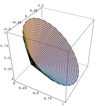
Figure 2: A spectral set of ${\bf S}_{2}$ represented in $\mathbf{R}^{3}$

It can be proved that this lifted set is not a submanifold of $S^{2}$ since it has a sharp point at the zero matrix, as suggested by its picture in $\mathbf{R}^{3}\simeq S^{2}$ (see Figure 2).     

Example 3.10 (A manifold without enough symmetry).

Let us consider the set

$$\mathcal{N}=\{(t,0,-t):t\in(-\epsilon,\epsilon)\}\,\subset\,\mathbf{R}^{3}$$

and let $\bar{x}=(0,0,0)\in\mathcal{N}$, $\sigma=(1,2,3)$. Then, $\Delta(\sigma)=\{(\alpha,\alpha,\alpha):\alpha\in\mathbf{R}\}$ and $\mathcal{N}$ is a smooth submanifold of $\mathbf{R}^{3}$ that is symmetric with respect to the affine set $\Delta(\sigma)$, but it is not locally symmetric. It can be easily proved that the set $\lambda^{-1}(\mathcal{M})$ is not a submanifold of ${\bf S}_{3}$ around the zero matrix.     

3.2 Structure of tangent and normal space

From now on

$\mathcal{M}$ is a locally symmetric $C^{2}$-submanifold of $\mathbf{R}^{n}$ of dimension $d$,

unless otherwise explicitly stated. We also denote by $T_{\mathcal{M}}(\bar{x})$ and $N_{\mathcal{M}}(\bar{x})$ its tangent and normal space at $\bar{x}\in\mathcal{M}$, respectively. In this subsection, we derive several natural properties for these two spaces, stemming from the symmetry of $\mathcal{M}$. The next lemma ensures that the tangent and normal spaces at $\bar{x}\in\mathcal{M}$ inherit the local symmetry of $\mathcal{M}$.

Lemma 3.11 (Local symmetry of $T_{\mathcal{M}}(\bar{x})$, $N_{\mathcal{M}}(\bar{x})$).

If $\bar{x}\in\mathcal{M}$ then

1. $\sigma T_{\mathcal{M}}(\bar{x})=T_{\mathcal{M}}(\bar{x})\,\,\,\text{for all }\sigma\in S^{\succsim}(\bar{x});$

2. $\sigma N_{\mathcal{M}}(\bar{x})=N_{\mathcal{M}}(\bar{x})\,\,\,\text{for all }\sigma\in S^{\succsim}(\bar{x})\,.$

Proof.  Assertion $(\ref{Tinv-i})$ follows directly from the definitions since the elements of $T_{\mathcal{M}}(\bar{x})$ can be viewed as the differentials at $\bar{x}$ of smooth paths on $\mathcal{M}$. Assertion $(\ref{Tinv-ii})$ stems from the fact that $S^{\succsim}(\sigma)$ is a group, as follows: for any $w\in T_{\mathcal{M}}(\bar{x})$, $v\in N_{\mathcal{M}}(\bar{x})$, and $\sigma\in S^{\succsim}(\sigma)$ we have $\sigma^{-1}w\in T_{\mathcal{M}}(\bar{x})$ and $\langle\sigma v,w\rangle=\langle v,\sigma^{-1}w\rangle=0$, showing that $\sigma\,v\in[T_{\mathcal{M}}(\bar{x})]^{\bot}=N_{\mathcal{M}}(\bar{x})$.     

Given a set $S\subset\mathbb{R}^{n}$, denote by $\mathrm{dist}_{S}(x):=\inf_{s\in S}\|x-s\|$ the distance of $x\in\mathbb{R}^{n}$ to $S$.

Proposition 3.12 (Local invariance of the distance).

If $\bar{x}\in\mathcal{M}$, then

$$\mathrm{dist}_{(\bar{x}+T_{\mathcal{M}}(\bar{x}))}(x)=\mathrm{dist}_{(\bar{x}+T_{\mathcal{M}}(\bar{x}))}(\sigma x)\quad\text{for any \,}\,x\in\mathbf{R}^{n}\,\text{ and }\,\sigma\in S^{\succsim}(\bar{x})\,.$$

Proof.  Assume that for some $x\in\mathbf{R}^{n}$ and $\sigma\in S^{\succsim}(\bar{x})$ we have

$$\mathrm{dist}_{(\bar{x}+T_{\mathcal{M}}(\bar{x}))}(x)<\mathrm{dist}_{(\bar{x}+T_{\mathcal{M}}(\bar{x}))}(\sigma x).$$

Then, there exists $z\in T_{\mathcal{M}}(\bar{x})$ satisfying $||x-(\bar{x}+z)||<\mathrm{dist}_{(\bar{x}+T_{\mathcal{M}}(\bar{x}))}(\sigma x)$, which yields (recalling $\sigma\bar{x}=\bar{x}$ and the fact that the norm is symmetric)

$$||x-(\bar{x}+z)||=||\sigma x-(\bar{x}+\sigma z)||<\mathrm{dist}_{(\bar{x}+T_{\mathcal{M}}(\bar{x}))}(\sigma x)$$

contradicting the fact that $\sigma z\in T_{\mathcal{M}}(\bar{x})$. The reverse inequality can be established similarly.     

Let $\bar{\pi}_{T}\colon\mathbf{R}^{n}\rightarrow\bar{x}+T_{\mathcal{M}}(\bar{x})$ be the projection onto the affine space $\bar{x}+T_{\mathcal{M}}(\bar{x})$, that is,

$$\bar{\pi}_{T}(x)=\mathrm{Proj\,}_{(\bar{x}+T_{\mathcal{M}}(\bar{x}))}(x),$$ (3.6)

and similarly, let

$$\bar{\pi}_{N}(x)=\mathrm{Proj\,}_{(\bar{x}+N_{\mathcal{M}}(\bar{x}))}(x)$$ (3.7)

denote the projection onto the affine space $\bar{x}+N_{\mathcal{M}}(\bar{x})$. We also introduce $\pi_{T}(\cdot)$ and $\pi_{N}(\cdot)$, the projections onto the tangent and normal spaces $T_{\mathcal{M}}(\bar{x})$ and $N_{\mathcal{M}}(\bar{x})$ respectively. Notice the following relationships:

$$\bar{\pi}_{T}(x)+\bar{\pi}_{N}(x)=x+\bar{x}\quad\mbox{and}\quad\bar{\pi}_{T}(x)=\pi_{T}(x)+\pi_{N}(\bar{x}).$$ (3.8)

Corollary 3.13 (Invariance of projections).

Let $\bar{x}\in\mathcal{M}$. Then, for all $x\in\mathbf{R}^{n}$ and all $\sigma\in S^{\succsim}(\bar{x})$

• $\sigma\bar{\pi}_{T}(x)=\bar{\pi}_{T}(\sigma x),$

• $\sigma\bar{\pi}_{N}(x)=\bar{\pi}_{N}(\sigma x).$

Proof.  Let $\bar{\pi}_{T}(x)=\bar{x}+u$ for some $u\in T_{\mathcal{M}}(\bar{x})$ and let $\sigma\in S^{\succsim}(\bar{x})$. Since $\sigma\bar{x}=\bar{x}$, by Proposition 3.12, and the symmetry of the norm we obtain

$$\mathrm{dist}_{(\bar{x}+T_{\mathcal{M}}(\bar{x}))}(x)=||x-(\bar{x}+u)||=||\sigma x-(\bar{x}+\sigma u)||=\mathrm{dist}_{(\bar{x}+T_{\mathcal{M}}(\bar{x}))}(\sigma x).$$

Since $\sigma u\in T_{\mathcal{M}}(\bar{x})$, we conclude $\bar{\pi}_{T}(\sigma x)=\bar{x}+\sigma u$ and assertion $(i)$ follows.

Let us now prove the second assertion. Applying (3.8) for the point $\sigma x\in\mathbf{R}^{n}$, using $(i)$ and the fact that $\sigma\bar{x}=\bar{x}$ we deduce

$$\sigma x+\bar{x} =\bar{\pi}_{T}(\sigma x)+\bar{\pi}_{N}(\sigma x)=\sigma\bar{\pi}_{T}(x)+\bar{\pi}_{N}(\sigma x)\,.$$

Applying $\sigma^{-1}$ to this equation, recalling that $\sigma^{-1}\bar{x}=\bar{x}$ and equating with (3.8) we get $(ii)$.     

The following result relates the tangent space to the stratification.

Proposition 3.14 (Tangential projection vs stratification).

Let $\bar{x}\in\mathcal{M}\cap\Delta(\sigma)$. Then, there exists $\delta>0$ such that for any $x\in\mathcal{M}\cap B(\bar{x},\delta)$ there exists $\sigma^{\prime}\in S^{\succsim}(\sigma)$ such that

$$x,\bar{\pi}_{T}(x)\in\Delta(\sigma^{\prime}).$$

Proof.  Choose $\delta>0$ so that the ball $B(\bar{x},\delta)$ intersects only those strata $\Delta(\sigma^{\prime})$ for which $\sigma^{\prime}\in S^{\succsim}(\sigma)$ (see Lemma 2.5$(ii)$). Shrinking $\delta>0$ further, if necessary, we may assume that the projection $\bar{\pi}_{T}$ is a one-to-one map between $\mathcal{M}\cap B(\bar{x},\delta)$ and its range. For any $x\in\mathcal{M}\cap B(\bar{x},\delta)$ let $u\in T_{\mathcal{M}}(\bar{x})\cap B(0,\,\delta)$ be the unique element of $T_{\mathcal{M}}(\bar{x})$ satisfying $\bar{\pi}_{T}(x)=\bar{x}+u$, or in other words such that

$$\mathrm{dist}_{\bar{x}+T_{\mathcal{M}}(\bar{x})}(x)=||x-(\bar{x}-u)||=\min_{z\in T_{\mathcal{M}}(\bar{x})}\,||(x-\bar{x})-z||\,.$$ (3.9)

Then, for some $\sigma_{1},\sigma_{2}\in S^{\succsim}(\sigma)$ we have $\bar{x}+u\in\Delta(\sigma_{1})$ and $x\in\Delta(\sigma_{2})$. In view of Lemma 3.11 and Lemma 2.5 we deduce

$$\bar{x}+\sigma_{2}u=\sigma_{2}(\bar{x}+u)\in\left(\bar{x}+T_{\mathcal{M}}(\bar{x})\right)\cap B(\bar{x},\delta).$$

We are going to show now that $\sigma_{1}\sim\sigma_{2}$. To this end, note first that

$$||x-(\bar{x}+\sigma_{2}u)||=||\sigma_{2}x-(\sigma_{2}\bar{x}+\sigma_{2}u)||=||(x-\bar{x})-u||.$$

It follows from (3.9) that $\bar{\pi}_{T}(x)=\bar{x}+\sigma_{2}u,$ thus $\sigma_{2}u=u$, which yields $\sigma_{2}(\bar{x}+u)=\bar{x}+u$, $\sigma_{1}\precsim\sigma_{2}$, by (2.5). If we assume that $\sigma_{1}\prec\sigma_{2}$ then $\sigma_{1}x\not=x$ (or else by (2.5) $P(\sigma_{1})\supseteq P(x)=P(\sigma_{2})$ and $\sigma_{1}\succsim\sigma_{2}$, a contradiction). We have $\sigma_{1}x\in\mathcal{M}\cap B(\bar{x},\delta)$, but $\sigma_{1}x\neq x$ yields $\bar{\pi}_{T}(x)\not=\bar{\pi}_{T}(\sigma_{1}x)$. Thus, there exists $v\in T_{\mathcal{M}}(\bar{x})$ with

$$\|\sigma_{1}x-(\bar{x}+v)\|<\|\sigma_{1}x-(\bar{x}+u)\|=\|x-(\bar{x}+u)\|,$$

which contradicts Proposition 3.12. Thus, $\sigma_{1}\sim\sigma_{2}$ and $x,\,\bar{x}+u\,\in\,\Delta(\sigma_{1})=\Delta(\sigma_{2})$.     

We end this subsection by the following important property that locates the tangent and normal spaces of $\mathcal{M}$ with respect to the active stratum $\Delta(\sigma)$.

Proposition 3.15 (Decomposition of $T_{\mathcal{M}}(\bar{x})$, $N_{\mathcal{M}}(\bar{x})$).

For any $\bar{x}\in\mathcal{M}\cap\Delta(\sigma)$ we have

$$\mathrm{Proj\,}_{\Delta(\sigma)^{\bot\bot}}(T_{\mathcal{M}}(\bar{x}))=T_{\mathcal{M}}(\bar{x})\cap\Delta(\sigma)^{\bot\bot}$$

which yields

$$T_{\mathcal{M}}(\bar{x})=(T_{\mathcal{M}}(\bar{x})\cap\Delta(\sigma)^{\bot\bot})\oplus(T_{\mathcal{M}}(\bar{x})\cap\Delta(\sigma)^{\bot}).$$ (3.10)

Similarly,

$$N_{\mathcal{M}}(\bar{x})=(N_{\mathcal{M}}(\bar{x})\cap\Delta(\sigma)^{\bot\bot})\oplus(N_{\mathcal{M}}(\bar{x})\cap\Delta(\sigma)^{\bot}).$$ (3.11)

Proof.  Lemma 2.7 and Lemma 3.11 show that for any $u\in T_{\mathcal{M}}(\bar{x})$ we have

$$\mathrm{Proj\,}_{\Delta(\sigma)^{\bot\bot}}(u)=\frac{1}{|S^{\succsim}(\sigma)|}\sum\limits_{\sigma^{\prime}\succsim\sigma}\sigma^{\prime}u\in T_{\mathcal{M}}(\bar{x}),$$

which yields

$$\mathrm{Proj\,}_{\Delta(\sigma)^{\bot\bot}}(T_{\mathcal{M}}(\bar{x}))\subseteq T_{\mathcal{M}}(\bar{x})\cap\Delta(\sigma)^{\bot\bot}.$$

The opposite inclusion and decomposition (3.10) are straightforward.

Let us now prove the decomposition of $N_{\mathcal{M}}(\bar{x})$. For any $u\in T_{\mathcal{M}}(\bar{x})$, by (3.10) there are (unique) vectors $u_{\bot}\in T_{\mathcal{M}}(\bar{x})\cap\Delta(\sigma)^{\bot}$ and $u_{\bot\bot}\in T_{\mathcal{M}}(\bar{x})\cap\Delta(\sigma)^{\bot\bot}$ such that $u=u_{\bot}+u_{\bot\bot}$. Since $\mathbb{R}^{n}=\Delta(\sigma)^{\bot}\oplus\Delta(\sigma)^{\bot\bot}$, we can decompose any $v\in N_{\mathcal{M}}(\bar{x})$ correspondingly as $v=v_{\bot}+v_{\bot\bot}$. Since $u_{\bot\bot},u_{\bot}\in T_{\mathcal{M}}(\bar{x})=N_{\mathcal{M}}(\bar{x})^{\bot}$ we have $\langle u_{\bot},v\rangle=0$ and $\langle u_{\bot\bot},v\rangle=0$. Using the fact that $\Delta(\sigma)^{\bot}$ and $\Delta(\sigma)^{\bot\bot}$ are orthogonal we get $\langle u_{\bot\bot},\,v_{\bot}\rangle=0$ (respectively, $\langle u_{\bot},\,v_{\bot\bot}\rangle=0$) implying that $\langle u_{\bot\bot},v_{\bot\bot}\rangle=0$ (respectively, $\langle u_{\bot},v_{\bot}\rangle=0$), and finally $\langle u,\,v_{\bot}\rangle=0$ (respectively, $\langle u,\,v_{\bot\bot}\rangle=0$). Since $u\in T_{\mathcal{M}}(\bar{x})$ has been chosen arbitrarily, we conclude $v_{\bot}\in N_{\mathcal{M}}(\bar{x})\cap\Delta(\sigma)^{\bot}$ and $v_{\bot\bot}\in N_{\mathcal{M}}(\bar{x})\cap\Delta(\sigma)^{\bot\bot}$. In other words, $N_{\mathcal{M}}(\bar{x})$ is equal to the (direct) sum of $N_{\mathcal{M}}(\bar{x})\cap\Delta(\sigma)^{\bot}$ and $N_{\mathcal{M}}(\bar{x})\cap\Delta(\sigma)^{\bot\bot}$.     

The following corollary is a simple consequence of the fact that $T_{\mathcal{M}}(\bar{x})\oplus N_{\mathcal{M}}(\bar{x})=\mathbf{R}^{n}$.

Corollary 3.16 (Decomposition of $\Delta(\sigma)^{\bot}$, $\Delta(\sigma)^{\bot\bot}$).

For any $\bar{x}\in\mathcal{M}\cap\Delta(\sigma)$ we have

$$\Delta(\sigma)^{\bot} =(\Delta(\sigma)^{\bot}\cap T_{\mathcal{M}}(\bar{x}))\oplus(\Delta(\sigma)^{\bot}\cap N_{\mathcal{M}}(\bar{x}))$$

$$\Delta(\sigma)^{\bot\bot} =(\Delta(\sigma)^{\bot\bot}\cap T_{\mathcal{M}}(\bar{x}))\oplus(\Delta(\sigma)^{\bot\bot}\cap N_{\mathcal{M}}(\bar{x})).$$

The subspaces $\Delta(\sigma)^{\bot\bot}\cap N_{\mathcal{M}}(\bar{x})$ and $T_{\mathcal{M}}(\bar{x})\cap\Delta(\sigma)^{\bot}$ in the previous statements play an important role in Section 4 when constructing adapted local equations.

3.3 Location of a locally symmetric manifold

Definition 3.5 yields important structural properties on $\mathcal{M}$. These properties are hereby quantified with the results of this section.

We need the following standard technical lemma about isometries between two Riemannian manifolds. This lemma will be used in the sequel as a link from local to global properties. Given a Riemannian manifold $M$ we recall that an open neighborhood $V$ of a point $p\in M$ is called normal if every point of $V$ can be connected to $p$ through a unique geodesic lying entirely in $V$. It is well-known (see Theorem 3.7 in [4, Chapter 3] for example) that every point of a Riemannian manifold $\mathcal{M}$ (that is, $\mathcal{M}$ is at least $C^{2}$) has a normal neighborhood. A more general version of the following lemma can be found in [7, Chapter VI], we include its proof for completeness.

Lemma 3.17 (Determination of isometries).

Let $M$, $N$ be two connected Riemannian manifolds. Let $f_{i}\colon M\rightarrow N$, $i\in\{1,2\}$ be two isometries and let $p\in M$ be such that

$$f_{1}(p)=f_{2}(p)\qquad\mbox{and}\qquad df_{1}(v)=df_{2}(v)\quad\mbox{for every }\,v\in T_{M}(p)\,.$$

Then, $f_{1}=f_{2}$.

Proof.  Every isometry mapping between two Riemannian manifolds sends a geodesic into a geodesic. For any $p\in M$ and $v\in T_{M}(p)$, we denote by $\gamma_{v,p}$ (respectively by $\tilde{\gamma}_{\bar{v},\bar{p}}$) the unique geodesic passing through $p\in M$ with velocity $v\in T_{M}(p)$ (respectively, through $\bar{p}\in N$ with velocity $\bar{v}\in T_{N}(\bar{p})$). Using uniqueness of the geodesics, it is easy to see that for all $t$

$$f_{1}(\gamma_{v,p}(t))=\tilde{\gamma}_{df_{1}(v),f_{1}(p)}(t)=\tilde{\gamma}_{df_{2}(v),f_{2}(p)}(t)=f_{2}(\gamma_{v,p}(t)).$$ (3.12)

Let $V$ be a normal neighborhood of $p$, let $q\in V$ and $[0,1]\backepsilon t\mapsto\gamma_{v,p}(t)\in M$ be the geodesic connecting $p$ to $q$ and having initial velocity $v\in T_{M}(p)$. Applying (3.12) for $t=1$ we obtain $f_{1}(q)=f_{2}(q)$. Since $q$ was arbitrarily chosen, we get $f_{1}=f_{2}$ on $V$. (Thus, since $V$ is open, we also deduce $df_{1}(v)=df_{2}(v)$ for every $v\in T_{M}(q)$.)

Let now $q$ be any point in $M$. Since connected manifolds are also path connected we can join $p$ to $q$ with a continuous path $t\in[0,1]\mapsto\delta(t)\in M$. Consider the set

$$\{t\in[0,1]:f_{1}(\delta(t))=f_{2}(\delta(t))\,\,\mbox{\rm and }\,df_{1}(v)=df_{2}(v)\,\mbox{\rm for every }v\in T_{M}(\delta(t))\}.$$ (3.13)

Since $f_{i}\colon M\rightarrow N$ and $df_{i}:TM\rightarrow TN$ ($i\in\{1,2\}$) are continuous maps, the above set is closed. further, since $f_{1}=f_{2}$ in a neighborhood of $p$ it follows that the supremum in (3.13), denoted $t_{0}$, is strictly positive. If $t_{0}\not=1$ then repeating the argument for the point $p_{1}=\delta(t_{0})$, we obtain a contradiction. Thus, $t_{0}=1$ and $f_{1}(q)=f_{2}(q)$.     

The above lemma will now be used to obtain the following result which locates the locally symmetric manifold $\mathcal{M}$ with respect to the stratification.

Corollary 3.18 (Reduction of the ambient space to $\Delta(\sigma)^{\bot\bot}$).

Let $\mathcal{M}$ be a locally symmetric manifold. If for some $\bar{x}\in\mathcal{M}$, $\sigma\in\Sigma^{n}$, and $\delta>0$ we have $\mathcal{M}\cap B(\bar{x},\delta)\subseteq\Delta(\sigma)$, then $\mathcal{M}\subseteq\Delta(\sigma)^{\bot\bot}$.

Proof.  Suppose first that $\mathcal{M}$ is strongly locally symmetric. Let $f_{1}\colon\mathcal{M}\rightarrow\mathcal{M}$ be the identity isometry on $\mathcal{M}$ and let $f_{2}\colon\mathcal{M}\rightarrow\mathcal{M}$ be the isometry determined by the permutation $\sigma,$ that is, $f_{2}(x)=\sigma x$ for all $x\in\mathcal{M}$. The assumption $\mathcal{M}\cap B(\bar{x},\delta)\subset\Delta(\sigma)$ yields that the isometries $f_{1}$ and $f_{2}$ coincide around $\bar{x}$. Thus, by Lemma 3.17 (with $M=N=\mathcal{M}$) we conclude that $f_{1}$ and $f_{2}$ coincide on $\mathcal{M}$. This shows that $\mathcal{M}\subset\Delta(\sigma)^{\bot\bot}$.

In the case when $\mathcal{M}$ is locally symmetric, assume, towards a contradiction, that there exists $\bar{\bar{x}}\in\mathcal{M}\setminus\Delta(\sigma)^{\bot\bot}$ Consider a continuous path $t\in[0,1]\mapsto p(t)\in\mathcal{M}$ with $p(0)=\bar{x}$ and $p(1)=\bar{\bar{x}}$. Find $0=t_{0}<t_{1}<\cdots<t_{s}=1$ and $\{\delta_{i}>0:i=0,\ldots,s\}$ such that $\mathcal{M}_{i}:=\mathcal{M}\cap B(p(t_{i}),\delta_{i})$ is strongly locally symmetric, the union of all $\mathcal{M}_{i}$ covers the path $p(t)$, $\mathcal{M}_{i-1}\cap\mathcal{M}_{i}\not=\emptyset$, and $\mathcal{M}_{0}\subset\Delta(\sigma)$. Let $s^{\prime}$ be the first index such that $\mathcal{M}_{s^{\prime}}\not\subset\Delta(\sigma)^{\bot\bot}$, clearly $s^{\prime}>0$. Let $x^{\prime}\in\mathcal{M}_{s^{\prime}-1}\cap\mathcal{M}_{s^{\prime}}\cap\Delta(\sigma)^{\bot\bot}$ and note that $x^{\prime}\in\Delta(\sigma^{\prime})$ for some $\sigma^{\prime}\precsim\sigma$. By the strong local symmetry of $\mathcal{M}_{s^{\prime}-1}$ and $\mathcal{M}_{s^{\prime}}$, they are both invariant under the permutation $\sigma$. Since $\sigma$ coincides with the identity on $\mathcal{M}_{s^{\prime}-1}$ and since $\mathcal{M}_{s^{\prime}-1}\cap\mathcal{M}_{s^{\prime}}$ is an open subset of $\mathcal{M}_{s^{\prime}}$, we see by Lemma 3.17 that $\sigma$ coincides with the identity on $\mathcal{M}_{s^{\prime}}$. This contradicts the fact that $\mathcal{M}_{s^{\prime}}\not\subset\Delta(\sigma)^{\bot\bot}$.     

In order to strengthen Corollary 3.18 we need to introduce a new notion.

Definition 3.19 (Much smaller permutation).

For two permutations $\sigma,\sigma^{\prime}\in\Sigma^{n}$.

• The permutation $\sigma^{\prime}$ is called much smaller than $\sigma$, denoted $\sigma^{\prime}\prec\prec\sigma$, whenever $\sigma^{\prime}\prec\sigma$ and a set in $P(\sigma^{\prime})$ is formed by merging at least two sets from $P(\sigma)$, of which at least one contains at least two elements.

• Whenever $\sigma^{\prime}\prec\sigma$ but $\sigma^{\prime}$ is not much smaller than $\sigma$ we shall write $\sigma^{\prime}\prec\sim\sigma$. In other words, if $\sigma^{\prime}\prec\sigma$ but $\sigma^{\prime}$ is not much smaller than $\sigma$, then every set in $P(\sigma^{\prime})$ that is not in $P(\sigma)$ is formed by merging one-element sets from $P(\sigma)$.

Example 3.20 (Smaller vs much smaller permutations).

The following examples illustrate the notions of Definition 3.19. We point out that part (vii) will be used frequently.

1. $(123)(45)(6)(7)\prec\prec(1)(23)(45)(6)(7)$.

2. Consider $\sigma=(167)(23)(45)$ and $\sigma^{\prime}=(1)(23)(45)(6)(7)$. In this case, $\sigma\prec\sigma^{\prime}$ but $\sigma$ is not much smaller than $\sigma^{\prime}$ because only cycles of length one are merged to form the cycles in $\sigma$. Thus, $\sigma\prec\sim\sigma^{\prime}$.

3. If $\sigma^{\prime\prime}\precsim\sigma^{\prime}$ and $\sigma^{\prime}\prec\prec\sigma$ then $\sigma^{\prime\prime}\prec\prec\sigma$.

4. It is possible to have $\sigma^{\prime}\prec\sim\sigma$ and $\sigma^{\prime\prime}\prec\sim\sigma$ but $\sigma^{\prime\prime}\prec\prec\sigma^{\prime}$, as shown by $\sigma=(1)(2)(3)(45)$, $\sigma^{\prime}=(1)(23)(45)$, and $\sigma^{\prime\prime}=(123)(45)$.

5. If $\sigma^{\prime}\prec\sigma$ and $\sigma$ fixes at most one element from $\mathbb{N}_{n}$, then $\sigma^{\prime}\prec\prec\sigma$.

6. If $\sigma\in\Sigma^{n}\setminus\mbox{\rm id}_{n}$ then $\sigma\prec\sim{\rm id}_{n}$.

7. If $\sigma^{\prime}\precsim\sigma$ and if $\sigma^{\prime}$ is not much smaller than $\sigma$, then either $\sigma^{\prime}\sim\sigma$ or $\sigma^{\prime}\prec\sim\sigma$.

8. If $\sigma^{\prime\prime}\prec\sim\sigma^{\prime}$ and $\sigma^{\prime}\prec\sim\sigma$, then $\sigma^{\prime\prime}\prec\sim\sigma$. That is, the relationship ‘not much smaller’ is transitive.     

We now describe a strengthening of Corollary 3.18. It lowers the number of strata that can intersect $\mathcal{M}$, hence better specifies the location of the manifold $\mathcal{M}$.

Corollary 3.21 (Inactive strata).

Let $\mathcal{M}$ be a locally symmetric manifold. If for some $\bar{x}\in\mathcal{M}$, $\sigma\in\Sigma^{n}$ and $\delta>0$ we have $\mathcal{M}\cap B(\bar{x},\delta)\subseteq\Delta(\sigma)$ then

$$\mathcal{M}\subseteq\Delta(\sigma)^{\bot\bot}\setminus\bigcup_{\sigma^{\prime}\prec\prec\sigma}\Delta(\sigma^{\prime}).$$

Proof.  By Corollary 3.18, we already have $\mathcal{M}\subseteq\Delta(\sigma)^{\bot\bot}$. Assume, towards a contradiction, that $\mathcal{M}\cap\Delta(\sigma^{\prime})\neq\emptyset$ for some $\sigma^{\prime}\prec\prec\sigma$. This implies in particular that $\sigma$ is not the identity permutation, see Example 3.20 (vi). Consider a continuous path connecting $\bar{x}$ with a point in $\mathcal{M}\cap\Delta(\sigma^{\prime})\neq\emptyset$. Let $z$ be the first point on that path such that $z\in\Delta(\tau)\mbox{ for some }\tau\prec\prec\sigma$. (Such a first point exists since whenever $\tau\prec\sigma$, the points in $\Delta(\tau)$ are boundary points of $\Delta(\sigma)$.) Let $\delta>0$ be such that $\mathcal{M}\cap B(z,\delta)$ is strongly locally symmetric. Let $\bar{z}\in\mathcal{M}\cap B(z,\delta)$ be a point on the path before $z$. That means $\bar{z}$ is in a stratum $\Delta(\bar{\sigma})$ with $\bar{\sigma}\prec\sim\sigma$ or $\bar{\sigma}\sim\sigma$. To summarize:

$$z\in\mathcal{M}\cap\Delta(\tau),\mbox{ where }\tau\prec\prec\sigma\mbox{ and }\bar{z}\in\mathcal{M}\cap\Delta(\bar{\sigma})\cap B(z,\delta)\not=\emptyset,\mbox{ where }\bar{\sigma}\prec\sim\sigma\mbox{ or }\bar{\sigma}\sim\sigma.$$

By Definition 3.19 and the fact $\tau\prec\prec\sigma$, we have that for some $2\leq\ell<k\leq n$, and some subset $\{a_{1},\ldots,a_{k}\}$ of $\mathbb{N}_{n},$ the cycle $(a_{1}\ldots a_{\ell})$ belongs to the cycle decomposition of $\sigma$ while the set $\{a_{1},\ldots,a_{\ell},a_{\ell+1},\ldots,a_{k}\}$ belongs to the partition $P(\tau)$. Now, since $\bar{\sigma}\prec\sim\sigma$ or $\bar{\sigma}\sim\sigma$, the cycle $(a_{1}\ldots a_{\ell})$ belongs to the cycle decomposition of $\bar{\sigma}$ as well. In order to simplify notation, without loss of generality, we assume that $a_{i}=i$ for $i\in\{1,\ldots,k\}$.

Since $\bar{z}=(\bar{z}_{1},\ldots,\bar{z}_{n})\in\mathcal{M}\cap\Delta(\bar{\sigma})\cap B(z,\delta)$ we have $\bar{z}_{1}=\cdots=\bar{z}_{\ell}=\alpha$ and $\bar{z}_{i}\neq\alpha$ for $i\in\{\ell+1,\ldots,n\}$. By the fact that $\mathcal{M}\cap B(z,\delta)$ is strongly locally symmetric, we deduce that

$$y:=\sigma_{\circ}\bar{z}\in\mathcal{M}\subset\Delta(\sigma)^{\bot\bot}\,\mbox{ for every }\sigma_{\circ}\succ\tau.$$ (3.14)

We consider separately three cases. In each one we define appropriately a permutation $\sigma_{\circ}\succ\tau$ in order to obtain a contradiction with (3.14).

Case 1.  Assume $\ell>2$ and let $\sigma_{\circ}\in\Sigma^{n}$ be constructed by exchanging the places of the elements $a_{\ell}$ and $a_{k}$ in the cycle decomposition of $\sigma$. Obviously, $\sigma_{\circ}\succ\tau$. Then, $y=\sigma_{\circ}\bar{z}=(y_{1},\ldots,y_{n})=(\bar{z}_{\sigma_{\circ}^{-1}(1)},\ldots,\bar{z}_{\sigma_{\circ}^{-1}(n)})$ and notice that we have $y_{1}=\bar{z}_{\sigma_{\circ}^{-1}(1)}=\bar{z}_{k}\neq\alpha$, while $y_{2}=\bar{z}_{\sigma_{\circ}^{-1}(2)}=\bar{z}_{1}=\alpha$. In view of (2.8) we deduce that $y\notin\Delta(\sigma)^{\bot\bot}$, a contradiction.

Case 2.  Let $\ell=2$ and suppose that $a_{3}\equiv 3$ belongs to a cycle of length one in the cycle decomposition of $\sigma$ (recall that we have assumed $a_{i}=i$, for all $i\in\{1,\dots,k\}$). In other words, $\sigma\,=\,(1\,2)(3)\sigma^{\prime}$, where $\sigma^{\prime}$ is a permutation of $\{4,\ldots,n\}$. Then, defining $\sigma_{\circ}\,:=\,(1\,3)(2)\sigma^{\prime}$ we get $y_{1}=\bar{z}_{3}\neq\alpha$ and $y_{2}=\bar{z}_{2}=\alpha$, thus again $y\notin\Delta(\sigma)^{\bot\bot}$.

Case 3.  Let $\ell=2$ and suppose that $a_{3}\equiv 3$ belongs to a cycle of length at least two in the cycle decomposition of $\sigma$. Then, $\sigma\,=\,(1\,2)\,(3\,p\,\ldots)\cdots(\ldots\,q)\,\sigma^{\prime}$, where $\sigma^{\prime}$ is a permutation of $\{k+1,\dots,n\}$, and where the union of the elements in the cycles $(1\,2)\,(3\,p\,\ldots)\cdots(\ldots\,q)$ is precisely $\{1,2,\ldots,k\}$. We define $\sigma_{\circ}\,=\,(1\,2\,3)\,(p\,\ldots)\cdots(\ldots\,q)\,\sigma^{\prime}\succ\tau$ and obtain $y_{1}=\bar{z}_{3}\neq\alpha$ and $y_{2}=\bar{z}_{1}=\alpha$, thus again $y\notin\Delta(\sigma)^{\bot\bot}$.

The proof is complete.     

3.4 The characteristic permutation $\sigma_{\ast}$ of $\mathcal{M}$

In order to better understand the structure of the lo lly symmetric manifold $\mathcal{M}$, we exhibit a permutation (more precisely, a set of equivalent permutations) that is characteristic of $\mathcal{M}$. To this end, we introduce the following sets of active permutations. (These two sets will be used only in this and the next subsections.) Define

$$\Delta(\mathcal{M}):=\{\sigma\in\Sigma^{n}:\mathcal{M}\cap\Delta(\sigma)\not=\emptyset\},$$

and

$$\Sigma_{\mathcal{M}}:=\{\sigma\in\Sigma^{n}:\exists(\bar{x}\in\mathcal{M},\delta>0)\,\,\mbox{\rm such that}\,\,\mathcal{M}\cap B(\bar{x},\delta)\subseteq\Delta(\sigma)\}\,.$$

We note that if $\sigma\in\Delta(\mathcal{M})$ then $\sigma^{\prime}\in\Delta(\mathcal{M})$ whenever $\sigma\sim\sigma^{\prime}$, and similarly for $\Sigma_{\mathcal{M}}$. The following result is straightforward.

Lemma 3.22 (Maximality of $\Sigma_{\mathcal{M}}$ in $\Delta(\mathcal{M})$).

The elements of $\Sigma_{\mathcal{M}}$ are equivalent to each other and maximal in $\Delta(\mathcal{M})$.

Proof.  It follows readily that $\Delta(\mathcal{M})\neq\emptyset$ and $\Sigma_{\mathcal{M}}\subset\Delta(\mathcal{M})$. Let $\tau\in\Delta(\mathcal{M})$ and $\sigma\in\Sigma_{\mathcal{M}}$. By Corollary 3.18 we deduce that $\mathcal{M}\subset\Delta(\sigma)^{\bot\bot}$ and by Proposition 2.3$(iii)$ that $\tau\precsim\sigma$. This proves maximality of $\sigma$ in $\Delta(\mathcal{M})$. The equivalence of the elements of $\Sigma_{\mathcal{M}}$ is obvious.     

The next lemma is, in a sense, a converse of Corollary 3.18. It shows in particular that $\Sigma_{\mathcal{M}}\neq\emptyset$.

Lemma 3.23 (Optimal reduction of the ambient space).

For a locally symmetric manifold $\mathcal{M}$, there exists a permutation $\sigma_{\ast}\in\Sigma^{n}$, such that

$$\Sigma_{\mathcal{M}}=\{\sigma\in\Sigma^{n}:\,\sigma\sim\sigma_{\ast}\}\,.$$ (3.15)

In particular, if $\mathcal{M}\subseteq\Delta(\bar{\sigma})^{\bot\bot}$ for some $\bar{\sigma}\in\Sigma^{n}$ then $\sigma_{\ast}\precsim\bar{\sigma}$.

Proof.  Assertion (3.15) follows directly from Lemma 3.22 provided one proves that $\Sigma_{\mathcal{M}}\neq\emptyset$. To do so, we assume that $\mathcal{M}\subseteq\Delta(\bar{\sigma})^{\bot\bot}$ for some $\bar{\sigma}\in\Sigma^{n}$ (this is always true for $\bar{\sigma}=\mathrm{id}_{n}$) and we prove both that $\Sigma_{\mathcal{M}}\neq\emptyset$ as well as the second part of the assertion. Notice that $\sigma\precsim\bar{\sigma}$ for all $\sigma\in\Delta(\mathcal{M})$. Let us denote by $\sigma^{\circ}:=\bigvee\Delta(\mathcal{M})$ any supremum of the nonempty set $\Delta(\mathcal{M})$ (that is, any permutation $\sigma^{\circ}$ whose partition is the supremum of the partitions $P(\sigma)$ for all $\sigma\in\Delta(\mathcal{M})$). If $\sigma^{\circ}\in\Delta(\mathcal{M}),$ then $\sigma^{\circ}\in\Sigma_{\mathcal{M}}$, $\sigma^{\circ}=\sigma_{\ast}$ and we are done. If $\sigma^{\circ}\notin\Delta(\mathcal{M})$, then choose any permutation $\sigma_{\circ}\in\Delta(\mathcal{M})$ such that

$$\{\sigma\in\Delta(\mathcal{M}):\sigma^{\circ}\succ\sigma\succ\sigma_{\circ}\}=\emptyset.$$ (3.16)

Such a permutation $\sigma_{\circ}$ exists since $\Delta(\mathcal{M})$ is a finite partially ordered set. By the definition of $\sigma_{\circ}$ there exists $\bar{x}\in\mathcal{M}\cap\Delta(\sigma_{\circ})$, and by Lemma 2.5$(\ref{key_pt2})$ we can find $\delta>0$ such that $B(\bar{x},\delta)$ intersects only strata $\Delta(\sigma)$ corresponding to permutations $\sigma\succsim\sigma_{\circ}$. If there exists $x\in\mathcal{M}\cap B(\bar{x},\delta)$ such that $x\in\Delta(\sigma)$ for some permutation $\sigma\succ\sigma_{\circ}$, then $\sigma\in\Delta(\mathcal{M})$ and by (3.16) $\sigma\sim\sigma^{\circ}$ contradicting the assumption that $\sigma^{\circ}\notin\Delta(\mathcal{M}).$ Thus, $\mathcal{M}\cap B(\bar{x},\delta)\subseteq\Delta(\sigma_{\circ})$ and $\sigma_{\circ}=\sigma_{\ast}\in\Sigma_{\mathcal{M}}$.     

Corollary 3.24 (Density of $\mathcal{M}\cap\Delta(\sigma_{*})$ in $\mathcal{M}$).

For every $\bar{x}\in\mathcal{M}$, every $\delta>0$ and $\sigma_{*}\in\Sigma_{\mathcal{M}}$, we have

$$\mathcal{M}\cap\Delta(\sigma_{*})\cap B(\bar{x},\delta)\not=\emptyset.$$

Proof.  Suppose $\bar{x}\in\mathcal{M}\cap\Delta(\sigma)$ and fix $\delta>0$ small enough so that $B(\bar{x},\delta)$ intersects only strata $\Delta(\sigma^{\prime})$ for $\sigma^{\prime}\succsim\sigma$. Then, by Lemma 2.5, we have that the manifold $\mathcal{M}^{\prime}:=\mathcal{M}\cap B(\bar{x},\delta)$ is locally symmetric. By Lemma 3.23, we obtain that $\Sigma_{\mathcal{M}^{\prime}}\not=\emptyset$. Since $\Sigma_{\mathcal{M}^{\prime}}\subset\Sigma_{\mathcal{M}}$, and all permutations in $\Sigma_{\mathcal{M}}$ are equivalent, we have $\Sigma_{\mathcal{M}^{\prime}}=\Sigma_{\mathcal{M}}$. Thus, $\mathcal{M}^{\prime}\cap B(\bar{y},\rho)\subset\Delta(\sigma_{*})$ for $\bar{y}\in\mathcal{M}^{\prime}\subset\mathcal{M}$ and some $\rho>0$, whence the result follows.     

Clearly, if ${\rm id}_{n}\in\Sigma_{\mathcal{M}}$, then $\Sigma_{\mathcal{M}}=\{{\rm id}_{n}\}$. In particular, we have the following easy result.

Corollary 3.25.

For a locally symmetric manifold $\mathcal{M}\subset\mathbf{R}^{n}$, we have

$$\sigma_{*}={\rm id}_{n}\,\,\,\Longleftrightarrow\,\,\,\mathcal{M}\cap\Delta({\rm id}_{n})\not=\emptyset.$$

Proof.  The necessity is obvious, while the sufficiency follows from Lemma 3.22, since ${\rm id}_{n}\in\Delta(\mathcal{M})$ is the unique maximal element of $\Sigma^{n}$.     

Thus, the permutation $\sigma_{\ast}$ is naturally associated with the locally symmetric manifold $\mathcal{M}$ via the property

$$\exists(\bar{x}\in\mathcal{M},\delta>0)\,\,\mbox{\rm such that}\,\,\mathcal{M}\cap B(\bar{x},\delta)\subseteq\Delta(\sigma_{\ast}).$$ (3.17)

Notice that $\sigma_{\ast}$ is unique modulo $\sim$, and will be called characteristic permutation of $\mathcal{M}$. Even though the definition of the characteristic permutation $\sigma_{\ast}$ is local, it has global properties stemming from Corollary 3.21, that is,

$$\mathcal{M}\ \subseteq\ \Delta(\sigma_{\ast})^{\bot\bot}\setminus\!\bigcup_{\sigma\prec\prec\sigma_{\ast}}\Delta(\sigma)\ =\bigcup_{{\scriptsize\begin{array}[]{c}\sigma\sim\sigma_{\ast}\\[-1.50694pt] \sigma\prec\sim\sigma_{\ast}\end{array}}}\Delta(\sigma)\ \subseteq\ \Delta(\sigma_{\ast})^{\bot\bot}\,,$$ (3.18)

and $\sigma_{*}$ is the minimal permutation for which (3.18) holds. The above formula determines precisely which strata can intersect $\mathcal{M}$. Indeed, if $\sigma\in\Delta(\mathcal{M})$ then necessarily either $\sigma\sim\sigma_{\ast}$ or $\sigma\prec\sim\sigma_{\ast}$. Notice also that when $\sigma\prec\sim\sigma_{\ast}$, every set in $P(\sigma)$, which is not in $P(\sigma_{\ast})$, is obtained by merging sets of length one from $P(\sigma_{\ast})$. Another consequence is the following relation:

$$T_{\mathcal{M}}(\bar{x})\subset\Delta(\sigma_{\ast})^{\bot\bot}\qquad\text{for all }\bar{x}\in\mathcal{M}\,.$$ (3.19)

Remark 3.26.

Observe that for any fixed permutation $\sigma_{*}\in\Sigma^{n}$, the set

$$\bigcup_{{\scriptsize\begin{array}[]{c}\sigma\sim\sigma_{\ast}\\[-1.50694pt] \sigma\prec\sim\sigma_{\ast}\end{array}}}\Delta(\sigma)$$

is a locally symmetric manifold with characteristic permutation $\sigma_{*}$. On the other hand, (3.18) shows that the affine space $\Delta(\sigma)^{\bot\bot}$ is a locally symmetric manifold if (and only if) $\sigma\in\Sigma^{n}$ is equal to $\mbox{id}_{n}$ or is a cycle of length $n$.     

We conclude with another fact about the characteristic permutation, that stems from the assumption $\mathcal{M}\cap\mathbf{R}^{n}_{\geq}\not=\emptyset$ (see Definition 3.5). Though (3.18) describes well the strata that can intersect the manifold $\mathcal{M}$ (which is going to be sufficient for most of our needs) we still need to say more about a slightly finer issue - a necessary condition for a stratum to intersect $\mathcal{M}\cap\mathbf{R}^{n}_{\geq}$.

Lemma 3.27.

Suppose that $\bar{x}\in\mathcal{M}\cap\mathbf{R}^{n}_{\geq}\cap\Delta(\sigma)$. Then, every set $I_{i}$ of the partition

$$P(\sigma)=\{I_{1},\ldots,I_{\kappa+m}\}$$

contains consecutive integers from $\mathbb{N}_{n}$.

Proof.  The lemma is trivially true, for sets $I_{i}$ with cardinality one. So, suppose on the contrary, that for some $\ell\in\{1,\ldots,\kappa+m\}$, the set $I_{\ell}$ contains at least two elements but does not contain consecutive numbers from $\mathbb{N}_{n}$. That is, there are three indexes $i,j,k\in\mathbb{N}_{n}$ with $i<j<k$ such that $i,k\in I_{\ell}$ but $j\not\in I_{\ell}$. Then, the fact $\bar{x}\in\Delta(\sigma)$ implies that $\bar{x}_{i}=\bar{x}_{k}$, while the fact that $\bar{x}\in\mathbf{R}^{n}_{\geq}$ implies that $\bar{x}_{i}\geq\bar{x}_{j}\geq\bar{x}_{k}$. We obtain $\bar{x}_{i}=\bar{x}_{j}=\bar{x}_{k}$, which contradicts the assumption $j\not\in I_{\ell}$.     

Lemma 3.27 has consequences for the characteristic permutation $\sigma_{*}$ of $\mathcal{M}$.

Theorem 3.28 (Characteristic partition $P(\sigma_{*})$).

Every set in the partition $P(\sigma_{*})$ contains consecutive integers from $\mathbb{N}_{n}$.

Proof.  Let $\sigma_{\ast}\in\Sigma_{\mathcal{M}}$ be the characteristic permutation of $\mathcal{M}$. Since $\mathcal{M}\cap\mathbf{R}^{n}_{\geq}\not=\emptyset$ by Definition 3.5, there is a stratum $\Delta(\sigma)$ intersecting $\mathcal{M}\cap\mathbf{R}^{n}_{\geq}$. Formula (3.18) implies that $\sigma$ is not much smaller than $\sigma_{*}$, i.e. we have $\sigma\sim\sigma_{\ast}$ or $\sigma\prec\sim\sigma_{\ast}$. If a set $I^{*}_{i}\in P(\sigma_{*})$ has more than one element, then it must be an element of the partition $P(\sigma)$ as well, by the fact that $\sigma$ is not much smaller than $\sigma_{*}$. Thus, $I^{*}_{i}$ contains consecutive elements from $\mathbb{N}_{n}$, by Lemma 3.27.     

For example, according to Theorem 3.28, the permutation $(1)(274)(35)(6)\in\Sigma^{7}$ cannot be the characteristic permutation of any locally symmetric manifold $\mathcal{M}$ in $\mathbf{R}^{7}$ (that intersects $\mathbf{R}^{7}_{\geq}$).

Let us illustrate the limitations imposed by the previous result. Suppose that $n=12$ and the partition $P(\sigma_{*})$ of $\mathbb{N}_{12}$ corresponding to $\sigma_{*}\in\Sigma^{12}$ is

$$P(\sigma_{*})=\{\{1\},\{2\},\{3,4,5\},\{6\},\{7\},\{8\},\{9\},\{10,11,12\}\}.$$

Pick a permutation $\sigma\in\Sigma^{12}$ with partition

$$P(\sigma)=\{\{1\},\{2\},\{3,4,5\},\{6,8,9\},\{7\},\{10,11,12\}\}.$$

In comparison with Formula (3.18), $\sigma$ is not much smaller than $\sigma_{*}$ but the stratum $\Delta(\sigma)$ does not intersect $\mathcal{M}\cap\mathbf{R}^{n}_{\geq}$. Thus, the set of strata that may intersect with $\mathcal{M}\cap\mathbf{R}^{n}_{\geq}$ is further reduced.

3.5 Canonical decomposition induced by $\sigma_{\ast}$

We explain in this subsection that the characteristic permutation $\sigma_{\ast}$ of $\mathcal{M}$ induces a decomposition of the space $\mathbf{R}^{n}$ that will be used later to control the lift into the matrix space ${\bf S}^{n}$. We consider the partition $P(\sigma_{*})$ of $\mathbb{N}_{n}$ associated with $\sigma_{*}$, and we define

$$m_{\ast}:=\mbox{ number of sets in $P(\sigma_{\ast})$ that have more than one element},$$ (3.20)

and

$${\kappa_{\ast}}:=\mbox{ number of sets in $P(\sigma_{\ast})$ with exactly one element.}$$ (3.21)

In other words, ${\kappa_{\ast}}$ is the number of elements of $\mathbb{N}_{n}$ that are fixed by the permutation $\sigma_{\ast}$, or equivalently, ${\kappa_{\ast}}:=|\mathbb{N}_{n}\setminus\mathrm{supp}(\sigma_{\ast})|$. Hence, we have

$$P(\sigma_{\ast}):=\{I_{1}^{\ast},\ldots,I_{\kappa_{\ast}}^{\ast},I_{{\kappa_{\ast}}+1}^{\ast},\ldots,I_{{\kappa_{\ast}}+m_{\ast}}^{\ast}\},$$ (3.22)

where $\{I_{1}^{\ast},\ldots,I_{\kappa_{\ast}}^{\ast}\}$ are the blocks of size one. The following example treats the particular case where $\sigma_{\ast}$ has at most one cycle of length one.

Example 3.29 (Case: ${\kappa_{\ast}}=0$ or $1$).

The assumption ${\kappa_{\ast}}\in\{0,1\}$ means that the permutation $\sigma_{\ast}$ fixes at most one element, or in other words, for every $x\in\mathcal{M}$ at most one coordinate of the vector $x=(x_{1},\dots,x_{n})$ is not repeated. In this case, by Example 3.20(v), every $\sigma$ that is smaller than $\sigma_{*}$ is much smaller than $\sigma_{*}$ and therefore (3.18) together with Proposition 2.3$(iii)$ yields $\mathcal{M}\subset\Delta(\sigma_{\ast})$.     

The partition of the characteristic permutation $\sigma_{\ast}$ of $\mathcal{M}$ yields a canonical split of $\mathbf{R}^{n}$ associated to $\mathcal{M}$, as a direct sum of two parts, the spaces $\mathbf{R}^{\kappa_{\ast}}$ and $\mathbf{R}^{n-{\kappa_{\ast}}}$, as follows: any vector $x\in\mathbf{R}^{n}$ is represented as

$$x=x^{F}\otimes x^{M}$$ (3.23)

where

• $x^{F}\in\mathbf{R}^{{\kappa_{\ast}}}$ is the subvector of $x\in\mathbf{R}^{n}$ obtained by collecting from $x$ the coordinates that have indices in $\mathbb{N}_{n}\setminus\mathrm{supp}(\sigma_{\ast})$ and preserving their relative order;

• $x^{M}\in\mathbf{R}^{n-{\kappa_{\ast}}}$ is the subvector of $x\in\mathbf{R}^{n}$ obtained by collecting from $x$ the remaining $n-{\kappa_{\ast}}$ coordinates, preserving their order again.

It is readily seen that the canonical split is linear and also a reversible operation. Reversibility means that given any two vectors $x^{F}\in\mathbf{R}^{\kappa_{*}}$ and $x^{M}\in\mathbf{R}^{n-\kappa_{*}}$, there is a unique vector $x^{F}\otimes x^{M}\in\mathbf{R}^{n}$, such that

$$(x^{F}\otimes x^{M})^{F}=x^{F}\quad\mbox{ and }\quad(x^{F}\otimes x^{M})^{M}=x^{M}.$$

This operation is called canonical product.

Example 3.30.

If $\sigma_{*}=(1)(23)(4)(567)(8)\in\Sigma^{8}$ and $x\in\mathbf{R}^{8}$ then, $x^{F}=(x_{1},x_{4},x_{8})$ and $x^{M}=(x_{2},x_{3},x_{5},x_{6},x_{7})$. Conversely, if

$$x^{F}=(a_{1},a_{2},a_{3})\qquad\mbox{and}\qquad x^{M}=(b_{1},b_{2},b_{3},b_{4},b_{5})$$

then

$$x^{F}\otimes x^{M}=(a_{1},b_{1},b_{2},a_{2},b_{3},b_{4},b_{5},a_{3}).$$

In addition, if $x\in\mathbf{R}^{8}_{\geq}$ then $x^{F}\in\mathbf{R}^{3}_{\geq}$ and $x^{M}\in\mathbf{R}^{5}_{\geq}$, but the converse is not true: if $x^{F}\in\mathbf{R}^{3}_{\geq}$ and $x^{M}\in\mathbf{R}^{5}_{\geq}$ then in general, $x^{F}\otimes x^{M}$ is not in $\mathbf{R}^{8}_{\geq}$.    

Furthermore, if $\sigma\in\Sigma^{n}$ is any permutation whose cycles do not contain elements simultaneously from $\mathrm{supp}(\sigma_{*})$ and $\mathbb{N}_{n}\setminus\mathrm{supp}(\sigma_{*})$, then it can be decomposed as

$$\sigma=\sigma^{F}\circ\sigma^{M},$$ (3.24)

where

• $\sigma^{F}\in\Sigma^{\kappa_{\ast}}$ is obtained by those cycles of $\sigma$ that contain only elements from $\mathbb{N}_{n}\setminus\mathrm{supp}(\sigma_{\ast})$,

• $\sigma^{M}\in\Sigma^{n-{\kappa_{\ast}}}$ is obtained from the remaining cycles of $\sigma$ (those that do not contain any element of $\mathbb{N}_{n}\setminus\mathrm{supp}(\sigma_{\ast})$).

Observe that $\sigma$ is the infimum of $\sigma^{F}$ and $\sigma^{M}$ ($\sigma=\sigma^{F}\wedge\sigma^{M}$). We refer to (3.24) as the $(F,M)$-decomposition of the permutation $\sigma$. For example, applying this decomposition to $\sigma_{\ast}$ yields

$$\sigma_{\ast}^{F}=\mathrm{id}_{{\kappa_{\ast}}},$$ (3.25)

where $\mathrm{id}_{{\kappa_{\ast}}}$ is the identity permutation on the set $\mathbb{N}_{n}\setminus\mathrm{supp}(\sigma_{\ast})$. Note that in the particular case ${\kappa_{\ast}}=n$, we have $\sigma_{\ast}=\operatorname*{id}_{n}$, all coefficients of $x\in\Delta(\sigma_{\ast})$ are different, and $x=x^{F}$.

The following proposition is a straightforward consequence of (3.25) and Example 3.20(v).

Proposition 3.31 ($(F,M)$-decomposition for $\sigma\prec\sim\sigma_{\ast}$).

The following equivalences hold:

$$\sigma\sim\sigma_{\ast}\ \iff\ \sigma^{F}=\mathrm{id}_{\kappa_{\ast}}\quad\text{and}\quad\sigma^{M}\sim{\sigma_{\ast}}^{M}$$

and

$$\sigma\prec\sim\sigma_{\ast}\ \iff\ \sigma^{F}\prec\mathrm{id}_{\kappa_{\ast}}\quad\text{and}\quad\sigma^{M}\sim{\sigma_{\ast}}^{M}.$$

Note that the $(F,M)$-decomposition is not going to be applied to permutations $\sigma\in\Sigma^{n}$ that are much smaller than $\sigma_{\ast}$, since these permutations may have a cycle containing elements from both $\mathrm{supp}(\sigma_{\ast})$ and $\mathbb{N}_{n}\setminus\mathrm{supp}(\sigma_{\ast})$. In fact, (3.24) can be applied only to permutations $\tau\in S^{\succsim}(\sigma)$ with $\sigma\in\Delta(\mathcal{M})$, as explained in the following result, whose proof is straightforward.

Proposition 3.32 ($(F,M)$-decomposition for active permutations).

Let $\sigma\in\Delta(\mathcal{M})$ and $\tau\in S^{\succsim}(\sigma)$. Then, $\tau$ admits $(F,M)$-decomposition $\tau=\tau^{F}\circ\tau^{M}$ given in (3.24) with

$$\sigma^{F}\precsim\tau^{F}\precsim\mathrm{id}_{{\kappa_{\ast}}}\qquad\text{and}\qquad\sigma_{\ast}^{M}\sim\sigma^{M}\precsim\tau^{M}.$$

3.6 Reduction of the normal space

In this section we fix a point $\bar{x}$ and a permutation $\sigma$ such that $\bar{x}\in\mathcal{M}\cap\Delta(\sigma)$, and reduce the relevant (active) part of the tangent and normal space with respect to the canonical split

$$\mathbf{R}^{n}=\mathbf{R}^{{\kappa_{\ast}}}\otimes\mathbf{R}^{n-{\kappa_{\ast}}}$$ (3.26)

induced by the characteristic permutation $\sigma_{\ast}$ of $\mathcal{M}$.

Let us consider any permutation $\tau\in\Sigma^{n}$ for which the decomposition (3.24)

$$\tau=\tau^{F}\circ\tau^{M}$$

makes sense (that is, $\tau\in S^{\succsim}(\sigma)$, where $\sigma\sim\sigma_{\ast}$ or $\sigma\prec\sim\sigma_{\ast}$). Then, we can either consider $\tau^{F}$ as an element of $\Sigma^{n}$ (giving rise to a stratum $\Delta(\tau^{F})\subset\mathbf{R}^{n}$) or as an element of $\Sigma^{\kappa_{\ast}}$ (acting on the space $\mathbb{R}^{\kappa_{\ast}}$). In this latter case, and in other to avoid ambiguities, we introduce the notation

$$[\Delta(\tau^{F})_{\mathbb{R}^{\kappa_{\ast}}}]:=\{z\in\mathbb{R}^{\kappa_{\ast}}:P(z)=P(\tau^{F})\}$$ (3.27)

to refer to the corresponding stratum of $\mathbb{R}^{\kappa_{\ast}}$. The notations $[\Delta(\tau^{F})_{\mathbb{R}^{\kappa_{\ast}}}]^{\bot}$, $[\Delta(\tau^{F})_{\mathbb{R}^{\kappa_{\ast}}}]^{\bot\bot}$ refer thus to the corresponding linear subspaces of $\mathbb{R}^{\kappa_{\ast}}$. We do the same for the stratum $[\Delta(\tau^{M})_{\mathbb{R}^{n-\kappa_{\ast}}}]$ (and the linear subspaces $[\Delta(\tau^{M})_{\mathbb{R}^{n-\kappa_{\ast}}}]^{\bot}$, $[\Delta(\tau^{M})_{\mathbb{R}^{n-\kappa_{\ast}}}]^{\bot\bot}$), whenever the permutation $\tau^{M}$ is considered as an element of $\Sigma^{n-\kappa_{\ast}}$ acting on $\mathbb{R}^{n-\kappa_{\ast}}$. A careful glance at the formulas (2.7) and (2.8) reveals the following relations:

$$\Delta(\tau^{F})^{\bot}=[\Delta(\tau^{F})_{\mathbb{R}^{\kappa_{\ast}}}]^{\bot}\otimes\{0\}_{n-\kappa_{\ast}}\qquad\text{and}\qquad\Delta(\tau^{M})^{\bot}=\{0\}_{\kappa_{\ast}}\otimes[\Delta(\tau^{M})_{\mathbb{R}^{n-\kappa_{\ast}}}]^{\bot}\text{ ;}$$ (3.28)

and respectively,

$$\Delta(\tau^{F})^{\bot\bot}=[\Delta(\tau^{F})_{\mathbb{R}^{\kappa_{\ast}}}]^{\bot\bot}\otimes\mathbb{R}^{n-\kappa_{\ast}}\qquad\text{ and}\qquad\Delta(\tau^{M})^{\bot\bot}=\mathbb{R}^{\kappa_{\ast}}\otimes[\Delta(\tau^{M})_{\mathbb{R}^{n-\kappa_{\ast}}}]^{\bot\bot}\text{ .}$$ (3.29)

It follows easily from (2.12) and (3.29) that

$$\Delta(\tau)^{\bot\bot}=[\Delta(\tau^{F})_{\mathbb{R}^{\kappa_{\ast}}}]^{\bot\bot}\otimes[\Delta(\tau^{M})_{\mathbb{R}^{n-\kappa_{\ast}}}]^{\bot\bot}.$$ (3.30)

It also follows easily that

$$\Delta(\tau)^{\bot}=[\Delta(\tau^{F})_{\mathbb{R}^{\kappa_{\ast}}}]^{\bot}\otimes[\Delta(\tau^{M})_{\mathbb{R}^{n-\kappa_{\ast}}}]^{\bot}.$$ (3.31)

In the sequel, we apply the canonical split (3.26) to the tangent space $T_{\mathcal{M}}(\bar{x})$. In view of (3.19) and (3.30) for $\tau=\sigma_{\ast}$ and the fact that $\sigma_{\ast}^{M}\sim\sigma^{M}$ (see Proposition 3.31), we obtain that for every $w\in T_{\mathcal{M}}(\bar{x})$

$$w=w^{F}\otimes w^{M}\quad\text{ where }\quad w^{F}\in\mathbb{R}^{{\kappa_{\ast}}}\quad\text{and}\quad w^{M}\in[\Delta(\sigma^{M})_{\mathbb{R}^{n-\kappa_{\ast}}}]^{\bot\bot}\,\subset\mathbb{R}^{n-\kappa_{\ast}},$$ (3.32)

where each coordinate of $w^{M}$ is repeated at least twice.

The following theorem reveals a analogous relationship for the canonical split of the normal space $N_{\mathcal{M}}(\bar{x})$ of $\mathcal{M}$ at $\bar{x}$. It is the culmination of most of the developments up to now and thus the most important auxiliary result in this work. We start by a technical result.

Lemma 3.33.

Let $\bar{x}\in\mathcal{M}\cap\Delta(\sigma)$ and let the $(F,M)$-decomposition of $\sigma$ be $\sigma=\sigma^{F}\circ\sigma^{M}$. Let the partition of $\mathbb{N}_{\kappa_{*}}$ defined by $\sigma^{F}$ be $P(\sigma^{F})=\{I_{1},\ldots,I_{m}\}$. Then, for every $\epsilon>0$, there exists $w\in T_{\mathcal{M}}(\bar{x})\cap B(0,\epsilon)$, such that in vector $w^{F}\in\mathbb{R}^{\kappa_{\ast}}$ every subvector $w^{F}_{I_{i}}$ has distinct coordinates, for $i\in\mathbb{N}_{m}$.

Proof.  By Corollary 3.24, we can chose $x\in\mathcal{M}\cap\Delta(\sigma_{\ast})$ arbitrarily close to $\bar{x}$. Now apply Proposition 3.14 to $\bar{x}$ and $x$ to conclude that $x,\bar{\pi}_{T}(x)\in\Delta(\sigma^{\prime})$ for some $\sigma^{\prime}\succsim\sigma$. Necessarily, we have $\sigma^{\prime}\sim\sigma_{*}$, implying that $x,\bar{\pi}_{T}(x)\in\Delta(\sigma_{*})$. This shows that $(\bar{\pi}_{T}(x))^{F}$ has distinct coordinates. In other words, there is a vector $w\in T_{\mathcal{M}}(\bar{x})$ such that $(\bar{\pi}_{T}(x))^{F}=(\bar{x}+w)^{F}=\bar{x}^{F}+w^{F}$ has distinct coordinates. Since $x$ can be chosen arbitrarily close to $\bar{x}$, we can assume that $w$ is arbitrarily close to $0$. Finally, since $\bar{x}^{F}\in[\Delta(\sigma^{F})_{\mathbf{R}^{\kappa_{*}}}]$ and $w^{F}=(\bar{x}^{F}+w^{F})-\bar{x}^{F}$ we conclude that $w^{F}_{I_{i}}$ has distinct coordinates, for $i\in\mathbb{N}_{m}$.     

Theorem 3.34 (Reduction of the normal space).

Let $\bar{x}\in\mathcal{M}\cap\Delta(\sigma)$ and $v\in N_{\mathcal{M}}(\bar{x})$. Let $v=v^{F}\otimes v^{M}$ and $\sigma=\sigma^{F}\circ\sigma^{M}$ be the canonical split and the $(F,M)$-decomposition defined in (3.23) and (3.24) respectively. Then,

$$v^{F}\in[\Delta(\sigma^{F})_{\mathbb{R}^{\kappa_{\ast}}}]^{\bot\bot}\text{.}$$ (3.33)

Proof.  Let us decompose $v\in N_{\mathcal{M}}(\bar{x})$ according to Proposition 3.15, that is, $v=v_{\bot\bot}+v_{\bot}$ where

$$v_{\bot\bot}\in N_{\mathcal{M}}(\bar{x})\cap\Delta(\sigma)^{\bot\bot}\text{\quad and}\quad v_{\bot}\in N_{\mathcal{M}}(\bar{x})\cap\Delta(\sigma)^{\bot}.$$

Then,

$$v^{F}=v_{\bot\bot}^{F}+v_{\bot}^{F}\text{\quad and}\quad v^{M}=v_{\bot\bot}^{M}+v_{\bot}^{M}.$$

Since $v_{\bot}\in\Delta(\sigma)^{\bot}$ it follows by (3.31) that $v_{\bot}^{F}\in[\Delta(\sigma^{F})_{\mathbb{R}^{\kappa_{\ast}}}]^{\bot}$. Note further that since $\sigma\in\Delta(\mathcal{M})$, we have $\sigma\prec\sim\sigma_{\ast}$, see (3.18). Let now $w=w^{F}\otimes w^{M}$ be any element of $T_{\mathcal{M}}(\bar{x})$ for which $w^{F}\in\mathbb{R}^{\kappa_{\ast}}$ has the property described in Lemma 3.33. Pick any permutation $\tau\in S^{\succsim}(\sigma)$. Then, $\tau$ admits a canonical decomposition $\tau=\tau^{F}\circ\tau^{M}$ with $\tau^{M}\succsim\sigma^{M}$ and $\tau^{F}\succsim\sigma^{F}$ (Proposition 3.32). It follows that $(\tau w)^{F}=\tau^{F}w^{F}$, $(\tau w)^{M}=\tau^{M}w^{M}=w^{M}$ (in view of (3.32)) and $\tau w\in T_{\mathcal{M}}(\bar{x})$ (in view of Lemma 3.11$(\ref{Tinv-i})$). Thus, we deduce successively:

$$0=\langle v_{\perp},\tau w\rangle=\langle v_{\perp}^{F},(\tau w)^{F}\rangle\,+\,\langle v_{\perp}^{M},(\tau w)^{M}\rangle=\langle v_{\perp}^{F},\tau^{F}w^{F}\rangle\,+\,\langle v_{\perp}^{M},w^{M}\rangle.$$

This yields

$$\langle v_{\perp}^{F},\tau^{F}w^{F}\rangle\,=-\langle v_{\perp}^{M},w^{M}\rangle,$$

which in view of Corollary 5.2 in the Appendix (applied to $x:=v_{\perp}^{F}\in[\Delta(\sigma^{F})_{\mathbb{R}^{\kappa_{\ast}}}]^{\bot}$, $\sigma:=\sigma^{F}$, $y:=w^{F}$, $\sigma^{\prime}:=\tau^{F}$, and $\alpha:=-\langle v_{\perp}^{M},w^{M}\rangle$) yields $v_{\perp}^{F}=\{0\}_{\kappa_{\ast}}$. Finally, let us recall that $v_{\bot\bot}\in\Delta(\sigma)^{\bot\bot},$ which in view of (3.30) yields $v_{\bot\bot}^{F}\in[\Delta(\sigma^{F})_{\mathbb{R}^{\kappa_{\ast}}}]^{\bot\bot}$. Thus, $v^{F}=v_{\bot\bot}^{F}\in[\Delta(\sigma^{F})_{\mathbb{R}^{\kappa_{\ast}}}]^{\bot\bot}$. The proof is complete.     

3.7 Tangential parametrization of a locally symmetric manifold

In this subsection we consider a local equation of the manifold, called tangential parametrization. We briefly recall some general properties of this parametrization (for any manifold $\mathcal{M}$) and then, we make use of Theorem 3.34 to specify it to our context.

The local inversion theorem asserts that for some $\delta>0$ sufficiently small the restriction of $\bar{\pi}_{T}$ around $\bar{x}\in\mathcal{M}$

$$\bar{\pi}_{T}\colon\mathcal{M}\cap B(\bar{x},\delta)\rightarrow\bar{x}+T_{\mathcal{M}}(\bar{x})$$

is a diffeomorphism of $\mathcal{M}\cap B(\bar{x},\delta)$ onto its image (which is an open neighborhood of $\bar{x}$ relatively to the affine space $\bar{x}+T_{\mathcal{M}}(\bar{x})$). Then, there exists a smooth map

$$\phi\colon(\bar{x}+T_{\mathcal{M}}(\bar{x}))\cap B(\bar{x},\delta)\rightarrow N_{\mathcal{M}}(\bar{x}),$$ (3.34)

such that

$$\mathcal{M}\cap B(\bar{x},\delta)=\{y\in\mathbf{R}^{n}:y=x+\phi(x),\,x\in(\bar{x}+T_{\mathcal{M}}(\bar{x}))\cap B(\bar{x},\delta)\}.$$ (3.35)

In words, the function $\phi$ measures the difference between the manifold and its tangent space. Obviously, $\phi\equiv 0$ if $\mathcal{M}$ is an affine manifold around $\bar{x}$. Note that, technically, the domain of the map $\phi$ is the open set $\bar{\pi}_{T}(\mathcal{M}\cap B(\bar{x},\delta))$, which may be a proper subset of $(\bar{x}+T_{\mathcal{M}}(\bar{x}))\cap B(\bar{x},\delta)$. Even though we keep this in mind, it will not have any bearing on the developments in the sequel. Thus, for sake of readability we will avoid introducing more precise but also more complicated notation, for example, rectangular neighborhoods around $\bar{x}$.

We say that the map $\psi\colon(\bar{x}+T_{\mathcal{M}}(\bar{x}))\cap B(\bar{x},\delta)\rightarrow\mathcal{M}\cap B(\bar{x},\delta)$ defined by

$$\psi(x)=x+\phi(x)$$ (3.36)

is the tangential parametrization of $\mathcal{M}$ around $\bar{x}$. This function is indeed smooth, one-to-one and onto, with a full rank Jacobian matrix $J\psi(\bar{x})$: it is a local diffeomorphism at $\bar{x}$, and more precisely its inverse is $\bar{\pi}_{T}$, that is, locally $\bar{\pi}_{T}(\psi(x))=x$. The above properties of $\psi$ hold for any manifold.

Let us return to the situation where $\mathcal{M}$ is a locally symmetric manifold. We consider its characteristic permutation $\sigma_{\ast}$, and we make the following assumption on the neighborhood.

Assumption 3.35.

Let $\mathcal{M}$ be a locally symmetric $C^{2}$-submanifold of $\mathbf{R}^{n}$ of dimension $d$ and of characteristic permutation $\sigma_{*}$. We consider $\bar{x}\in\mathcal{M}\cap\Delta(\sigma)$ and we take $\delta>0$ small enough so that:

1. $B(\bar{x},\delta)$ intersects only strata $\Delta(\sigma^{\prime})$ with $\sigma^{\prime}\succsim\sigma$ (recall Lemma 2.5);

2. $\mathcal{M}\cap B(\bar{x},\delta)$ is a strongly locally symmetric manifold;

3. $\mathcal{M}\cap B(\bar{x},\delta)$ is diffeomorphic to its projection on $\bar{x}+T_{\mathcal{M}}(\bar{x})$; in other words, the tangential parametrization holds.

This ensures that

$$\Delta(\sigma)^{\bot\bot}\cap B(\bar{x},\delta)=\Delta(\sigma)\cap B(\bar{x},\delta).$$

This situation enables us to specify the general properties of the tangential parametrization.

Lemma 3.36 (Tangential parametrization).

Let $\bar{x}\in\mathcal{M}\cap\Delta(\sigma)$. Then, the function $\phi$ in the tangential parametrization satisfies

$$\phi(x)\in N_{\mathcal{M}}(\bar{x})\cap\Delta(\sigma)^{\bot\bot}.$$ (3.37)

Moreover, for all $x\in(\bar{x}+T_{\mathcal{M}}(\bar{x}))\cap B(\bar{x},\delta)$ and for all $\sigma^{\prime}\in S^{\succsim}(\sigma)$ we have

$$\psi(\sigma^{\prime}x)=\sigma^{\prime}\psi(x)$$ (3.38)

and

$$\phi(\sigma^{\prime}x)=\sigma^{\prime}\phi(x)=\phi(x).$$ (3.39)

Proof.  Recalling the direct decomposition of the normal space (see Proposition 3.15) we define the mappings $\phi_{\bot\bot}(x)$ and $\phi_{\bot}(x)$ as the projections of $\phi(x)$ onto $N_{\mathcal{M}}(\bar{x})\cap\Delta(\sigma)^{\bot\bot}$ and $N_{\mathcal{M}}(\bar{x})\cap\Delta(\sigma)^{\bot}$ respectively. Thus, (3.36) becomes

$$\psi(x)=x+\phi_{\bot\bot}(x)+\phi_{\bot}(x).$$ (3.40)

Splitting each term in both sides of Equation (3.40) in view of the canonical split defined in (3.23), we obtain

$$\left(\begin{array}[]{c}\psi^{F}(x)\vskip 3.0pt plus 1.0pt minus 1.0pt\\ \psi^{M}(x)\end{array}\right)=\left(\begin{array}[]{c}x^{F}\vskip 3.0pt plus 1.0pt minus 1.0pt\\ x^{M}\end{array}\right)+\left(\begin{array}[]{c}\phi_{\bot\bot}^{F}(x)\vskip 3.0pt plus 1.0pt minus 1.0pt\\ \phi_{\bot\bot}^{M}(x)\end{array}\right)+\left(\begin{array}[]{c}\phi_{\bot}^{F}(x)\vskip 3.0pt plus 1.0pt minus 1.0pt\\ \phi_{\bot}^{M}(x)\end{array}\right).$$

We look at the second line of this vector equation. Since

$$\phi_{\bot\bot}(x)\in N_{\mathcal{M}}(\bar{x})\cap\Delta(\sigma)^{\bot\bot}\,\mbox{ and }\,\phi_{\bot}(x)\in N_{\mathcal{M}}(\bar{x})\cap\Delta(\sigma)^{\bot}$$

we deduce from (3.30) and (3.31) that

$$\phi_{\bot\bot}^{M}(x)\in[\Delta(\sigma^{M})_{\mathbb{R}^{n-{\kappa_{\ast}}}}]^{\bot\bot}\qquad\text{ and }\qquad\phi_{\bot}^{M}(x)\in[\Delta(\sigma^{M})_{\mathbb{R}^{n-{\kappa_{\ast}}}}]^{\bot}.$$

Since $x\in\bar{x}+T_{\mathcal{M}}(\bar{x})$ and $\psi(x)\in\mathcal{M}$ we deduce from (3.18) and (3.19) that $x^{M},\psi^{M}(x)\in[\Delta(\sigma^{M})_{\mathbb{R}^{n-{\kappa_{\ast}}}}]^{\bot\bot}$ (recall that $\sigma^{M}\sim\sigma_{\ast}^{M}$), yielding $\phi_{\bot}^{M}(x)\in[\Delta(\sigma^{M})_{\mathbb{R}^{n-{\kappa_{\ast}}}}]^{\bot\bot}$ and thus $\phi_{\bot}^{M}(x)=0$. In addition, by Theorem 3.34 we have $\phi_{\bot}^{F}(x)=0$. Thus, $\phi_{\bot}(x)=0$, which completes the proof of (3.37).

We now show local invariance. Choose any permutation $\sigma^{\prime}\succsim\sigma$. Since $\phi(x)\in\Delta(\sigma)^{\bot\bot}$, it follows that $\sigma^{\prime}\phi(x)=\phi(x)$. Thus,

$$\sigma^{\prime}\psi(x)=\sigma^{\prime}x+\sigma^{\prime}\phi(x)=\sigma^{\prime}x+\phi(x).$$ (3.41)

Since $\mathcal{M}\cap B(\bar{x},\delta)$ is locally symmetric, we have $\sigma^{\prime}\psi(x)\in\mathcal{M}\cap B(\bar{x},\delta)$. Thus, there exists $x_{\circ}\in(\bar{x}+T_{\mathcal{M}}(\bar{x}))\cap B(\bar{x},\delta)$ such that

$$\sigma^{\prime}\psi(x)=\psi(x_{\circ})=x_{\circ}+\phi(x_{\circ}).$$ (3.42)

Combining (3.41) with (3.42) we get

$$x_{\circ}-\sigma^{\prime}x=\phi(x)-\phi(x_{\circ}).$$

The left-hand side is an element of $T_{\mathcal{M}}(\bar{x})$, by Lemma 3.11, while the right-hand side is in $N_{\mathcal{M}}(\bar{x})$. Thus, $x_{\circ}=\sigma^{\prime}x$ and $\phi(x)=\phi(x_{\circ})$, showing the local symmetry of $\phi$ which implies (3.38).     

4 Spectral manifolds

We have now enough material on locally symmetric manifolds to tackle the smoothness of spectral sets associated to them. Before continuing the developments, we present the particular case when $\mathcal{M}$ is (a relatively open subset of) a stratum $\Delta(\sigma)$. In this case, basic algebraic arguments allow to conclude directly.

Example 4.1 (Lift of stratum $\Delta(\sigma)$).

We develop here the case when $\mathcal{M}$ is the connected component of $\Delta(\sigma)$ which intersects $\mathbf{R}^{n}_{\geq}$. More precisely, we consider $\sigma\in\Sigma^{n}$, $\bar{x}\in\Delta(\sigma)\cap\mathbf{R}^{n}_{\geq}$ and $\delta>0$, and we assume

$$\mathcal{M}=\Delta(\sigma)\cap B(\bar{x},\delta)\,.$$

In this case, we show directly that the spectral set

$$\lambda^{-1}(\mathcal{M})=\bigcup_{x\in\mathcal{M}}{\bf O}^{n}.\mathrm{Diag}(x)$$

is an analytic (fiber) manifold using basic arguments exposed in Subsection 3.1. We stated therein that the orbit ${\bf O}^{n}_{\mathrm{Diag}(x)}$ is a submanifold of ${\bf S}^{n}$ with dimension

$$\sum_{1\leq i<j\leq\kappa+m}|I_{i}||I_{j}|$$

where $P(x)=\{I_{1},\ldots,I_{\kappa+m}\}$. The key is to observe that, in this example, for any $x\in\mathcal{M}$ we have

$${\bf O}^{n}_{\mathrm{Diag}(x)}\ =\ {\bf O}^{n}_{\mathrm{Diag}(\bar{x})}\ \simeq\ {\bf O}^{|I_{1}|}\times\cdots\times{\bf O}^{|I_{m+\kappa}|}$$

and $P(x)=P(\sigma)$ (thus also $\sigma_{*}=\sigma$). Then all the orbits ${\bf O}^{n}.\mathrm{Diag}(x)$ are manifolds diffeomorphic to ${\bf O}^{n}/{\bf O}^{n}_{\mathrm{Diag}(\bar{x})}$ (fibers), whence of the same dimension. We deduce that $\lambda^{-1}(\mathcal{M})$ is a submanifold of ${\bf S}^{n}$ diffeomorphic to the direct product $\mathcal{M}\times\big{(}{\bf O}^{n}/{\bf O}^{n}_{\mathrm{Diag}(\bar{x})}\big{)}$, with dimension

$$\dim\lambda^{-1}(\mathcal{M}) =d+\sum_{1\leq i<j\leq\kappa+m}|I_{i}||I_{j}|\,.$$ (4.1)

The proof is complete.     

The proof of the general situation (that is, $\mathcal{M}$ arbitrary locally symmetric manifold) is a generalization of the above arguments, albeit a nontrivial one. The strategy is more precisely explained in Section 4.3. Before this, in Subsection 4.1 we introduce the block-diagonal decomposition of ${\bf S}^{n}$, and then we show in Section 4.2 that, in the special case $\sigma_{*}={\rm id}_{n}$, locally symmetric manifolds lift through this decomposition.

4.1 Split of ${\bf S}^{n}$ induced by an ordered partition

In this section, we introduce a notion of split of the space of symmetric matrices, associated to an ordered partition. We use later the canonical split associated to the partition induced by the characteristic permutation $\sigma_{*}$ of the manifold.

Definition 4.2 (Ordered partition).

Given a partition $P=\{I_{1},\ldots,I_{m}\}$ of $\mathbb{N}_{n}$ we say that $P$ is ordered if for any $1\leq i<j\leq m$ the smallest element in $I_{i}$ is (strictly) smaller than the smallest element in $I_{j}$. We use parenthesis $P=(I_{1},\ldots,I_{m})$ to indicate that the sets $I_{1},\ldots,I_{m}$ in the partition $P$ are ordered. For example, the partition $\{\{4\},\{3,2\},\{1,5\}\}$ of $\mathbb{N}_{5}$ gives the ordered partition $(\{1,5\},\{3,2\},\{4\})$.

Now we consider the following linear spaces, defined as direct products

$${\bf S}_{\sigma}^{n}:={\bf S}^{|I_{1}|}\times\cdots\times{\bf S}^{|I_{m}|}\qquad\mbox{and}\qquad{\bf O}_{\sigma}^{n}:={\bf O}^{|I_{1}|}\times\cdots\times{\bf O}^{|I_{m}|},$$ (4.2)

for the given ordered partition $P(\sigma)=(I_{1},\ldots,I_{m})$. We denote by $X_{\sigma}=X_{1}\times\cdots\times X_{m}\in{\bf S}_{\sigma}^{n}$ an element of ${\bf S}_{\sigma}^{n}$, where $X_{i}\in{\bf S}^{|I_{i}|}$. We can interpret $X_{\sigma}\in{\bf S}_{\sigma}^{n}$ as the $n\times n$ block-diagonal matrix with the blocks $X_{1},\ldots,X_{m}$ on the diagonal. This is formalized by the linear embedding

$$i\colon\left\{\hskip-4.2679pt\begin{array}[]{c@{\ }c@{\ }l}\vskip 6.0pt plus 2.0pt minus 2.0pt{\bf S}^{n}_{\sigma}&\longrightarrow&{\bf S}^{n}\\ X_{\sigma}&\longmapsto&X=\mathrm{Diag}(X_{1},\ldots,X_{m}).\\ \end{array}\right.$$ (4.3)

The product of two elements $A_{\sigma}$ and $B_{\sigma}$ of ${\bf S}_{\sigma}^{n}$ is defined component-wise in the natural way. Clearly, we have $\mathrm{Diag}(X_{\sigma}):=\mathrm{Diag}(i(X_{\sigma}))$. For any $X_{\sigma}=X_{1}\times\cdots\times X_{m}\in{\bf S}_{\sigma}^{n}$, we introduce

$$\lambda_{\sigma}(X_{\sigma}):=\lambda(X_{1})\times\cdots\times\lambda(X_{m})\in\mathbf{R}^{n}.$$

Recall that $\lambda(X)\in\mathbf{R}^{n}$ is the ordered vector of eigenvalues of $X\in{\bf S}^{n}$. Note the difference between $\lambda_{\sigma}(X_{\sigma})$ and $\lambda(i(X_{\sigma}))$: the coordinates of the vector $\lambda_{\sigma}(X_{\sigma})$ are ordered within each block while those of $\lambda(i(X_{\sigma}))$ are ordered globally. Nonetheless they coincide in the following case.

Lemma 4.3.

Assume $\lambda_{\sigma}(\bar{X}_{\sigma})\in\Delta(\sigma)\cap\mathbf{R}_{\geq}^{n}$. If $X_{\sigma}$ is close to $\bar{X}_{\sigma}$, then $\lambda(i(X_{\sigma}))=\lambda_{\sigma}(X_{\sigma})$.

Proof.  The assumption $\lambda_{\sigma}(\bar{X}_{\sigma})\in\Delta(\sigma)\cap\mathbf{R}_{\geq}^{n}$ yields, for $1\leq\ell\leq m-1$,

$$\lambda_{\min}(\bar{X}_{\ell})>\lambda_{\max}(\bar{X}_{\ell+1}).$$

The continuity of the eigenvalues implies that for $X_{\sigma}$ close to $\bar{X}_{\sigma}$, $\lambda_{\min}(X_{\ell})>\lambda_{\max}(X_{\ell+1})$. Since by construction $\lambda_{\sigma}(X_{\sigma})$ is ordered within each block, we get that $\lambda_{\sigma}(X_{\sigma})$ is ordered globally and thus equal to $\lambda(i(X_{\sigma}))$.     

This permits to differentiate easily functions defined as a composition with $\lambda_{\sigma}$.

Lemma 4.4.

Assume $\lambda_{\sigma}(\bar{X}_{\sigma})\in\Delta(\sigma)\cap\mathbf{R}_{\geq}^{n}$. If $f\colon\mathbf{R}^{n}\rightarrow\mathbf{R}^{n}$ is locally symmetric around $\lambda_{\sigma}(\bar{X}_{\sigma})$, that is

$$f(\sigma^{\prime}x)=f(x)\qquad\text{for all }\sigma^{\prime}\in S^{\succsim}(\sigma),$$

then $f\circ\lambda_{\sigma}$ is $C^{1}$ around $\bar{X}_{\sigma}$, provided $f$ is $C^{1}$ around $\lambda_{\sigma}(\bar{X}_{\sigma})$. Moreover, the Jacobian of $f\circ\lambda_{\sigma}$ at $\bar{X}_{\sigma}$ applied to $H_{\sigma}\in{\bf S}_{\sigma}^{n}$ is

$$J(f\circ\lambda_{\sigma})(\bar{X}_{\sigma})[H_{\sigma}]=J(f\circ\lambda)(i(\bar{X}_{\sigma}))[i(H_{\sigma})].$$

Proof.  Lemma 4.3 gives that around $\bar{X}_{\sigma}$, we have $f\circ\lambda_{\sigma}=f\circ\lambda\circ i$. Apply Theorem 3.2 to all of its components, we get that the function $f\circ\lambda_{\sigma}$ is $C^{1}$. The expression of the Jacobian follows from the chain rule.     

Let us come back now to the locally symmetric manifold $\mathcal{M}$. We fix a point $\bar{x}\in\mathcal{M}\cap\mathbf{R}_{\geq}^{n}$, and a permutation $\sigma\in{\bf\Sigma}^{n}$ such that $\bar{x}\in\Delta(\sigma)$. We also consider $\sigma_{\ast}$ be the characteristic permutation of $\mathcal{M}$ (see Subsection 3.4). By (3.18), we have $\sigma\prec\sim\sigma_{\ast}$ or $\sigma\sim\sigma_{\ast}$, and thus the $(F,M)$-decomposition can be applied to $\sigma$, i.e. $\sigma=\sigma^{F}\circ\sigma^{M}$ (recall Section 3.5). Consider now the ordered partitions of $\sigma^{F}$ and $\sigma^{M}$

$$P(\sigma^{F})=(I_{1},\ldots,I_{\kappa})\qquad\text{and}\qquad P(\sigma^{M})=(I_{\kappa+1},\ldots,I_{\kappa+m})\,=P(\sigma_{\ast}^{M}),$$ (4.4)

where $\kappa$ (resp. $m$) stands for the cardinality of the partition $P(\sigma^{F})$ (resp.  $P(\sigma^{M})$). Recalling the definitions of $P(\sigma_{\ast})$, $m_{\ast}$ and $\kappa_{\ast}$ (see respectively (3.22), (3.20) and (3.21)), we observe that $\kappa\leq\kappa_{\ast}$, $m=m_{\ast}$ by Proposition 3.32, as well as the equalities

$$\big{|}\cup_{i=1}^{\kappa}I_{i}\big{|}=\big{|}\cup_{i=1}^{\kappa_{*}}I_{i}\big{|}=\kappa_{*}\quad\mbox{and}\quad(I_{\kappa+1},\ldots,I_{\kappa+m})=(I_{{\kappa_{\ast}}+1}^{\ast},\ldots,I_{{\kappa_{\ast}}+m_{\ast}}^{\ast}).$$ (4.5)

The main result of this subsection (forthcoming Proposition 4.6) is about the spaces ${\bf S}^{\kappa_{*}}_{\sigma^{F}}$ and ${\bf S}^{n-\kappa_{*}}_{\sigma^{M}}$ defined by (4.2) for $\sigma^{F}$ and $\sigma^{M}$ respectively. Before going any further, let us make more precise a point about notation. Recall from Example 3.30 that two vectors $x^{F}\in\mathbf{R}^{\kappa_{*}}$ and $x^{M}\in\mathbf{R}^{n-\kappa_{*}}$ give rise to

• the usual direct product $x^{F}\times x^{M}$ that corresponds to the ordered pair $(x^{F},x^{M})$ considered as a vector in $\mathbf{R}^{n}$,

• the canonical product $x^{F}\otimes x^{M}$ which intertwines the vectors $x^{F}$ and $x^{M}$ into a vector of $\mathbf{R}^{n}$. The canonical product depends on $\sigma_{*}$, while the direct product does not.

We now recall a general result quoted from Example 3.98 of [1].

Lemma 4.5.

Let $\bar{Y}\in\mathbf{S}^{n}$ have eigenvalues

$$\lambda_{1}(\bar{Y})\geq\cdots\geq\lambda_{k-1}(\bar{Y})>\lambda_{k}(\bar{Y})=\dots=\lambda_{k+r-1}(\bar{Y})>\lambda_{k+r}(\bar{Y})\geq\cdots\geq\ \lambda_{n}(\bar{Y}).$$

Then, there exist an open neighborhood $W\subset\mathbf{S}^{n}$ of $\bar{Y}$ and an analytic map $\Theta\colon W\rightarrow{\bf S}^{r}$ such that

• for all $Y\in W$, we have $\{\lambda_{k}(Y),\ldots,\lambda_{k+r-1}(Y)\}=\{\lambda_{1}(\Theta(Y)),\ldots,\lambda_{r}(\Theta(Y))\},$

• the Jacobian of $\Theta$ has full rank at $\bar{Y}$.

With the help of the previous lemma, we obtain the following result, used later in Theorem 4.16.

Proposition 4.6 (Local canonical split of ${\bf S}^{n}$ induced by $\sigma_{*}$).

With the notation of this subsection, there exist an open neighborhood $W\subset{\bf S}^{n}$ of $\bar{X}\in\lambda^{-1}(\bar{x})$ and two analytic maps

$$\Theta^{F}\colon W\rightarrow{\bf S}^{\kappa_{*}}_{\sigma^{F}}\qquad\mbox{and}\qquad\Theta^{M}\colon W\rightarrow{\bf S}^{n-\kappa_{*}}_{\sigma^{M}},$$

such that

• $\lambda(X)=\lambda_{\sigma^{F}}(\Theta^{F}(X))\otimes\lambda_{\sigma^{M}}(\Theta^{M}(X))\quad\mbox{for all }X\in W;$

• the Jacobians of the analytic maps $\Theta^{F}$ and $\Theta^{M}$ have full ranks at $\bar{X}$.

Proof.  We are going to apply Lemma 4.5 for each block (so $(\kappa+m)$ times). To have the right order, we start by renumbering the blocks $I_{i}$: since the blocks in the ordered partitions (4.4) are made of consecutive numbers (by Lemma 3.27 —recall $\bar{x}\in\mathcal{M}\cap\mathbf{R}^{n}_{\geq}$), there exists a permutation $\tau\in\Sigma^{\kappa+m}$, such that for all $1\leq\ell_{1}<\ell_{2}\leq\kappa+m$

$$i\in I_{\tau(\ell_{1})},\,\,j\in I_{\tau(\ell_{2})}\,\,\Longrightarrow\,\,i<j\ \ (\text{in other words }\lambda_{i}(\bar{X})>\lambda_{j}(\bar{X})).$$

The permutation $\tau$ describes how the canonical product intertwines the blocks of the vectors on the right-hand side of $(i)$. So we apply Lemma 4.5 for all $\ell=1,\ldots,\kappa+m$ to get open neighborhoods $W_{\ell}\subset{\bf S}^{n}$ of $\bar{X}$ and analytic maps with Jacobians having full rank

$$\Theta_{\tau(\ell)}\colon W_{\ell}\rightarrow{\bf S}^{|I_{\tau(\ell)}|}.$$

Set $W=\bigcap^{\kappa+m}_{\ell=1}W_{\ell}$ and put the $F$-pieces and the $M$-pieces together, that is, define

$$\Theta^{F}:=\Theta_{1}\times\cdots\times\Theta_{\kappa}\qquad\mbox{and}\qquad\Theta^{M}:=\Theta_{\kappa+1}\times\cdots\times\Theta_{\kappa+m},$$

restricting the $\Theta_{\ell}$ to $W$. We observe that the above functions satisfy the desired properties.     

4.2 The lift-up into ${\bf S}^{n}_{\sigma}$ in the case $\sigma_{*}=\mathrm{id}_{n}$

In this section, we consider the case when ${\kappa_{\ast}}=n$ (that is $\sigma_{*}=\operatorname*{id}_{n}$, or again $\Sigma_{\mathcal{M}}=\{\mathrm{id}_{n}\}$). Let $\bar{x}$ and $\sigma$ such that $\bar{x}\in\mathcal{M}\cap\Delta(\sigma)$; we have obviously $\sigma^{F}=\sigma$ (see Proposition 3.31). The important property in this case is the simplification given by Theorem 3.34 which yields

$$N_{\mathcal{M}}(\bar{x})\subseteq\Delta(\sigma)^{\bot\bot}.$$ (4.6)

The goal here is to establish that the set $\lambda^{-1}_{\sigma}(\mathcal{M})$ is a submanifold of ${\bf S}^{n}_{\sigma}$, and to calculate its dimension. This is an intermediate step in our way to prove that $\lambda^{-1}(\mathcal{M})$ is a submanifold of ${\bf S}^{n}$ (in the general case). This also enables us to grind our strategy: the succession of arguments will be similar for the general case.

From (4.6), we can exhibit easily a locally symmetric equation of $\mathcal{M}$. We first recall from (3.6) and (3.7) the definitions of $\bar{\pi}_{T}(x)$ and $\bar{\pi}_{N}(x)$ respectively, as well as the definition of $\phi$ by (3.34). Consider the ball $\mathcal{B}(\bar{x},\delta)$ satisfying Assumption 3.35, and define the function

$$\bar{\phi}\colon\left\{\hskip-4.2679pt\begin{array}[]{c@{\ }c@{\ }l}\vskip 6.0pt plus 2.0pt minus 2.0ptB(\bar{x},\delta)\subset\mathbf{R}^{n}&\longrightarrow&N_{\mathcal{M}}(\bar{x})\subset\mathbf{R}^{n}\\ x&\longmapsto&\bar{x}+\phi(\bar{\pi}_{T}(x))-\bar{\pi}_{N}(x).\\ \end{array}\right.$$ (4.7)

Lemma 4.7 (Existence of a locally symmetric local equation in the case $\sigma_{*}=\mathrm{id}_{n}$).

The function $\bar{\phi}$ defined by (4.7) is a local equation of $\mathcal{M}$ around $\bar{x}\in\mathcal{M}\cap\Delta(\sigma)$ that is locally symmetric, in other words

$$\bar{\phi}(\sigma^{\prime}x)=\sigma^{\prime}\bar{\phi}(x)=\bar{\phi}(x)\qquad\mbox{for all }\sigma^{\prime}\in S^{\succsim}(\sigma).$$

Proof.  For $x\in\mathcal{B}(\bar{x},\delta)$ we have that

$$\bar{\phi}(x)=0\iff\bar{\pi}_{N}(x)=\bar{x}+\phi(\bar{\pi}_{T}(x))\iff x=\bar{\pi}_{T}(x)+\phi(\bar{\pi}_{T}(x))\iff x\in\mathcal{M}\cap B(\bar{x},\delta),$$

using successively (3.8) and (3.35). The Jacobian mapping $J\bar{\phi}(\bar{x})$ of $\bar{\phi}$ at $\bar{x}$ is a linear map from $\mathbf{R}^{n}$ to $N_{\mathcal{M}}(\bar{x})$, which, when applied to any direction $h$, yields

$$J\bar{\phi}(x)[h] =J\phi(\bar{\pi}_{T}(x))[\pi_{T}(h)]-\pi_{N}(h).$$

Clearly, for $h\in N_{\mathcal{M}}(\bar{x})$ we have $J\bar{\phi}(\bar{x})[h]=-h$ showing that the Jacobian in onto and hence of full rank. Thus, $\bar{\phi}$ is a local equation of $\mathcal{M}$ around $\bar{x}$. Finally, Corollary 3.13$(i)$ and Lemma 3.36 show that for any $\sigma^{\prime}\succsim\sigma$ and any $x\in B(\bar{x},\delta)$ we have $(\phi\circ\bar{\pi}_{T})(\sigma^{\prime}x)=(\phi\circ\bar{\pi}_{T})(x)$. Thus, in view of Corollary 3.13$(ii)$ and Lemma 3.36 again, for $\sigma^{\prime}\in S^{\succsim}(\sigma)$, we have

$$(\sigma^{\prime})^{-1}\bar{\phi}(\sigma^{\prime}x)=(\sigma^{\prime})^{-1}(\bar{x}+(\phi\circ\bar{\pi}_{T})(x)-\sigma^{\prime}\bar{\pi}_{N}(x))=\bar{\phi}(x).$$

Since $\bar{\phi}(x)\in N_{\mathcal{M}}(\bar{x})\subset\Delta(\sigma)^{\bot\bot}$, we obtain the second equality $\sigma^{\prime}\bar{\phi}(x)=\bar{\phi}(x)$.     

Let us consider the map

$$\bar{\Phi}\colon\left\{\hskip-4.2679pt\begin{array}[]{c@{\ }c@{\ }l}\vskip 6.0pt plus 2.0pt minus 2.0pt\lambda^{-1}_{\sigma}(\mathcal{B}(\bar{x},\delta))\subset{\bf S}^{n}_{\sigma}&\longrightarrow&N_{\mathcal{M}}(\bar{x})\subset\mathbf{R}^{n}\\ X_{\sigma}&\longmapsto&(\bar{\phi}\circ\lambda_{\sigma})(X_{\sigma})=\bar{x}+\phi(\bar{\pi}_{T}(\lambda_{\sigma}(X_{\sigma})))-\bar{\pi}_{N}(\lambda_{\sigma}(X_{\sigma})).\\ \end{array}\right.$$ (4.8)

Since $\bar{\phi}$ is a local equation of $\mathcal{M}$ around $\bar{x}$, we deduce for $X_{\sigma}\in{\bf S}^{n}_{\sigma}$

$$X_{\sigma}\in\lambda^{-1}_{\sigma}(\mathcal{M}\cap B(\bar{x},\delta))\iff\lambda_{\sigma}(X_{\sigma})\in\mathcal{M}\cap B(\bar{x},\delta)\iff\bar{\Phi}(X_{\sigma})=0.$$ (4.9)

Thus, it suffices to show that $\bar{\Phi}$ is differentiable and that its Jacobian $J\bar{\Phi}$ has full rank at $\bar{X}_{\sigma}\in\lambda^{-1}_{\sigma}(\bar{x})$. This is the role of forthcoming Theorem 4.9. We shall first need the following lemma.

Lemma 4.8.

The function $\bar{\pi}_{N}\circ\lambda_{\sigma}$ is differentiable at $\bar{X}_{\sigma}\in\lambda^{-1}_{\sigma}(\bar{x})$. Moreover, for any direction $H_{\sigma}\in{\bf S}^{n}_{\sigma}$ we have

$$J(\bar{\pi}_{N}\circ\lambda_{\sigma})(\bar{X}_{\sigma})[H_{\sigma}]=\pi_{N}(\mathrm{diag}\,(\bar{U}_{\sigma}H{\bar{U}_{\sigma}}^{\!\top})),$$

where $\bar{U}_{\sigma}\in{\bf O}^{n}_{\sigma}$ is such that $\bar{X}_{\sigma}={\bar{U}_{\sigma}}^{\!\top}\big{(}\mathrm{Diag}\,\lambda_{\sigma}(\bar{X}_{\sigma})\big{)}\bar{U}_{\sigma}$, recalling the embedding (4.3).

Proof.  The fact that $\bar{x}\in\Delta(\sigma)^{\perp\perp}$ together with (4.6) gives that $\bar{x}+N_{\mathcal{M}}(\bar{x})\subseteq\Delta(\sigma)^{\perp\perp}$. Therefore $\bar{\pi}_{N}(x)\in\Delta(\sigma)^{\perp\perp}$, and consequently

$$\sigma^{\prime}\bar{\pi}_{N}(x)=\bar{\pi}_{N}(x)\qquad\text{for all }\sigma^{\prime}\in S^{\succsim}(\sigma).$$

Together with Corollary 3.13, this gives that $\bar{\pi}_{N}$ is locally symmetric around $\bar{x}$. So we can apply Lemma 4.4 to get that $\bar{\pi}_{N}\circ\lambda_{\sigma}$ is differentiable at $\bar{X}_{\sigma}$.

We also get the expression of its Jacobian at $\bar{X}_{\sigma}$ applied to the direction $H_{\sigma}\in{\bf S}^{n}_{\sigma}$ by applying Theorem 3.2 on each component:

$$J(\bar{\pi}_{N}\circ\lambda_{\sigma})(\bar{X}_{\sigma})[H_{\sigma}] = J(\bar{\pi}_{N}\circ\lambda)(i(\bar{X}_{\sigma}))[i(H_{\sigma})]$$

$$= J(\bar{\pi}_{N}(\lambda(i(\bar{X}_{\sigma})))[\mathrm{diag}(i(\bar{U}_{\sigma})i(H_{\sigma}){i(\bar{U}_{\sigma}))}^{\!\top}]$$

$$= \pi_{N}(\mathrm{diag}\,(\bar{U}_{\sigma}H_{\sigma}{\bar{U}_{\sigma}}^{\!\top})),$$

the last equality following by definition of the objects in ${\bf S}^{n}_{\sigma}$. This finishes the proof.     

Theorem 4.9 (Local equation of $\lambda^{-1}_{\sigma}(\mathcal{M})$ in the case $\sigma_{*}=\mathrm{id}_{n}$).

Let $\mathcal{M}$ be a locally symmetric $C^{2}$ submanifold of $\mathbf{R}^{n}$ around $\bar{x}\in\mathcal{M}\cap\mathbf{R}^{n}_{\geq}\cap\Delta(\sigma)$ of dimension $d$. If $\sigma_{*}=\operatorname*{id}_{n}$, then $\lambda^{-1}_{\sigma}(\mathcal{M})$ is a $C^{2}$ submanifold of ${\bf S}^{n}_{\sigma}$ around $\bar{X}_{\sigma}\in\lambda^{-1}_{\sigma}(\bar{x})$, whose codimension in ${\bf S}^{n}_{\sigma}$ is $n-d$.

Proof.  By Corollary 3.13 and Lemma 3.36, the function $\phi\circ\bar{\pi}_{T}$ is locally symmetric. Therefore Lemma 4.4 yields that $\phi\circ\bar{\pi}_{T}\circ\lambda_{\sigma}$ is differentiable at $\bar{X}_{\sigma}$. Combining this with Lemma 4.8, we deduce that the function $\bar{\Phi}$ defined in (4.8) is differentiable at $\bar{X}_{\sigma}$.

Let us now show that the Jacobian $J\bar{\Phi}$ has full rank at $\bar{X}_{\sigma}$. The gradient of the $i$-th coordinate function $(\phi_{i}\circ\bar{\pi}_{T})$ at $\bar{x}$ applied to the direction $h$ is

$$\nabla(\phi_{i}\circ\bar{\pi}_{T})(\bar{x})[h]=\nabla\phi_{i}(\bar{\pi}_{T}(\bar{x}))[\pi_{T}(h)].$$

Thus for $i\in\{1,\dots,n\}$, Lemma 4.4 and Theorem 3.2 give that the gradient of $\phi_{i}\circ\bar{\pi}_{T}\circ\lambda_{\sigma}$ at $\bar{X}_{\sigma}$ in the direction $H_{\sigma}\in{\bf S}^{n}_{\sigma}$ is

$$\nabla(\phi_{i}\circ\bar{\pi}_{T}\circ\lambda_{\sigma})(\bar{X}_{\sigma})[H_{\sigma}]=\nabla\phi_{i}(\bar{\pi}_{T}(\lambda_{\sigma}(\bar{X}_{\sigma})))[\pi_{T}(\mathrm{diag}\,(\bar{U}_{\sigma}H_{\sigma}{\bar{U}_{\sigma}}^{\!\top}))].$$

Combining this with Lemma 4.8 we obtain the following expression for the derivative of the map $\bar{\Phi}$ at $\bar{X}_{\sigma}$ in the direction $H_{\sigma}\in{\bf S}^{n}_{\sigma}$:

$$J\bar{\Phi}(\bar{X}_{\sigma})[H_{\sigma}]=J\phi(\bar{\pi}_{T}(\lambda_{\sigma}(\bar{X}_{\sigma})))[\pi_{T}(\mathrm{diag}\,(\bar{U}_{\sigma}H_{\sigma}{\bar{U}_{\sigma}}^{\!\top}))]-\pi_{N}(\mathrm{diag}\,(\bar{U}_{\sigma}H_{\sigma}{\bar{U}_{\sigma}}^{\!\top})).$$

Notice that for any $h\in N_{\mathcal{M}}(\bar{x})$ defining $H_{\sigma}:={\bar{U}_{\sigma}}^{\!\top}(\mathrm{Diag}\,h)\bar{U}_{\sigma}\in{\bf S}^{n}_{\sigma}$ we have

$$J\bar{\Phi}(\bar{X}_{\sigma})[H_{\sigma}]=-h,$$

which shows that the linear map $J\bar{\Phi}(\bar{X})\colon{\bf S}^{n}_{\sigma}\rightarrow N_{\mathcal{M}}(\bar{x})$ is onto and thus has full rank. In view of (4.9), $\bar{\Phi}$ is a local equation of $\mathcal{M}$ around $\bar{X}_{\sigma}$.

Recall that $d=\mathrm{dim}\,(\mathcal{M})=\mathrm{dim}\,(T_{\mathcal{M}}(\bar{x})$) and $\mathrm{dim}\,(N_{\mathcal{M}}(\bar{x}))=n-d$. Since $\bar{\phi}$ and $\bar{\Phi}$ are local equations of $\mathcal{M}$ and $\lambda^{-1}_{\sigma}(\mathcal{M})$ respectively, the manifolds have the same codimension $n-d$.     

Remark 4.10.

Theorem 4.9 remains true if $C^{2}$ is replaced everywhere by $C^{\infty}$ or $C^{\omega}$, see Theorem 3.2. Note however that the statement only asserts that $\lambda^{-1}_{\sigma}(\mathcal{M})$ is a submanifold of ${\bf S}^{n}_{\sigma}$. Nothing is claimed about $\lambda^{-1}(\mathcal{M})$, even in this particular case. Nonetheless, this important intermediate result will be a basic ingredient in the proof of the main result (see proof of Lemma 4.15).

4.3 Reduction the ambient space in the general case

We now return to the general case and recall the situation in Assumption 3.35. The active space is thus reduced, as follows:

$$\mathcal{M}\cap B(\bar{x},\delta)\subset\Big{(}\bar{x}+\,T_{\mathcal{M}}(\bar{x})\oplus\big{(}N_{\mathcal{M}}(\bar{x})\cap\Delta(\sigma)^{\bot\bot}\big{)}\,\Big{)}\cap B(\bar{x},\delta),$$

where (3.35) and (3.37) have been used. To define a local equation of $\mathcal{M}$ in the appropriate space, we introduced the reduced tangent and normal spaces.

$$N_{\mathcal{M}}^{\operatorname*{red}}(\bar{x}):=N_{\mathcal{M}}(\bar{x})\cap\Delta(\sigma)^{\bot\bot}\qquad\text{and}\qquad T_{\mathcal{M}}^{\operatorname*{red}}(\bar{x}):=T_{\mathcal{M}}(\bar{x})\cap\Delta(\sigma)^{\bot}.$$ (4.10)

Note that theses spaces are invariant under permutations $\sigma^{\prime}\succsim\sigma$ (see Lemma 3.11 and Lemma 2.5). For later use when calculating the dimension of spectral manifolds, we denote the dimension of $N_{\mathcal{M}}^{\operatorname*{red}}(\bar{x})$ by

$$n^{\operatorname*{red}}:=\dim N_{\mathcal{M}}^{\operatorname*{red}}(\bar{x}).$$ (4.11)

Let us now define the set on which the local equation of $\lambda^{-1}(\mathcal{M})$ will be defined. Let $\bar{x}=\bar{x}^{F}\otimes\bar{x}^{M}$ be the canonical splitting of $\bar{x}$ in $\mathbf{R}^{n}$. Naturally $B(\bar{x}^{F},\delta_{1})$ denotes the open ball in $\mathbb{R}^{\kappa_{\ast}}$ centered at $\bar{x}^{F}$ with radius $\delta_{1}$, and $B(\bar{x}^{M},\delta_{2})$ denotes the open ball in $\mathbb{R}^{n-\kappa_{\ast}}$ centered at $\bar{x}^{M}$ with radius $\delta_{2}$. Define the following rectangular neighborhood of $\bar{x}$

$$\mathcal{B}(\bar{x},\delta_{1},\delta_{2}):=B(\bar{x}^{F},\delta_{1})\otimes B(\bar{x}^{M},\delta_{2}).$$

Choose $\delta_{1},\delta_{2}>0$ so that $\mathcal{B}(\bar{x},\delta_{1},\delta_{2})\subset B(\bar{x},\delta).$ By Assumption 3.35 and Proposition 3.32, the ball $B(\bar{x}^{F},\delta_{1})$ intersects only strata $\Delta(\sigma^{\prime})\subset\mathbf{R}^{\kappa_{*}}$ for $\sigma^{\prime}\succsim\sigma^{F}$, and similarly for the ball $B(\bar{x}^{M},\delta_{2})$. The key element in our next development is going to be the set

$$\mathcal{D}:=\big{(}\bar{x}+T_{\mathcal{M}}(\bar{x})\oplus N_{\mathcal{M}}^{\operatorname*{red}}(\bar{x})\big{)}\cap\mathcal{B}(\bar{x},\delta_{1},\delta_{2}),$$ (4.12)

which plays the role of a new ambient space (affine subspace of $\mathbf{R}^{n}$ containing all information about $\mathcal{M}$). We gather properties of $\mathcal{D}$ in the next proposition.

Proposition 4.11 (Properties of $\mathcal{D}$).

In the situation above, there holds

$$\bar{x}+T_{\mathcal{M}}(\bar{x})\oplus N_{\mathcal{M}}^{\operatorname*{red}}(\bar{x})\,=\,T_{\mathcal{M}}^{\operatorname*{red}}(\bar{x})\oplus\Delta(\sigma)^{\bot\bot}.$$ (4.13)

Hence, we can reformulate

$$\mathcal{D}=\big{(}T_{\mathcal{M}}^{\operatorname*{red}}(\bar{x})\oplus\Delta(\sigma)^{\bot\bot}\big{)}\,\cap\,\mathcal{B}(\bar{x},\delta_{1},\delta_{2}).$$

This set is relatively open in the affine space

$$\mathcal{R}^{d+n^{\operatorname*{red}}}:=\bar{x}+T_{\mathcal{M}}(\bar{x})\oplus N_{\mathcal{M}}^{\operatorname*{red}}(\bar{x}).$$

Moreover, the set $\mathcal{D}$ is invariant under all permutations $\sigma^{\prime}\succsim\sigma$, and hence a locally symmetric set.

Proof.  The above formula follows directly by combining (4.10), (3.10) and Corollary 3.16. Indeed, we obtain successively

$$\bar{x}+ T_{\mathcal{M}}(\bar{x})\oplus N_{\mathcal{M}}^{\operatorname*{red}}(\bar{x})$$

$$=\bar{x}+T_{\mathcal{M}}(\bar{x})\oplus\big{(}N_{\mathcal{M}}(\bar{x})\cap\Delta(\sigma)^{\bot\bot}\big{)}$$

$$=\bar{x}+(T_{\mathcal{M}}(\bar{x})\cap\Delta(\sigma)^{\bot})\oplus(T_{\mathcal{M}}(\bar{x})\cap\Delta(\sigma)^{\bot\bot})\oplus(N_{\mathcal{M}}(\bar{x})\cap\Delta(\sigma)^{\bot\bot})$$

$$=\bar{x}+\big{(}T_{\mathcal{M}}(\bar{x})\cap\Delta(\sigma)^{\bot}\big{)}\oplus\Delta(\sigma)^{\bot\bot}$$

$$=\bar{x}+T_{\mathcal{M}}^{\operatorname*{red}}(\bar{x})\oplus\Delta(\sigma)^{\bot\bot},$$

which yields (4.13) since $\bar{x}\in\Delta(\sigma)^{\bot\bot}$ and $0\in T_{\mathcal{M}}^{\operatorname*{red}}(\bar{x})$. The reformulation of $\mathcal{D}$ is then obvious. Note that by Lemma 2.5, Lemma 3.11, and Proposition 3.32, the set $\mathcal{D}$ is invariant under permutations $\sigma^{\prime}\succsim\sigma$, and hence is locally invariant.     

Let us introduce the projections onto the reduced spaces

$$\bar{\pi}^{\operatorname*{red}}_{N}(x)=\mbox{Proj\,}_{\bar{x}+N_{\mathcal{M}}^{\operatorname*{red}}(\bar{x})}(x)\qquad\text{and}\qquad\pi^{\operatorname*{red}}_{N}(x)=\mbox{Proj\,}_{N_{\mathcal{M}}^{\operatorname*{red}}(\bar{x})}(x).$$

Note that there holds $\bar{\pi}^{\operatorname*{red}}_{N}(x)=\pi^{\operatorname*{red}}_{N}(x)+\bar{\pi}^{\operatorname*{red}}_{N}(0)$ and $\bar{\pi}_{T}(x)=\pi_{T}(x)+\bar{\pi}_{T}(0)$ as well as

$$\bar{x}+x =\bar{\pi}_{T}(x)+\bar{\pi}^{\operatorname*{red}}_{N}(x)\qquad\mbox{ for all }\,x\in\bar{x}+T_{\mathcal{M}}(\bar{x})\oplus N_{\mathcal{M}}^{\operatorname*{red}}(\bar{x}).$$ (4.14)

Similarly to (4.7), we define the map

$$\bar{\phi}\colon\left\{\hskip-4.2679pt\begin{array}[]{c@{\ }c@{\ }l}\vskip 6.0pt plus 2.0pt minus 2.0pt\mathcal{D}\subset\mathcal{R}^{d+n^{\operatorname*{red}}}&\longrightarrow&N_{\mathcal{M}}^{\operatorname*{red}}(\bar{x})\ \subset\ \mathcal{R}^{d+n^{\operatorname*{red}}}\\ x&\longmapsto&\bar{x}+\phi(\bar{\pi}_{T}(x))-\bar{\pi}^{\operatorname*{red}}_{N}(x),\\ \end{array}\right.$$ (4.15)

and we show that this function is a locally symmetric local equation of $\mathcal{M}$. This is the content of the following result, analogous to Lemma 4.7.

Theorem 4.12 (Existence of a locally symmetric local equation).

The map $\bar{\phi}$ is well-defined and locally symmetric, and provides a local equation of $\mathcal{M}$ around $\bar{x}$.

Proof.  The set $\mathcal{D}$ is chosen so that $\phi$ is well-defined. Thanks to Lemma 3.36 and the fact that $\bar{x}-\bar{\pi}^{\operatorname*{red}}_{N}(x)\in N^{\operatorname*{red}}_{\mathcal{M}}(\bar{x})$, the range of $\bar{\phi}(x)$ is in $N_{\mathcal{M}}^{\operatorname*{red}}(\bar{x})$. The remainder of the proof follows closely the proof of Lemma 4.7. For all $x\in\mathcal{D}$, in view of (4.14), (3.35) and Lemma 3.36 we obtain

$$\bar{\phi}(x)=0\iff\bar{\pi}^{\operatorname*{red}}_{N}(x)=\bar{x}+\phi(\bar{\pi}_{T}(x))\iff x=\bar{\pi}_{T}(x)+\phi(\bar{\pi}_{T}(x))\iff x\in\mathcal{M}\cap B(\bar{x},\delta).$$

The Jacobian of $\bar{\phi}$ at $x$ is a linear map from $T_{\mathcal{M}}(\bar{x})\oplus N_{\mathcal{M}}^{\operatorname*{red}}(\bar{x})$ to $N^{\operatorname*{red}}_{\mathcal{M}}(\bar{x})$, which applied to any direction $h$ yields

$$J\bar{\phi}(x)[h] =J\phi(\bar{\pi}_{T}(x))[\pi_{T}(h)]-\pi^{\operatorname*{red}}_{N}(h).$$

Clearly, for $h\in N^{\operatorname*{red}}_{\mathcal{M}}(\bar{x})$ we have $J\bar{\phi}(\bar{x})[h]=-h$ showing that the Jacobian $J\bar{\phi}$ at $\bar{x}$ is onto and has a full rank. Thus, $\bar{\phi}$ is a local equation of $\mathcal{M}$ around $\bar{x}$. Finally Corollary 3.13, Lemma 3.36, and Lemma 2.7 show that for any $\sigma^{\prime}\succsim\sigma$ and any $x\in\mathcal{D}$ we have $(\phi\circ\bar{\pi}_{T})(\sigma^{\prime}x)=(\phi\circ\bar{\pi}_{T})(x)$. This yields the local symmetry of $\bar{\phi}$.     

We introduce the spectral function $\bar{\Phi}$ associated with $\bar{\phi}$

$$\bar{\Phi}\colon\left\{\hskip-4.2679pt\begin{array}[]{c@{\ }c@{\ }l}\vskip 6.0pt plus 2.0pt minus 2.0pt\lambda^{-1}(\mathcal{D})\subset{\bf S}^{n}&\longrightarrow&N^{\operatorname*{red}}_{\mathcal{M}}(\bar{x})\ \subset\ \mathcal{R}^{d+n^{\operatorname*{red}}}\\ X&\longmapsto&(\bar{\phi}\circ\lambda)(X)=\bar{x}+\phi(\bar{\pi}_{T}(\lambda(X)))-\bar{\pi}^{\operatorname*{red}}_{N}(\lambda(X)).\\ \end{array}\right.$$ (4.16)

By construction, we get that the zeros of $\bar{\Phi}$ characterize $\mathcal{M}$, since

$$X\in\lambda^{-1}(\mathcal{M}\cap B(\bar{x},\delta))\iff\lambda(X)\in\mathcal{M}\cap B(\bar{x},\delta)\iff\bar{\Phi}(X)=0.$$ (4.17)

At this stage, let us compare (4.16) with (4.8) and the particular treatment in Subsection 4.2. In Subsection 4.2 we had $N_{\mathcal{M}}(\bar{x})\subseteq\Delta(\sigma)^{\bot\bot}$ yielding $N_{\mathcal{M}}^{\operatorname*{red}}(\bar{x})=N_{\mathcal{M}}(\bar{x})$ and thus $\mathcal{D}=\mathcal{B}(\bar{x},\delta_{1},\delta_{2})$, an open subset of $\mathbf{R}^{n}$. Unfortunately, in the general case, there is an extra difficulty, which stems from the fact that $\mathcal{D}$ is not open in $\mathbf{R}^{n}$, but only relatively open with respect to the affine subspace $\mathcal{R}^{d+n^{\operatorname*{red}}}$, and consequently the function $\bar{\Phi}$ is defined in a subset of ${\bf S}^{n}$ of lower dimension (namely, $\lambda^{-1}(\mathcal{D})$). For this reason, we shall successively establish the following properties.

1. Transfer of local approximation. We show that the set $\lambda^{-1}(\mathcal{D})$ is an analytic manifold locally around $\bar{X}\in\lambda^{-1}(\bar{x})$ and we calculate its dimension;

2. Transfer of local equation. We show that the function $\bar{\Phi}$ defined on $\lambda^{-1}(\mathcal{D})$ is differentiable and its differential at $\bar{X}$ (a linear map on the tangent space of $\lambda^{-1}(\mathcal{D})$) has a full rank.

4.4 Transfer of the local approximation

The goal of this section is to show that locally around $\bar{X}\in\lambda^{-1}(\bar{x})$ the set $\lambda^{-1}(\mathcal{D})$ is an analytic submanifold of ${\bf S}^{n}$. We do this in two steps: the first step consists of showing that both the $M$-part and the $F$-part of $\mathcal{D}$ give rise to two analytic submanifolds in the spaces ${\bf S}^{n-\kappa_{\ast}}_{\sigma^{M}}$ and ${\bf S}^{\kappa_{\ast}}_{\sigma^{F}}$ correspondingly, while the second step shows that intertwining the two parts preserves this property in the space ${\bf S}^{n}$. Throughout this section, we consider that Assumption 3.35 is in force (and recall (4.4) and (4.5)).

Lemma 4.13 (Decomposition of $\mathcal{D}$).

Applying the (F,M)-decomposition to the affine manifold $\mathcal{D}$, we get

$$\mathcal{D}=\big{\{}x^{F}\otimes x^{M}:\quad x^{F}\in\mathcal{D}^{F},\ x^{M}\in\mathcal{D}^{M}\big{\}},$$

where $\mathcal{D}^{F}$ and $\mathcal{D}^{M}$ are affine manifolds defined by:

$$\mathcal{D}^{M} :=[\Delta(\sigma^{M})_{\mathbb{R}^{n-\kappa_{\ast}}}]\cap B(\bar{x}^{M},\delta_{2}),\mbox{ and }$$

$$\mathcal{D}^{F} :=\big{(}[T_{\mathcal{M}}^{\operatorname*{red}}(\bar{x})]^{F}\oplus[\Delta(\sigma^{F})_{\mathbb{R}^{\kappa_{\ast}}}]\big{)}\,\cap\,B(\bar{x}^{F},\delta_{1}),$$

where $[T_{\mathcal{M}}^{\operatorname*{red}}(\bar{x})]^{F}$ is the $F$-part of the reduced space $T_{\mathcal{M}}^{\operatorname*{red}}(\bar{x})$. The sets $\mathcal{D}^{M}$ and $\mathcal{D}^{F}$ are locally symmetric. Moreover, the dimension of $\mathcal{D}^{M}$ is $n-\kappa_{*}$, while the dimension of $\mathcal{D}^{F}$ is

$$\dim\mathcal{D}^{F}=d+n^{\operatorname*{red}}-m.$$

Proof.  We deduce from the definition of $T_{\mathcal{M}}^{\operatorname*{red}}(\bar{x})$ in (4.10) and by (3.32) that for every $x=x^{F}\otimes x^{M}\in T_{\mathcal{M}}^{\operatorname*{red}}(\bar{x})$ we have $x^{M}=0$. According to (3.30)

$$\Delta(\sigma)^{\bot\bot}=[\Delta(\sigma^{F})_{\mathbb{R}^{\kappa_{\ast}}}]^{\bot\bot}\otimes[\Delta(\sigma^{M})_{\mathbb{R}^{n-\kappa_{\ast}}}]^{\bot\bot},$$

which combined with Proposition 4.11 yields

$$\mathcal{D}=\big{\{}x^{F}\otimes x^{M}:x^{F}\in\big{(}[T_{\mathcal{M}}^{\operatorname*{red}}(\bar{x})]^{F}\oplus[\Delta(\sigma^{F})_{\mathbb{R}^{\kappa_{\ast}}}]^{\bot\bot}\big{)}\,\cap B(\bar{x}^{F},\delta_{1}),$$

$$\hskip 284.52756ptx^{M}\in[\Delta(\sigma^{M})_{\mathbb{R}^{n-\kappa_{\ast}}}]^{\bot\bot}\cap B(\bar{x}^{M},\delta_{2})\big{\}}.$$

Now, in view of Assumption 3.35, the closure of the affine space (that is the sign ‘$\bot\bot$’) is not needed in the above representation; in other terms:

$$\big{(}[T_{\mathcal{M}}^{\operatorname*{red}}(\bar{x})]^{F}\oplus[\Delta(\sigma^{F})_{\mathbb{R}^{\kappa_{\ast}}}]^{\bot\bot}\big{)}\,\cap B(\bar{x}^{F},\delta_{1}) \ =\ \big{(}[T_{\mathcal{M}}^{\operatorname*{red}}(\bar{x})]^{F}\oplus[\Delta(\sigma^{F})_{\mathbb{R}^{\kappa_{\ast}}}]\big{)}\,\cap B(\bar{x}^{F},\delta_{1})$$

$$[\Delta(\sigma^{M})_{\mathbb{R}^{n-\kappa_{\ast}}}]^{\bot\bot}\cap B(\bar{x}^{M},\delta_{2}) \ =\ [\Delta(\sigma^{M})_{\mathbb{R}^{n-\kappa_{\ast}}}]\cap B(\bar{x}^{M},\delta_{2}).$$

Hence, we get the desired expressions for $\mathcal{D}^{F}$ and $\mathcal{D}^{M}$. By Proposition 4.11, the set $\mathcal{D}$ is invariant under all permutations in $S^{\succsim}(\sigma)$. Thus, by Proposition 3.32, being the $F$- and $M$-parts of $\mathcal{D}$, the sets $\mathcal{D}^{F}$ and $\mathcal{D}^{M}$ invariant with respect to the permutations in $S^{\succsim}(\sigma^{F})$ and $S^{\succsim}(\sigma^{M})$, respectively. We now compute the dimension of $\mathcal{D}^{F}$. Observe that Proposition 4.11 yields

$$\bar{x}+T_{\mathcal{M}}(\bar{x})\,\oplus\,N_{\mathcal{M}}^{\operatorname*{red}}(\bar{x}) =T^{\operatorname*{red}}_{\mathcal{M}}(\bar{x})\,\oplus\,\Delta(\sigma)^{\bot\bot}$$

$$=\big{(}[T_{\mathcal{M}}^{\operatorname*{red}}(\bar{x})]^{F}\oplus[\Delta(\sigma^{F})_{\mathbb{R}^{\kappa_{\ast}}}]^{\bot\bot}\big{)}\otimes\big{(}\{0\}_{n-\kappa_{\ast}}\oplus[\Delta(\sigma^{M})_{\mathbb{R}^{n-\kappa_{\ast}}}]^{\bot\bot}\big{)}.$$

Thus, using (4.13), (4.11) and the fact that $m=\dim\left([\Delta(\sigma^{M})_{\mathbb{R}^{n-\kappa_{\ast}}}]^{\bot\bot}\right)$, we get

$$d\,+\,n^{\operatorname*{red}}\,=\dim\mathcal{D}^{F}\,+\,m\,,$$

which ends the proof.     

In the following two lemmas, we show that the two parts of $\mathcal{D}$ lift up to two manifolds $\lambda^{-1}_{\sigma^{M}}\big{(}\mathcal{D}^{M}\big{)}$ and $\lambda^{-1}_{\sigma^{F}}\big{(}\mathcal{D}^{F}\big{)}$. Let us start with the easier case concerning the $M$-part.

Lemma 4.14 (The analytic manifold $\mathcal{S}^{M}$).

Let $\bar{x}\in\mathcal{M}\cap\Delta(\sigma)$ and let $\sigma=\sigma^{F}\circ\sigma^{M}$ be the $(F,M)$-decomposition of $\sigma$. Then, the set

$$\mathcal{S}^{M}:=\lambda^{-1}_{\sigma^{M}}\big{(}\mathcal{D}^{M}\big{)}\quad\subset{\bf S}^{n-\kappa_{\ast}}_{\sigma^{M}}$$

is an analytic submanifold of ${\bf S}^{n-\kappa_{\ast}}_{\sigma^{M}}$ around $\bar{X}_{\sigma^{M}}^{M}\in\lambda^{-1}_{\sigma^{M}}(\bar{x}^{M})$, whose codimension is

$$\sum_{i=1}^{m}\frac{|I_{\kappa+i}|(|I_{\kappa+i}|+1)}{2}-m.$$

Proof.  According to the partition $P(\sigma^{M})=\{I_{\kappa+1},\ldots,I_{\kappa+m}\}$, a vector in $[\Delta(\sigma^{M})_{\mathbb{R}^{n-\kappa_{\ast}}}]$ has equal coordinates within each block $I_{\kappa+i}$. Each block lifts to a multiple of the identity matrix (in the appropriate space). Since the lifting $\lambda^{-1}_{\sigma^{M}}$ is block-wise, $\mathcal{S}^{M}$ is then a direct product of multiples of identity matrices, and thus an analytic submanifold of ${\bf S}^{n-\kappa_{\ast}}_{\sigma^{M}}$ with dimension $m$.     

Let us now deal with the $F$-part.

Lemma 4.15 (The analytic manifold $\mathcal{S}^{F}$).

Let $\bar{x}\in\mathcal{M}\cap\Delta(\sigma)$, and $\sigma=\sigma^{F}\circ\sigma^{M}$ be the $(F,M)$-decomposition of $\sigma$. Then the set

$$\mathcal{S}^{F}:=\lambda^{-1}_{\sigma^{F}}(\mathcal{D}^{F})\quad\subset{\bf S}^{\kappa_{\ast}}_{\sigma^{F}}$$

is an analytic submanifold around $\bar{X}_{\sigma^{F}}^{F}\in\lambda^{-1}_{\sigma^{F}}(\bar{x}^{F})$ of codimension $\kappa_{\ast}-(d+n^{\operatorname*{red}}-m)$.

Proof.  Recall that by Lemma 4.13, $\mathcal{D}^{F}$ is a locally symmetric, affine submanifold of $\mathbf{R}^{\kappa_{\ast}}$. Our first aim here is to show that

$$N_{\mathcal{D}^{F}}(\bar{x}^{F})\subset[\Delta(\sigma^{F})_{\mathbf{R}^{\kappa_{*}}}]^{\bot\bot}.$$ (4.18)

(Compare (4.18) with (4.6).) To this end, fix $\epsilon>0$ and let $\omega\in T_{\mathcal{M}}(\bar{x})\cap B(0,\epsilon)$ be a vector with the properties stated in Lemma 3.33. By (3.10), there is a unique representation $\omega=\omega_{\bot}+\omega_{\bot\bot}$ for some $\omega_{\bot}\in T_{\mathcal{M}}^{\operatorname*{red}}(\bar{x})$ and $\omega_{\bot\bot}\in T_{\mathcal{M}}(\bar{x})\cap\Delta(\sigma)^{\bot\bot}$. Taking the $F$-trace of $w$, we have $\omega^{F}=\omega_{\bot}^{F}+\omega_{\bot\bot}^{F}$ with

$$\omega_{\bot}^{F}\in[T_{\mathcal{M}}^{\operatorname*{red}}(\bar{x})]^{F}$$

and $\omega_{\bot\bot}^{F}\in[\Delta(\sigma^{F})_{\mathbb{R}^{\kappa_{\ast}}}]^{\bot\bot}$. Let $P(\sigma^{F})=\{I_{1},\ldots,I_{\kappa}\}$ be the partition determined by $\sigma^{F}$. Note that $\omega_{\bot}^{F}=\omega^{F}-\omega_{\bot\bot}^{F}$. Since subvector $\omega_{I_{i}}^{F}$ has distinct coordinates, while $(\omega_{\bot\bot}^{F})_{I_{i}}$ has equal coordinates (definition of $[\Delta(\sigma^{F})_{\mathbb{R}^{\kappa_{\ast}}}]^{\perp\perp}$), we conclude that the subvector $(\omega_{\bot}^{F})_{I_{i}}$ has distinct coordinates, for all $i\in\mathbb{N}_{m}$.

Let us now consider $\mathcal{D}^{F}$. Fix any $x^{F}\in[\Delta(\sigma^{F})_{\mathbb{R}^{\kappa_{\ast}}}]\cap B(\bar{x}^{F},\delta_{1})$. Taking $\omega$ close enough to $0$ ensures that $\omega_{\bot}^{F}$ is close enough to $0$ so that all of the coordinates of the vector $\omega_{\bot}^{F}+x^{F}$ are distinct, and moreover $\omega_{\bot}^{F}+x^{F}\in\mathcal{D}^{F}$. All that shows

$$\mathcal{D}^{F}\cap[\Delta({\rm id}_{\kappa_{*}})_{\mathbf{R}^{\kappa_{*}}}]\not=\emptyset.$$

Thus, applying Corollary 3.25 (for $n=\kappa^{*}$), we see that the characteristic permutation of the affine manifold is $\mathcal{D}^{F}$ is ${\rm id}_{\kappa_{*}}$ entailing a trivial $(F,M)$-decomposition of $\mathbf{R}^{\kappa_{*}}$. The inclusion (4.18) now follows from Theorem 3.34 applied to $\mathbf{R}^{\kappa_{*}}$.

To conclude, we apply Theorem 4.9 and Remark 4.10 to $\mathcal{D}^{F}$ to get that the set $\mathcal{S}^{F}$ is an analytic submanifold of ${\bf S}^{\kappa_{\ast}}_{\sigma^{F}}$ of codimension $\kappa_{\ast}-(d+n^{\operatorname*{red}}-m)$ there.     

Theorem 4.16 ($\lambda^{-1}(\mathcal{D})$ is a manifold in ${\bf S}^{n}$).

Under Assumption 3.35, consider the set $\mathcal{D}$ defined by (4.12). Then the set $\lambda^{-1}(\mathcal{D})$ is an analytic submanifold of ${\bf S}^{n}$ around $\bar{X}\in\lambda^{-1}(\bar{x})$, with dimension

$$\dim\lambda^{-1}(\mathcal{D})=\frac{n(n+1)}{2}+d+n^{\operatorname*{red}}-\kappa_{*}-\sum_{i=1}^{m}\frac{|I_{\kappa+i}|(|I_{\kappa+i}|+1)}{2}.$$ (4.19)

Proof.  Consider the $(F,M)$-decomposition of $\mathbf{R}^{n}$ induced by $\sigma_{*}$, and apply Proposition 4.6 to get a neighborhood $W$ of $\bar{X}$ in ${\bf S}^{n}$ and analytic maps $\Theta^{F}$ and $\Theta^{M}$ such that

$$\lambda(X)=\lambda_{\sigma^{F}}(\Theta^{F}(X))\otimes\lambda_{\sigma^{F}}(\Theta^{M}(X))\qquad\mbox{for all }X\in W.$$ (4.20)

Set $\bar{X}_{\sigma^{F}}^{F}:=\Theta^{F}(\bar{X})\in{\bf S}^{\kappa_{*}}_{\sigma^{F}}$ and $\bar{X}_{\sigma^{M}}^{M}:=\Theta^{M}(\bar{X})\in{\bf S}^{n-\kappa_{*}}_{\sigma^{M}}$. Since $\bar{x}=\lambda(\bar{X})=\lambda_{\sigma^{F}}(\bar{X}_{\sigma^{F}}^{F})\otimes\lambda_{\sigma^{M}}(\bar{X}_{\sigma^{M}}^{M})$, by the fact that the canonical product is well-defined, we deduce $\bar{x}^{F}=\lambda_{\sigma^{F}}(\bar{X}_{\sigma^{F}}^{F})$ and $\bar{x}^{M}=\lambda_{\sigma^{M}}(\bar{X}_{\sigma^{M}}^{M})$, concluding that $\bar{X}_{\sigma^{F}}^{F}\in\mathcal{S}^{F}$ and $\bar{X}_{\sigma^{M}}^{M}\in\mathcal{S}^{M}$ (recall Lemma 4.15 and Lemma 4.14). Consider the respective codimensions

$$s_{1}:=\mbox{co-dim\,}\mathcal{S}^{F} =\kappa_{\ast}-(d+n^{\operatorname*{red}}-m),\mbox{ and }$$ (4.21)

$$s_{2}:=\mbox{co-dim\,}\mathcal{S}^{M} =\sum_{i=1}^{m}\frac{|I_{\kappa+i}|(|I_{\kappa+i}|+1)}{2}-m.$$ (4.22)

Since the maps $\Theta^{F}$ and $\Theta^{M}$ have Jacobians of full rank at $\bar{X}$, they are open around it. By shrinking $W$ if necessary, we may assume there exist analytic maps

$$\Psi^{F}\colon\Theta^{F}(W)\rightarrow\mathbf{R}^{s_{1}}\,\qquad\text{and}\qquad\Psi^{M}\colon\Theta^{M}(W)\rightarrow\mathbf{R}^{s_{2}},$$

with Jacobians having full rank at $\bar{X}_{\sigma^{F}}^{F}$ and $\bar{X}_{\sigma^{M}}^{M}$ respectively, such that

$$\Psi^{F}(X_{\sigma^{F}}^{F})=0\,\Leftrightarrow\,X_{\sigma^{F}}^{F}\in\mathcal{S}^{F}\cap\Theta^{F}(W)\qquad\text{and}\qquad\Psi^{M}(X_{\sigma^{M}}^{M})=0\,\Leftrightarrow\,X_{\sigma^{M}}^{M}\in\mathcal{S}^{M}\cap\Theta^{M}(W).$$

Together, the two conditions above are equivalent to

$$X_{\sigma^{F}}^{F}\times X_{\sigma^{M}}^{M}\in\Theta^{F}(W)\times\Theta^{M}(W)\qquad\text{and}\qquad\lambda_{\sigma^{F}}(X_{\sigma^{F}}^{F})\otimes\lambda_{\sigma^{M}}(X_{\sigma^{M}}^{M})\in\mathcal{D}.$$

We now define a local equation for $\lambda^{-1}(\mathcal{D})$ around $\bar{X}$ as follows:

$$\Psi\colon\left\{\hskip-4.2679pt\begin{array}[]{c@{\ }c@{\ }l}\vskip 6.0pt plus 2.0pt minus 2.0ptW\subset{\bf S}^{n}&\longrightarrow&\mathbb{R}^{s_{1}}\times\mathbb{R}^{s_{2}}\\ X&\longmapsto&(\Psi^{F}\circ\Theta^{F})(X)\times(\Psi^{M}\circ\Theta^{M})(X).\\ \end{array}\right.$$

Indeed, using (4.20), for all $X\in W$ we have

$$\Psi(X)=0\iff\lambda(X)=\lambda_{\sigma^{F}}(\Theta^{F}(X))\otimes\lambda_{\sigma^{M}}(\Theta^{M}(X))\in\mathcal{D}\iff X\in\lambda^{-1}(\mathcal{D}).$$

The fact that the Jacobian of $\Psi$ has full rank at $\bar{X}$ follows from the chain rule and the fact that all the Jacobians $J\Theta^{F}(\bar{X})$, $J\Theta^{M}(\bar{X})$, $J\Psi^{F}(\bar{X}_{\sigma^{F}}^{F})$, and $J\Psi^{M}(\bar{X}_{\sigma^{M}}^{M})$ are of full rank. Thus, $\Psi$ is an analytic local equation of $\lambda^{-1}(\mathcal{D})$ around $\bar{X}$, which yields that $\lambda^{-1}(\mathcal{D})$ is a submanifold ${\bf S}^{n}$ around $\bar{X}$. We compute its dimension as follows

$$\dim\lambda^{-1}(\mathcal{D}) =\dim{\bf S}^{n}-\big{(}\mbox{co-dim\,}\mathcal{S}^{F}+\mbox{co-dim\,}\mathcal{S}^{M}\big{)}$$

$$=\frac{n(n+1)}{2}+d+n^{\operatorname*{red}}-\kappa_{*}-\sum_{i=1}^{m}\frac{|I_{\kappa+i}|(|I_{\kappa+i}|+1)}{2},$$

where (4.21) and (4.22) were used.     

Theorem 4.16 is an important intermediate result for the forthcoming Section 4.5, which contains the final step of the proof. Nonetheless, in the following particular case, Theorem 4.16 allows us to conclude directly.

Example 4.17.

Fix a permutation $\sigma_{*}\in\Sigma^{n}$ with the property described in Theorem 3.28. In view of Remark 3.26, it is instructive to consider the particular case when

$$\mathcal{M}=\bigcup_{{\scriptsize\begin{array}[]{c}\sigma\sim\sigma_{\ast}\\[-1.50694pt] \sigma\prec\sim\sigma_{\ast}\end{array}}}\Delta(\sigma).$$

Clearly, $\mathcal{M}$ is a locally symmetric manifold with characteristic permutation $\sigma_{*}$ and relatively open in $\Delta(\sigma_{*})^{\bot\bot}$. Moreover, for any $\bar{x}\in\mathcal{M}\cap\Delta(\sigma)$, where $\sigma\sim\sigma_{*}$ or $\sigma\prec\sim\sigma_{\ast}$, we have $N_{\mathcal{M}}^{\operatorname*{red}}(\bar{x})=\{0\}$, that is $n^{\operatorname*{red}}=0$. This means that the affine manifolds $\mathcal{M}$ and $\mathcal{D}$ coincide locally around $\bar{x}$, see (4.12). In this case Theorem 4.16 shows directly that $\lambda^{-1}(\mathcal{M})$ is a manifold in ${\bf S}^{n}$ with dimension given by (4.19). At first glance, it appears that the dimension depends on the particular choice of $\bar{x}$. But since $\sigma\sim\sigma_{*}$ or $\sigma\prec\sim\sigma_{\ast}$ we recall that we have $d=\kappa_{*}+m_{*}$, $m=m_{*}$, and $|I_{\kappa+i}|=|I^{*}_{\kappa_{*}+i}|$ for all $i=1,\ldots,m$. Thus, the dimension depends only on $\sigma_{*}$. In fact, one can verify that (4.19) becomes

$$\dim\lambda^{-1}(\mathcal{M}) =d+{\kappa_{*}\choose 2}+\kappa_{*}(n-\kappa_{*})+\sum_{1\leq i<j\leq m_{*}}|I^{*}_{\kappa_{*}+i}||I^{*}_{\kappa_{*}+j}|$$

$$=d+\sum_{1\leq i<j\leq\kappa_{*}+m_{*}}|I^{*}_{i}||I^{*}_{j}|.$$

Thus, according to (4.1), we have

$$\dim\lambda^{-1}(\mathcal{M})=\dim\lambda^{-1}(\Delta(\sigma_{*})),$$

and that is a particular case of the forthcoming general formula (4.25).    

In the situation of Example 4.17 the manifold $\mathcal{M}$ has a trivial reduced normal space. The following remark sheds more light on this aspect.

Remark 4.18 (Case of trivial reduced normal space ($N_{\mathcal{M}}^{\operatorname*{red}}(\bar{x})=\{0\})$).

Let $\mathcal{M}$ be a locally symmetric manifold, with characteristic permutation $\sigma_{\ast}$ and let $\bar{x}\in\mathcal{M}\cap\Delta(\sigma)$. Then, by (3.35) and (3.37), it can be easily seen that

$$N_{M}^{\operatorname*{red}}(\bar{x})=\{0\}\, \Longleftrightarrow\,\mathcal{M}\cap B(\bar{x},\delta)=(\bar{x}+T_{\mathcal{M}}(\bar{x}))\cap B(\bar{x},\delta),\,\text{for some }\delta>0.$$

Applying Corollary 3.24 to the left-hand side of the last equality, we see on the right-hand side that $(\bar{x}+T_{\mathcal{M}}(\bar{x}))\cap B(\bar{x},\delta)\cap\Delta(\sigma_{*})$ is dense in $(\bar{x}+T_{\mathcal{M}}(\bar{x}))\cap B(\bar{x},\delta)$. Inclusions (3.18) and (3.19) show that $(\bar{x}+T_{\mathcal{M}}(\bar{x}))\subset\Delta(\sigma_{*})^{\bot\bot}$, thus we obtain:

$$N_{M}^{\operatorname*{red}}(\bar{x})=\{0\}\, \Longleftrightarrow\,\mathcal{M}\cap B(\bar{x},\delta)=\Delta(\sigma_{*})^{\bot\bot}\cap B(\bar{x},\delta),\,\text{for some }\delta>0.$$

There are two possibilities with respect to the position of $\bar{x}$:

• If $\bar{x}\in\Delta(\sigma_{\ast})$, then we can shrink $\delta>0$ to get $\mathcal{M}\cap B(\bar{x},\delta)=\Delta(\sigma_{\ast})\cap B(\bar{x},\delta)$. This is the situation, for instance, in Example 4.1.

• If $\bar{x}\notin\Delta(\sigma_{\ast})$, then $\bar{x}\notin\Delta(\sigma)$ for some $\sigma\prec\sim\sigma_{\ast}$. This is the situation, for instance, in Example 4.17.

4.5 Transfer of local equations, proof of the main result

This section contains the last step of our argument: we show that (4.16) is indeed a local equation of $\mathcal{M}$ around $\bar{X}\in\lambda^{-1}(\bar{x})$.

Lemma 4.19 (The Jacobian of $D\bar{\Phi}(\bar{X})$).

The map $\bar{\Phi}$ defined in (4.16) is of class $C^{2}$ at $\bar{X}$. Denoting by

$$D\bar{\Phi}(\bar{X})\colon T_{\lambda^{-1}(\mathcal{D})}(\bar{X})\longrightarrow N^{\operatorname*{red}}_{\mathcal{M}}(\bar{x})$$

the differential of $\bar{\Phi}$ at $\bar{X}$, we have for any direction $H\in T_{\lambda^{-1}(\mathcal{D})}(\bar{X})$:

$$D\bar{\Phi}(\bar{X})\,[H]=D\phi\,(\bar{\pi}_{T}(\lambda(\bar{X})))\,[\pi_{T}(\mathrm{diag}(\bar{U}\,H\,{\bar{U}}^{\!\top}))]\,-\,\pi^{\operatorname*{red}}_{N}(\mathrm{diag}(\bar{U}\,H\,{\bar{U}}^{\!\top})),$$ (4.23)

where $\bar{U}\in{\bf O}^{n}$ is such that $\bar{X}={\bar{U}}^{\!\top}(\mathrm{Diag}\,\lambda(\bar{X}))\bar{U}$.

Proof.  We deduce from Corollary 3.13 and Lemma 3.36 that for any $\sigma^{\prime}\succsim\sigma$ and $x\in\mathcal{D}$ we have

$$(\phi\circ\bar{\pi}_{T})(\sigma^{\prime}x)=(\phi\circ\bar{\pi}_{T})(x).$$ (4.24)

In addition, the gradient of the $i$-th coordinate function $(\phi_{i}\circ\bar{\pi}_{T})(x)$ at $\bar{x}$, applied to any direction $h\in T_{\mathcal{D}}(\bar{x})=T_{\mathcal{M}}^{\operatorname*{red}}(\bar{x})\oplus\Delta(\sigma)^{\bot\bot}$, see (4.13), yields

$$\nabla\,(\phi_{i}\circ\bar{\pi}_{T})(\bar{x})[h]=\nabla\phi_{i}(\bar{\pi}_{T}(\bar{x}))[\pi_{T}(h)].$$

Thus, by Theorem 3.2, we obtain the following expression for the gradient at $\bar{X}$ of the function $X\mapsto(\phi_{i}\circ\bar{\pi}_{T})(\lambda(X))$ applied to the direction $H\in T_{\lambda^{-1}(\mathcal{D})}(\bar{X})$

$$\nabla\,(\phi_{i}\circ\bar{\pi}_{T}\circ\lambda)(\bar{X})[H]=\,\nabla\phi_{i}\,(\bar{\pi}_{T}(\lambda(\bar{X})))\,[\pi_{T}(\mathrm{diag}\,(\bar{U}H{\bar{U}}^{\!\top}))],\quad\mbox{for }i\in\mathbb{N}_{n},$$

where $\bar{U}\in{\bf O}^{n}$ is such that $\bar{X}={\bar{U}}^{\!\top}(\mathrm{Diag}\,\lambda(\bar{X}))\bar{U}$. Since $N^{\operatorname*{red}}_{\mathcal{M}}(\bar{x})\subseteq\Delta(\sigma)^{\perp\perp}$, we observe that the proof of Lemma 4.8 can be readily adapted to find the Jacobian of $\bar{\pi}^{\operatorname*{red}}_{N}\circ\lambda$ at $\bar{X}$. We thus obtain (4.23).     

We now show that the differential of $\bar{\Phi}$ at $\bar{X}$ is of full rank. We accomplish this without actually computing the tangent space of the manifold $\lambda^{-1}(\mathcal{D})$ at $\bar{X}$. Instead we show that the tangent space is sufficiently rich to guarantee surjectivity.

Lemma 4.20 (Surjectivity of $D\bar{\Phi}(\bar{X})$).

The linear mapping (the differential of $\bar{\Phi}$ at $\bar{X}$)

$$D\bar{\Phi}(\bar{X})\colon T_{\lambda^{-1}(\mathcal{D})}(\bar{X})\longrightarrow N^{\operatorname*{red}}_{\mathcal{M}}(\bar{x})$$

is onto, and thus has full rank.

Proof.  Let $\bar{U}\in{\bf O}^{n}$ be such that $\bar{X}={\bar{U}}^{\!\top}(\mathrm{Diag}\,\lambda(\bar{X}))\,\bar{U}$. The tangent space of ${\bf O}^{n}$ at $\bar{U}$ is

$$\{\bar{U}A:A\mbox{ is an $n\times n$ skew-symmetric matrix}\}.$$

Thus, for any $n\times n$ skew symmetric matrix $A$ there exists an analytic curve $t\mapsto U(t)\in{\bf O}^{n}$ such that

$$U(0)=\bar{U}\qquad\text{and}\qquad\dot{U}(0):=\frac{d}{dt}U(0)=\bar{U}A.$$

Fix now any vector $h\in N_{\mathcal{M}}^{\operatorname*{red}}(\bar{x})$. Consider the curve $t\mapsto{U(t)}^{\!\top}(\mathrm{Diag}\,(\bar{x}+th))U(t)$. For all values of $t$ close to zero, this curve lies in $\lambda^{-1}(\mathcal{D})$ because $\bar{x}+th$ lies in $\mathcal{D}$. Introduce the vector $x_{t}$ made of the entries of $\bar{x}+th$ reordered in decreasing way. Since the space $N_{\mathcal{M}}^{\operatorname*{red}}(\bar{x})$ is invariant under all permutations $\sigma^{\prime}\succsim\sigma$ we see that $x_{t}$ lies in $\bar{x}\,+\,N_{\mathcal{M}}^{\operatorname*{red}}(\bar{x})$, for $t$ close to zero. The derivative of this curve at $t=0$ (i.e. a tangent vector in $T_{\lambda^{-1}(\mathcal{D})}(\bar{X})$) is

$$H :={\dot{U}(0)}^{\!\top}(\mathrm{Diag}\,\bar{x})U(0)+{U(0)}^{\!\top}(\mathrm{Diag}\,h)U(0)+{U(0)}^{\!\top}(\mathrm{Diag}\,\bar{x})\dot{U}(0)$$

$$=-A{\bar{U}}^{\!\top}(\mathrm{Diag}\,\bar{x})\bar{U}+{\bar{U}}^{\!\top}(\mathrm{Diag}\,h)\bar{U}+{\bar{U}}^{\!\top}(\mathrm{Diag}\,\bar{x})\bar{U}A,$$

where we use that ${A}^{\!\top}=-A$. Substituting the above expression of $H$ into (4.23), and using the fact that $\bar{U}{\bar{U}}^{\!\top}={\bar{U}}^{\!\top}\bar{U}=I$ and that $\bar{U}A{{\bar{U}}}^{\!\top}(\mathrm{Diag}\,\bar{x})$ and $(\mathrm{Diag}\,\bar{x})\bar{U}A{U}^{\!\top}$ have the same diagonal we obtain

$$D\bar{\Phi}(\bar{X})[H]=-h.$$

This shows that $D\bar{\Phi}(\bar{X})$ is surjective onto $N^{\operatorname*{red}}_{\mathcal{M}}(\bar{x})$, which completes the proof.     

Theorem 4.21 (Main result: $\lambda^{-1}(\mathcal{M})$ is a $C^{2}$ manifold in ${\bf S}^{n}$).

Suppose $\mathcal{M}$ is a locally symmetric $C^{2}$ submanifold of $\mathbf{R}^{n}$ of dimension $d$. Then $\lambda^{-1}(\mathcal{M})$ is a $C^{2}$ submanifold of ${\bf S}^{n}$ of dimension

$$\dim\lambda^{-1}(\mathcal{M})\,=\,d\,+\,\sum_{1\leq i<j\leq{\kappa_{\ast}}+m_{\ast}}|\,I_{i}^{\ast}\,|\,|\,I_{j}^{\ast}\,|,$$ (4.25)

where $\sigma_{\ast}$ is the characteristic permutation of $\mathcal{M}$ and $P(\sigma_{\ast})=\{I_{1}^{\ast},\ldots,I_{{\kappa_{\ast}}+m_{\ast}}^{\ast}\}$.

Proof.  Fix any $\bar{x}\in\mathcal{M}\cap\mathbf{R}^{n}_{\geq}$ and $\bar{X}\in\lambda^{-1}(\bar{x})$ and consider the spectral function $\bar{\Phi}$ introduced in (4.16). Equation (4.17) shows that $\bar{\Phi}$ is a local equation of $\mathcal{M}$. Lemmas 4.19 and 4.20 prove that $\bar{\Phi}$ is a $C^{2}$ local equation of $\lambda^{-1}(\mathcal{M})$ around $\bar{X}$. Thus $\lambda^{-1}(\mathcal{M})$ is a $C^{2}$ submanifold of ${\bf S}^{n}$ around $\bar{X}$. Moreover, the dimension of $\lambda^{-1}(\mathcal{M})$ is

$$\dim\lambda^{-1}(\mathcal{M})\,=\,\dim\lambda^{-1}(\mathcal{D})\,-\,\dim(N_{\mathcal{M}}^{\operatorname*{red}}(\bar{x})).$$

Using (4.10) and Theorem 4.16, we get

$$\dim\lambda^{-1}(\mathcal{M})=d+\frac{n(n+1)}{2}-\kappa_{*}-\sum_{i=1}^{m}\frac{|I_{\kappa+i}|(|I_{\kappa+i}|+1)}{2}.$$

Recall that $\sigma^{M}=\sigma^{M}_{*}$ (Proposition 3.31), so that $|I_{\kappa+i}|=|I^{*}_{\kappa_{*}+i}|$ for all $i=1,\ldots,m$, that $m=m_{*}$, and that $\sum_{i=1}^{m_{*}}|I^{*}_{\kappa_{*}+i}|=n-\kappa_{*}$. Substituting this in the above equality, we obtain

$$\dim\lambda^{-1}(\mathcal{M}) =d+\frac{n^{2}}{2}-\frac{\kappa_{*}}{2}-\sum_{i=1}^{m_{*}}\frac{|I^{*}_{\kappa_{*}+i}|^{2}}{2}$$

$$=d+\frac{n^{2}}{2}-\frac{\kappa_{*}}{2}-\frac{1}{2}\Big{(}\sum_{i=1}^{m_{*}}|I^{*}_{\kappa_{*}+i}|\Big{)}^{2}+\sum_{1\leq i<j\leq m_{\ast}}|I^{*}_{\kappa_{*}+i}||I^{*}_{\kappa_{*}+j}|$$

$$=d+\frac{{\kappa_{\ast}}({\kappa_{\ast}}-1)}{2}+{\kappa_{\ast}}(n-{\kappa_{\ast}})+\sum_{1\leq i<j\leq m_{\ast}}|I^{*}_{\kappa_{*}+i}||I^{*}_{\kappa_{*}+j}|$$

$$=d+\sum_{1\leq i<j\leq{\kappa_{\ast}}+m_{\ast}}|I_{i}^{\ast}|\,|I_{j}^{\ast}|,$$

the last equality coming from the fact that, by definition (3.22), all the sets in $\{I_{1}^{\ast},\ldots,I_{\kappa_{\ast}}^{\ast}\}$ have size one.     

Notice that the dimension (4.25) of $\lambda^{-1}(\mathcal{M})$ depends only on the dimension of the underlying manifold $\mathcal{M}$ and its characteristic permutation $\sigma_{*}$. This is not the case with the dimension (4.19) of $\lambda^{-1}(\mathcal{D})$ which also depends on the active permutation $\sigma$ (by $n^{\operatorname*{red}}$, $\kappa$ and $m$).

Remark 4.22 (Variants of the main result).

Theorem 4.21 has been announced and proved for the $C^{2}$ case. Let us now see what can be said in other cases:

• [ $C^{\infty}$ and $C^{\omega}$ ] The statement of Theorem 4.21 holds true in these two cases. In particular, we have: $\lambda^{-1}(\mathcal{M})$ is a $C^{\infty}$ (respectively, analytic) submanifold of ${\bf S}^{n}$, whenever $\mathcal{M}$ is a $C^{\infty}$ (respectively, analytic) locally symmetric submanifold of $\mathbf{R}^{n}$. The proof is identical.

• [ $C^{k}$ case, $k\notin\{1,2,\infty,\omega\}$ ] It is not known whether or not the transfer principle of Theorem 3.2 remains true for the general $C^{k}$ case, for $k\notin\{1,2,\infty\}$. If such a statement is true, then Theorem 4.21 will also hold for the $C^{k}$ case ($k\geq 2$) with the same proof (as in (ii)).

• [ $C^{1}$ case ] The $C^{1}$ case seems somehow compromised by the use of Lemma 3.17 (Determination of isometries). Indeed, the aforementioned lemma uses the intrinsic Riemannian structure of $\mathcal{M}$ (which demands an at least $C^{2}$ differentiable structure for $\mathcal{M}$). Thus, our method does not apply for this case.

Example 4.23 (Matrices of constant rank in ${\bf S}^{n}$).

Let $r\in\{0,1,\dots,n\}$ and let us consider the subspace ${\bf S}^{n}_{r}$ of ${\bf S}^{n}$ consisting of all symmetric matrices of constant rank $r$. We show here that this set is a spectral manifold of dimension $r(2n-r+1)/2$ around a matrix $\bar{X}\in{\bf S}^{n}_{r}$.

Let $\bar{x}\in\lambda(\bar{X})\in\mathbf{R}^{n}_{\geq}$ and set $I=\{i\in\mathbb{N}_{n}:\ \bar{x}_{i}=0\}$. Let $\delta=\min\{|\bar{x}_{i}|:i\in\mathbb{N}_{n}\setminus I\}$ and denote by $\mathcal{N}$ the set of vectors of $\mathbf{R}^{n}$ with exactly $r$ non-zero entries. Observe that the set $\mathcal{M}=\mathcal{N}\cap B(\bar{x},\delta/2)$ is a linear submanifold of $\mathbf{R}^{n}$ of dimension $r$ around $\bar{x}$, with the $(n-r)$-local equations $x_{i}=0$ for $i\in I$ there. It is also locally symmetric with characteristic permutation $\sigma_{\ast}=(i_{1},\dots,i_{r})$ for $i_{k}\in I$ ($k=1,\ldots,r$). Thus, by Theorem 4.21, $\lambda^{-1}(\mathcal{M})$ is a submanifold of ${\bf S}^{n}$ around $\bar{X}$ with dimension

$$\dim\lambda^{-1}(\mathcal{M})=r+\frac{r(r-1)}{2}+r(n-r)=\frac{r(2n-r+1)}{2}.$$

We retrieve in particular easily the dimensions of the particular cases $r=1$ (rank-one matrices) and $r=n$ (invertible matrices).     

Remark 4.24 (The case ${\kappa_{\ast}}\in\{0,1\}$).

If $\mathcal{M}$ is a connected, submanifold of $\mathbf{R}^{n}$ of dimension $d$, such that ${\kappa_{\ast}}\in\{0,1\}$, then $\mathcal{M}\subset\Delta(\sigma_{\ast})$. The same arguments as in Example 4.1 allow to conclude that $\lambda^{-1}(\mathcal{M})$ is a spectral manifold of dimension given by (4.1).    

5 Appendix: A few side lemmas

This appendix section contains a few results that were not central to the development, but are necessary for the proof of the main theorem.

Let $y_{1},\ldots,y_{n}$ be any reals and let $y=(y_{1},\ldots,y_{n})$. Consider the $(n!+1)\times(n+1)$ matrix $Y$ with first row $(1,\ldots,1,0)\in\mathbf{R}^{n+1}$ and consecutive rows equal to $(\sigma y,1)$ for each $\sigma\in\Sigma^{n}$. For example, when $n=2$ the matrix $Y$ is $3\times 3$ and equal to

$$\left(\begin{array}[]{ccc}1&1&0\\ y_{1}&y_{2}&1\\ y_{2}&y_{1}&1\\ \end{array}\right).$$

Lemma 5.1 (Matrix of full rank).

If for $n\geq 2$ the numbers $y_{1},\ldots,y_{n}$ are not all equal, then the matrix $Y$ defined above has full rank.

Proof.  Suppose that $(x,\alpha)\in\mathbf{R}^{n}\times\mathbf{R}$ is in the null space of $Y$. Then, ${y}^{\!\top}Px+\alpha=0$ for all permutation matrices $P$ and $x_{1}+\cdots+x_{n}=0$. Hence, ${y}^{\!\top}(P-Q)x=0$ for all permutation matrices $P$ and $Q$. Without loss of generality, $y_{1}\not=y_{2}$. For any distinct indices $r$ and $s$, choose $P$ and $Q$ so that $(P-Q)x=(x_{r}-x_{s},x_{s}-x_{r},0,\ldots,0)$. This shows that $x_{s}=x_{r}$. Since $r$ and $s$ are arbitrary, we deduce $x=0$ and hence $\alpha=0$, as required.     

The following result is used in the proof of Theorem 3.34.

Corollary 5.2.

Let $x\in\Delta(\sigma)^{\perp}$ for some $\sigma\in\Sigma^{n}$ and let $P(\sigma)=\{I_{1},\ldots,I_{m}\}$. Let $y\in\mathbf{R}^{n}$ be such that each subvector $y_{I_{i}}$, $i\in\mathbb{N}_{m}$, has distinct coordinates. Then, the existence of a constant $\alpha\in\mathbf{R}$ such that

$$\langle x,\sigma^{\prime}y\rangle=\alpha\,\,\mbox{ for all }\sigma^{\prime}\succsim\sigma,$$ (5.1)

is equivalent to the fact that $x=0$ (and thus $\alpha=0$).

Proof.  The sufficiency part is obvious, so we need only prove the necessity. We prove the claim by induction on $m$. If $m=1$ then $x\in\Delta(\sigma)^{\perp}$ is equivalent to $x_{1}+\cdots+x_{n}=0$. This together with (5.1) implies that the extended vector $\bar{x}:=(x,-\alpha)$ is a solution to the linear system $Y\bar{x}=0$, where $Y$ is defined above. By Lemma 5.1, $Y$ has full column rank, which implies that $x=0$ and $\alpha=0$. Suppose now that the result is true for $m-1$, we prove it for $m$. For each $\sigma^{\prime}\succsim\sigma$ we have the natural disjoint decomposition $\sigma^{\prime}=\sigma^{\prime}_{1}\circ\cdots\circ\sigma^{\prime}_{m}$, where each permutation $\sigma^{\prime}_{j}\in\Sigma^{|I_{j}|}$ is the restriction of $\sigma^{\prime}$ to the set $I_{j}$, $j\in\mathbb{N}_{m}$. Thus,

$$\langle x,\sigma^{\prime}y\rangle=\langle x_{I_{1}},\sigma^{\prime}_{1}y_{I_{1}}\rangle+\cdots+\langle x_{I_{m}},\sigma^{\prime}_{m}y_{I_{m}}\rangle.$$

Fix a permutation $\sigma_{1}^{\prime}\in\Sigma^{|I_{1}|}$. Since

$$\langle x_{I_{2}},\sigma^{\prime}_{2}y_{I_{2}}\rangle+\cdots+\langle x_{I_{m}},\sigma^{\prime}_{m}y_{I_{m}}\rangle=\alpha-\langle x_{I_{1}},\sigma^{\prime}_{1}y_{I_{1}}\rangle$$

for any $\sigma^{\prime}_{j}\in\Sigma^{|I_{j}|}$, $j=2,\ldots,m$, we conclude by the induction hypothesis that $x_{I_{2}}=\cdots=x_{I_{m}}=0$ and that $\alpha-\langle x_{I_{1}},\sigma^{\prime}_{1}y_{I_{1}}\rangle=0$. But the permutation $\sigma^{\prime}_{1}$ was arbitrary, so we obtain

$$\langle x_{I_{1}},\sigma^{\prime}_{1}y_{I_{1}}\rangle=\alpha\,\,\mbox{ for all }\sigma^{\prime}_{1}\in\Sigma^{|I_{1}|}.$$

This, by the considerations in the base case of the induction, shows that $x_{I_{1}}=0$ and $\alpha=0$.     

Acknowledgment

The authors wish to thank Vestislav Apostolov (UQAM, Montreal, Canada), Vincent Beck (ENS Cachan, France), Matthieu Gendulphe (University of Fribourg, Switzerland), and Joaquim Roé (UAB, Barcelona, Spain) for interesting and useful discussions on early stages of this work. We especially thank Adrian Lewis (Cornell University, Ithaca, USA) for useful discussions, and in particular for pointing out Proposition 1.1, as well as a shorter proof of Lemma 5.1.

————————————————–

Aris DANIILIDIS

Departament de Matemàtiques, C1/308
Universitat Autònoma de Barcelona
E-08193 Bellaterra (Cerdanyola del Vallès), Spain.

E-mail:  arisd@mat.uab.es
http://mat.uab.es/~arisd

Research supported by the MEC Grant No. MTM2008-06695-C03-03 (Spain).

Jérôme MALICK

CNRS, Laboratoire J. Kunztmann
Grenoble, France

E-mail: jerome.malick@inria.fr
http://bipop.inrialpes.fr/people/malick/

Hristo SENDOV

Department of Statistical & Actuarial Sciences
The University of Western Ontario, London, Ontario, Canada

E-mail: hssendov@stats.uwo.ca
http://www.stats.uwo.ca/faculty/hssendov/Main.html

Research supported by the NSERC of Canada.

References

- [1] Bonnans, F. and Shapiro, A., Perturbation Analysis of Optimization Problems, (Springer, 2000).
- [2] Dadok, J., On the Chevalley’s theorem, Advances in Mathematics 44 (1982), 121–131.
- [3] Daniilidis, A., Lewis, A.S., Malick, J. and Sendov, H., Prox-regularity of spectral functions and spectral sets, J. of Convex Anal. 15 (2008), 547–560.
- [4] Do Carmo, M.P., Riemannian Geometry, (Birkhäuser, 1993).
- [5] Hiriart-Urruty, J.-B. and Ye, D., Sensitivity analysis of all eigenvalues of a symmetric matrix, Numer. Math. 70 (1992), 45–72.
- [6] Kato, T., A Short Introduction to Perturbation Theory for Linear Operators, (Springer-Verlag, Berlin, 1976).
- [7] Kobayashi, S. and Nomizu, K., Foundations of Differential Geometry. Vol I, (John Wiley & Sons, New York-London, 1963).
- [8] Lewis, A.S., Derivatives of spectral functions, Math. Oper. Res. 21 (1996), 576–588.
- [9] Lewis, A.S., Nonsmooth analysis of eigenvalues, Math. Programming 84 (1999), 1–24.
- [10] Lewis, A.S. and Sendov, H., Twice differentiable spectral functions, SIAM J. Matrix Anal. Appl. 23 (2001), 368–386.
- [11] Orsi, R., Helmke, U. and Moore, J., A Newton-like method for solving rank constrained linear matrix inequalities, Automatica 42 (2006), 1875–1882.
- [12] Poliquin, R.A. and Rockafellar, R.T., Prox-regular functions in variational analysis. Trans. Amer. Math. Soc. 348 (1996) 1805–1838.
- [13] Sendov, H., The higher-order derivatives of spectral functions, Linear Algebra Appl. 424 (2007), 240–281.
- [14] Tropp, J.A., Dhillon, I.S., Heath, R.W. and Strohmer, T., Designing structured tight frames via in alternating projection method, IEEE Trans. on Inf. Theory 51 (2005), 188–209.
- [15] Tsing, N.-K., Fan, M.K.H. and Verriest, E.I., On analyticity of functions involving eigenvalues, Linear Algebra Appl. 207 (1994), 159–180.
————————————————–