Polytopes, graphs and fitness landscapes

Abstract.

Darwinian evolution can be illustrated as an uphill walk in a landscape, where the surface consists of genotypes, the height coordinates represent fitness, and each step corresponds to a point mutation. Epistasis, roughly defined as the dependence between the fitness effects of mutations, is a key concept in the theory of adaptation. Important recent approaches depend on graphs and polytopes. Fitness graphs are useful for describing coarse properties of a landscape, such as mutational trajectories and the number of peaks. The graphs have been used for relating global and local properties of fitness landscapes. The geometric theory of gene interaction, or the shape theory, is the most fine-scaled approach to epistasis. Shapes, defined as triangulations of polytopes for any number of loci, replace the well established concepts of positive and negative epistasis for two mutations. From the shape one can identify the fittest populations, i.e., populations where allele shuffling (recombination) will not increase the mean fitness. Shapes and graphs provide complementary information. The approaches make no structural assumptions about the underlying fitness landscapes, which make them well suited for empirical work.

1. Introduction

The fitness landscape was originally intended as a simple metaphor for an intuitive understanding of adaptation (Wright,, 1931). Adaptation can be pictured as an uphill walk in the fitness landscape, where height represents fitness and where each step is between similar genotypes. The concept of a fitness landscape has been formalized in somewhat different ways (Beerenwinkel et al., 2007 c, ) and the current theory is extensive. Kaufman’s NK model (Kauffman and Weinberger,, 1989), block models (Macken and Perelson,, 1995; Orr,, 2006), as well as random (rugged or uncorrelated) fitness landscapes (Kingman,, 1978; Kauffman and Levin,, 1987; Flyvberg and Lautrup,, 1992; Rokyta et al.,, 2006; Park and Krug,, 2008) have been especially influential in biology. Early work in the field was primarily motivated by theoretical considerations, such as the relation between global and local properties of fitness landscapes. However, it may not be clear if the classical models apply in a particular empirical context. The underlying assumptions, such as a block structure of the fitness landscape, may or may not hold.

Some recent approaches do not make any structural assumptions about the fitness landscapes. We will consider the geometric theory of gene interactions and fitness graphs. We define fitness as the logarithm of the expected reproductive success. There are different definitions of fitness in the literature (Mani et. al,, 2008). Epistasis means that fitness is not linear. For instance, the combination of two beneficial mutations may result in a double mutant with much higher fitness, as compared to a linear expectation from the fitness of the wild-type, and the two single mutants. Such positive epistasis is common for drug resistance mutations, for example antibiotic resistance mutations (e.g. Goulart et al.,, 2013). It is not difficult to analyze the two-loci case, but it is less obvious how to quantify, classify and interpret epistasis for several loci.

The most fine-scaled approach to gene interactions is the recently developed geometric theory (Beerenwinkel et al., 2007 b, ). The theory extends the usual concept of epistasis for two mutations to any number of loci in the strict sense that all gene interactions are reflected. The shapes, as defined in the geometric theory, has the role of positive and negative epistasis for two mutations.

In contrast to the sensitive shapes, a fitness graph is determined by the fitness ranks of the genotypes only. Qualitative information such as if ”good+good=better” or ”good+good= not good” for two single mutations are reflected by the fitness graphs. From the graphs one can immediately understand the coarse properties of the landscapes, including the number of peaks. We argue that both the geometric theory and fitness graphs are well suited for empirical work. Moreover, to some extent shapes and fitness graphs provide complementary information. Shapes are relevant for recombination and fitness graphs for mutational trajectories.

In many real populations at most two alternative alleles occur at each locus, or a biallelic assumption is a reasonable simplification. Throughout the chapter, we will consider biallelic $L$-loci populations. Let $\Sigma=\{0,1\}$ and let $\Sigma^{L}$ denote bit strings of length $L$. $\Sigma^{L}$ represents the genotype space. In particular,

$$\Sigma^{2}=\{00,01,10,11\}\text{ and }\Sigma^{3}=\{000,001,010,011,100,101,110,111\}.$$

The zero-string denotes the string with zero in all $L$ positions, and the 1-string denotes the string with 1 in all $L$ positions. We define a fitness landscape as a function $w:\Sigma^{L}\mapsto\mathbb{R}$, which assigns a fitness value to each genotype. The fitness of the genotype $g$ is denoted $w_{g}$. The metric we consider is the Hamming distance, meaning that the distance between two genotypes equals the number of positions where the genotypes differ. In particular, two genotypes are adjacent, or mutational neighbors, if they differ at exactly one position.

A walk in the fitness landscape corresponds to a Darwinian process in a precise way. Consider a monomorphic population, i.e., a population where all individuals have the same genotype, after a recent change in the environment. Such a genotype is a called the wild-type. Assume that in the new environment the wild-type no longer has optimal fitness. Under the assumption of the strong-selection weak-mutation regime (SSWM), a beneficial mutation will go to fixation in the population before the next mutation occurs. It follows that the population is monomorphic for most of the time. The adaptation process can be described as a sequence of genotypes, all of which became fixed in the population at some point in time.

For instance, let $00$ denote the wild-type, assume that the single mutants $10$ an $01$ have higher fitness than the wild-type, and that the double mutant $11$ has the highest fitness of the four genotypes. The two possible adaptation scenarios for a population are

$$00\mapsto 10\mapsto 11\text{ and }00\mapsto 01\mapsto 11.$$

Each scenario corresponds to an uphill walk, which ends at the genotype $11$. The example illustrates that we can think of a Darwinian process as a walk in the fitness landscape, where each step represents a beneficial mutation going to fixation in the population. Adaptation is not deterministic, but fitness has to increase by each step. The described model of adaptation has been widely used and relies on approaches developed in Gilliespie, (1983, 1984); Maynard Smith, (1970).

The chapter is structured as follows. The topic for Section 2-5 is fitness graphs, where most results depend on Crona et al., 2013 a . The topic for Section 6-10 is the geometric theory of gene interactions, where most results depend on Beerenwinkel et al., 2007 b , and triangulations of polytopes (De Loera et al.,, 2010). Section 11 compares fitness graphs and shapes, as defined in the geometric theory. Section 12 is a discussion. For more background, including proofs, we refer to Crona et al., 2013 a ; Beerenwinkel et al., 2007 b ; De Loera et al., (2010).

2. Fitness graphs and sign epistasis

With reference to the landscape metaphor, an adaptive step in the fitness landscape corresponds to a change in exactly one position of a string so that the fitness increases strictly. An adaptive walk is a sequence of adaptive steps. A peak in the fitness landscape has the property that there are no adaptive steps away from it, i.e., a genotype is at a peak if all mutational neighbors have lower fitness as compared to the genotype. The following concepts are central as well, in particular they are useful for relating the number of peaks to local observations.

For $L\geq 2$, given a string and two positions, exactly four strings can be obtained which coincide with the original string except (at most) at the two positions. Denote such a set of four strings

$$ab,Ab,aB,AB,$$

according to the two positions of interest, and assume that $w_{ab}$ is minimal. Sign epistasis means that

$$w_{AB}<w_{Ab}{\mbox{ or }}w_{AB}<w_{aB}.$$

Reciprocal sign epistasis interactions means that

$$w_{AB}<w_{Ab}{\mbox{ and }}w_{AB}<w_{aB}.$$

Fig. 1 shows the four possibilities under our assumption that $w_{ab}$ is minimal.

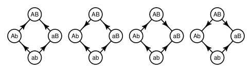
Figure 1. The arrows point toward the more fit genotype. The graphs represent no sign epistasis, two cases with sign epistasis but not reciprocal sign epistasis, and one case with reciprocal sign epistasis.

Sign epistasis is by no means rare for microbes according to several studies (e.g. Desper et al.,, 1999; Weinreich et al.,, 2005, 2006; Beerenwinkel et al., 2007 a, ; Franke et al.,, 2011; Szendro et al.,, 2013; Goulart et al.,, 2013). In particular, sign epistasis occurs for antibiotic resistance mutations, as well as for HIV and malaria. In fact, existing studies suggest that absence of sign epistasis is exceptional for systems associated with drug resistance for $L\geq 4$.

Sign epistasis is of clinical importance for several reasons. A recent approach for preventing and managing resistance problems takes advantage of both sign epistasis and variable selective environments (Goulart et al.,, 2013). Another aspect of managing drug resistance is to find constraints for orders in which mutations accumulate from genotype data (Desper et al.,, 1999; Beerenwinkel et al., 2007 a, ). A constraint could be that a particular mutation is selected for (meaning that that the mutation is beneficial) only if a different mutation has already occurred. The existence of constraints implies sign epistasis. Indeed, if a particular mutation is beneficial regardless of background, then it can occur before or after other mutations. Moreover, sign epistasis is relevant for predictions of how populations will adapt (Weinreich et al.,, 2006).

Fitness graphs are useful for the empirical problems mentioned, as well as for more theoretical problems, including the relation between global and local properties of fitness landscapes (see Section 3). If one can order a set of genotypes by decreasing fitness, one has determined the fitness ranks. More fine scaled information, such as relative fitness values, may not be known. A fitness graph compares the fitness ranks of mutational neighbors. For simplicity, whenever we use fitness graphs we assume that $w_{s}\neq w_{s^{\prime}}$ for any two strings $s$ and $s^{\prime}$ which differ in one position only.

Roughly, consider the zero-string as the starting point (possibly the wild-type), and each non-zero position of a string as an event, i.e., that a mutation has occurred. Under these assumptions the fitness graph coincides with the Hasse-diagram of the power set of events, except that each edge in the Hasse-diagram is replaced with an arrow toward the string with greater fitness.

For a formal definition, a fitness graph is a directed graph where each node corresponds to a string of $\Sigma^{L}$. The fitness graphs has $L+1$ levels. Each string such that $\sum s_{i}=l$ corresponds to a node on level $l$ in the fitness graph. In particular, the node representing the zero-string is at the bottom, the nodes representing strings with exactly one non-zero position, including $10\cdots 0,$ are one level above, the nodes representing strings with exactly two non-zero positions, including $110\cdots 0,$ are on the next level, and the 1-string is at the top. Moreover, the nodes are ordered from left to right according to the lexicographic order where $1>0$ of the corresponding strings (see e.g. Fig. 5). A directed edge connects each pair of nodes such that the corresponding strings differ in exactly one position. The edge is directed toward the node representing the more fit of the two genotypes.

Remark 1.

Unless otherwise stated, the words ”level”, ”up”, ”down” ”above” and ”below” refer to fitness graphs. In particular, notice that a higher level does not imply greater fitness.

For $L\geq 2$, given a string and two positions, consider the four strings which coincide with the original string except in (at most) the two positions. We call the strings a type 2 system if there is reciprocal sign epistasis, a type 1 system if there is sign epistasis, but not reciprocal sign epistasis, and a type 0 system if there is no sign epistasis.

For interpretations of general fitness graphs, it may be helpful to first analyze the two-loci case shape in some detail. There exist exactly 14 fitness graphs for biallelic two-loci systems (see Fig. 2), where 4 are type 0 systems, 8 type 1 systems, and 2 type 2 systems. One verifies the following result.

Remark 2.

For two-loci, type 0, 1, and 2 systems have the following properties:

1. A type 0 system can be rotated so that all arrows point up.

2. A type 1 system differs from a cycle by exactly one arrow.

3. A type 2 system have two nodes such that all edges are directed toward them, and two nodes such that no edges are directed toward them.

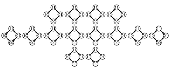
Figure 2. For a fitness graph, the arrows point toward the genotype of greater fitness. There exist exactly 14 fitness graphs for biallelic two-loci systems, where the type 0 systems are on the first row, the type 1 systems on the second row, and the type 2 systems on the third row.

The observations from the two-loci case should make it easy to identify type 0, 1 and 2 systems for general fitness graphs. Fig. 3 and 4 show fitness graph for 3-loci systems. Fig. 3a has type 0 systems only, Fig. 3b type 0 and 2 systems, Fig. 4a type 0, 1 and 2 systems, and Fig. 4b type 2 systems only. Fig. 5 shows a fitness graph for a 4-loci population, where there are several type 2 systems, including 0001, 0101, 0011, 0111.

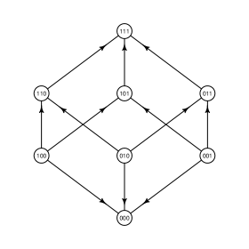
Figure 3. A fitness graph shows sign epistasis and the peaks. The graph in Fig. 3a has type 0 systems only. The graph in Fig. 3b has type 0 and type 2 systems, but no type 1 systems.

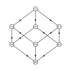
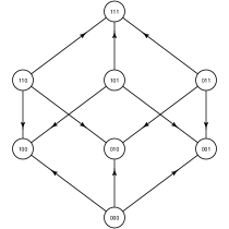
Figure 4. The graph in Fig. 4a has type 0, type 1 and type 2 systems. The graph in Fig. 4b has type 2 systems only, and the corresponding fitness landscape has four peaks.

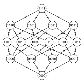
Figure 5. The fitness landscape has peaks at $1100$, $0011$ and $1111$, whereas all triple mutants (mutants on the third level) have low fitness

3. Fitness graphs and theoretical results

Fitness graphs have mostly been used in empirical work (e.g. De Visser et al.,, 2009; Franke et al.,, 2011; Szendro et al.,, 2013; Goulart et al.,, 2013). However, we will indicate how they can be used in theoretical arguments, and mention some results where the proofs depend on fitness graphs.

It is known that one can have $2^{L-1}$ peaks in a fitness landscape (e.g. Haldane,, 1931) and this number is an upper bound. The proof is elementary, and we will not give the details. However, we will construct fitness landscapes with the maximal number of peaks using fitness graphs.

Example 1.

For any $L$, consider the fitness graph where the edges are directed up from level 0 to 1, down from level 1 to 2, up from level 2 to 3, and so on. The fitness graph in Fig. 4b is an example. Notice that the graph corresponds to fitness landscapes with 4 peaks, i.e., the maximal number of peaks for $L=3$. In general, all nodes at level $1,3,5\dots$ are at peaks, and such fitness graphs correspond to fitness landscapes with exactly $2^{L-1}$ peaks.

Recent work relates global and local properties of fitness landscapes (Poelwijk et al.,, 2007, 2011; Crona et al., 2013 a, ). This topic is of interest, since most empirical studies of fitness landscapes concern local properties, including sign epistasis. It has been shown that multipeaked fitness landscapes have type 2 systems (Poelwijk et al.,, 2011). The converse is not true. However, a sufficient condition for multiple peaks can be phrased in terms of type 1 and 2 systems. More precisely, the following result was proved using fitness graphs.

1.

(Crona et al., 2013) If a fitness landscape has type 2 systems and no type 1 systems, then it has multiple peaks.

It follows that the landscapes corresponding to Fig. 3b and 4b have multiple peaks.

Fitness graphs are efficient for analyzing mutational trajectories. We will state a result regarding accessible mutational trajectories from Weinreich et al., (2005). A brief proof of the result using fitness graphs was given in Crona et al., 2013 a , but the original proof does not use fitness graphs.

We call the global maximum of the landscape ”the fitness peak”. Moreover, define a general step similar to ”adaptive step”, except that the fitness may decrease. A general walk, as opposed to an ”adaptive walk” is a sequence of general steps. If a general walk between two nodes has minimal length, we call it a shortest walk.

2.

(Weinreich et al., 2005)

1. The following conditions are equivalent for a fitness landscape.

   1. Each general step toward the fitness peak, i.e., a step that decreases the graph theoretical distance to the peak, is an adaptive step.

   2. Each shortest general walk to the fitness peak is an adaptive walk.

   3. The fitness landscape has no type 1 or 2 systems.

2. If the equivalent conditions in (1) are satisfied, then each adaptive walk to the fitness peak is a shortest general walk.

A fitness landscape satisfying the equivalent conditions (i)–(iii) above is referred to as a fitness landscape lacking genetic constraints on accessible mutational trajectories in Weinreich et al., (2005). For $L=3$, the fitness graph in Fig. 3a corresponds to this category of landscapes. Fitness landscapes lacking genetic constraints on accessible mutational trajectories can be represented by fitness graphs where all arrows are up. For brevity, we will refer to ”all arrows up landscapes”.

It is important to notice that the concept of an all arrows up landscape is biologically meaningful. Even if a landscape is single peaked, type 1 systems may cause the adaptation process to be slower since not all shortest general walks to the peak are adaptive walks. However, for all arrows up landscapes, there are no local obstacles for the adaptation process.

4. Fitness graphs and recombination

Recombination can generate new genotypes in a population. Under some circumstances, recombination will speed up adaptation. An early hypothesis about the possible advantage of recombination concerned double mutants of high fitness, where the corresponding single mutations are deleterious. It was suggested that recombination could generate such double mutants. In terms of fitness graphs this case can be described as a type 2 system, where the wild-type is at a fitness peak. However, the hypothesis was immediately criticized, and described as a ”widespread fallacy” by Muller (Crow,, 2006). The two single mutations being deleterious, it seems unlikely that the the corresponding genotypes would appear and recombine to the double mutant. The (current) consensus is that under most circumstances recombination will not be of any use in the situation described, i.e., for a two-loci type-2 system, where the wild-type is at a peak (see also Lenski et al., (2003)). However, using fitness graphs we will argue that recombination could be an advantage in somewhat related cases where $L\geq 3$.

The topic of recombination is involved with subtle differences between effects on the population level and the gene level. For instance, it is theoretically possible that recombination is beneficial for a population and at the same time recombination suppressors could be selected for (see e.g. Otto and Lenormand, (2002) for comments and references). We do not intend to develop new theory, or describe existing knowledge of recombination in any detail. For an overview of the field, we refer to Otto and Lenormand, (2002). Our goal is to point out mechanisms specific for $L\geq 3$ loci which should be considered for an analysis of the effect of recombination. This is justified since the field is dominated by work in the two-loci case, or mechanisms which can be reduced to the two-loci case.

It has been suggested that recombination has an especially strong impact in structured populations (see e.g. Martin et. al,, 2006). A populations is structured, as opposed to well mixed, if the genotype frequencies varies between geographic locations. In particular, if a population is subdivided into local subpopulations with some migration between them, then recombination could be advantageous.

We will sketch a model within this framework, which we call a puddles and flood population. We mainly have microbes in mind, for example bacteria. Assume that the local subpopulations live in puddles, and the subpopulations are homogeneous for most of the time. Occasionally, there is a flood where the contents of the local puddles get thoroughly mixed. After a flood, life proceeds as usual in the puddles for an extended period, until the next flood. Under these assumptions, genotypically different subpopulations are likely to mix, so that recombination can generate new genotypes.

Example 2.

Consider the fitness graph in Fig. 5, and assume that 0000 is the wild-type. Both 1100 and 0011 are at peaks, whereas the triple mutants are less fit as compared to adjacent double mutants. For a puddles and flood population, recombination of double mutants may result in 1111. In this case recombination could speed up adaptation.

Notice that in the absence of recombination, one could obtain 1111 from 1100, only if there is a double mutation, since the triple mutants are not fit.

Example 3.

Consider the fitness graph in Fig. 4b. Assume that 000 is the wild-type. From the fitness graph, the single mutants 100, 010, 001 are at peaks. Under the assumption that 111 has maximal fitness, recombination could speed up adaptation. However, two recombination events are necessary. For instance, recombination of 100 and 010 could result in 110. Then recombination of 110 and 001 could result in 111.

Notice that there is an important difference between Examples 2 and 3. For instance, consider the outcome for a puddles and flood population where no more than two puddles mix at the time. Then one could obtain 1111 by recombination in Example 2. Indeed, if an 1100 population and an 0011 population mix, recombination could produce the 1111 genotype.

In contrast, consider Example 3 under the same restriction (no more than two puddles mix). If say an 100 and 010 population mix, one could obtain 110 by recombination. However, 110 is selected against so that 111 is unlikely to appear under most circumstances. (On the other hand, if several puddles mix, one could get a mixture of the single mutants 100, 010 and 001, and recombination could result in 111).

Consider all arrows up fitness landscapes where the 1-string has maximal fitness. Then one could obtain the 1-string from a sequence of single mutations. However, for a puddles and flood population, recombination could speed up adaptation. This is because the process of accumulating $L$ single mutations could be time consuming.

Example 4.

For an all arrows up $L$-loci fitness landscape where considerably more than $L$ puddles tend to mix during a flood period, one could obtain the 1-string already after one flood period.

The examples described are theoretical constructions. It is not obvious if Examples 2 and 3, or similar cases, occur frequently enough in nature for having much of an impact. A first question to ask for a population, is how frequently it happens that ”good+good=not good” for single mutations. This type of problems is the topic for the next section.

5. Fitness graphs and other qualitative measures

In order to determine if one has a reasonable chance to find fitness graphs of the types described in the previous sections, the following qualitative concept (Crona et al., 2013 a, ) may be useful.

We define $B$ and $B_{p}$ as follows. The set $B_{p}$ consists of all double mutants such that both corresponding single mutations are beneficial.

The set $B\subseteq B_{p}$ consists of all double mutants in $B_{p}$ which are more fit than at least one of the corresponding single mutants.

The qualitative measure of additivity for a fitness landscape is the ratio $\frac{|B|}{|B_{p}|}$. Notice that $\frac{|B|}{|B_{p}|}=1$ for all arrows up landscapes.

Fitness landscapes are defined as additive if fitness effects of mutations sum. For example, if

$$w_{00}=1,w_{10}=1.2,w_{01}=1.3,$$

then additive fitness implies that $w_{11}=1.5$ (since $0.5=0.2+0.3$, so that the fitness effects of two mutations sum). Notice that fitness is additive exactly if

$$w_{11}-w_{10}-w_{01}+w_{00}=0\,.$$

By definition, fitness is additive exactly if there is no epistasis. One may consider all arrows up landscapes as the qualitative correspondence to additive fitness landscapes.

Antibiotic resistance landscapes for a particular 4-loci system and 9 selective environments were studied in Goulart et al., (2013). More precisely, all combination of the TEM-1 mutations L21F, R164S, T265M and E240K were considered. The length of TEM-1 is 287, i.e., TEM-1 can be represented as a sequence of 287 letters in the 20-letter alphabet corresponding to the amino acids. The notation L21F means that the amino acid Leucine (L) at position 21 has been replaced by the amino acid Phenylalanine (F). The mutations R164S, T265M and E240K are defined similarly, using the standard notation for amino acids. The mean value of $\frac{|B|}{|B_{p}|}$ for the 9 selective environments was 0.57.

In contexts where the relative fitness values of genotypes are not known, qualitative concepts can still be used. It is valuable to understand qualitative information for several reasons. Fitness ranks tend to be easier to determine as compared to relative fitness, and from records of mutations one can sometimes draw conclusions about fitness ranks without making measurements. We argue that much can be learned about fitness landscape from existing records of mutations, in particular from drug resistance mutations. However, one needs to be able to interpret qualitative information, a theme developed in Crona et al., 2013 b with applications to antibiotic resistance, see also Crona et al., 2013 a .

The qualitative measure of additivity is coarse. If relative fitness values can be determined, one may want to consider quantitative fitness differences as well. For a quantitative measure of additivity, we refer to the concept ”roughness” (Carnerio and Hartl,, 2010; Aita et al.,, 2001). Briefly, additive fitness landscapes have roughness 0, and any deviation from additivity implies that the roughness is greater than 0.

6. Shapes

Throughout the remainder of the chapter, we consider biallelic $L$-loci populations, where we assume that all $2^{L}$ genotypes occur in the populations (for a comment regarding this simplification, see Section 10), and a fitness landscape

$$w:\Sigma^{L}\mapsto\mathbb{R},\,\Sigma=\{0,1\}.$$

Moreover, for $L=2\text{ and }3$ we use the following orders of the genotypes (from left to right):

$$00,01,10,11\text{ and }000,001,010,011,100,101,110,111.$$

Most empirical studies of epistasis for several loci focus on the average curvature (Fig. 6) or pairwise gene interactions using ANOVA methods (Beerenwinkel et al., 2007 b, ). For beneficial mutations, antagonistic epistasis means that the combined effect of mutations are less than the sum of individual effects, whereas synergistic epistasis means that the combined effect of mutations exceeds the sum of individual effects. It has been claimed that antagonistic epistasis dominates for beneficial mutations in nature (e.g. Kryazhimskiy et al.,, 2011). Antagonistic and synergistic epistasis are defined analogously for deleterious mutations (Fig. 6). A motivation for the interest in average effects of mutations is the connection to recombination. According to standard models, antagonistic epistasis for beneficial mutations sometimes implies an advantage for recombination (Otto and Lenormand,, 2002).

Figure 6. The number of mutations increases along the horizontal axis, and the fitness increases along the vertical axis. For Fig. 6a, the mutations are beneficial. The upper curve corresponds to antagonistic epistasis, and the lower curve to synergistic epistasis. For Fig. 6b, the mutations are deleterious. The upper curve corresponds to synergistic epistasis and the lower curve to antagonistic epistasis.

Conventional summary statistics for epistasis have their limitations. The average curvature may obscure a diversity of interaction types, and pairwise tests fail to discover curvature at genetic distances greater than two. The most fine-scaled approach to gene interactions is the geometric theory, introduced in Beerenwinkel et al., 2007 b . The theory reveals all the gene interactions, and it depends on triangulations of polytopes. For mathematical background we refer to De Loera et al., (2010), see also Ziegler, (1995) for the general theory about polytopes. The geometric approach has revealed previously unappreciated gene interactions for HIV, Escherichia-coli and in some other cases (Beerenwinkel et al., 2007 b, ; Beerenwinkel et al., 2007 c, ), and the approach is relevant for recombination.

We will start with an informal introduction to the geometric theory, where the main purpose is to provide an intuitive understanding and some geometric interpretations. More formal descriptions are given in the next sections.

Roughly, a triangulation of a polygon is a subdivision of the polygon into triangles. A triangulation of the $L$-cube is a subdivision of the cube into simplices (triangles if $L=2$, tetrahedra if $L=3$, pentachora for $L=4$, and so on). We will use some concepts which are defined in terms of populations. If one groups individuals into classes of identical genotypes, a population can be described as the frequencies of the genotypes. The fitness of a population is defined as the average fitness of all individuals.

First consider the case $L=2$. Let

$$\Delta=\{(p_{00},p_{01},p_{10},p_{11})\in[0,1]^{4}\,:\,p_{00}+p_{01}+p_{10}+p_{11}=1\}$$

denote the population simplex. A population is given as a point in $\Delta$. The genotope for $L=2$ is the square with vertices $00,01,10,11$. We denote this genotope $[0,1]^{2}$, and interpret a point $v=(v_{1},v_{2})\in[0,1]^{2}$ as the allele frequencies of the population, where $v_{1}$ denotes the frequency of 1’s at the first locus, and $v_{2}$ the frequency of 1’s at the second locus.

For a simple example, consider a population where half of the individuals have genotype 00, and the other half 11. Then the allele frequency vector is $(0.5,0.5)$. For a population where half of the individuals have the genotype 01 and the other half 10, the allele frequency vector is $(0.5,0.5)$ as well. However, the average fitness may differ between the two populations.

We will analyze examples in more detail.

Example 5.

Consider $v=(0.4,0.8)\in[0,1]^{2}$ and the populations $p^{1}=(0.2,0.4,0,0.4)\in\Delta$ and $p^{2}=(0,0.6,0.2,0.2)\in\Delta$. One verifies that both populations have the allele frequencies described by $v$; indeed, adding the contributions of 1’s for $p^{1}$ and the first locus gives $0+0.4=0.4$, and for the second locus $0.4+0.4=0.8$. The contributions for $p^{2}$ gives $0.2+0.2=0.4$ for the first locus, and $0.6+0.2=0.8$ for the second.

Let $\rho$ denote a corresponding map from the population simplex $\Delta$ to the genotope $[0,1]^{2}$, where

$$\rho(p_{00},p_{01},p_{10},p_{11})=\left(p_{10}+p_{11},p_{01}+p_{11}\right).$$

Then $\rho$ maps a point of the population simplex to the allele frequencies, where $p_{10}+p_{11}$ equals the frequency of 1’s at the first locus, and $p_{01}+p_{11}$ equals the frequency of 1’s at the second locus. Notice that $\rho(p^{1})=\rho(p^{2})=v$ in the previous example.

Given a fitness landscape and a vector $v\in[0,1]^{2}$, a fittest population $p\in\Delta$ has maximal fitness among populations such that the allele frequencies are described by $v$. Moreover, $p$ is unique for $L=2$, except in the case when fitness is additive (see also the comment after Case 2 below). For a fittest population, one cannot increase the fitness by shuffling around alleles. The biological significance is immediate, since such allele shuffling relates to recombination.

For a geometric interpretation, the fitness landscapes $w$ (usually) induces a triangulation of the genotope $[0,1]^{2}$. This triangulation is the shape of the fitness landscape. The critical property of the triangulation is that for $v\in[0,1]^{2}$, the genotypes that occur in the fittest population are the vertices of the triangle which contains $v$. The corresponding result holds for any $L$. We will first describe the triangulations, and then give a geometric interpretation of shapes. As remarked, fitness is additive exactly if

$$w_{11}-w_{10}-w_{01}+w_{00}=0\,.$$

For simplicity, we call the case where 11 has higher fitness as compared to a linear expectations positive epistasis, and similarly for negative epistasis.

Case 1: (positive epistasis) If

$$w_{11}-w_{10}-w_{01}+w_{00}>0,$$

then the triangulation induced by the fitness landscape has $00-11$ diagonal, meaning that the triangles are $\{00,01,11\}$ and $\{00,10,11\}$ (Fig. 7).

Case 2: (negative epistasis) If

$$w_{11}-w_{10}-w_{01}+w_{00}<0,$$

then the induced triangulation of the genotope has $10-01$ diagonal meaning that the triangles are $\{00,01,10\}$ and $\{01,10,11\}$ (Fig. 7).

For positive epistasis, $p^{1}$ in Example 5 is a fittest population. Indeed, positive epistasis implies that whenever one replaces 10 and 01 genotypes by 00 and 11 genotypes, the result is increased average fitness of the population. However, for $p^{1}$ the proportions of 00 and 11 genotypes are maximal (in the sense that one cannot replace 10 and 01 genotypes by 00 and 11 genotypes), so that $p^{1}$ has maximal fitness given the allele frequency vector $v=(0.4,0.8)$.

For positive epistasis, notice that $v=(0.4,0.8)$ is a point in the triangle $\{00,01,11\}$ and that the genotypes of $p^{1}$ are 00,01, 11. Moreover, 10 and 01 are not on the same triangle, which indicates that one can increase fitness by replacing them with other genotypes. These observations illustrate how shapes and fittest populations relate for $L=2$.

For a geometric interpretation of shapes, consider the genotope $[0,1]^{2}$ and the four points above the vertices of $[0,1]^{2}$, such that the height coordinates correspond to fitness. The four points are vertices of a tetrahedron (Fig. 7). The upper sides of the tetrahedron (marked with different patterns) project onto two triangles of $[0,1]^{2}$. The projections describe the triangulation induced by $w$. The left picture corresponds to positive epistasis, and the right to negative epistasis. This construction should make sense, since the triangulation obtained as projections of the upper faces of the tetrahedron has the critical property for all fittest populations. More precisely, for any $v\in[0,1]^{2}$, a fittest population consists of vertices of the triangle which contain $v$. The fitness landscape almost always induces a triangulation of the genotope $[0,1]^{2}$ as described. Such a triangulation is a generic shape. The exceptional (non-generic) case is when fitness is additive.

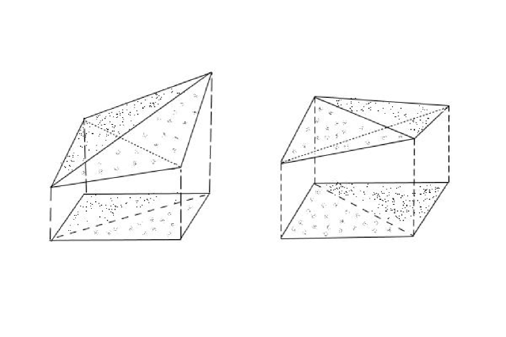
Figure 7. The upper pictures show the triangulations of the genotopes (the squares) in Case 1 (positive epistasis) and 2 (negative epistasis). The lower left picture shows the tetrahedron above the genotope in Case 1, where the height coordinates correspond to the fitness of the four genotypes under consideration. The projections of the upper sides of the tetrahedron describe the triangulations. The lower right picture shows how the triangulation is induced in Case 2.

In general, consider a biallelic $L$-loci system and the fitness landscape $w$. The genotope is the $L$-cube $[0,1]^{L}$, where the vertices represent the genotypes. As in the two-loci case, let $\Delta$ denote the population simplex and let $\rho$ denote the corresponding map from $\Delta$ to $[0,1]^{L}$. For a fixed $v\in[0,1]^{L}$, consider the linear programming problem

$$\max\,\{\,p\cdot w:\rho(p)=v\}.$$

A solution gives the maximal population fitness, i.e., the maximum of $p\cdot w$, given the allele frequency vector $v$ (since $\rho(p)=v)$. Consequently, finding the fittest population translates to solving this linear programming problem.

If we let $v$ vary, we get the following parametric linear programming problem

$$\tilde{w}(v)=\max\{\,p\cdot w:\rho(p)=(v){\text{ for all }}v\in[0,1]^{L}\}.$$

The domains of linearity of $\tilde{w}$ do almost always constitute a triangulation of the genotope (De Loera et al.,, 2010, Chapter 2). The shape of the fitness landscape is the triangulation of $[0,1]^{L}$ induced by the fitness landscape $w$. The geometric interpretation is analogous to the two-loci case, so that the triangulation is obtained as the projections of the upper faces of the polytope constructed from the fitness landscape. Moreover, in the generic case, i.e., if the shape of the fitness landscape is a triangulation, the fittest population is unique for a given allele frequency vector $v$. More precisely, the genotypes that occur in the fittest population are the vertices of the simplex which contains $v$.

For the two-loci case, the geometric theory does not contribute anything new, since there exist only two triangulations corresponding to the two types of epistasis in the usual sense. However, for $L=3$, there are 74 generic shapes corresponding to triangulations of the cube (see Section 9).

Not all triangulations can be obtained from a fitness landscape. A triangulation is regular if it is induced by some fitness landscape. Fig. 8 shows a non-regular triangulation. This is the smallest non-regular triangulation.

Figure 8. A non-regular triangulation. This triangulation cannot be induced from a fitness landscape.

In the literature, a regular triangulation is described as a triangulation which is induced by a cost vector. Then the linear programming problem concerns minimizing the cost, and the triangulations are obtained as projections of all lower faces of the polytope constructed from the cost vector. Since our topic is fitness landscapes, we think in terms of maximal fitness rather than minimal costs.

7. Shapes and flips

For $L>2$, there are many possible shapes. It may seem that shapes are difficult to apply in empirical biology, due to ambiguity from measurement errors. However, the geometric theory comes with a structure. Shapes may be similar or completely different, and the relation between shapes can be described in a systematic way. We start with intuitive descriptions. Briefly, a flip, sometimes referred to as a geometric bistellar flip, is a minimal change between triangulations. Fig. 9, 10 and 11 show flips. For the two-loci case, the two triangulations corresponding to positive and negative epistasis differ by a flip.

For an overview of how all triangulations of a polytope are related, one can consider the flip graph. The nodes of the graph are the triangulations, and edges connect triangulations which differ by a flip. Fig. 12. shows the flip graph of a hexagon. The graph theoretical distance between triangulations can be considered a measure of how closely related the triangulations are. Some caution is necessary if one is primarily interested in regular triangulation, since a regular triangulation may be transformed into a non-regular triangulation by a flip.

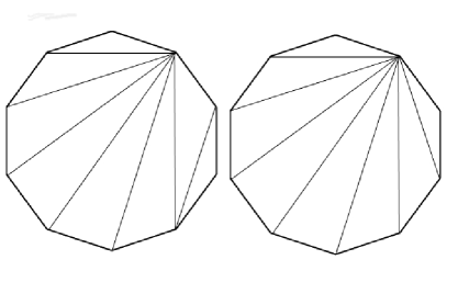
Figure 9. The left triangulation can be transformed into the right triangulation by a flip.

Figure 10. The dashed lines indicate the triangulations. The triangulations differ by a flip.

Figure 11. The triangulations differ by a flip, and the number of triangles are different for the two triangulations.

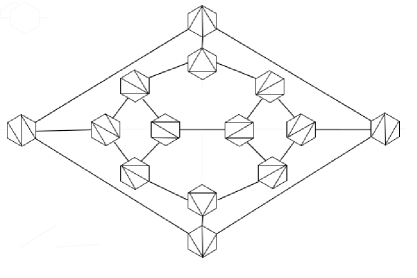
Figure 12. The flip graph of a hexagon.

8. Shapes and polyhedral subdivisions

Given a genotype space $\Sigma^{L}$, consider all possible shapes induced by fitness landscapes $w:\Sigma^{L}\mapsto{\mathbb{R}}.$ We will describe how the shapes are related. Most results depend on triangulations of polytopes. In particular, we will discuss the secondary polytope (Gelfand et al.,, 1994), an important construction in discrete mathematics. The secondary polytope is useful for a global understanding of shapes. We will not provide proofs, but rather describe results and how they apply to epistasis. For a thorough treatment, including proofs, see De Loera et al., (2010) and for the biological perspective Beerenwinkel et al., 2007 b . Remark 3 in the end of Section 9 explains how our applications relate to the general theory about polytopes. Some definitions below may seem technical, but the figures and intuitive descriptions from the previous sections should help.

Throughout the section, let ${\bf{A}}\in{\mathbb{R}}^{d}$ denote a finite point set. A polytope is the convex hull of a point set, and $\text{conv}({\bf{A}})$ denotes the convex hull of ${\bf{A}}$.

Polytopes include points, line segments, triangles and tetrahedra, as well as $L$-cubes and polygons. We will use some concepts expressed in terms of point sets, although we have polytopes in mind. In particular, a triangulation of a polytope is a triangulation of the set of its vertices, and similarly for the other concepts.

A $k$-simplex is the convex hull of $k+1$ affinely independent points. In particular, points, segments, triangles and tetrahedra are simplices.

A j-face of a $k$-simplex is the convex hull of a subset of $j$ vertices.

We will give a formal definition of triangulations and some related concepts. A polyhedral subdivision of a point set ${\bf{A}}$ is a collection of polytopes $\mathcal{C}$, such that

1. If $C\in\mathcal{C}$ then each face of $C$ belongs to $\mathcal{C}$ as well (closure property),

2. the union $\cup_{C\in\mathcal{C}}C=\text{conv}({\bf{A}})$ (union property),

3. for $C\neq C^{\prime}$ where $C,C^{\prime}\in\mathcal{C}$, the intersection $C\cap C^{\prime}$ does not contain any interior points of $C$ or $C^{\prime}$ (intersection property).

A triangulation of ${\bf{A}}$ is a polyhedral subdivision such that all polytopes are simplices. A refinement $\mathcal{C^{\prime}}$ of a polyhedral subdivision $\mathcal{C}$ is a polyhedral subdivision $\mathcal{C^{\prime}}$ where for each $C^{\prime}\in\mathcal{C^{\prime}}$, there exists a $C\in\mathcal{C}$, such that $C^{\prime}\subset C$. A polyhedral subdivision is an almost triangulation if it is not a triangulation, but all its proper refinements are triangulations. Two triangulations of the same point set are connected by a flip if they are the only two triangulations refining an almost triangulation. All these concepts are illustrated in Fig. 9 and 13. Specifically, Fig. 13 shows a polyhedral subdivision which is also an almost triangulation. Moreover, the two possible refinements are the triangulations in Fig. 9. As mentioned, the triangulations in Fig. 9 differ by a flip, so that the formal definition agrees with the descriptions in the previous section.

Figure 13. The polyhedral subdivision is an almost triangulation. The two possible refinements result in the two triangulations from Fig. 9.

From the previous section, a triangulation induced by the fitness landscape is the shape of the landscape. More generally, we can describe all shapes using the concepts defined in this section. Consider again the parametric linear programming problem where $v$ varies:

$$\tilde{w}(v)=\max\{\,p\cdot w:\rho(p)=(v){\text{ for all }}v\in[0,1]^{L}\}.$$

The domains of linearity of $\tilde{w}$ constitute a polyhedral subdivision (De Loera et al.,, 2010, Chapter 2) of the genotope. The shape of a fitness landscape is the polyhedral division induced by the landscape. This subdivision is not always a triangulation. Recall from the two-loci case that positive epistasis corresponds to $u>0$ and negative epistasis to $u<0$, for

$$u=w_{00}-w_{01}-w_{10}+w_{11}.$$

However, one does not obtain a triangulation if $u=0$. As remarked, the fitness landscape is generic if it induces a triangulation, and the corresponding shapes are the generic shapes.

In order to further describe the relations between shapes, we will consider minimal dependence sets of points, as in the following example.

Example 6.

Consider the vertices of the genotope $[0,1]^{2}$. The relation

$$1\cdot(0,0)-1\cdot(0,1)-1\cdot(1,0)+1\cdot(1,1)=0,$$

is an affine dependence relation, since the sum of the coefficients $1-1-1+1$ is zero. This set of four points is a minimal dependence set, in the sense that every proper subset of the four points is independent. The form

$$w_{00}-w_{01}-w_{10}+w_{11},$$

corresponds to the dependence relation. Notice that the form is unique up to scaling, i.e., multiplication by a constant.

We define a circuit as a minimal affine dependence set. The corresponding forms are called circuits as well, and they are unique up to scaling. Flips and circuits are closely related. The circuit $u$ corresponds to the flip between the two triangulations of the genotope in the two-loci case. More precisely, the triangulation corresponding to positive epistasis is described by $u>0$, and the flip corresponds to replacing $u>0$ by $u<0$. In general, a flip corresponds to changing sign of a circuit, and some examples for $L=3$ are given in the next section. The next concept will be used for defining the secondary polytope, and for describing flips and circuits in more detail.

For a triangulation of a polytope, we define the GKZ vector as follows: Each component of the GKZ vector corresponds to a vertex of the polytope. The component is the sum of the normalized volumes of all simplices containing the vertex.

In this context, it is sufficient to use that the normalized volume of the $L$-cube $[0,1]^{L}$ is $n!$, so that the genotope $[0,1]^{2}$ in the two loci case has area 2, and the genotope $[0,1]^{3}$ in the 3-loci case has volume 6. In general, for an n-dimensional lattice polytope, the normalized volume is defined as the Euclidean volume of the polytope multiplied by $n!$

Example 7.

The GKZ-vector for the triangulation of $[0,1]^{2}$ in the two-loci case associated with positive epistasis is $(2,1,1,2)$, using the order as given in the beginning of Section 6. Indeed, both triangles have area 1 (using normalized volumes). The vertices $00$ and $11$ belong to two different triangles each, whereas $10$ and $01$ are ”sliced off”, so that each of them belong to one triangle only. Similarly, the GKZ-vector for the triangulation associated with negative epistasis is $(1,2,2,1)$.

The purpose with the next example is to relate circuits and GKZ vectors.

Example 8.

From the previous example, the GKZ-vector for the triangulation associated with positive epistasis is $(2,1,1,2)$, whereas the the GKZ vector for the triangulation associated to negative epistasis is $(1,2,2,1)$. We relate to the circuit $u=w_{00}-w_{01}-w_{10}+w_{11}$ the vector $(1,-1,-1,1)$. The flip between the two triangulations corresponds to $u$, and

$$(2,1,1,2)-(1,2,2,1)=(1,-1,-1,1)$$

so that the GKZ vectors differ by the vector corresponding to the circuit associated with the flip.

See Remark 3 for some comments about the relation between GKZ vectors and flips, including references. In the next section, we will consider the relations between flips and GKZ vectors for $L=3$.

For a given polytope the secondary polytope is defined as the the convex hull of the GKZ vectors. The geometric classification of fitness landscapes depends on the secondary polytope. For a genotope, the vertices of the secondary polytope correspond to generic shapes, and its edges to flips between the generic shapes. The higher dimensional faces of the secondary polytope correspond to non-generic shapes. Consequently, the secondary polytope represent all the shapes and their relations.

Example 9.

The secondary polytope for the two-loci case is a line segment, where the vertices corresponds to the two triangulations, and the line segment to the flat shape.

9. The 74 generic shapes of the cube

The relations between shapes, circuits and GKZ vector for the 3-cube, is analogous to the two-loci case, as indicated in the previous section. Recall that the square has 2 generic shapes, corresponding to $u>0$ and $u<0$, for

$$u=w_{00}-w_{01}-w_{10}+w_{11}.$$

The cube has 74 generic shapes, where a shape is determined by the following 20 circuits:

$$a :=w_{000}-w_{010}-w_{100}+w_{110}$$

$$b :=w_{001}-w_{011}-w_{101}+w_{111}$$

$$c :=w_{000}-w_{001}-w_{100}+w_{101}$$

$$d :=w_{010}-w_{011}-w_{110}+w_{111}$$

$$e :=w_{000}-w_{001}-w_{010}+w_{011}$$

$$f :=w_{100}-w_{101}-w_{110}+w_{111}$$

$$g :=w_{000}-w_{011}-w_{100}+w_{111}$$

$$h :=w_{001}-w_{010}-w_{101}+w_{110}$$

$$i :=w_{000}-w_{010}-w_{101}+w_{111}$$

$$j :=w_{001}-w_{011}-w_{100}+w_{110}$$

$$k :=w_{000}-w_{001}-w_{110}+w_{111}$$

$$l :=w_{010}-w_{011}-w_{100}+w_{101}$$

$$m :=w_{001}+w_{010}+w_{100}-w_{111}-2w_{000}$$

$$n :=w_{011}+w_{101}+w_{110}-w_{000}-2w_{111}$$

$$o :=w_{010}+w_{100}+w_{111}-w_{001}-2w_{110}$$

$$p :=w_{000}+w_{011}+w_{101}-w_{110}-2w_{001}$$

$$q :=w_{001}+w_{100}+w_{111}-w_{010}-2w_{101}$$

$$r :=w_{000}+w_{011}+w_{110}-w_{101}-2w_{010}$$

$$s :=w_{000}+w_{101}+w_{110}-w_{011}-2w_{100}$$

$$t :=w_{001}+w_{010}+w_{111}-w_{100}-2w_{011}$$

We will use the letters $a-t$ in the list, as well as $u$, throughout the section.

In order to emphasize the connection to gene interactions, especially the algebraic aspects of epistasis, we will consider the interaction space. For any $L$, let $\mathcal{L}$ be the subspace of ${\mathbb{R}}^{\Sigma^{L}}$ consisting of additive fitness landscapes. The interaction space is the vector space dual to the quotient of ${\mathbb{R}}^{\Sigma^{L}}$ modulo $\mathcal{L}$, or

$${\left({\mathbb{R}}^{\Sigma^{L}}/\mathcal{L}\right)}^{\ast}.$$

The interaction space is spanned by the set of all circuits, where the circuits are unique up to scaling. In the two-loci case, the interaction space is spanned by $u$. For $L=3$, the interaction space is spanned by the 20 circuits $a-t$.

The circuit sign pattern of a fitness landscape consists of the sign (positive, negative or zero) of each circuit. In the two-loci case there is only one circuit and the sign pattern is either $u>0$, $u<0$ or $u=0$. A central result for the geometric classification is that the circuit sign pattern determines the shape of the fitness landscape, but in general the converse does not hold (Beerenwinkel et al., 2007 b, ). In particular, the signs of the 20 circuits $a-t$ determine the shape of the fitness landscape for $L=3$. In total, there are 74 generic shapes. The fact that there are 20 circuits and only 74 generic shapes reflects dependence relations.

Table 1 lists the shapes, where the vertices of the cube are ordered as follows

$$000,001,010,011,100,101,110,111.$$

Table 1. Shape numbers, GKZ vectors, inequalities and adjacent shapes

$\#$	GKZ	inequalities	$\#$	GKZ	circuits
1	15515115	tqom3,4,5,6	38	31355313	$\overline{\text{l}}\overline{\text{g}}$cd39,44,51,59
2	51151551	srpn7,8,9,10	39	31533513	l$\overline{\text{i}}$ef38,44,53,60
3	14436114	$\overline{\text{t}}$bd$\overline{\text{e}}$1,11,13,17	40	33155133	$\overline{\text{j}}\overline{\text{g}}$ab42,45,54,61
4	14614314	$\overline{\text{q}}$bf$\overline{\text{c}}$1,12,14,18	41	33511533	$\overline{\text{h}}\overline{\text{i}}$ab43,46,55,62
5	16414134	$\overline{\text{o}}$df$\overline{\text{a}}$1,15,16,19	42	35133153	j$\overline{\text{k}}$ef40,45,57,63
6	34414116	$\overline{\text{m}}\overline{\text{e}}\overline{\text{c}}\overline{\text{a}}$1,28,29,31	43	35311353	h$\overline{\text{k}}$cd41,46,58,64
7	41163441	$\overline{\text{s}}$ac$\overline{\text{f}}$2,20,22,26	44	51333315	gi$\overline{\text{b}}\overline{\text{a}}$38,39,65,68
8	41341641	$\overline{\text{r}}$ae$\overline{\text{d}}$2,21,23,27	45	53133135	gk$\overline{\text{d}}\overline{\text{c}}$40,42,66,69
9	43141461	$\overline{\text{p}}$ce$\overline{\text{b}}$2,24,25,30	46	53311335	ik$\overline{\text{f}}\overline{\text{e}}$41,43,67,70
10	61141443	$\overline{\text{n}}\overline{\text{f}}\overline{\text{d}}\overline{\text{b}}$2,32,33,34	47	13356222	$\overline{\text{d}}\overline{\text{b}}$f$\overline{\text{e}}$11,13,35,71
11	13446213	$\overline{\text{b}}\overline{\text{l}}$d$\overline{\text{e}}$3,12,47,51	48	13623522	$\overline{\text{f}}\overline{\text{b}}$d$\overline{\text{c}}$12,14,36,72
12	13624413	$\overline{\text{b}}$lf$\overline{\text{c}}$4,11,48,53	49	16323252	$\overline{\text{f}}\overline{\text{d}}$b$\overline{\text{a}}$15,16,37,73
13	14346123	$\overline{\text{d}}\overline{\text{j}}$b$\overline{\text{e}}$3,15,47,54	50	22265331	$\overline{\text{c}}\overline{\text{a}}$e$\overline{\text{f}}$20,22,35,71
14	14613423	$\overline{\text{f}}\overline{\text{h}}$b$\overline{\text{c}}$4,16,48,55	51	22356213	e$\overline{\text{b}}\overline{\text{c}}$d11,17,38,71
15	16324143	$\overline{\text{d}}$jf$\overline{\text{a}}$5,13,49,57	52	22532631	$\overline{\text{e}}\overline{\text{a}}$c$\overline{\text{d}}$21,23,36,72
16	16413243	$\overline{\text{f}}$hd$\overline{\text{a}}$5,14,49,58	53	22623513	c$\overline{\text{b}}\overline{\text{e}}$f12,18,39,72
17	23346114	e$\overline{\text{g}}$bd3,28,51,54	54	23256123	e$\overline{\text{d}}\overline{\text{a}}$b13,17,40,71
18	23613414	c$\overline{\text{i}}$bf4,29,53,55	55	23612523	c$\overline{\text{f}}\overline{\text{a}}$b14,18,41,72
19	26313144	a$\overline{\text{k}}$df5,31,57,58	56	25232361	$\overline{\text{e}}\overline{\text{c}}$a$\overline{\text{b}}$24,25,37,73
20	31264431	$\overline{\text{a}}\overline{\text{l}}$c$\overline{\text{f}}$7,21,50,59	57	26223153	a$\overline{\text{d}}\overline{\text{e}}$f15,19,43,73
21	31442631	$\overline{\text{a}}$le$\overline{\text{d}}$8,20,52,60	58	26312253	a$\overline{\text{f}}\overline{\text{c}}$d16,19,43,73
22	32164341	$\overline{\text{c}}\overline{\text{j}}$a$\overline{\text{f}}$7,24,50,61	59	31265322	f$\overline{\text{a}}\overline{\text{d}}$c20,26,38,71
23	32431641	$\overline{\text{e}}\overline{\text{h}}$a$\overline{\text{d}}$8,25,52,62	60	31532622	d$\overline{\text{a}}\overline{\text{f}}$e21,27,39,72
24	34142361	$\overline{\text{c}}$je$\overline{\text{b}}$9,22,56,63	61	32165232	f$\overline{\text{c}}\overline{\text{b}}$a22,26,40,71
25	34231461	$\overline{\text{e}}$hc$\overline{\text{b}}$9,23,56,64	62	32521632	d$\overline{\text{e}}\overline{\text{b}}$a23,27,41,72
26	41164332	f$\overline{\text{g}}$ac7,32,59,61	63	35132262	b$\overline{\text{c}}\overline{\text{f}}$e24,30,42,73
27	41431632	d$\overline{\text{i}}$ae8,33,60,62	64	35221362	b$\overline{\text{e}}\overline{\text{d}}$c25,30,32,73
28	43324116	eg$\overline{\text{c}}\overline{\text{a}}$ 6,17,65,66	65	52323216	ceb$\overline{\text{a}}$28,29,44,74
29	43413216	ci$\overline{\text{e}}\overline{\text{a}}$6,18,65,67	66	53223126	aed$\overline{\text{c}}$28,31,45,74
30	44131362	b$\overline{\text{k}}$ce9,34,63,64	67	53312226	acf$\overline{\text{e}}$29,31,46,74
31	44313126	ak$\overline{\text{e}}\overline{\text{c}}$6,19,66,67	68	61232325	dfa$\overline{\text{b}}$32,33,44,74
32	61142334	fg$\overline{\text{d}}\overline{\text{b}}$10,26,68,69	69	62132235	bfc$\overline{\text{d}}$32,34,45,74
33	61231434	di$\overline{\text{f}}\overline{\text{b}}$10,27,68,70	70	62221335	bde$\overline{\text{f}}$33,34,46,74
34	62131344	bk$\overline{\text{f}}\overline{\text{d}}$10,30,69,70	71	22266222	ef$\overline{\text{d}}\overline{\text{b}}\overline{\text{c}}\overline{\text{a}}$47,50,51,54,59,61
35	13355331	$\overline{\text{l}}\overline{\text{j}}\overline{\text{f}}\overline{\text{e}}$36,37,47,50	72	22622622	cd$\overline{\text{f}}\overline{\text{b}}\overline{\text{e}}\overline{\text{a}}$48,52,53,55,60,62
36	13533531	l$\overline{\text{h}}\overline{\text{d}}\overline{\text{c}}$35,37,48,52	73	26222262	ab$\overline{\text{f}}\overline{\text{d}}\overline{\text{e}}\overline{\text{c}}$49,56,57,58,63,64
37	15333351	jh$\overline{\text{b}}\overline{\text{a}}$35,36,49,56	74	62222226	acebdf65,66,67,68,69,70

For each shape, the table gives the GKZ vector, the defining inequalities, and the adjacent shapes. In particular, for Shape 74 the notation

$$\text{acebdf}65,66,67,68,69,70,$$

in the second column means that Shape 74 is defined by

$$a,c,e,b,d,f>0.$$

and that the adjacent shapes are 65,66,67,68,69,70. Similarly, for Shape 65 the notation

$$\text{ceb}\overline{\text{a}}28,29,44,74,$$

means that the shape is defined by

$$c>0,e>0,b>0,a<0,$$

where $\overline{\text{a}}$ indicates that $a<0$, and the adjacent shapes are 28, 29, 44, 74.

Each inequality of Shape 74 can be described in terms of epistasis (in the usual sense), since each inequality keeps one locus fixed. In contrast, the inequalities of Shape 1 considers three-way interactions. The fact that $m>0$, where

$$m=w_{001}+w_{010}+w_{100}-w_{111}-2w_{000}$$

shows that the genotype 111 has lower fitness as compared to a linear expectation from the values

$$w_{001},w_{010},w_{100},w_{000}.$$

This observation shows already that the geometric theory is more fine-scaled as compared to conventional approaches.

The 74 shapes fall into six categories, called the interaction types. Specifically, the types consist of Shape 1-2, 3-10, 11-34, 35-46, 47-70 and 71-74. For pictures of the six interaction types, see De Loera et al., (2010, Chapter 1). Shapes of the same type differ only in the labeling of the vertices. In particular, the shapes of the same interaction type in the table have GKZ vectors that differ only by a permutation of the components.

As in the two-loci case, the circuits correspond to flips. The letters representing circuits are ordered according to the shapes resulting from the corresponding flips. Consider again Shape 74. In addition to the information described, the notation

$$acebdf65,66,67,68,69,70.$$

indicates how flips and shapes relate in a precise way. The flip corresponding to $a$ results in Shape 65 (the first letter is paired with the first number), the flip corresponding to $c$ results in Shape 66, and so forth.

For an explicit description, consider Shape 74 and the flip corresponding to $a$. Since Shape 74 is defined by

$$a>0,c>0,e>0,b>0,d>0,f>0,$$

the result of the flip is the shape defined by

$$a<0,c>0,e>0,b>0,d>0,f>0,$$

which reduces to

$$a<0,c>0,e>0,b>0,$$

since the four inequalities imply that $d>0$ and $f>0$. Shape 65 is described by exactly these four inequalities in the table.

The table lists GKZ vectors as well. Flips and GKZ-vectors are related, as in the two-loci case. For instance, the GKZ vector is 62222226 for Shape 74, and 52323216 for Shape 65. The circuit $a$ corresponds to the vector $(1,0,-1,0,-1,0,1,0)$, and

$$(6,2,2,2,2,2,2,6)-(5,2,3,2,3,2,1,6)=(1,0,-1,0,-1,0,1,0).$$

(see Remark 3). For a systematic interpretation of the 20 circuits $a-t$ listed, one may consider the Fourier transform for the group ${({\mathbb{Z}}_{2})}^{n}$ (Beerenwinkel et al., 2007 b, ). Geometric interpretations of the circuits are given in the same paper.

Remark 3.

We have indicated results about polytopes and triangulations of relevance in evolutionary biology (see also the next section about shapes and empirical data). We refer to De Loera et al., (2010) for general background about triangulations of polytopes, where the Chapters 4 and 5 are especially important. ”Additive fitness landscapes”, as defined here, translates to ”linear evaluations” in the general theory, and ”interaction spaces” to ”linear dependences”. The fact that the interaction space is spanned by the circuits is an aspect of Gale duality (De Loera et al.,, 2010, Chapter 4). The relation between GKZ vectors and flips were illustrated above for the Shapes 65 and 74, and in Example 8 in the previous section. In terms of the general theory, the interaction space equals the linear space parallel to the secondary polytope (De Loera et al.,, 2010, Chapter 5), and a detailed description of the relation between GKZ vectors and flips is given in the same chapter.

10. Shapes and empirical data

The described relations between circuits, flips, GKZ-vectors and the secondary polytopes hold under very general assumptions. We restricted our discussion to biallelic $L$-loci populations in order to keep the presentation simple. For the geometric theory of gene interactions, the genotope is defined for any set of genotypes found in a population and the shape is defined accordingly (Beerenwinkel et al., 2007 b, ). In fact, the authors stress that the genotope is never an $L$-cube for binary data and many loci ($\geq 20$), which is important for complexity reasons. Empirical examples of general type (Beerenwinkel et al., 2007 b, ; Beerenwinkel et al., 2007 c, ) can be analyzed similarly to the restricted case we considered here. For a shape analysis of empirical data, one needs several fitness measurements of each genotype due to statistical variation. One may not find a unique shape, but rather a set of similar shapes which are compatible with the data.

A shape analysis of HIV fitness data is given in (Beerenwinkel et al., 2007 b, ). The biallelic three-loci system considered there is associated with HIV drug resistance. From bootstrapping, the three dominant shapes are $2$, $7$ and $10$. Notice that these shapes are adjacent, and have similar GKZ vectors. Moreover, the five most dominant shapes $2$, $7$, $10$, $26$ and $32$ appear as a face of the secondary polytope of the cube, and have similar GKZ vectors as well.

Software for analyzing shapes is available, for example Polymake

(http://www.polymake.org/doku.php).

11. Shapes and fitness graphs

A fitness graph is determined by fitness ranks only. The information from shapes is incomparably more fine-scaled. It is of interest to compare the two perspectives.

For the two-loci case, assume that the $11$ genotype has maximal fitness. Then positive epistasis is compatible with three fitness graphs (no arrows down, exactly one arrow down, or two arrows down). On the other hand, consider the fitness graphs with all arrows up. Such a graph is compatible with positive, negative or no epistasis. This example shows that fitness graphs provide information that cannot be obtained from the geometric classification, and vice versa, and the same observation holds for any $L$. Since $L$=2 is rather special, we will demonstrate that fitness graphs and shapes provide complementary information also for $L=3$, where the examples are from Crona et al., 2013 a . For more comparisons of fitness graphs and shapes, also in the context of empirical data, see the same paper.

The following all arrows up landscapes is of Shape 74,

$$w_{000}=1,w_{100}=w_{010}=w_{001}=2,w_{110}=w_{101}=w_{011}=4,w_{111}=7.$$

The landscape

$$w_{000}=2,w_{100}=w_{010}=w_{001}=1,w_{110}=w_{101}=w_{011}=4,w_{111}=8,$$

is of shape 74 as well. The corresponding fitness graph has exactly 3 arrows down, and both $000$ and $111$ are at peaks. It is easily seen that there exist fitness landscapes of shape 74 with other fitness graphs, in addition to the two mentioned.

For each interaction type for $L=3$, Table 2 gives the shape number and an example of an all arrows up landscape of this shape.

Table 2. Interaction types, shape numbers and fitness landscapes

	$w_{000}$	$w_{100}$	$w_{010}$	$w_{001}$	$w_{110}$	$w_{101}$	$w_{011}$	$w_{111}$
Type 1, no 2:	1	2	2	2	4	4	4	5
Type 2, no 10:	1	2	2	2	6	6	6	9
Type 3, no 34:	1	2	2	2	10	6	5	12
Type 4, no 46:	1	2	5	5	8	8	8	13
Type 5, no 70:	1	2	5	5	9	9	10	15
Type 6, no 74:	1	2	2	2	4	4	4	7

As we have seen, fitness graphs and shapes provide complementary information. There is usually an overlap in the information as well. For instance, if all arrows point away from a particular genotype, and if the genotype is ”sliced off” for the shape, then one has two indications that the genotype has relatively low fitness.

Fitness graphs provide information about the adaptive potential if one restricts to (single) mutations. The graphs reveal coarse properties, such as sign epistasis, mutational trajectories, and the number of peaks. It is clear that a complete analysis of recombination requires more fine-scaled information as compared to what fitness graphs provide. The geometric theory, on the other hand, reveals all gene interactions. Finding the shape of a landscape is equivalent to finding all the fittest populations, which explains why shapes are relevant for recombination.

From a more philosophical perspective, the interest in fitness graphs and shapes depends on the belief that average effects of mutations are insufficient for analyzing evolutionary dynamics.

12. Discussion

We have considered fitness graph and the geometric theory of gene interactions. Fitness graphs and shapes provide complementary information, and there tend to be some overlap in the observations. Fitness graphs are useful for analyzing peaks, and other coarse properties of fitness landscapes. The graphs have been used in empirical work, and for relating global and local properties of fitness landscapes.

The geometric theory extends the usual concept epistasis to any number of loci, where shapes, as defined in the geometric theory, correspond to positive and negative epistasis for two mutations. The geometric classification is meaningful because it comes with a structure. A particular shape can be put in a context, and compared to other shapes. In summary, for biallelic populations where all $2^{L}$ genotypes are represented, the genotope is an $L$-cube. The shape of a fitness landscape is a polyhedral subdivision of the genotope induced by the landscape. The generic shapes are the triangulations of the genotope. The relation between all the generic shapes can be described in terms of flips, or minimal changes between shapes. The flip graph provides an overview of the generic shapes and how they can be transformed into each other by flips. The secondary polytope encodes all shapes and their relations, where the generic shapes correspond to vertices, and the non-generic shapes to the higher dimensional faces. For an algebraic perspective, the interaction space is spanned by a set of linear forms, or circuits. The shapes are determined by the sign pattern of the circuits, and changing sign of a circuit corresponds to a flip.

The geometric theory has provided new insights about gene interactions in empirical studies. The theory may be considered a fundamentally new approach to recombination. There is clearly a potential for new applications of shapes to evolutionary biology as well as various empirical problems, even if the theory is complete.

The approaches discussed here are similar in one respect. They make no assumptions, or minimal assumptions, about the underlying fitness landscapes. The accuracy of an analysis of empirical data using fitness graphs or the geometric theory does not depend on any a priori assumptions about the fitness landscape. Fitness graphs and shapes are well suited for empirical studies for that reason.

References

- Aita et al., (2001) Aita, T., Iwakura, M. and Husimi, Y. (2001). A cross-section of the fitness landscape of dihydrofolate reductase. Protein Eng. Sep; 14(9):633–8.
- (2) Beerenwinkel, N., Eriksson, N. and Sturmfels, B. (2007). Conjunctive Bayesian networks. Bernoulli; 13:893–909.
- (3) Beerenwinkel, N., Pachter, L. and Sturmfels, B. (2007). Epistasis and shapes of fitness landscapes. Statistica Sinica 17:1317–1342.
- (4) Beerenwinkel, N., Pachter, L., Sturmfels, B., Elena, S. F. and Lenski, R. E. (2007). Analysis of epistatic interactions and fitness landscapes using a new geometric approach. BMC Evolutionary Biology 7:60.
- Carnerio and Hartl, (2010) Carnerio, M. and Hartl, D. L. (2010). Colloquium papers: Adaptive landscapes and protein evolution. Proc. Natl. Acad. Sci USA 107 suppl 1: 1747-1751.
- (6) Crona, K., Greene, D. and Barlow, M. (2013). The peaks and geometry of fitness landscapes. J. Theor. Biol. 317: 1–13.
- (7) Crona, K., Patterson, D. Stack K., Greene D., Goulart, C. P., Mentar, M., Jacobs, S. J., Kallmann, M. and Barlow, M. (2013). Antibiotic resistance landscapes: a quantification of theory-data incompatibility for fitness landscapes. http://arxiv.org/abs/1303.3842
- Crow, (2006) Crow, J. F. (2006). H. J. Muller and the ”competition hoax” Genetics. vol. 173 no. 2 511–514
- De Loera et al., (2010) De Loera, J. A., Rambau, J. and Santos, F. (2010). Triangulations: Applications, Structures and Algorithms. Number 25 in Algorithms and Computation in Mathematics. Springer-Verlag, Heidelberg.
- De Visser et al., (2009) De Visser, J. A. G. M., Park S.C. and Krug J.( 2009). Exploring the effect of sex on empirical fitness landscapes., The American Naturalist.
- Desper et al., (1999) Desper, R., Jiang, F., Kallioniemi, O.P., Moch, H., Papadimitriou, C.H. and Schäffer, A.A. (1999). Inferring tree models for oncogenesis from comparative genome hybridization data. Comput. Biol 6 37–51.
- Flyvberg and Lautrup, (1992) Flyvbjerg, H. and Lautrup, B. (1992). Evolution in a rugged fitness landscape. Phys Rev A 46:6714-6723.
- Franke et al., (2011) Franke, J., Klözer, A., de Visser, J.A.G.M. and Krug., J. (2011). Evolutionary Accessibility of Mutational Pathways. PLoS Comput Biol 7(8): e1002134. doi:10.1371/journal.pcbi.1002134.
- Gelfand et al., (1994) Gelfand, I. M., Kapranov, M. and Zelevinsky, A. (1994). Discriminants, resultants and multidimensional determinants, Birkhäuser.
- Gilliespie, (1983) Gillespie, J. H. (1983). A simple stochastic gene substitution model. Theor. Pop. Biol. 23 : 202–215.
- Gilliespie, (1984) Gillespie, J. H. (1984). The molecular clock may be an episodic clock. Proc. Natl. Acad. Sci. USA 81 : 8009–8013.
- Goulart et al., (2013) Goulart, C. P., Mentar, M., Crona, K., Jacobs, S. J., Kallmann, M., Hall, B. G., Greene D., Barlow M. (2013). Designing antibiotic cycling strategies by determining and understanding local adaptive landscapes. PLoS ONE 8(2): e56040. doi:10.1371/journal.pone.0056040.
- Haldane, (1931) Haldane, J. B. S. (1931). Proc. Cambridge Philos. Soc. 27: 37-142
- Kauffman and Levin, (1987) Kauffman, S. A. and Levin, S. (1987). Towards a general theory of adaptive walks on rugged landscapes. J. Theor. Biol 128:11–45.
- Kauffman and Weinberger, (1989) Kauffman, S. A. and Weinberger, E.D. (1989). The NK model of rugged fitness landscape and its application to maturation of the immune response. J. Theor. Biol.;141:211–245.
- Kingman, (1978) Kingman, J. F. C. (1978). A simple model for the balance between selection and mutation. J. Appl. Prob. 15:1–12.
- Kryazhimskiy et al., (2011) Kryazhimskiy, S., Draghi, J. A. and Plotkin, J. B. (2011). In evolution, the sum is less than its part. Science 332, 1160–1161
- Lenski et al., (2003) Lenski, R. E., Ofria, C., Pennock, R. T. and Adami, C. (2003). The evolutionary origin of complex features. Nature 423, 139–144.
- Macken and Perelson, (1995) Macken, C. A. and Perelson, A. S. (1995). Protein evolution on partially correlated landscapes. Proc. Natl. Acad. Sci. USA. 92:9657–9661.
- Mani et. al, (2008) Mani, R., St. Onge. R.P., Hartman, J.L., Giaever. G. and Roth. F.P. (2008). Defining Genetic Interaction. Proc Natl Acad Sci U S A. 105: 3461–3466.
- Martin et. al, (2006) Martin, G., Otto,. S.P. and Lenormand, T. (2006). Selection for recombination in structured populations. Genetics 172:593–609.
- Maynard Smith, (1970) Maynard Smith, J. (1970). Natural selection and the concept of protein space. Nature 225:563–64.
- Orr, (2006) Orr, H. A. (2006). The population genetics of adaptation on correlated fitness landscapes: the block model. Evolution; 60:1113–1124.
- Otto and Lenormand, (2002) Otto, S. P. and Lenormand, T. (2002). Resolving the paradox of sex and recombination. Nature Reviews Genetics; 3:252-261.
- Park and Krug, (2008) Park, S. C. and Krug J. (2008). Evolution in random fitness landscapes: The infinite sites model. J Stat Mech P04014.
- Poelwijk et al., (2007) Poelwijk, F.J., Kiviet, D. J., Weinreich, D. M. and Tans, S.J. (2007). Empirical fitness landscapes reveal accessible evolutionary paths. Nature 445:383–386.
- Poelwijk et al., (2011) Poelwijk, F. J., Sorin, T.-N., Kiviet, D. J. and Tans, S. J. (2011). Reciprocal sign epistasis is a necessary condition for multi-peaked fitness landscapes. J. Theor. Biol. Mar 7; 272(1):141–4.
- Rokyta et al., (2006) Rokyta, D. R., Beisel, C. J. and Joyce P. (2006) Properties of adaptive walks on uncorrelated landscapes under strong selection and weak mutation. J Theor. Biol. 2006;243:114.
- Segal et al., (2004) Segal, M.R., Barbour, J. D. and Grant, R. M. (2004). Relating HIV-1 sequence variation to replication capacity via trees and forests. Stat Appl Genet Mol Biol. 3, 2.
- Szendro et al., (2013) Szendro, I. G., Schenk, M. F., Franke, J. Krug, J. and de Visser J. A. G. M. (2013). Quantitative analyses of empirical fitness landscapes. J. Stat. Mech. P01005.
- Weinreich et al., (2005) Weinreich, D. M., Watson R. A. and Chao, L. (2005). Sign epistasis and genetic constraint on evolutionary trajectories. Evolution 59, 1165–1174.
- Weinreich et al., (2006) Weinreich, D. M., Delaney N. F., Depristo, M. A., and Hartl, D. L. (2006). Darwinian evolution can follow only very few mutational paths to fitter proteins. Science 312: 111–114.
- Wright, (1931) Wright, S. (1931). Evolution in Mendelian populations. Genetics, 16 97–159.
- Ziegler, (1995) Ziegler G. (1995). Lectures on Polytopes. Graduate Texts in Mathematics, 152, Berlin, New York: Springer-Verlag.