Iterative Row Sampling

Abstract

There has been significant interest and progress recently in algorithms that solve regression problems involving tall and thin matrices in input sparsity time. These algorithms find shorter equivalent of a $n\times d$ matrix where $n\gg d$, which allows one to solve a $\mathrm{poly}(d)$ sized problem instead. In practice, the best performances are often obtained by invoking these routines in an iterative fashion. We show these iterative methods can be adapted to give theoretical guarantees comparable and better than the current state of the art.

Our approaches are based on computing the importances of the rows, known as leverage scores, in an iterative manner. We show that alternating between computing a short matrix estimate and finding more accurate approximate leverage scores leads to a series of geometrically smaller instances. This gives an algorithm that runs in $O(\mathrm{nnz}(A)+d^{\omega+\theta}\epsilon^{-2})$ time for any $\theta>0$, where the $d^{\omega+\theta}$ term is comparable to the cost of solving a regression problem on the small approximation. Our results are built upon the close connection between randomized matrix algorithms, iterative methods, and graph sparsification.

1 Introduction

Least squares and $\ell_{p}$ regression are among the most common computational linear algebraic operations. In the simplest form, given a matrix $\mathbf{A}$ and a vector $\mathbf{b}$, the regression problem aims to find $\mathbf{x}$ that minimizes:

$$\left\|\mathbf{A}\mathbf{x}-\mathbf{b}\right\|_{p}$$

Where $\left\|\cdot\right\|_{p}$ denotes the $p$-norm of a vector, aka. $\left\|\mathbf{z}\right\|_{p}=(\sum_{i}|z_{i}|^{p})^{1/p}$. The case of $p=2$ is equivalent to the problem of solving the positive semi-definite linear system $\mathbf{A}^{T}\mathbf{A}$ [Str93], and is one of the most extensively studied algorithmic question. Over the past two decades, it was shown that $\ell_{1}$ regression has good properties in recovering structural information [Can06]. These results make regression algorithms a key tool in data analysis, machine learning, as well as a subroutine in other algorithms.

The ever growing sizes of data raises the natural question of algorithmic efficiency of regression routines. In the most general setting, the answer is far from satisfying with the only general purpose tool being convex optimization. When $\mathbf{A}$ is $n\times d$, the state of the theoretical runtime is about $O((n+d)^{3/2}d)$ [Vai89]. In fact, even in the $\ell_{2}$ case, the best general purpose algorithm takes $O(nd^{\omega-1})$ time where $\omega\approx 2.3727$ [Wil12]. Both of these bounds take more than quadratic time, and more prohibitively quadratic space, making them unsuitable for modern data where the number of non-zeros in $\mathbf{A}$, $\mathrm{nnz}(\mathbf{A})$ is often $10^{9}$ or more. As a result, there has been significant interest in either first-order methods with low per-step cost [Nes07, CHW12], or faster algorithms taking advantage of additional structures of $\mathbf{A}$.

One case where significant runtime improvements are possible is when $\mathbf{A}$ is tall and thin, aka. $n\gg d$. They appear in applications involving many data points in a smaller number of dimensions, or a few objects on which much data have been collected. These instances are sufficiently common that experimental speedups for finding QR factorizations of such matrices have been studied in the distributed [SLHD10, ACD⁺10] and MapReduce settings [CG11]. Evidences for faster algorithms are perhaps more clear in the $\ell_{2}$ setting, where finding $\mathbf{x}$ is equivalent to a linear system solve involving the $d\times d$ matrix $\mathbf{A}^{T}\mathbf{A}$. When $n\gg d$, the cost of inverting this matrix, $O(d^{\omega})$ is less than the cost of examining the non-zeros in $\mathbf{A}$.

Faster algorithms for approximating $\mathbf{A}^{T}\mathbf{A}$ were first studied in the setting of approximation matrix multiplication  [DKM04a, DKM04b, DKM04c]. Subsequent approaches were based on finding a shorter matrix $\mathbf{B}$ such that solving a regression problem on $\mathbf{B}$ leads to a similar answer [DMM06, DDH⁺09]. The running time of these routines were also gradually reduced [MI10, DMIMW12, CDMI⁺12], leading to algorithms that run in input sparsity time[CW12, MM12]. These algorithms run in time proportional to the number of non-zeros in $\mathbf{A}$, $\mathrm{nnz}(\mathbf{A})$, plus a $\mathrm{poly}(d)$ term.

An approach common to these algorithms is that they aim to reduce $\mathbf{A}$ to $\mathrm{poly}(d)$ sized approximation using a single transformation. This transformation is performed in $O(\mathrm{nnz}(\mathbf{A}))$ time, after which the problem size only depends on $d$, giving the $\mathrm{poly}(d)$ term. This is done by either obtaining high quality sampling probabilities [DMIMW12, CDMI⁺12], or by directly creating $\mathbf{B}$ via. a randomized transform [CW12, MM12, NN12]. These algorithms are appealing due to simplicity, speed, and that they can be adapted naturally in the streaming setting. On the other hand, experimental works have shown that practical performances are often optimized by applying higher error variants of these algorithms in an iterative fashion [AMT10].

In this paper, we design algorithms motivated by these practical adaptations whose performances match or improve over the current best. Our algorithms construct $\mathbf{B}$ containing $\mathrm{poly}(d)$ rows of $\mathbf{A}$ and run in $O(\mathrm{nnz}(\mathbf{A})+d^{\omega+\theta})$ time. Here the last term is due to computing inverses and change of basis matrices, and is a lower order term since regression routines involving $d\times d$ matrices take at least $d^{\omega}$ time. In Table 1 we give a quick comparison of our results with previous ones in the $\ell_{2}$ and $\ell_{1}$ settings can be found . These two norms encompass most of the regression problems solved in practice [Can06]. To simplify the comparison, we do not distinguish between $\log{d}$ and $\log{n}$, and assume that $\mathbf{A}$ has full column rank. We will also omit the big-O notation along with factors of $\epsilon$ and $\theta$.

	$\ell_{2}$		$\ell_{1}$
	Runtime	# Rows	Runtime	# Rows
Dasgupta et al. [DDH+09]	-		$nd^{5}\log{d}$	$d^{2.5}$
Magdon-Ismail [MI10]	$nd^{2}/\log{d}$	$d\log^{2}d$	-
Sohler & Woodruff [SW11]	-		$nd^{\omega-1+\theta}$	$d^{3.5}$
Drineals et al. [DMIMW12]	$nd\log{d}$	$d\log{d}$	-
Clarkson et al. [CDMI+12]	-		$nd\log{d}$	$d^{4.5}\log^{1.5}{d}$
Clarkson & Woodruff [CW12]	$\mathrm{nnz}(\mathbf{A})$	$d^{2}\log{d}$	$\mathrm{nnz}(\mathbf{A})+d^{7}$	$d^{8}\mathrm{poly}(\log{d})$
Mahoney & Meng [MM12]	$\mathrm{nnz}(\mathbf{A})$	$d^{2}$	$\mathrm{nnz}(\mathbf{A})\log{n}+d^{8}$	$d^{3.5}$
Nelson & Nguyen [NN12]	$\mathrm{nnz}(\mathbf{A})$	$d^{1+\theta}$	Similar to [CW12] and [MM12]
This paper	$\mathrm{nnz}(\mathbf{A})+d^{\omega+\theta}$	$d\log{d}$	$\mathrm{nnz}(\mathbf{A})+d^{\omega+\theta}$	$d^{3.66}$

Table 1: Comparison of runtime and size of $\mathbf{B}$ for $\ell_{2}$ and $\ell_{1}$, $\theta$ is any constant that’s $>0$

As with previous results, our approaches and bounds for $\ell_{2}$ and $\ell_{p}$ are fairly different. We will state them in more details and give a more detailed comparison with previous results in Section 2. The key idea that drives our algorithms is that a constant factor reduction of problem size suffices for a linear time algorithm. This is a much weaker requirement than reducing directly to $\mathrm{poly}(d)$ sized instances, and allows us to reexamine statistical projections with weaker guarantees. In the $\ell_{2}$ setting, projections that do not even preserve the column space of $\mathbf{A}$ can still give good enough sampling probabilities. For the $\ell_{p}$ setting, estimating the probabilities in the ‘wrong’ norm (e.g. $\ell_{2}$) still leads to significant reductions. Most of the subroutines that we’ll use have either been used as the final error correction step [DDH⁺09, CDMI⁺12, CW12], or are known in folklore. However, by combining these tools with techniques originally developed in graph sparsification and combinatorial preconditioning [KLP12], we are able to convert them into much more powerful algorithms. A consequence of the simplicity of the routines used is that we obtain a smaller number of rows in $\mathbf{B}$ in the $\ell_{2}$ setting, as well as a smaller running time in the $\ell_{p}$ setting. We believe these reductions in the $\mathrm{poly}(d)$ term are crucial for closing the gap between theory and practice of these algorithms.

2 Overview

We start by formalizing the requirements needed for $\mathbf{B}$ to be a good approximation to $\mathbf{A}$. In the $\ell_{2}$ setting it is similar to $\mathbf{B}^{T}\mathbf{B}$ being an approximation to $\mathbf{A}^{T}\mathbf{A}$, but looking for $\mathbf{B}$ instead of $\mathbf{B}^{T}\mathbf{B}$ has the advantage of being extendible to $\ell_{p}$ norms [DDH⁺09]. The requirement for $\mathbf{B}$ is:

$$(1-\epsilon)\|\mathbf{A}\mathbf{x}\|_{p}\leq\|\mathbf{B}\mathbf{x}\|_{p}\leq(1+\epsilon)\|\mathbf{A}\mathbf{x}\|_{p},\qquad\forall\mathbf{x}\in\mathbb{R}^{d}$$

Finding such a $\mathbf{B}$ is equivalent to reducing the size of a regression problem involving $\mathbf{A}$ since:

$$\min_{\mathbf{x}}\|\mathbf{A}\mathbf{x}-\mathbf{b}\|_{p}=\min_{\mathbf{x}}\left\|[\mathbf{A},\mathbf{b}]\begin{bmatrix}\mathbf{x}\\ -1\end{bmatrix}\right\|_{p}$$

This means finding a shorter $(1\pm\epsilon)$ approximation to the $n\times(d+1)$ matrix $[\mathbf{A},\mathbf{b}]$, and solving a regression problem on this approximation gives a solution within $1+O(\epsilon)$ of the minimum.

Row sampling is one of the first studied approaches for finding such $\mathbf{B}$ [DMM06, MI10, DDH⁺09]. It aims to build $\mathbf{B}$ consisting of a set of rescaled rows of $\mathbf{A}$ chosen according to some distribution. While it appears to be a even more restrictive way of generating $\mathbf{B}$, it nevertheless leads to a row count within a factor of $\log{d}$ of the best known bounds [BSS09, BDMI11]. In $\ell_{2}$, there exists a distribution that produces with high probability a good approximation $\mathbf{B}$ with $O(d\log{d})$ rows  [AW02, RV07, Ver09, Har11]; while under $\ell_{p}$ norm, $\mathrm{poly}(d)$ rows is also known [DDH⁺09]. It was first shown that row sampling can speed up $\ell_{2}$ this can be viewed as a small subset that preserves most of the structure. These smaller equivalents have been studied as coresets under a variety of objectives [BHPI02, AHpV05]. However, various properties of the $\ell_{p}$ norm, especially in the case of $p=2$, makes row sampling a more specialized instance.

The main framework of our algorithm is iterative in nature and relies on the two-way connection between row sampling and estimation of sampling probabilities. A crude approximation to $\mathbf{A}$, $\mathbf{A}^{\prime}$ allows us to compute equally crude approximations of sampling probabilities, while such probabilities in turn lead to higher quality approximations. The computation of these sampling probabilities can in turn be sped up using a high quality approximation of $\mathbf{A}^{\prime}$. Our algorithm is based on observing that as long as $\mathbf{A}^{\prime}$ has smaller size, we have made enough progress for an iterative algorithm. A single step in this algorithm consists of computing a small but crude approximation $\mathbf{A}^{\prime}$, finding a higher quality approximation to $\mathbf{A}^{\prime}$, and using this approximation to find estimates of sampling probabilities of the rows of $\mathbf{A}$. This leads to a tail-recursive process that can also be viewed as an iterative one where the calls generate a sequence of gradually shrinking matrices, and sampling probabilities are propagated back up the sequence. An example of such a sequence is given in Figure 1.

Figure 1: Main workflow of our algorithms when viewed as an iterative process. Sequence of gradually smaller matrices generated are on top, and the computed sampling probabilities and resulting approximations are below.

We will term the creation of the coarse approximation as reduction, and the computation of the more accurate approximation based on it recovery. As in the figure, we will label the matrices $\mathbf{A}$ that we generate, as well as their approximations using the indices $(l)$.

• reduction: creates a smaller version of $\mathbf{A}(l)$, $\mathbf{A}(l+1)$ with fewer rows either by a projection or a coarser row sampling process. Equilvaent to moving rightwards in the diagram.

• recovery: finds a small, high quality approximation of $\mathbf{A}(l)$, $\mathbf{B}(l)$ using information obtained from $\mathbf{A}(l)$, $\mathbf{A}(l+1)$, and $\mathbf{B}(l+1)$. This is done by estimating leverage scores $\mathbf{p}(l)$ and is equivalent to moving leftwards in the diagram.

Both our $\ell_{2}$ and $\ell_{p}$ algorithms can be viewed as giving reduction and recovery routines. In the $\ell_{2}$ setting our reduction step consists of a simple random projection, which incurs a fairly large distortion and may not even preserve the null space. Our key technical components in Section 4 show that one-sided bounds on these projections are sufficient for recovery. This allows us to set the difference incurred by the reduction to $\kappa=d^{\theta}$ for a arbitrarily small $\theta>0$, while obtaining a reduction factor of $\kappa^{O(1)}=d^{O(\theta)}$. This error is absorbed by the sampling process, and does not accumulate across the iterations.

Theorem 2.1

Given a $n\times d$ matrix $\mathbf{A}$ along with failure probability $\delta=d^{-c}$ and allowed error $\epsilon$. For any constant $\theta>0$, we can find in $O(\mathrm{nnz}(A)+d^{\omega+\theta}\epsilon^{-2})$ time, with probability at least $1-\delta$, a matrix $\mathbf{B}$ consisting of $O(d\log{d}\epsilon^{-2})$ rescaled rows of $\mathbf{A}$ such that

$$(1-\epsilon)\|\mathbf{A}\mathbf{x}\|_{2}\leq\|\mathbf{B}\mathbf{x}\|_{2}\leq(1+\epsilon)\|\mathbf{A}\mathbf{x}\|_{2}$$

for all vectors $\mathbf{x}\in\mathbb{R}^{d}$.

This bound improves the $O(d^{2})$ rows obtained in the first results with input-sparsity runtime [CW12], and matches the best bound known using oblivious projections [NN12], which was obtained concurrently. A closer comparison with [NN12] shows that our bounds does not have a factor of $\epsilon^{-1}$ on the leading term $\mathrm{nnz}(\mathbf{A})$, but has worse dependencies on $\theta$.

For $\ell_{p}$ norms, we show that significant size reductions can be made if we perform row sampling using sampling probabilities obtained in a different norm. Specifically, if $\mathbf{A}(i)$ has $n(i)$ rows, $\mathbf{A}(i+1)$ has $O(n(i)^{c_{p}}\mathrm{poly}(d))$ where $c_{p}<1$ if the intermediate norm $\ell_{p^{\prime}}$ is chosen appropriately. This means the number of rows will reduce doubly exponentially as we iterative, and quickly becomes $O(\mathrm{poly}(d))$.

This allows us to invoke our algorithms from Section 4 , as well as $\ell_{p}^{\prime}$ approximations under different norms to compute these probabilities. The analysis is also more direct as such samples have stronger guarantees than randomized projections, We can set $\kappa$ to a constant, and recover an approximation to $\mathbf{A}$ after each iteration instead of going gradually back up the sequence of matrices.

Our projection and recovery methods are similar to the ones used to for increasing the accuracy of $\ell_{1}$ row sampling in [CDMI⁺12]. However, to our knowledge, our result is the first that uses $\ell_{2}$ row sampling as the primary routine. This leads to the first algorithms for $p\neq 1,2$ that do not use ellipsoidal rounding. In Section 5.1 we present a one step variant that computes sampling probabilities under the $\ell_{2}$ norm. It gives $\mathbf{B}$ with about $d^{\frac{4}{p}}$ rows when $p\leq 2$ and $d^{\frac{3p-2}{4-p}}$ rows when $2\leq d<4$. We can further iterate upon this algorithm, and compute sampling probabilities under $\ell_{p^{\prime}}$ norm for some $p^{\prime}$ between $2$ and $p$. A two-level version of this algorithm for $\ell_{1}$ is analyzed in Section 5.2, giving the following:

Theorem 2.2

Given a $n\times d$ matrix $\mathbf{A}$ along with failure probability $d^{-c}$ and allowed error $\epsilon$. For any constant $\theta>0$, we can find in $O(\mathrm{nnz}(A)+d^{\omega+\theta}\epsilon^{-2})$ time, with probability at least $1-d^{-c}$, a matrix $\mathbf{B}$ consisting of $O(d^{4\sqrt{2}-2+\theta})$ rescaled rows of $\mathbf{A}$ such that

$$(1-\epsilon)\left\|\mathbf{A}\mathbf{x}\right\|_{1}\leq\left\|\mathbf{B}\mathbf{x}\right\|_{1}\leq(1+\epsilon)\left\|\mathbf{A}\mathbf{x}\right\|_{1}$$

for all vectors $\mathbf{x}\in\mathbb{R}^{d}$.

This method readily leads to $\mathbf{B}$ with $\mathrm{poly}(d)$ rows when $p\geq 4$, and fewer rows than the above bound when $1\leq p<4$. However, such extensions are limited by the discontinuity between bounds on the sampling process in the $\ell_{2}$  [AW02, RV07, Ver09, Har11] and $\ell_{p}$ settings [DDH⁺09]. As a result, we only show the algorithm for $\ell_{1}$ in order to simplify the presentation.

An additional strength of our approach is that the randomized routines used hold with high probability. Most of the earlier results that run in time nearly-linear in the size of $\mathbf{A}$ have a constant success probability instead, and will require boosting to improve this probability. Also, as our algorithm is row sampling based, each row in our output is a scaled copy of some row of the original matrix. This means specialized structure for rows of $\mathbf{A}$ are likely to be preserved in the smaller regression problem instance. Our results also show a much tighter connection between $\ell_{2}$ and $\ell_{p}$ row sampling, namely that finding good $\ell_{2}$ approximations alone is sufficient for iterative reductions in matrix size.

The main drawback of our algorithm in the $\ell_{2}$ setting is that it does not immediately extend to computing low-rank approximations. The method given in [CW12] relies crucially on first transform being oblivious, although our algorithm can be incorporated in a limited way as the second step. Also, our algorithms for $\ell_{p}$ row-sampling in Section 5 invokes concentration bounds from [DDH⁺09] in a black-box manner, even though our sampling probabilities obtained by scaling up probabilities related to $\ell_{2}$. We believe investigating the possibilities of extending our approaches to low-rank approximations and obtaining tighter concentration are natural directions for future work.

3 Preliminaries

We begin by stating key notations and definitions that we will use for the rest of this paper. We will use $\|\mathbf{x}\|_{p}$ to denote the $\ell_{p}$ norm of a vector. The two values of $p$ that we’ll use are $p=1$ and $p=2$, which correspond to $\|\mathbf{x}\|_{1}=\sum_{i}|x_{i}|$ and $\|\mathbf{x}\|_{2}=\sqrt{\sum_{i}x_{i}^{2}}$. For two vectors $\mathbf{x}$ and $\mathbf{y}$, $\mathbf{x}\geq\mathbf{y}$ means $\mathbf{x}$ is entry-wise greater or equal to $\mathbf{y}$, aka. $\mathbf{x}_{i}\geq\mathbf{y}_{i}$ for all $i$.

For a matrix $\mathbf{A}$, we use $\mathbf{A}_{i*}$, or $\mathbf{a}_{i}$ to denote the $i$^th row of $\mathbf{A}$, and $\mathbf{A}_{*j}$ to denote its $j$^th column. Note that if $\mathbf{A}\in\mathbb{R}^{n\times d}$, $\mathbf{a}_{i}$ is a row vector of length $d$. We will also use the generalized $p$-norm ${\left|\kern-0.6458pt\left|\kern-0.6458pt\left|\cdot\right|\kern-0.6458pt\right|\kern-0.6458pt\right|}_{p}$ of a matrix, which essentially treats all entries of the matrix as a single vector. Specifically, ${\left|\kern-0.6458pt\left|\kern-0.6458pt\left|\mathbf{A}\right|\kern-0.6458pt\right|\kern-0.6458pt\right|}_{p}=(\sum_{ij}|\mathbf{A}_{ij}|^{p})^{1/p}$. When $p=2$, it is known as the Frobenius norm, $\|\cdot\|_{F}$.

A matrix $\mathbf{C}$ is positive semi-definite if all its eigenvalues are non-negative, or equivalently $\mathbf{x}^{T}\mathbf{C}\mathbf{x}\geq 0$ for all vectors $\mathbf{x}$. Since $\mathbf{x}^{T}(\mathbf{A}^{T}\mathbf{A})\mathbf{x}=\|\mathbf{A}\mathbf{x}\|_{2}^{2}$, $\mathbf{A}^{T}\mathbf{A}$ is positive semi-definite for any $\mathbf{A}$. Similarity between matrices is defined via. a partial order on matrices. Given two matrices $\mathbf{C}_{1}$ and $\mathbf{C}_{2}$, $\mathbf{C}_{1}\preceq\mathbf{C}_{2}$ denotes that $\mathbf{C}_{2}-\mathbf{C}_{1}$ is positive semi-definite. The connection between this notation and row sampling is clear in the case of $\ell_{2}$, specifically $\mathbf{A}^{T}\mathbf{A}\preceq\mathbf{B}^{T}\mathbf{B}$ is equivalent to $\|\mathbf{A}\mathbf{x}\|_{2}\leq\|\mathbf{B}\mathbf{x}\|_{2}$.

We will also define the pseudoinverse of $\mathbf{C}$, $\mathbf{C}^{{\dagger}}$ as the linear operator that’s zero on the null space of $\mathbf{C}$, while acting as its inverse on the rank space. For operators that act on the same space, spectral orderings of pseudoinverses behaves the same as with scalars. Specifically, if $\mathbf{C}_{1}$ and $\mathbf{C}_{2}$ have the same null space and $\mathbf{C}_{1}\preceq\mathbf{C}_{2}$, then $\mathbf{C}_{2}^{{\dagger}}\preceq\mathbf{C}_{1}^{{\dagger}}$. Given a subspace of $\mathbb{R}^{d}$, an orthogonal projector onto it, $\mathbf{P}$ is a symmetric positive-semidefinite matrix taking vectors into their projection in this space. For example, if this space is rank space of some positive semi-definite matrix $\mathbf{C}$, then an orthogonal projection operator is given by $\mathbf{C}\mathbf{C}^{{\dagger}}$.

Our algorithms are designed around the following algorithmic fact: for any norm $p$ and any matrix $\mathbf{A}\in\mathbb{R}^{n\times d}$, there exist a distribution on its rows such that sampling $\mathrm{poly}(d)$ entries from this distribution and rescaling them gives $\mathbf{B}$ such that with probability at least $1-d^{-c}$:

$$(1-\epsilon)\|\mathbf{A}\mathbf{x}\|_{p}\leq\|\mathbf{B}\mathbf{x}\|_{p}\leq(1+\epsilon)\|\mathbf{A}\mathbf{x}\|_{p},\qquad\forall\mathbf{x}\in\mathbb{R}^{d}.$$

This sampling process can be formalized in several ways, leading to similar results both theoretically and experimentally [IW12]. We will treat it as a blackbox $\textsc{Sample}(\mathbf{A},\mathbf{p})$ that takes a set of probabilities over the rows of $\mathbf{A}$ and samples them accordingly. It keeps row $i$ or $\mathbf{A}$ with probability $\min\{1,p_{i}\}$, and rescales it appropriately so the expected value of this row is preserved. The two key properties of $\textsc{Sample}(\mathbf{A},\mathbf{p})$ that we will use repeatedly are:

• It returns $\mathbf{B}$ with at most $O(|\mathbf{p}|_{1})$ rows.

• Its running time can be bounded by $O(n+|\mathbf{p}|_{1}\log{n})$.

The convergence of sampling relies on matrix Chernoff bounds, which can be viewed as generalizations of single variate concentration bounds. Necessary conditions on the probabilities can be formalized in several ways, with the most common being statistical leverage scores. Although these values have been studied in statistics, their use in algorithms is more recent. To our knowledge, their first use in a limited row sampling setting was in spectral sparsification of graphs [SS08]. The most general definition of $p$-norm leverage scores is based on the row norms of a basis of the column space of $\mathbf{A}$. However, significant simpliciations are possible when $p=2$, and this alternate view is crucial for in our algorithm. As a result, we will state the relevant convergence results for Sample separately in Sections 4 and 5.

They show that statistical leverage scores are closely associated the probabilities needed for row sampling, and give algorithms that efficiently approximate these values. We will also formalize an observation implicit in previous results that both the sampling and estimation algorithms are very robust. The high error-tolerance of these algorithms makes them ideal as core routines to build iterative algorithms upon.

One issue with the various concentration bounds that we will prove is that they hold with high probability in $d$. That is, the fail with probability $1-d^{-c}$ for some constant $c$. In cases where $n\gg\mathrm{poly}(d)$, this will prevent us from taking a union bound over many sampling steps. However, it can be shown that in such cases, padding all sampling probabilities with $1/\mathrm{poly}(d)$ in the sampling process will narrow the key steps back down to $\mathrm{poly}(d)$ ones. This leads to a matrix with $O(\mathrm{nnz}(\mathbf{A})/\mathrm{poly}(d))$ rows, which can in turn be handled in $O(\mathrm{nnz}(\mathbf{A}))$ time using routines that run in $O(n\mathrm{poly}(d))$ time (e.g. [DDH⁺09]). Therefore for the rest of this paper we will assume $n=\mathrm{poly}(d)$.

4 Iterative Row Sampling for $\ell_{2}$

We start by presenting our algorithm for computing row sampling in the $\ell_{2}$ setting. Crucial to our approach is the following basis-free definition of statistical leverage scores of $\boldsymbol{\tau}$:

$$\tau_{i}\stackrel{{\scriptstyle\mathrm{def}}}{{=}}\mathbf{a}_{i}(\mathbf{A}^{T}\mathbf{A})^{+}\mathbf{a}_{i}^{T},\quad\textrm{for }i=1,\ldots,n,$$

where $\mathbf{a}_{i}$ is the $i$-th row of $\mathbf{A}$.

To our knowledge, the first near tight bounds for row sampling using statistical leverage scores were given in [AW02], and various extensions and simplifications were made since [RV07, Ver09, Har11, AT11]. They can be stated as follows:

Lemma 4.1

If $\tilde{\boldsymbol{\tau}}$ is a set of probabilities such that $\tilde{\boldsymbol{\tau}}\geq\boldsymbol{\tau}$, then for any constants $c$ and $\epsilon$, there exists a function $\textsc{Sample}(\mathbf{A},O(\log{d},\epsilon)\tilde{\boldsymbol{\tau}})$ which returns $\mathbf{B}$ containing $O(\log d\left\|\tilde{\boldsymbol{\tau}}\right\|_{1}\epsilon^{-2})$ rows and satisfying

$$(1-\epsilon)\|\mathbf{A}\mathbf{x}\|_{2}\leq\|\mathbf{B}\mathbf{x}\|_{2}\leq(1+\epsilon)\|\mathbf{A}\mathbf{x}\|_{2},\qquad\forall\mathbf{x}\in\mathbb{R}^{d}$$

with probability at least $1-d^{-c}$.

The importance of statistical leverage scores can be reflected in the following fact, which implies that we can obtain $\mathbf{B}$ with $O(d\log{d})$ rows.

Fact 4.2

(see e.g. [SS08]) Given $n\times d$ matrix $\mathbf{A}$, and let $\boldsymbol{\tau}$ be the leverage score w.r.t. $\mathbf{A}$. Assume $\mathbf{A}$ has rank $r$, then

$$\sum_{i=1}^{n}\tau_{i}=r\leq d$$

Although it is tempting to directly obtain high quality approximations of the leverage scores, their computation also requires a high quality approximation of $\mathbf{A}^{T}\mathbf{A}$, leading us back to the original problem of row sampling. Our way around this issue relies on the robustness of concentration bounds such as Lemma 4.1. Sampling using even crude estimates on leverage scores can lead to high quality approximations [DDH⁺09, DM10, DMMS11, DMIMW12, AT11]. Therefore, we will not approximate $\mathbf{A}^{T}\mathbf{A}$ directly, and instead obtain a sequence of gradually better approximations. The need to compute sampling probabilities using crude approximations leads us to define a generalization of statistical leverage scores.

4.1 Generalized Stretch and its Estimation

The use of different matrices to upper bound stretch has found many uses in combinatorial preconditioning, where it’s termed stretch [SW09, KLP12, DM10]. We will draw from them and term our generalization of leverage scores generalized stretch. We will use $\mathrm{STR}_{\mathbf{B}}(\mathbf{a}_{i})$ to denote the approximate leverage score of row $i$ computed as follows:

$$\mathrm{STR}_{\mathbf{B}}(\mathbf{a}_{i})\stackrel{{\scriptstyle\mathrm{def}}}{{=}}\mathbf{a}_{i}(\mathbf{B}^{T}\mathbf{B})^{{\dagger}}\mathbf{a}_{i}$$ (4.1)

Under this definition, the original definition of statistical leverage score $\tau_{i}$ equals to $\mathrm{STR}_{\mathbf{A}}(\mathbf{a}_{i})$. We will refer to $\mathbf{B}$ as the reference used to compute stretch. It can be shown that when $\mathbf{B}_{1}$ and $\mathbf{B}_{2}$ are reasonably close to each other, stretch can be used as upper bounds for leverage scores in a way that satisfies Lemma 4.1.

Lemma 4.3

If $\mathbf{B}_{1}$ and $\mathbf{B}_{2}$ satisfies:

$$\frac{1}{\kappa}\mathbf{B}_{1}^{T}\mathbf{B}_{1}\preceq\mathbf{B}_{2}^{T}\mathbf{B}_{2}\preceq\mathbf{B}_{1}^{T}\mathbf{B}_{1}$$

Then for any vector $\mathbf{x}$ we have:

$$\mathrm{STR}_{\mathbf{B}_{1}}(\mathbf{x})\leq\mathrm{STR}_{\mathbf{B}_{2}}(\mathbf{x})\leq\kappa\mathrm{STR}_{\mathbf{B}_{1}}(\mathbf{x})$$

The proof will be shown in Appendix A.

The stretch notation can also be extended to a set of rows, aka. a matrix. If $\mathbf{A}$ is a matrix with $n$ rows, $\mathrm{STR}_{\mathbf{B}}(\mathbf{A})$ denotes:

$$\mathrm{STR}_{\mathbf{B}}(\mathbf{A})\stackrel{{\scriptstyle\mathrm{def}}}{{=}}\sum_{i=1}^{n}\mathrm{STR}_{\mathbf{B}}(\mathbf{a}_{i}).$$ (4.2)

This view is useful as it allows us to write stretch as the $\ell_{2}$ norm of a vector, or more generally the stretch of a set of rows as the Frobenius norm of a matrix.

Fact 4.4

The generalized stretch of the $i^{th}$ row of $\mathbf{A}$ w.r.t $\mathbf{B}$ equals to its $\ell_{2}^{2}$ norm under the transformation $(\mathbf{B}\mathbf{B}^{T})^{{\dagger}\frac{1}{2}}$:

$$\mathrm{STR}_{\mathbf{B}}(\mathbf{a}_{i})=\|(\mathbf{B}\mathbf{B}^{T})^{{\dagger}\frac{1}{2}}\mathbf{a}_{i}^{T}\|_{2}^{2}=\|\mathbf{a}_{i}(\mathbf{B}\mathbf{B}^{T})^{{\dagger}\frac{1}{2}}\|_{2}^{2}$$

and the total stretch of all rows is

$$\mathrm{STR}_{\mathbf{B}}(\mathbf{A})=\|(\mathbf{B}\mathbf{B}^{T})^{{\dagger}\frac{1}{2}}\mathbf{A}^{T}\|_{F}^{2}=\|\mathbf{A}(\mathbf{B}\mathbf{B}^{T})^{{\dagger}\frac{1}{2}}\|_{F}^{2}$$

This representation leads to faster algorithms for estimating stretch using the Johnson-Lindenstrauss transform. This tool is used in a variety of settings from estimating effective resistances [SS08] to more generally leverage scores [DMIMW12]. We will use the following randomized projection theorem:

Lemma 4.5

(Lemma 2.2 from [DG03]) Let $\mathbf{y}$ be a unit vector in $\mathbb{R}^{d}$. Then for any positive integer $k\leq d$, let $\mathbf{U}$ be a $k\times d$ matrix with entries chosen independently from the Gaussian distribution $\mathcal{N}(0,1)$. Let $\mathbf{x}=\mathbf{U}\mathbf{y}$ and $L=\|\mathbf{x}\|_{2}^{2}$. Then for any $R>1$,

1. $\mathbb{E}(L)=k$

2. $\mathrm{Pr}\left(L\geq{Rk}\right)<\exp\left(\frac{k}{2}(1-R+\ln{R})\right)$

3. $\mathrm{Pr}\left(L\leq\frac{k}{R}\right)<\exp\left(\frac{k}{2}(1-R^{-1}-\ln{R})\right)$

We will also use this lemma in our reduction step to bound the distortion when rows are combined. Note that the requirements of Lemma 4.1 and the guarantees of Sample allows our estimates to have larger error. This means we can use fewer vectors in the projection, and scale up the results to correct potential underestimates. Therefore, we can trade the coefficient on the leading term $\mathrm{nnz}(\mathbf{A})$ with a higher number of sampled row count. The bound below accounts for both error incurred by $\mathbf{B}$, and the larger error caused by this error.

Lemma 4.6

For any constant $c$, there is a routine $\textsc{ApproxStr}(\mathbf{A},\mathbf{B},\kappa,R)$, shown in Algorithm 4, that when given a $n\times d$ matrix $\mathbf{A}$ where $n=\mathrm{poly}(d)$, and an approximation $\mathbf{B}$ with $m$ rows such that:

$$\frac{1}{\kappa}\mathbf{A}^{T}\mathbf{A}\preceq\mathbf{B}^{T}\mathbf{B}\preceq\mathbf{A}^{T}\mathbf{A}$$

return in $O((\mathrm{nnz}(A)+d^{2})\log_{R}{d}+(m+d)d^{\omega-1})$ time and upper bounds $\tilde{{\tau}}_{i}$ such that with probability at least $1-d^{-c}$

1. for all $i$, $\tilde{{\tau}}_{i}\geq\tau_{i}$.

2. $\|\tilde{\boldsymbol{\tau}}\|_{1}\leq O(R^{2}\kappa d)$.

4.2 Reductions and Recovery

Our reduction and recovery processes are based on projecting $\mathbf{A}$ to one with fewer rows, and moving the estimates on the projection back to the original matrix. Our key operation is to combine every $R$ rows into $k$ rows, where $R$ and $k$ are set to $d^{\theta}$ and $O(c/\theta)$ respectively. By padding $\mathbf{A}$ with additional rows of zeros, we may assume that the number of rows is divisible by $R$. We will use $n_{b}=n/R$ to denote the number of blocks, and use the notation $\cdot_{(b)}$ to index into the $b$^th block. Our key step is then a $(R,k)$-reduction of the rows:

Definition 4.7

A $(R,k)$-reduction of $\mathbf{A}$ describes the following procedure:

1. For each block $\mathbf{A}_{(b)}$, pick $\mathbf{U}_{(b)}$ to be a $k\times R$ random Gaussian matrix with entries picked independently from $\mathcal{N}(0,1)$ and compute $\mathbf{A}\textrm{\tiny$\downarrow$}_{(b)}=\mathbf{U}_{(b)}\mathbf{A}_{(b)}$.

2. Concatenate the blocks $\mathbf{A}\textrm{\tiny$\downarrow$}_{(b)}$ together vertically to form $\mathbf{A}\textrm{\tiny$\downarrow$}$.

We first show that projections preserve the stretch of blocks w.r.t. $\mathbf{A}$. This can be done by bounding the effect of $\mathbf{U}_{(b)}$ on the norm of each column of $\mathbf{A}_{(b)}(\mathbf{A}^{T}\mathbf{A})^{{\dagger}\frac{1}{2}}$. It follows directly from properties of the Johnson-Lindenstrauss projections described in Lemma 4.5, and we’ll give its proof in Appendix B.

Lemma 4.8

Assume $R=d^{\theta}\geq e^{2}$ for some constant $\theta$ and let $\mathbf{A}\textrm{\tiny$\downarrow$}$ be a $(R,k)$-projection of $\mathbf{A}$. For any constant $c>0$ there exists a constant $k=O(c/\theta)$ such that

$$\mathrm{STR}_{\mathbf{A}}(\mathbf{A}\textrm{\tiny$\downarrow$}_{(b)})\geq\frac{k}{R}\mathrm{STR}_{\mathbf{A}}(\mathbf{A}_{(b)})$$

holds for all block $b=1,\ldots,n_{b}$ with probability at least $1-d^{-c}$.

We next show that we can change the reference from $\mathbf{A}$ to $\mathbf{A}\textrm{\tiny$\downarrow$}$, and use $\mathrm{STR}_{\mathbf{A}\textrm{\tiny$\downarrow$}}(\mathbf{A}\textrm{\tiny$\downarrow$}_{(b)})$ as upper bounds for $\mathrm{STR}_{\mathbf{A}}(\mathbf{A}\textrm{\tiny$\downarrow$}_{(b)})$. As a first step, we need to relate $\mathbf{A}^{T}\mathbf{A}$ to $\mathbf{A}\textrm{\tiny$\downarrow$}^{T}\mathbf{A}\textrm{\tiny$\downarrow$}$. Since each $\mathbf{A}\textrm{\tiny$\downarrow$}_{(b)}$ is formed by merging rows of $\mathbf{A}\textrm{\tiny$\downarrow$}_{(b)}=\mathbf{U}_{(b)}\mathbf{A}_{(b)}$, $\mathbf{A}\textrm{\tiny$\downarrow$}_{(b)}^{T}\mathbf{A}\textrm{\tiny$\downarrow$}_{(b)}$ can be upper bounded by $\mathbf{A}_{(b)}^{T}\mathbf{A}_{(b)}$ times a suitable term depending on $\mathbf{U}_{(b)}$. We prove the following in Appendix B.

Lemma 4.9

The following holds for each block $b$:

$$\mathbf{A}\textrm{\tiny$\downarrow$}_{(b)}^{T}\mathbf{A}\textrm{\tiny$\downarrow$}_{(b)}\preceq\|\mathbf{U}_{(b)}\|_{F}^{2}\cdot\mathbf{A}_{(b)}^{T}\mathbf{A}_{(b)}$$

However, generalized stretches w.r.t. $\mathbf{A}$ and $\mathbf{A}\textrm{\tiny$\downarrow$}$ are evaluated under the norms given by the inverses of these matrices, $(\mathbf{A}^{T}\mathbf{A})^{+}$ and $(\mathbf{A}\textrm{\tiny$\downarrow$}^{T}\mathbf{A}\textrm{\tiny$\downarrow$})^{+}$. As a result, we need to bound the operator bound between these two pseudoinverses, which we obtain using the following lemma.

Lemma 4.10

Let $\mathbf{C}$ and $\mathbf{D}$ be symmetric positive semi-definite matrices and let $\mathbf{P}$ be the orthogonal projection operator onto the range space of $\mathbf{C}$. Then:

$$\mathbf{P}\mathbf{C}^{+}\mathbf{P}\succeq\mathbf{P}(\mathbf{C}+\mathbf{D})^{+}\mathbf{P}$$

This is straightforward when both $\mathbf{C}$ and $\mathbf{D}$ are full rank, or share the same null space. However, as pseudo-inverses do not act on the null space, it is crucial that we’re only considering vectors of the form $\mathbf{a}^{\prime}_{i}$. This Lemma is proven in Appendix B. Combining it with bounds in the other direction allows us to bound the distortion caused by switching reference from $\mathbf{A}$ to $\mathbf{A}\textrm{\tiny$\downarrow$}$.

Lemma 4.11

For any constant $c$, there exists a constant $c^{\prime}$, such that with probability at most $1-d^{-c}$, we have for each row $i$ of $\mathbf{A}\textrm{\tiny$\downarrow$}$, denoted by $\mathbf{a}\textrm{\tiny$\downarrow$}_{i}$, satisfies

$$c^{\prime}kR\log d\cdot\mathrm{STR}_{\mathbf{A}\textrm{\tiny$\downarrow$}}(\mathbf{a}\textrm{\tiny$\downarrow$}_{i})\geq\mathrm{STR}_{\mathbf{A}}(\mathbf{a}\textrm{\tiny$\downarrow$}_{i})$$

Proof Denote by $\mathbf{A}_{(b)}$ the $b$-th block of $\mathbf{A}$ and $\mathbf{A}\textrm{\tiny$\downarrow$}_{(b)}$ the corresponding block in $\mathbf{A}\textrm{\tiny$\downarrow$}$, by Lemma 4.9,

$$\mathbf{A}\textrm{\tiny$\downarrow$}_{(b)}^{T}\mathbf{A}\textrm{\tiny$\downarrow$}_{(b)}\preceq\left\|\mathbf{U}_{(b)}\right\|_{F}^{2}\mathbf{A}_{(b)}^{T}\mathbf{A}_{(b)}$$

Since each $\mathbf{U}_{(b)}$ consists of $k\times R$ independent random variables chosen from $\mathcal{N}(0,1)$, $\|\mathbf{U}_{(b)}\|_{F}^{2}$ is distributed as $\mathcal{N}(0,kR)$. This gives:

$$\mathrm{Pr}\left(\|\mathbf{U}_{(b)}\|_{F}^{2}>\ell kR\right)\leq\exp(-\ell)$$ (4.3)

As $n=\mathrm{poly}(d)$, this probability can be bounded by $d^{-c}n^{-1}$ for an appropriate choice of $\ell=O(\log{d})$. By a union bound over all the blocks, we have $\|\mathbf{U}_{(b)}\|_{F}^{2}\leq\ell kR$ for all $b$ with probability of at least $1-d^{-c}$. Applying Lemma 4.9 and summing over these blocks gives:

$$\mathbf{A}\textrm{\tiny$\downarrow$}^{T}\mathbf{A}\textrm{\tiny$\downarrow$}\preceq\ell kR\cdot\mathbf{A}^{T}\mathbf{A}$$

Let $\mathbf{P}$ the projection operator onto the range space of $\mathbf{A}\textrm{\tiny$\downarrow$}^{T}\mathbf{A}\textrm{\tiny$\downarrow$}$. Applying Lemma 4.10 with $\mathbf{C}=\mathbf{A}\textrm{\tiny$\downarrow$}^{T}\mathbf{A}\textrm{\tiny$\downarrow$}$ and $\mathbf{D}=\ell kR\mathbf{A}^{T}\mathbf{A}-\mathbf{A}\textrm{\tiny$\downarrow$}^{T}\mathbf{A}\textrm{\tiny$\downarrow$}$ gives

$$\mathbf{P}\left(\mathbf{A}^{T}\mathbf{A}\right)^{\dagger}\mathbf{P}\preceq\ell kR\cdot\mathbf{P}\left(\mathbf{A}\textrm{\tiny$\downarrow$}^{T}\mathbf{A}\textrm{\tiny$\downarrow$}\right)^{\dagger}\mathbf{P}$$

Further note that $\mathbf{a}\textrm{\tiny$\downarrow$}_{i}$ is completely contained within the range space of $\mathbf{A}\textrm{\tiny$\downarrow$}^{T}\mathbf{A}\textrm{\tiny$\downarrow$}$. Therefore for all $i$, $\mathbf{P}\mathbf{a}\textrm{\tiny$\downarrow$}_{i}=\mathbf{a}\textrm{\tiny$\downarrow$}_{i}$ and:

$$\mathrm{STR}_{\mathbf{A}}(\mathbf{a}\textrm{\tiny$\downarrow$}_{i}) =\mathbf{a}\textrm{\tiny$\downarrow$}_{i}\mathbf{P}\left(\mathbf{A}^{T}\mathbf{A}\right)^{\dagger}\mathbf{P}\mathbf{a}\textrm{\tiny$\downarrow$}_{i}^{T}$$

$$\leq\ell kR\cdot\mathbf{a}\textrm{\tiny$\downarrow$}_{i}\mathbf{P}\left(\mathbf{A}\textrm{\tiny$\downarrow$}^{T}\mathbf{A}\textrm{\tiny$\downarrow$}\right)^{\dagger}\mathbf{P}\mathbf{a}\textrm{\tiny$\downarrow$}_{i}^{T}$$

$$=\ell kR\cdot\mathrm{STR}_{\mathbf{A}\textrm{\tiny$\downarrow$}}(\mathbf{a}\textrm{\tiny$\downarrow$}_{i})$$

Therefore

$$\Pr\left[\ell kR\cdot\mathrm{STR}_{\mathbf{A}\textrm{\tiny$\downarrow$}}(\mathbf{a}\textrm{\tiny$\downarrow$}_{i})\geq\mathrm{STR}_{\mathbf{A}}(\mathbf{a}\textrm{\tiny$\downarrow$}_{i})\right] \geq\Pr\left[\mathbf{P}\mathbf{A}\textrm{\tiny$\downarrow$}^{T}\mathbf{A}\textrm{\tiny$\downarrow$}\mathbf{P}\preceq\ell kR\cdot\mathbf{P}\mathbf{A}^{T}\mathbf{A}\mathbf{P}\right]$$

$$\geq 1-d^{-c}.$$

$\blacksquare$

Combining Lemmas 4.11 and 4.8 shows that with high probability, scaling up $\mathrm{STR}_{\mathbf{A}\textrm{\tiny$\downarrow$}}(\mathbf{A}\textrm{\tiny$\downarrow$}_{(b)})$ by $O(R^{2}\log{d})$ gives upper bounds for the leverages scores in the original blocks of $\mathbf{A}$.

Corollary 4.12

For any constant $c$, there exists a setting of constants such that for any $R=d^{\theta}$, we have with probability at least $1-d^{-c}$

$$c^{\prime}R^{2}\log{d}\cdot\mathrm{STR}_{\mathbf{A}\textrm{\tiny$\downarrow$}}(\mathbf{A}\textrm{\tiny$\downarrow$}_{(b)})\geq\mathrm{STR}_{\mathbf{A}}(\mathbf{A}_{(b)})$$

holds for all $b$.

4.3 Iterative Algorithm

It remains to algorithmize the estimates that we obtain using this projection process. Projecting $\mathbf{A}$ to $\mathbf{A}\textrm{\tiny$\downarrow$}$ gives a matrix with fewer rows, and a way to reduce the sizes of our problems. A fast algorithm follows by examining the sequence of matrices $\mathbf{A}=\mathbf{A}(0),\mathbf{A}(1),\ldots\mathbf{A}(L)$ obtained using such projections. Once $\mathbf{A}(L)$ has fewer than $\mathrm{nnz}(\mathbf{A})d^{-3}$ rows, $\mathbf{A}(L)^{T}\mathbf{A}(L)$ can be approximated directly. This then allows us to approximate the statistical leverage scores of the rows of $\mathbf{A}(L)$ Corollary 4.12 shows that stretches computed on $\mathbf{A}(l)$, $\tilde{{\tau}}(l)$ can serve as sampling probabilities in $\mathbf{A}(l-1)$. This means we can gradually propagate solutions backwards from $\mathbf{A}(L)$ to $\mathbf{A}(0)$. We do so by maintaining the invariant that $\mathbf{B}(l)$ has a small number of rows and is close to $\mathbf{A}(l)$. The total generalized stretch of $\mathbf{A}(l)$ w.r.t. $\mathbf{B}(l)$ can be used as upper bounds of the statistical leverage scores of $\mathbf{A}(l-1)$ after suitable scaling.. This allows the sampling process to compute $\mathbf{B}(l-1)$, keeping the invariant for $l-1$. Pseudocode of the algorithm is shown in Algorithm 1, which is illustrated in Figure 2.

$\textsc{RowSampleL2}(\mathbf{A},R,\epsilon)$

Input: Reduction rate $R$, $n\times d$ matrix $\mathbf{A}$, allowed approximation error $\epsilon$, failure probability $\delta=d^{-c}$.

Output: Sparsifier $\mathbf{B}$ that contains $O(R^{5}d\log{d}/\epsilon^{2})$ scaled rows of $\mathbf{A}$ such that $(1-\epsilon)\mathbf{A}^{T}\mathbf{A}\preceq\mathbf{B}^{T}\mathbf{B}\preceq(1+\epsilon)\mathbf{A}^{T}\mathbf{A}$.

  Set $L=\lceil\log_{R}(n/d)\rceil$

  Set $\epsilon(0)=\epsilon/3$, $\epsilon(1)\ldots\epsilon(l)=1/2$

  $\mathbf{A}(0)=\mathbf{A}$

  for $l=1\ldots L$ do

     Let $\mathbf{A}(l)$ be a $(R,k)$-projection of $\mathbf{A}(l-1)$

  end for

  $\mathbf{B}(L)\leftarrow\mathbf{A}(L)$

  for $i=L\ldots 1$ do

     $\tilde{\boldsymbol{\tau}}^{\prime}(l)\leftarrow O(R^{3}\log{d})\cdot\textsc{ApproxStr}(\mathbf{A}(l),\sqrt{\frac{2}{3}}\mathbf{B}(l),R,R)$

     Compute $\tilde{{\tau}}(l-1)$ by setting each entry in $\tilde{{\tau}}(l-1)_{(b)}$ to $|\tilde{\boldsymbol{\tau}}^{\prime}(l)_{(b)}|_{1}$

     $\mathbf{B}(l-1)\leftarrow\textsc{Sample}(\mathbf{A}(l-1),\tilde{{\tau}}(l-1),\epsilon(l))$

  end for

  $\tilde{\boldsymbol{\tau}}^{\prime}(0)\leftarrow\textsc{ApproxStr}(\mathbf{B}(0),\mathbf{B}(0),2,2)$

  return  $\textsc{Sample}(\mathbf{B}(0),\tilde{\boldsymbol{\tau}}^{\prime}(0),\epsilon/3)$

Algorithm 1 Row Sampling using Projections

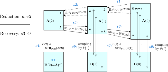
Figure 2: Illustration of Algorithm 1 by using $L=2$. There are mainly two stages with 9 steps. On the reduction stage, we obtain shorter $\mathbf{A}(1)$ and $\mathbf{A}(2)$ by iteratively doing $(R,r)$-projection. On the next recovery stage, we approximate the leverage scores of $\mathbf{A}(1)$ by the ones computed from $\mathbf{A}(2)$ and $\mathbf{B}(2)$. Then $\mathbf{B}(1)$ is sampled based on this approximated scores, which will be used to further obtain the approximated leverage scores of $A(0)$. The final step which samples $\mathbf{B}(0)$ once again is not shown here.

Sampling probabilities for $\mathbf{A}(l-1)$ are obtained by computing the stretch of $\mathbf{A}(l)$ w.r.t. $\mathbf{B}(l)$. We first show these values, $\tilde{{\tau}}(l-1)$, are with high probability upper bounds for the statistical leverage scores of $\mathbf{A}(l-1)$, $\tau(l-1)$.

Lemma 4.13

Assume $\mathbf{A}(l)$ and $\mathbf{B}(l)$ satisfy the following condition

$$\frac{1}{2}\mathbf{A}(l)^{T}\mathbf{A}(l)\preceq\mathbf{B}(l)^{T}\mathbf{B}(l)\preceq\frac{3}{2}\mathbf{A}(l)^{T}\mathbf{A}(l)$$

Then for any constant $c$, there is a setting of the constants such that

• $\tilde{\boldsymbol{\tau}}(l-1)\geq\boldsymbol{\tau}(l-1)$

• $\|\tilde{\boldsymbol{\tau}}(l-1)\|_{1}\leq O(dR^{3}\log{d})$

holds with probability at least $1-d^{-c}$.

Proof The given condition implies that $\sqrt{\frac{2}{3}}\mathbf{B}(l)$ satisfies the condition needed for Lemma 4.6 with $\kappa=3$. Let the constants $c^{\prime}=c+\log_{d}2$, then with probability at least $1-d^{-c^{\prime}}$ we have:

$$\tilde{\boldsymbol{\tau}}^{\prime}(l)\geq O(R^{2}\log d)\boldsymbol{\tau}(l)$$

Since $\mathbf{A}(l)$ is a projection of $\mathbf{A}(l-1)$, we can index corresponding blocks in them. Apply Corollary 4.12, then with probability at least $1-d^{-c^{\prime}}$, we have

$$O(R^{2}\log d)\left\|\boldsymbol{\tau}(l)_{(b)}\right\|_{1}\geq\left\|\boldsymbol{\tau}(l-1)_{(b)}\right\|_{1}$$

for all blocks. As each entries of $\tilde{\boldsymbol{\tau}}(l-1)$ in block $b$ is assigned with $\left\|\tilde{\boldsymbol{\tau}}^{\prime}(l)_{(b)}\right\|_{1}$, by the union bound, then for all $i$ in block $b$

$$\tilde{\boldsymbol{\tau}}(l-1)_{i}=\left\|\tilde{\boldsymbol{\tau}}^{\prime}(l)_{(b)}\right\|_{1}\geq\left\|\boldsymbol{\tau}(l-1)_{(b)}\right\|_{1}\geq\boldsymbol{\tau}(l-1)_{i}$$

holds for all blocks $b$ with probability at least $1-2d^{-c^{\prime}}$, which is equal to $1-d^{-c}$ by the definition of $c^{\prime}$.

It remains to upper bound $\left\|\tilde{\boldsymbol{\tau}}(l-1)\right\|_{1}$. Lemma 4.6 Part 2 gives, with probability at least $1-d^{-c}$, $\left\|\tilde{\boldsymbol{\tau}}^{\prime}(l)\right\|_{1}\leq O(dR^{2}\log d)$. As each $\left\|\tilde{\boldsymbol{\tau}}^{\prime}(l)_{(b)}\right\|_{1}$ is assigned to the $R$ entries in $\tilde{\boldsymbol{\tau}}(l-1)_{(b)}$, we get $\left\|\tilde{\boldsymbol{\tau}}(l-1)\right\|_{1}\leq O(dR^{3}\log{d})$ with the same probability. $\blacksquare$

Combining these with the fact that the number of rows decrease by a factor of $O(R)$ per iteration completes the algorithm. Our main result for $\ell_{2}$ row sampling is obtained by setting $R$ to $d^{\theta}$. Applying Lemma 4.13 inductively backwards in $l$ gives the overall bound.

Theorem 4.14

For any constant $c$, there is a setting of constants such that if RowSampleL2, shown in Algorithm 1, is ran with $R=d^{\theta}$, then with probability at least $1-d^{-c}$ it returns $\mathbf{B}$ in $O(\mathrm{nnz}(\mathbf{A})+d^{\omega+4\theta}\epsilon^{-2})$ time such that:

$$(1-\epsilon)\mathbf{A}^{T}\mathbf{A}\preceq\mathbf{B}^{T}\mathbf{B}\preceq(1+\epsilon)\mathbf{A}^{T}\mathbf{A}$$

and $\mathbf{B}$ has ${O}(d\log{d}\epsilon^{-2})$ rows, each being a scaled copy of some row of $\mathbf{A}$,

Proof We first show correctness via. induction backwards on $l$. Define $c^{\prime}=c+1$, we show that $\mathbf{B}(l)$ has $O(dR^{4}\log{d}\epsilon(l)^{-2})$ rows and satisfies

$$(1-\epsilon(l))\mathbf{A}(l)^{T}\mathbf{A}(l)^{T}\preceq\mathbf{B}(l)^{T}\mathbf{B}(l)\preceq(1+\epsilon(l))\mathbf{A}(l)^{T}\mathbf{A}(l)^{T},$$

with probability at least $1-3(L-l)d^{c^{\prime}}$ for each $l$.

As $k=O({c}/{\theta})$ is a constant, one $(R,k)$-projection decreases the number of rows by a factor of $O(R)$. After $L=\log_{R}(n/d)$ projections, we get that $\mathbf{A}(L)$ has $O(d)$ rows. Therefore the base case where $l=L$ follows from $\mathbf{B}(L)=\mathbf{A}(L)$.

For the inductive step, we assume that the inductive hypothesis holds for $l\geq 1$ and try to show it for $l-1$. As $\epsilon(l)$ was set to $1/2$, we have:

$$\frac{1}{2}\mathbf{A}(l)^{T}\mathbf{A}(l)\preceq\mathbf{B}(l)^{T}\mathbf{B}(l)\preceq\frac{3}{2}\mathbf{A}(l)^{T}\mathbf{A}(l)$$

This allows us to invoke Lemma 4.13, which combined with Lemma 4.1 gives that with probability $1-d^{-c^{\prime}}$, the inductive hypothesis also holds for $l-1$.

The final sampling step on $\mathbf{B}(0)$ with $R=2$ guarantees that $\left\|\tilde{\boldsymbol{\tau}}^{\prime}(0)\right\|_{1}\leq O(d)$, which gives a final row count of $O(d\log d/\epsilon^{2})$. The overall failure probability follows from union bounding this with the failure probabilities from the hypothesis and Lemma 4.13.

We now bound the total running time, starting with the projections. Since $k=O(1)$, each $(R,k)$-projection reduces $R$ rows into $O(1)$ rows, so the sparsity patterns are kept, namely $\mathrm{nnz}(\mathbf{A}(l+1))=O(\mathrm{nnz}(\mathbf{A}(l)))$. As $\mathbf{U}_{(b)}$ has $k$ rows for all $b$, then the cost of constructing $\mathbf{A}(l)$ from $\mathbf{A}(l-1)$ is $O(\mathrm{nnz}(\mathbf{A}))$. Note that since $R=d^{\theta}$, $L=\log_{R}(n/d)=\log_{R}(\mathrm{poly}(d))$ is a constant. So we get a total cost of $O(\mathrm{nnz}(\mathbf{A}))$ over all $L$ projections.

Since $\mathbf{B}(l)$ has $O(dR^{3}\log^{2}d\epsilon(l)^{-2})$ rows, Lemma 4.6 gives that each call to ApproxStr takes $O(\mathrm{nnz}(\mathbf{A})+d^{\omega+4\theta}\epsilon^{-2})$ time, where we upper bound $\log^{2}{d}$ by $d^{\theta}$. The cost of the final step on $\mathbf{B}(0)$ can be bounded similarly. $\blacksquare$

5 Algorithm for Preserving $\ell_{p}$-norm

We now turn to the more general problem of finding $\mathbf{B}$ with $\mathrm{poly}(d)$ rows such that:

$$(1-\epsilon)\left\|\mathbf{A}\mathbf{x}\right\|_{p}\leq\left\|\mathbf{B}\mathbf{x}\right\|_{p}\leq(1+\epsilon)\left\|\mathbf{A}\mathbf{x}\right\|_{p}\qquad\forall\mathbf{x}\in\mathbb{R}^{d}$$

We will make repeated use of the following (tight) inequality between $\ell_{2}$ and $\ell_{p}$ norms, which can be obtained by direct applications of power-mean and Hölder’s inequalities.

Fact 5.1

Let $\mathbf{x}$ be any vector in $\mathbb{R}^{d}$, and $p$ and $q$ any two norms where $1\leq p\leq q$, we have:

$$\left\|\mathbf{x}\right\|_{q}\leq\left\|\mathbf{x}\right\|_{p} \leq d^{\frac{1}{q}-\frac{1}{p}}\left\|\mathbf{x}\right\|_{q}$$

We will use this Fact with one of $p$ or $q$ being $2$, in which case it gives:

• If $1\leq p\leq 2$, $\left\|\mathbf{x}\right\|_{2}\leq\left\|\mathbf{x}\right\|_{p}\leq d^{\frac{1}{2}-\frac{1}{p}}\left\|\mathbf{x}\right\|_{2}$

• If $2\leq p$, $d^{\frac{1}{p}-\frac{1}{2}}\left\|\mathbf{x}\right\|_{2}\leq\left\|\mathbf{x}\right\|_{p}\leq\left\|\mathbf{x}\right\|_{2}$

As $\mathbf{A}\mathbf{x}\in\mathbb{R}^{n}$, its $\ell_{2}$ and $\ell_{p}$ norms can differ by a factor of $\mathrm{poly}(n)$. This means the $\ell_{2}$ row sampling algorithm from Section 4 can lead to $\mathrm{poly}(n)$ distortion. Our algorithm in this section can be viewed as a way to reduce this distortion via. a series of iterative steps. Once again, our algorithm is built around a sampling concentration bound. The sampling probabilities are based on the definition of a well-conditioned basis, which is more flexible than $\ell_{2}$ statistical leverage scores.

Definition 5.2

Let $\mathbf{A}$ be an $n\times d$ matrix of rank $r$, $p\in[1,\infty]$ and $q$ be its dual norm such that $\frac{1}{p}+\frac{1}{q}=1$. Then an $n\times r$ matrix $\mathbf{U}$ is an $(\alpha,\beta,p)$-well-conditioned basis for the column space of $\mathbf{A}$ if the columns of $\mathbf{U}$ span the column space of $\mathbf{A}$ and:

1. ${\left|\kern-0.6458pt\left|\kern-0.6458pt\left|\mathbf{U}\right|\kern-0.6458pt\right|\kern-0.6458pt\right|}_{p}\leq\alpha$.

2. For all $\mathbf{x}\in\mathbb{R}^{r}$, $\left\|\mathbf{x}\right\|_{q}\leq\beta\left\|\mathbf{U}\mathbf{x}\right\|_{p}$.

A $\ell_{p}$ analog of the sampling concentration result given in Lemma 4.1 was shown in [DDH⁺09]. It can be viewed a generalization of Lemma 4.1.

Lemma 5.3

(Theorem 6 of [DDH⁺09]) Let $\mathbf{A}$ be a $n\times d$ matrix with rank $r$, $\epsilon\leq 1/7$, and let $p\in[1,\infty)$. Let $\mathbf{U}$ be an $(\alpha,\beta,p)$-well-conditioned basis for $\mathbf{A}$. Then for any sampling probabilities $\mathbf{p}\in\mathbb{R}^{n}$ such that:

$$p_{i} \geq c_{p}(\alpha\beta)^{p}\frac{\left\|\mathbf{U}_{i*}\right\|^{p}_{p}}{{\left|\kern-0.6458pt\left|\kern-0.6458pt\left|\mathbf{U}\right|\kern-0.6458pt\right|\kern-0.6458pt\right|}^{p}_{p}},$$

where $\mathbf{U}_{i*}$ is the $i$-th row of $\mathbf{U}$ and $c_{p}$ is a constant depending only on $p$. Then with probability at least $1-d^{-c}$, $\textsc{Sample}(\mathbf{A},p,\epsilon)$ returns $\mathbf{B}$ satisfying

$$(1-\epsilon)\left\|\mathbf{A}\mathbf{x}\right\|_{p}\leq\left\|\mathbf{B}\mathbf{x}\right\|_{p}\leq(1+\epsilon)\left\|\mathbf{A}\mathbf{x}\right\|_{p}\qquad\forall\mathbf{x}\in\mathbb{R}^{d}$$

We omitted the reductions of probabilities that are more than $1$ since this step is included in our formulation of Sample. Several additional steps are needed to turn this into an algorithmic routine, the first being computing $\mathbf{U}$. A naïve approach for this requires matrix multiplication, and the size of the outcome may be more than $\mathrm{nnz}(\mathbf{A})$. Alternatively, we can find a linear transform used to create it, aka. a matrix $\mathbf{C}$ such that $\mathbf{U}=\mathbf{A}\mathbf{C}$.

The estimation of $\left\|(\mathbf{A}\mathbf{Q})_{i*}\right\|_{p}^{p}$ and sampling can then be done in a way similar to Section 4. When $1\leq p\leq 2$, we can compute $O(1)$ approximations using $p$-stable distributions [Ind06] in a way analogous to Section 4.2.1. of Clarkson et al. [CDMI⁺12]. When $2\leq p$, we will use the $2$-norm as a surrogate at the cost of more rows. As all of our calls to Sample will be using probabilities estimated via. the same matrix, we will the estimation of $p$-norm leverage scores and sampling as a single blackbox.

Lemma 5.4

For any constant $c$, there exist an algorithm $\textsc{EstimateAndSampleP}(\mathbf{A},\mathbf{C},\alpha,\beta,R,\epsilon)$ that given a $\mathbf{A}$, $\mathbf{C}$ such that $\mathbf{A}\mathbf{C}$ is a $(\alpha,\beta,p)$-well-conditioned basis for $\mathbf{A}$, returns a matrix $\mathbf{B}$ with probability at least $1-d^{-c}$ such that:

$$(1-\epsilon)\|\mathbf{A}\mathbf{x}\|_{p}\leq\|\mathbf{B}\mathbf{x}\|_{p}\leq(1+\epsilon)\|\mathbf{A}\mathbf{x}\|_{p}$$

in $O(\mathrm{nnz}(\mathbf{A})\log_{R}(d)+Rd^{\omega}\log{d})$ time and the number of rows in $\mathbf{B}$ can be bounded by:

$$\begin{cases}O((\alpha\beta R)^{p}d\log(d)\epsilon^{-2})&\textrm{if }1\leq p\leq 2\\ O((\alpha\beta R)^{p}d^{\frac{p}{2}}\log(d)\epsilon^{-2})&\textrm{if }2\leq p\end{cases}$$

5.1 Sampling Using $\ell_{2}$-leverage scores

Our starting point is the observation that a good basis for $\ell_{2}$, specifically a nearly orthonormal basis of $\mathbf{A}$ still allows us to reduce number of rows substantially under $\ell_{p}$.

Lemma 5.5

If $\mathbf{C}\in\mathbb{R}^{d\times r}$ satisfies $\frac{1}{2}(\mathbf{A}^{T}\mathbf{A})^{{\dagger}}\preceq\mathbf{C}\mathbf{C}^{T}\preceq\frac{3}{2}(\mathbf{A}^{T}\mathbf{A})^{{\dagger}}$ then $\mathbf{U}=\mathbf{A}\mathbf{C}$ is a $(\alpha,\beta,p)$-well-conditioned basis for $\mathbf{A}$ where $\alpha\beta\leq O(n^{|\frac{1}{2}-\frac{1}{p}|}d^{|\frac{1}{2}-\frac{1}{p}|+\frac{1}{2}})$.

Proof We start by show that $\mathbf{U}^{T}\mathbf{U}$ is close to the identity matrix as an operator. Also, since $\mathbf{C}^{T}\mathbf{C}$ is a full rank matrix and $\mathbf{C}^{T}(\mathbf{C}\mathbf{C}^{T})^{{\dagger}}\mathbf{C}$ is a projection operator onto the column space of $\mathbf{C}$, we have $\mathbf{C}^{T}(\mathbf{C}\mathbf{C}^{T})^{{\dagger}}\mathbf{C}=\mathbf{I}.$ Taking pseudoinverses of the given condition on $\mathbf{C}$ gives:

$$\frac{2}{3}(\mathbf{C}\mathbf{C}^{T})^{{\dagger}} \preceq\mathbf{A}^{T}\mathbf{A}\preceq 2(\mathbf{C}\mathbf{C}^{T})^{{\dagger}}$$

Substituting it into $\mathbf{U}=\mathbf{A}\mathbf{C}$ then gives:

$$\mathbf{U}^{T}\mathbf{U}=\mathbf{C}^{T}\mathbf{A}^{T}\mathbf{A}\mathbf{C}\preceq 2\mathbf{C}^{T}(\mathbf{C}\mathbf{C}^{T})^{{\dagger}}\mathbf{C}=2\mathbf{I}$$

and

$$\frac{2}{3}\mathbf{I}\preceq\frac{2}{3}\mathbf{C}^{T}(\mathbf{C}\mathbf{C}^{T})^{{\dagger}}\mathbf{C}\preceq\mathbf{U}^{T}\mathbf{U}$$

This allows us to infer that ${\left|\kern-0.6458pt\left|\kern-0.6458pt\left|\mathbf{U}\right|\kern-0.6458pt\right|\kern-0.6458pt\right|}_{2}\leq\sqrt{2d}$, and for any vector $\mathbf{x}$, $\left\|\mathbf{x}\right\|_{2}\leq\sqrt{2}\left\|\mathbf{U}\mathbf{x}\right\|_{2}$.

Next we find values of $\alpha$ and $\beta$ that meet the requirements of a well-conditioned basis given in Definition 5.2. Let $q$ be the dual norm for $p$ which satisfies $\frac{1}{p}+\frac{1}{q}=1$.

First consider the case where $1\leq p\leq 2$. We can view all entries of the matrix $\mathbf{U}$ as a vector of length $nr\leq nd$ vector. Apply Fact 5.1 gives:

$${\left|\kern-0.6458pt\left|\kern-0.6458pt\left|\mathbf{U}\right|\kern-0.6458pt\right|\kern-0.6458pt\right|}_{p} \leq(nd)^{\frac{1}{p}-\frac{1}{2}}{\left|\kern-0.6458pt\left|\kern-0.6458pt\left|\mathbf{U}\right|\kern-0.6458pt\right|\kern-0.6458pt\right|}_{2}$$

Which gives ${\left|\kern-0.6458pt\left|\kern-0.6458pt\left|\mathbf{U}\right|\kern-0.6458pt\right|\kern-0.6458pt\right|}_{2}\leq\sqrt{2}d^{\frac{1}{2}}$ and therefore $\alpha=\sqrt{2}(nd)^{\frac{1}{p}-\frac{1}{2}}d^{\frac{1}{2}}$. For the second part, given any vector $\mathbf{x}$, we have

$$\left\|\mathbf{x}\right\|_{q} \leq\left\|\mathbf{x}\right\|_{2} \mathbf{x} q\leq 2$$ (by Fact 5.1 on since )

$$\leq\sqrt{2}\left\|\mathbf{U}\mathbf{x}\right\|_{2}$$

$$\leq\sqrt{2}\left\|\mathbf{U}\mathbf{x}\right\|_{p} \mathbf{U}\mathbf{x} 1\leq p\leq 2$$ (by Fact 5.1 on since )

which means $\beta=\sqrt{2}$ suffices.

Now we consider the case where $p\geq 2$ similarly.

$${\left|\kern-0.6458pt\left|\kern-0.6458pt\left|\mathbf{U}\right|\kern-0.6458pt\right|\kern-0.6458pt\right|}_{p}\leq{\left|\kern-0.6458pt\left|\kern-0.6458pt\left|\mathbf{U}\right|\kern-0.6458pt\right|\kern-0.6458pt\right|}_{2}\leq\sqrt{2}d^{1/2}$$

and:

$$\left\|\mathbf{x}\right\|_{q} \leq d^{\frac{1}{q}-\frac{1}{2}}\left\|\mathbf{x}\right\|_{2} \mathbf{x} q\leq 2$$ (by Fact 5.1 on since )

$$=d^{\frac{1}{2}-\frac{1}{p}}\left\|\mathbf{x}\right\|_{2} \frac{1}{q}=1-\frac{1}{p}$$ (since )

$$\leq\sqrt{2}d^{\frac{1}{2}-\frac{1}{p}}\left\|\mathbf{U}\mathbf{x}\right\|_{2}$$

$$\leq\sqrt{2}d^{\frac{1}{q}-\frac{1}{2}}n^{\frac{1}{2}-\frac{1}{p}}\left\|\mathbf{U}\mathbf{x}\right\|_{p} \mathbf{U}\mathbf{x} 2\leq p$$ (by Fact 5.1 on with )

$$=\sqrt{2}(nd)^{\frac{1}{2}-\frac{1}{p}}\left\|\mathbf{U}\mathbf{x}\right\|_{p}\$$

Combining the bounds from these two cases on $p$ gives that $U$ is a $(\alpha,\beta,p)-$well-conditioned basis, where

$$\alpha=\begin{cases}\sqrt{2}d^{\frac{1}{2}}&\textrm{for }p\geq 2\\ \sqrt{2}(nd)^{\frac{1}{p}-\frac{1}{2}}d^{\frac{1}{2}}&\textrm{otherwise }\end{cases}\quad\textrm{and}\quad\beta=\begin{cases}\sqrt{2}(nd)^{\frac{1}{2}-\frac{1}{p}}&\textrm{for }p\geq 2\\ \sqrt{2}&\textrm{otherwise}\end{cases}$$

It can be checked that in both cases the stated bound on $\alpha\beta$ holds. $\blacksquare$

One way to generate such a nearly-orthonormal basis is by the $L_{2}$ approximation that we computed in Section 4. This leads to a fast algorithm, but the dependency on $n$ in this bound precludes a single application of sampling using the values given because each time we transfer $n$ rows into $O(p|\frac{1}{2}-\frac{1}{p}|)$ rows. However, note that when $p<4$, $p|\frac{1}{2}-\frac{1}{p}|=|1-\frac{p}{2}|<1$. This means it can be used as a reduction step in an iterative algorithm where the number of rows will decrease geometrically. Therefore, we can use this process as a reduction routine. For inductive purposes, we will also state the routine to compute the basis via. an approximation of $\mathbf{A}$, $\tilde{\mathbf{A}}$. Pseudocode of our reduction algorithm is given in Algorithm 2.

$\textsc{ReduceP}(\mathbf{A},\tilde{\mathbf{A}},\epsilon)$

Input: $n\times d$ matrix $\mathbf{A}$ and its approximated matrix $\tilde{\mathbf{A}}$, $p$-norm and error parameter $\epsilon$

Output: Matrix $\mathbf{B}$

1:  $\mathbf{A}\textrm{\tiny$\downarrow$}\leftarrow\textsc{RowCombine}(\tilde{\mathbf{A}},p,1/3,d^{-c-1})$

2:  Perform SVD on $\mathbf{A}\textrm{\tiny$\downarrow$}^{T}\mathbf{A}\textrm{\tiny$\downarrow$}$ and then construct $\mathbf{C}$ by dropping the zero singular values and corresponding singular vectors such that $\mathbf{C}^{T}\mathbf{C}=(\mathbf{A}\textrm{\tiny$\downarrow$}^{T}\mathbf{A}\textrm{\tiny$\downarrow$})^{{\dagger}}$

3:  if $1\leq p\leq 2$ then

4:     $\alpha\leftarrow\sqrt{2}(nd)^{\frac{1}{p}-\frac{1}{2}}d^{\frac{1}{2}}$, $\beta\leftarrow\sqrt{2}$

5:  else

6:     $\alpha\leftarrow\sqrt{2}d^{\frac{1}{2}}$, $\beta\leftarrow\sqrt{2}(nd)^{\frac{1}{2}-\frac{1}{p}}$

7:  end if

8:  $\mathbf{B}\leftarrow\textsc{EstimeAndSampleP}(\mathbf{A},\mathbf{C},2\alpha,2\beta,p,d^{\frac{\theta}{2p}},\epsilon)$

9:  return  $\mathbf{B}$

Algorithm 2 Reduction Step for Preserving $\ell_{p}$ Norm

Lemma 5.6

For any constant $c$, there exist a setting of constants in ReduceP such that if $\mathbf{A}$ and $\tilde{\mathbf{A}}$ satisfy

$$\frac{1}{2}\left\|\mathbf{A}\mathbf{x}\right\|_{p}\leq\left\|\tilde{\mathbf{A}}\mathbf{x}\right\|_{p}\leq\frac{3}{2}\left\|\mathbf{A}\mathbf{x}\right\|_{p}\qquad\forall\mathbf{x}\in\mathbb{R}^{d}$$

and $\tilde{\mathbf{A}}$ has $\tilde{n}$ rows, then $\textsc{ReduceP}(\mathbf{A},\tilde{\mathbf{A}},\epsilon)$ returns in $O(\mathrm{nnz}(\mathbf{A})\log{d+\theta}+d^{\omega+\theta}\log{d})$ time a matrix $\mathbf{B}$ such that with probability at least $1-d^{-c}$:

$$(1-\epsilon)\left\|\mathbf{A}\mathbf{x}\right\|_{p}\leq\left\|\mathbf{B}\mathbf{x}\right\|_{p}\leq(1+\epsilon)\left\|\mathbf{A}\mathbf{x}\right\|_{p}\qquad\forall\mathbf{x}\in\mathbb{R}^{d}$$

And the number of rows in $\mathbf{B}$ can be bounded by:

$$\begin{cases}O(n^{1-\frac{p}{2}}d^{2+\theta}\epsilon^{-2})&\text{if }1\leq p\leq 2\\ O(n^{\frac{p}{2}-1}d^{\frac{3}{2}p-1+\theta}\epsilon^{-2})&\text{if }2\leq p\end{cases}$$

The proof will be in two steps: we first show that $\tilde{\mathbf{A}}\mathbf{C}$ is a well-conditioned basis for $\tilde{\mathbf{A}}$, and use the following Lemma to show that this implies that $\mathbf{A}\mathbf{C}$ is a well-conditioned basis for $\mathbf{A}$.

Lemma 5.7

If $\mathbf{A}$ and $\tilde{\mathbf{A}}$ are such that for all $\mathbf{x}\in\mathbb{R}^{d}$, $\frac{1}{2}\left\|\mathbf{A}\mathbf{x}\right\|_{p}\leq\|\tilde{\mathbf{A}}\mathbf{x}\|_{p}\leq\frac{3}{2}\left\|\mathbf{A}\mathbf{x}\right\|_{p}$, and $\mathbf{C}$ is such that $\tilde{\mathbf{U}}=\tilde{\mathbf{A}}\mathbf{C}$ is an $(\alpha,\beta,p)$-well-conditioned basis for $\mathbf{A}$, then $\mathbf{A}\mathbf{C}$ is also an $(2\alpha,2\beta,p)$-well-conditioned basis for $\mathbf{A}$.

Proof It suffices to verify both conditions of Definition 5.2 holds for $\mathbf{U}=\mathbf{A}\mathbf{C}$. For ${\left|\kern-0.6458pt\left|\kern-0.6458pt\left|\mathbf{U}\right|\kern-0.6458pt\right|\kern-0.6458pt\right|}_{p}$, we can treat its $p$^th power as a summation over the columns of $\mathbf{U}$ and get:

$${\left|\kern-0.6458pt\left|\kern-0.6458pt\left|\mathbf{U}\right|\kern-0.6458pt\right|\kern-0.6458pt\right|}_{p}^{p} =\sum_{j=1}^{d}\left\|\mathbf{U}_{*j}\right\|_{p}^{p}=\sum_{j=1}^{d}\left\|\mathbf{A}\mathbf{C}_{*j}\right\|_{p}^{p}$$

$$\leq\sum_{j=1}^{d}{2}^{p}\left\|\tilde{\mathbf{A}}\mathbf{C}_{*j}\right\|_{p}^{p} \frac{1}{2}\left\|\mathbf{A}\mathbf{x}\right\|_{p}\leq\|\tilde{\mathbf{A}}\mathbf{x}\|_{p}$$ (by assumption )

$$={2}^{p}{\left|\kern-0.6458pt\left|\kern-0.6458pt\left|\tilde{\mathbf{U}}\right|\kern-0.6458pt\right|\kern-0.6458pt\right|}^{p}_{p}=2^{p}\alpha^{p}$$

The other condition can be obtained by direct substitution. By the condition given, we have that for all $\mathbf{z}\in\mathbb{R}^{d}$:

$$\left\|\mathbf{z}\right\|_{q} \leq\beta\left\|\tilde{\mathbf{U}}\mathbf{z}\right\|_{p}=\beta\left\|\tilde{\mathbf{A}}\mathbf{C}\mathbf{z}\right\|_{p}$$

Applying the fact that $\left\|\mathbf{A}\mathbf{x}\right\|_{p}\leq 2\|{\tilde{\mathbf{A}}\mathbf{x}}\|_{p}$ to the vector $\mathbf{C}\mathbf{z}$ gives:

$$\left\|\mathbf{z}\right\|_{q} \leq\beta(2\left\|\mathbf{A}\mathbf{C}\mathbf{z}\right\|_{p})=2\beta\left\|\mathbf{U}\mathbf{z}\right\|_{p}$$

$\blacksquare$

Proof of Lemma 5.6:  By the guarantees of RowCombineL2 given in Theorem 4.14, we can set its constants so that with probability at least $1-d^{-c^{\prime}}$ we have:

$$\frac{1}{2}\tilde{\mathbf{A}}^{T}\tilde{\mathbf{A}}\preceq\mathbf{A}\textrm{\tiny$\downarrow$}^{T}\mathbf{A}\textrm{\tiny$\downarrow$}\preceq\frac{3}{2}\tilde{\mathbf{A}}^{T}\tilde{\mathbf{A}}.$$

As $\mathbf{C}^{T}\mathbf{C}=(\mathbf{A}\textrm{\tiny$\downarrow$}^{T}\mathbf{A}\textrm{\tiny$\downarrow$})^{\dagger}$, then the condition of Lemma 5.5 is satisfied, so $\tilde{\mathbf{A}}\mathbf{C}$ is a well-conditioned basis of $\tilde{\mathbf{A}}$. Furthermore, by Lemma 5.7, $\mathbf{A}\mathbf{C}$ is also a well-conditioned basis of $\mathbf{A}$. The guarantees for $\mathbf{B}$ then follows from Lemma 5.4. The probability can be obtained by a simply union bound with $c^{\prime}=c+\log 2$. $\blacksquare$

Iterating this reduction routine with $\tilde{\mathbf{A}}=\mathbf{A}$ gives a way to reduce the row count from $n$ to $\mathrm{poly}(d)$ in $O(\log\log(n/d))$ iterations when $p<4$. Two issues remain: the approximation errors will accumulate across the iterations, and it’s rather difficult (although possible if additional factors of $d$ are lost) to bound the reductions of non-zeros since different rows may have different numbers of them. We will address these two issues systematically before giving our complete algorithm.

The only situation where a large decrease in the number of rows does not significantly decrease the overall number of non-zeros is when most of the non-zeros are in a few rows. A simple way to get around this is to ‘bucket’ the rows of $\mathbf{A}$ by their number of non-zeros, and compute $\mathrm{poly}(d)$ sized samples of each bucket separately. This incurs an extra factor of $\log{d}$ in the final number of rows, but ensures a geometric reduction in problem sizes as we iterate.

The error buildup can in turn be addressed by sampling on the rows of the initial $\mathbf{A}$ using the latest approximation for it $\tilde{\mathbf{A}}$. However, since the algorithm can take up to $O(\log{d})$ iterations, we need to perform this on a reduced version of $\mathbf{A}$ instead to obtain a $O(\mathrm{nnz}(\mathbf{A}))$ running time. Pseudocode of our algorithm for a single partition where the number of non-zeros in each row are within a constant factor of each other is given in Algorithm 3.

Algorithm 3 Algorithm for Producing Row Sample of Size $\mathrm{poly}(d)$ that Preserves $\ell_{p}$-norm

$\textsc{RowSampleP}(\mathbf{A},p,\epsilon,\delta)$

Input: $n\times d$ matrix $\mathbf{A}$, $p$, error parameter $\epsilon$, failure probability $\delta=d^{-c}$

Output: Matrix $\mathbf{B}$

1:  if $1\leq p\leq 2$ then

2:     $n^{*}\leftarrow O(d^{\frac{4}{p}+\theta}\log^{\frac{2}{p}}d)$

3:  else

4:     $n^{*}\leftarrow O(d^{\frac{3}{2}p-1+\theta}\log^{\frac{3p-2}{4-p}}{d})$

5:  end if

6:  if $\mathbf{A}$ has $n^{*}$ or fewer rows then

7:     return  $\mathbf{A}$

8:  end if

9:  $\tilde{\mathbf{A}}_{0},\tilde{\mathbf{A}}\leftarrow\textsc{ReduceP}(\mathbf{A},\mathbf{A},1/5)$

10:  while $\tilde{\mathbf{A}}$ has more than $\bar{n}$ rows do

11:     $\tilde{\mathbf{A}}\leftarrow\textsc{ReduceP}(\tilde{\mathbf{A}}_{0},\tilde{\mathbf{A}},1/5)$

12:  end while

13:  $\mathbf{B}\leftarrow\textsc{ReduceP}(\mathbf{A},\tilde{\mathbf{A}},\epsilon/2)$

14:  return  $\mathbf{B}$

Lemma 5.8

For any $c$, there is a setting of constants in RowSample such that given a matrix $\mathbf{A}$ where each row has between $[s,2s]$ nonzeros and $p<4$. $\textsc{RowSampleP}(\mathbf{A},p,\epsilon)$ with probability $1-d^{-c}$ returns in $O(\mathrm{nnz}(\mathbf{A})+d^{\omega}\log{d})$ time a matrix $\mathbf{B}$ such that:

$$(1-\epsilon)\left\|\mathbf{A}\mathbf{x}\right\|_{p}\leq\left\|\mathbf{B}\mathbf{x}\right\|_{p}\leq(1+\epsilon)\left\|\mathbf{A}\mathbf{x}\right\|_{p}$$

And the number of rows in $\mathbf{B}$ can be bounded by

$$\begin{cases}O(d^{\frac{4}{p}+\theta}\epsilon^{-2})&\text{if }1\leq p\leq 2\\ O(d^{\frac{3}{2}p-1+\theta}\epsilon^{-2})&\text{if }2\leq p\leq 4\end{cases}$$

Proof For correctness, we can show by induction that as long as all calls to ReduceP succeeds, $\left|\left\|\tilde{\mathbf{A}}_{0}\mathbf{x}\right\|_{p}-\left\|\tilde{\mathbf{A}}\mathbf{x}\right\|_{p}\right|\leq 1/5\left\|\tilde{\mathbf{A}}_{0}\mathbf{x}\right\|_{p}$ for all $\mathbf{x}\in\mathbb{R}^{d}$. This can be combined with the guarantee between $\mathbf{A}$ and $\tilde{\mathbf{A}}$ to give: $\left|\left\|\mathbf{A}\mathbf{x}\right\|_{p}-\left\|\tilde{\mathbf{A}}\mathbf{x}\right\|_{p}\right|\leq 1/2\left\|\mathbf{A}\mathbf{x}\right\|_{p}$ for all $\mathbf{x}\in\mathbb{R}^{d}$, which allows us to obtain the bound on $\mathbf{B}$. The analysis below shows that there can be at most $O(\log{d})$ calls to ReduceP, so calling each with success probability at least $1-d^{-c-2}$ gives an overall success probability of at least $1-d^{-c-1}$.

To bound the runtime, we first show that if $\mathbf{B}$ has $n_{b}$ rows, then in the next iteration the number of rows in $\mathbf{B}$ can be bounded by $(n_{b}/n*)^{c_{p}}n*$ where $c_{p}<1$ is a constant based on $p$. When $1\leq p\leq 2$, Lemma 5.6 gives that there exist some constant $c_{0}$ such that the new row count can be bounded by:

$$c_{0}n_{b}^{1-\frac{p}{2}}d^{2+\theta}\log(d)=(n_{b}c_{0}^{-\frac{2}{p}}d^{-\frac{4}{p}-\frac{2\theta}{p}}\log^{-\frac{2}{p}}{d})^{1-\frac{p}{2}}c_{0}^{\frac{2}{p}}d^{\frac{4}{p}+\frac{2\theta}{p}}\log^{\frac{2}{p}}{d}$$

So $n^{*}=c_{0}^{\frac{2}{p}}d^{\frac{4}{p}+O(\theta)}\log^{\frac{2}{p}}{d}$ and $c_{p}=1-\frac{p}{2}$ suffices. Similarly for the case where $2\leq p$, it can be checked that

$$n^{*}=c_{0}^{\frac{2}{4-p}}d^{\frac{3p-2}{4-p}+O(\theta)}\log^{\frac{2}{4-p}}{d}$$

Gives that the new row count can be bounded by $(n_{b}/n^{*})^{c_{p}}n^{*}$ where $c_{p}=\frac{p}{2}-1$. As we can set $\theta$ to any arbitrary constant, the constant in front of its exponent can also be removed.

Therefore in $O(\log_{c_{p}^{-1}}(\log(n/n^{*}))=O(\log\log{n})$ iterations the number of rows in $\mathbf{B}$ decreases below $2n^{*}$. Also, the number of rows in $\tilde{\mathbf{A}}$ is at most $(n/n^{*})^{c_{p}}n^{*}=n(n/n^{*})^{c_{p}-1}$. This means the total cost to obtain the final $\mathbf{B}$ can be bounded by $O(\mathrm{nnz}(\mathbf{A})+(\mathrm{nnz}(\mathbf{A})(n/n^{*})^{c_{p}-1}+d^{\omega+\theta}\log(n/n^{*})))$ Since $\log{t}\leq O(t^{1-c_{p}})$, the first two terms can be bounded by $O(\mathrm{nnz}(\mathbf{A}))$. The overall runtime bound then follows by applying Lemma 5.6 to the final call of ReduceP.

$\blacksquare$

5.2 Fewer Rows by Iterating Again

A closer look at the proof of Lemma 5.8 shows that a significant increase in the number of rows comes from dividing by the $1-|1-\frac{p}{2}|$ term in the exponent of $n$. As a result, the row count can be further reduced if the leverage scores are computed via. a $p^{\prime}$-norm approximation where $q$ is between $2$ and $p$. For simplicity we only show this improvement for the case where $1\leq p\leq p^{\prime}\leq 2$.

We will start by proving a generalization of Lemma 5.5.

Lemma 5.9

If $\mathbf{A}$ has rank $r$, $1\leq p\leq p^{\prime}\leq 2$, and $\tilde{\mathbf{A}}$ is a matrix with $\tilde{n}$ rows such that for all vectors $\mathbf{x}$ we have $\frac{1}{2}\left\|\mathbf{A}\mathbf{x}\right\|_{q}\leq\left\|\tilde{\mathbf{A}}\mathbf{x}\right\|_{q}\leq\frac{3}{2}\left\|\mathbf{A}\mathbf{x}\right\|_{q}$, and $\mathbf{C}$ is a $d\times r$ matrix such that $\frac{1}{2}(\tilde{\mathbf{A}}^{T}\tilde{\mathbf{A}})^{{\dagger}}\preceq\mathbf{C}\mathbf{C}^{T}\preceq\frac{3}{2}(\tilde{\mathbf{A}}^{T}\tilde{\mathbf{A}})^{{\dagger}}$, then $\mathbf{U}=\mathbf{A}\mathbf{C}$ is a $(\alpha,\beta,p)$-well-conditioned basis for $\mathbf{A}$ where $\alpha\beta\leq O(n^{\frac{1}{p}-\frac{1}{p^{\prime}}}\tilde{n}^{\frac{1}{p^{\prime}}-\frac{1}{2}}d^{\frac{1}{p}})$.

Proof Let $\tilde{\mathbf{U}}=\tilde{\mathbf{A}}\mathbf{C}$. Similar to the proof of Lemma 5.5, we have ${\left|\kern-0.6458pt\left|\kern-0.6458pt\left|\tilde{\mathbf{U}}\right|\kern-0.6458pt\right|\kern-0.6458pt\right|}_{2}\leq\sqrt{2d}$, and $\left\|\mathbf{x}\right\|_{2}\leq\sqrt{2}\left\|\tilde{\mathbf{U}}\mathbf{x}\right\|_{2}$ for any vector $\mathbf{x}$. Once again, let $q$ be the dual norm for $p$ such that $\frac{1}{p}+\frac{1}{q}=1$.

We have:

$${\left|\kern-0.6458pt\left|\kern-0.6458pt\left|\mathbf{A}\mathbf{C}\right|\kern-0.6458pt\right|\kern-0.6458pt\right|}_{p} \leq(nd)^{\frac{1}{p}-\frac{1}{p^{\prime}}}{\left|\kern-0.6458pt\left|\kern-0.6458pt\left|\mathbf{A}\mathbf{C}\right|\kern-0.6458pt\right|\kern-0.6458pt\right|}_{p^{\prime}}$$

$$\leq(nd)^{\frac{1}{p}-\frac{1}{p^{\prime}}}\left(3/2{\left|\kern-0.6458pt\left|\kern-0.6458pt\left|\tilde{\mathbf{A}}\mathbf{C}\right|\kern-0.6458pt\right|\kern-0.6458pt\right|}_{p^{\prime}}\right)$$

$$\leq 3/2(nd)^{\frac{1}{p}-\frac{1}{p^{\prime}}}(\tilde{n}d)^{\frac{1}{p^{\prime}}-\frac{1}{2}}{\left|\kern-0.6458pt\left|\kern-0.6458pt\left|\tilde{\mathbf{A}}\mathbf{C}\right|\kern-0.6458pt\right|\kern-0.6458pt\right|}_{2}$$

Which gives $\alpha=O(n^{\frac{1}{p}-\frac{1}{p^{\prime}}}\tilde{n}^{\frac{1}{p^{\prime}}-\frac{1}{2}}d^{\frac{1}{p}})$. Also,

$$\left\|\mathbf{x}\right\|_{q}\leq\left\|\mathbf{x}\right\|_{2}\leq 2\left\|\tilde{\mathbf{A}}\mathbf{C}\mathbf{x}\right\|_{2}\leq 3\left\|\mathbf{A}\mathbf{C}\mathbf{x}\right\|_{p^{\prime}}\leq 3\left\|\mathbf{A}\mathbf{C}\mathbf{x}\right\|_{p}$$

Which gives $\beta=O(1)$.

$\blacksquare$

This allows us to compute leverage scores via. a $\ell_{p^{\prime}}$-norm approximation. By Lemma 5.8, such a matrix has $\tilde{n}=O(d^{\frac{4}{p^{\prime}}}\log^{\frac{2}{p^{\prime}}}{d})$ rows. By Lemma 5.4, the resulting number of rows can be bounded by:

$$O\left(\left(n^{\frac{1}{p}-\frac{1}{p^{\prime}}}\tilde{n}^{\frac{1}{p^{\prime}}-\frac{1}{2}}d^{\frac{1}{p}}R\right)^{p}d\log{d}\right)=O\left(n^{1-\frac{p}{p^{\prime}}}\left(d^{\frac{4}{p^{\prime}}}\log^{\frac{2}{p^{\prime}}}{d}\right)^{\frac{p}{p^{\prime}}-\frac{p}{2}}R^{p}d^{2}\log^{\frac{2p}{p^{\prime}}+1}{d}\right)$$

This leads to a result analogous to Lemma 5.6. Solving for the fixed point of this process allows us to prove Theorem 2.2.

Proof of Theorem 2.2:  Similar to the proof of Lemma 5.8, in each iteration we reduce the number of rows from $n$ to $O\left(n^{1-\frac{p}{p^{\prime}}}\left(d^{\frac{4}{p^{\prime}}}\log^{\frac{2}{p^{\prime}}}{d}\right)^{\frac{p}{p^{\prime}}-\frac{p}{2}}R^{p}d^{2}\log^{\frac{2p}{p^{\prime}}+1}{d}\right)$. Ignoring terms in $R$ and $\log{d}$, we have that the number of rows converges doubly exponentially towards:

$$\left(\left(d^{\frac{4}{p^{\prime}}}\right)^{\frac{p}{p^{\prime}}-\frac{p}{2}}d^{2}\right)^{\frac{p^{\prime}}{p}} =d^{\frac{4}{p^{\prime}}-2+2\frac{p^{\prime}}{p}}=d^{\frac{4}{p^{\prime}}+2p^{\prime}-2}$$

This is minimized when $p^{\prime}=\sqrt{2}$, giving $\frac{4}{p^{\prime}}+2p^{\prime}-2=4\sqrt{2}-2$. As we can set $R=d^{O(\theta)}$, the number of rows in $\mathbf{B}$ can be bounded by $O(d^{4\sqrt{2}-2+\theta})$ for any constant $\theta$. $\blacksquare$

This method can be used to reduce the number of rows for all values of $1\leq p\leq 2$. A calculation similar to the above proof leads to a row count of $O(d^{\sqrt{\frac{8}{p}}-2})$. However, using three or more steps does not lead to a significantly better bound since we can only obtain samples with about $d$ rows when $p=2$. For $p\geq 4$, multiple steps of this approach also allows us to compute $\mathrm{poly}(d)$ sized samples for any value of $p$. We omit this extension as it leads to a significantly higher row count.

Appendix A Properties and Estimation of Stretch and Leverage Scores

A.1 Properties of Generalized Stretch

We now give proofs for estimating leverage scores and row sampling that we stated in Sections 4 and 5.

Proof of Fact 4.2:

$$\sum_{i=1}^{n}\mathrm{STR}_{\mathbf{A}}(\mathbf{a}_{i}) =\sum_{i=1}^{n}\mathbf{a}_{i}(\mathbf{A}^{T}\mathbf{A})^{{\dagger}}\mathbf{a}_{i}^{T}$$

$$=\sum_{i=1}^{n}\textrm{tr}\left[(\mathbf{A}^{T}\mathbf{A})^{{\dagger}}\mathbf{a}_{i}^{T}\mathbf{a}_{i}\right]$$

$$=\textrm{tr}\left[(\mathbf{A}^{T}\mathbf{A})^{{\dagger}}\sum_{i=1}^{n}\mathbf{a}_{i}^{T}\mathbf{a}_{i}\right]$$

$$=\textrm{tr}\left[(\mathbf{A}^{T}\mathbf{A})^{{\dagger}}\mathbf{A}^{T}\mathbf{A}\right]=r$$ (1.4)

$\blacksquare$

Proof of Fact 4.4:  Note that both stretch and the Frobenius norm acts on the rows independently. Therefore it suffices to prove this when $\mathbf{A}^{\prime}$ has a single row, aka. $\mathbf{A}^{\prime}=\mathbf{a}$. In this case the cyclic property of trace gives:

$$\mathrm{STR}_{\mathbf{A}}(\mathbf{a}) =\mathbf{a}(\mathbf{A}^{T}\mathbf{A})^{{\dagger}}\mathbf{a}^{T}$$

$$=\mathbf{a}(\mathbf{A}^{T}\mathbf{A})^{{\dagger}1/2}(\mathbf{A}^{T}\mathbf{A})^{{\dagger}1/2}\mathbf{a}^{T}$$

$$=\left\|\mathbf{A}^{{\dagger}1/2}\mathbf{a}^{T}\right\|_{2}^{2}$$ (1.5)

$\blacksquare$

Proof of Lemma 4.3:  The condition given implies that the null spaces of $\mathbf{B}_{1}^{T}\mathbf{B}_{1}$ and $\mathbf{B}_{2}^{T}\mathbf{B}_{2}$ are identical, giving:

$$(\mathbf{B}_{1}^{T}\mathbf{B}_{1})^{{\dagger}}\preceq(\mathbf{B}_{2}^{T}\mathbf{B}_{2})^{{\dagger}}\preceq\kappa(\mathbf{B}_{1}^{T}\mathbf{B}_{1})^{{\dagger}}$$ (1.6)

Applying this to the vector $\mathbf{x}$ gives:

$$\mathbf{x}(\mathbf{B}_{1}^{T}\mathbf{B}_{1})^{{\dagger}}\mathbf{x}^{T}\leq \mathbf{x}(\mathbf{B}_{2}^{T}\mathbf{B}_{2})^{{\dagger}}\mathbf{x}^{T}\leq\kappa\mathbf{x}(\mathbf{B}_{1}^{T}\mathbf{B}_{1})^{{\dagger}}\mathbf{x}^{T}$$ (1.7)

$\blacksquare$

A.2 Estimation of Generalized Stretch

Based on this fact, we can estimate these scores using randomized projections in a way that’s by now standard [SS08, DMIMW12]. Pseudocode of our estimation algorithm is shown in Algorithm 4, while the error analysis is nearly identical to the ones given in Section 4 of [SS08] and Section 3.2. of [DMIMW12].

$\textsc{ApproxStr}(\mathbf{A},\mathbf{B},\kappa,R)$

Input: A $n\times d$ matrix $\mathbf{A}$, approximation $m\times d$ matrix $\mathbf{B}$ such that $\frac{1}{\kappa}\mathbf{A}^{T}\mathbf{A}\preceq\mathbf{B}^{T}\mathbf{B}\preceq\mathbf{A}^{T}\mathbf{A}$, parameter $R\geq e^{2}$ indicating allowed estimation error.

Output: Upper bounds for stretches of rows of $\mathbf{A}$ measured $\tilde{{\tau}}_{1}\ldots\tilde{{\tau}}_{n}$.

  Compute $\mathbf{C}=(\mathbf{B}^{T}\mathbf{B})^{{\dagger}\frac{1}{2}}$

  Let $k=O(\log_{R}(1/\delta))$

  Let $\mathbf{U}$ be a $k\times d$ matrix with each entry is picked independently from $\mathcal{N}(0,1)$

  Let $\tilde{{\tau}}_{i}=\frac{R}{d}\left\|\mathbf{U}\mathbf{C}\mathbf{a}_{i}^{T}\right\|_{2}^{2}$.

  return  $\tilde{\boldsymbol{\tau}}$

Algorithm 4 Algorithm for Upper Bounding Stretch

We remark that $(\mathbf{B}^{T}\mathbf{B})^{{\dagger}\frac{1}{2}}$ can be replaced by any matrix whose product with its transpose equals to $\mathbf{B}^{T}\mathbf{B}$. nee candidate for this is $\mathbf{B}(\mathbf{B}^{T}\mathbf{B})^{{\dagger}}$, and using it would avoid computing the $1/2$ power of a matrix. However, from a theoretical point of view both of these operations take $O(md^{\omega-1})$ time, and we omit this extra step for simplicity.

Proof of Lemma 4.6:

Since $\mathbf{B}^{T}\mathbf{B}\preceq\mathbf{A}^{T}\mathbf{A}$ by assumption, then $\left(\mathbf{A}^{T}\mathbf{A}\right)^{\dagger}\preceq\left(\mathbf{B}^{T}\mathbf{B}\right)^{\dagger}$. Denote by $\tau^{\prime}_{i}=\mathrm{STR}_{\mathbf{B}}(\mathbf{a}_{i})=\mathbf{a}_{i}\left(\mathbf{B}^{T}\mathbf{B}\right)^{\dagger}\mathbf{a}_{i}^{T}$, note that $\tau_{i}=\mathrm{STR}_{\mathbf{A}}(\mathbf{a}_{i})=\mathbf{a}_{i}\left(\mathbf{A}^{T}\mathbf{A}\right)^{\dagger}\mathbf{a}_{i}^{T}$, we have $\tau^{\prime}_{i}\geq\tau_{i}$. Next we show u $\tilde{\tau}_{i}\geq\tau^{\prime}_{i}$ holds with large probability. By Lemma 4.5 Part 3 we have:

$$\Pr\left[\tilde{\tau}_{i}\leq\tau^{\prime}_{i}\right] =\Pr\left[\frac{1}{k}\left\|\mathbf{U}\mathbf{C}\mathbf{a}_{i}^{T}\right\|_{2}^{2}\leq\frac{1}{R}\left\|\mathbf{C}\mathbf{a}_{i}^{T}\right\|_{2}^{2}\right]$$

$$\leq\exp\left(\frac{k}{2}(1-R^{-1}-\ln{R}))\right)$$

$$\leq\exp\left(-\frac{k}{2}\frac{\ln{R}}{2}\right)$$

$$=R^{-\frac{k}{4}},$$

where the last inequality is due to the assumption that $R\leq e^{2}$. By a suitable choice of constants in $k=O(\log_{R}{nd^{c}})=O(\log_{R}d)$ this can be made the above probability less than $n^{-1}d^{-c}$, taking a union bound over the $n$ rows gives Part 1.

The upper bound on $\|\tilde{\boldsymbol{\tau}}\|_{1}$ can be obtained similarly. From Lemma 4.3, we have $\tau^{\prime}_{i}\leq\kappa\tau_{i}$ holds for all $i$. Then using Part 2 of Lemma 4.5:

$$\Pr\left[\tilde{\tau}_{i}\geq R^{2}\tau^{\prime}_{i}\right] =\Pr\left[\frac{1}{k}\left\|\mathbf{U}\mathbf{C}\mathbf{a}_{i}^{T}\right\|_{2}^{2}\geq{R}\left\|\mathbf{C}\mathbf{a}_{i}^{T}\right\|_{2}^{2}\right]$$

$$\leq\exp\left(\frac{k}{2}(1-R+\ln{R})\right)$$

$$\leq\exp\left(-\frac{k}{2}\ln{R}\right)$$

$$=R^{-\frac{k}{2}},$$

the last inequality is due to the fact that $R-2\ln R$ increases w.r.t. $R$ and $R-2\ln R\geq 1$ holds when $R=e^{2}$. The above probability will be less than $n^{-1}d^{-c}$ if choosing the same constants $k$ as before. Then $\|\tilde{\boldsymbol{\tau}}\|_{1}\leq R^{2}\|\boldsymbol{\tau}^{\prime}\|_{1}$ holds with probability at least $1-d^{-c}$. Together with $\|\boldsymbol{\tau}^{\prime}\|_{1}\leq\kappa\|\boldsymbol{\tau}\|_{1}$, then we obtain the upper bound of $\|\tilde{\boldsymbol{\tau}}\|_{1}$.

It remains to bound the running time of LeverageUpper. Finding $\mathbf{B}^{T}\mathbf{B}$ takes $O(n_{b}d^{\omega-1})$ time, while inverting it takes an additional $d^{\omega}$ time. Computing $\mathbf{U}\mathbf{C}$ can be done in $O(kd^{2})$ time, and it It remains to evaluate $\mathbf{U}\mathbf{C}\mathbf{a}_{i}^{T}$ for all rows $i$. This can be done by summing $\mathrm{nnz}(\mathbf{a}_{i})$ length $k$ vectors, giving a total of $\mathrm{nnz}(\mathbf{A})k$ over all $n$ vectors. Therefore the total cost for computing the estimates is $O(k(\mathrm{nnz}(\mathbf{A})+d^{2})+(n_{b}+d)d^{\omega-1})$. $\blacksquare$

A.3 Estimation of $p$-Norm Leverage Scores

We will estimate the values of $\left\|\mathbf{U}_{i*}\right\|_{p}$ using similar dimensionality reduction theorems. Specifically, we utilize a result on $p$-stable distributions first shown by Indyk [Ind06].

Lemma A.1

(Theorem 4 of [Ind06]) For any $p\in(0,2)$, any $c$ and any error factor $R$, there exist a $d\times O(\log_{R}d)$ matrix $\Pi$ such that for any vector $\mathbf{z}\in\mathbb{R}^{d}$, we can obtain estimates $\tilde{{\tau}}_{i}$ such that with probability $1-d^{-c}$:

$$\frac{1}{R}\left\|\mathbf{z}\right\|_{p}\leq\tilde{{\tau}}_{i}\leq R\tilde{{\tau}}_{i}$$

Note that the result from [Ind06] was only stated in terms of obtaining $1\pm\epsilon$ approximations, which leads to a factor of $\log{d}$ on the leading term. However, these bounds can be obtained analogously by the fact that $p$-stable distributions have bounded derivative.

We can now apply this projection matrix to $\mathbf{A}\mathbf{C}$ and examine the rows of $\mathbf{A}\mathbf{C}\Pi^{T}$, which can in turn be computed in $O(\mathrm{nnz}(\mathbf{A})\log_{R}d)$ time. We can no longer use these projections when $p\geq 2$. As a result, we will instead use the $L_{2}$ norm as an estimate and apply the random projection given in Lemma 4.5. Fact 5.1 gives that this leads to an extra distortion by a factor of $O(d^{(|\frac{1}{2}-\frac{1}{p}|)p})=O(d^{\frac{p}{2}-1})$. This distortion can be accounted for in the number of rows returned. Pseudocode of this estimation and sampling routine is given in Algorithm 5

$\textsc{EstimateAndSampleP}(\mathbf{A},\mathbf{C},\alpha,\beta,p,\epsilon)$

Input: $n\times d$ matrix $\mathbf{A}$, $\mathbf{C}$ such that $\mathbf{A}\mathbf{C}$ is a $(\alpha,\beta,p)$ well-conditioned basis for $\mathbf{A}$ projection error $R$, and output error $\epsilon$

Output: Matrix $\mathbf{B}$

1:  Compute projection matrix $\Pi\in\mathbb{R}^{O(\log_{R}{d})\times d}$

2:  Compute $d\times d_{1}$ matrix $\mathbf{C}\Pi^{T}$

3:  Compute estimates of $\tilde{\tau}(p)_{i}$ from the rows of $\mathbf{A}(\mathbf{C}\Pi^{T})$

4:  Compute probabilities $p_{i}=O\left(R^{2p}(\alpha\beta)^{p}\frac{\tilde{\tau}(p)_{i}}{\sum_{i}\tilde{\tau}(p)_{i}}\right)$

5:  return  $\textsc{Sample}(\mathbf{A},p,\epsilon)$

Algorithm 5 Leverage Estimation and Sampling Routine for $p$-norm

Proof of Lemma 5.4:  Applying a union bound over the $n=\mathrm{poly}(d)$ rows of $\mathbf{A}$ gives that with probability at least $1-d^{-c-1}$, we have:

$$\left\|\mathbf{A}\mathbf{C}_{i*}\right\|_{p}^{p}\leq R^{p}\tilde{\tau}(p)_{i}$$

$$\tilde{\tau}(p)_{i}\leq R^{p}\left\|\mathbf{A}\mathbf{C}_{i*}\right\|_{p}^{p}$$

Therefore we have:

$$R^{2p}\frac{\tilde{\tau}(p)_{i}}{\sum_{i}\tilde{\tau}(p)_{i}}\geq \frac{\left\|\mathbf{A}\mathbf{C}\right\|_{p}^{p}}{\sum_{i}\tilde{{\tau}}_{i}}\geq\frac{\left\|\mathbf{A}\mathbf{C}\right\|_{p}^{p}}{\sum_{i}\left\|\mathbf{A}\mathbf{C}_{i*}\right\|_{p}^{p}}$$

The guarantees on the output then follows from computing Lemma 5.3, while the total running time follows from the cost of evaluating $\mathbf{A}(\mathbf{C}\Pi^{T})$. $\blacksquare$

Appendix B Deferred Proofs from Section 4

Proof of Lemma 4.8:  Let $\mathbf{C}=\left(\mathbf{A}^{T}\mathbf{A}\right)^{{\dagger}\frac{1}{2}}$, by Fact 4.4 we have that: $\mathrm{STR}_{\mathbf{A}}(\mathbf{A}_{(b)})=\|\mathbf{A}_{(b)}\mathbf{C}\|_{F}^{2}$ and $\mathrm{STR}_{\mathbf{A}}(\mathbf{A}\textrm{\tiny$\downarrow$}_{(b)})=\|\mathbf{A}\textrm{\tiny$\downarrow$}_{(b)}\mathbf{C}\|_{F}^{2}$. Furthermore, since $\mathbf{A}\textrm{\tiny$\downarrow$}_{(b)}=\mathbf{U}_{(b)}\mathbf{A}_{(b)}$, we have:

$$\mathrm{STR}_{\mathbf{A}}(\mathbf{A}\textrm{\tiny$\downarrow$}_{(b)})=\|\mathbf{U}_{(b)}\mathbf{A}_{(b)}\mathbf{C}\|_{F}^{2}$$

Next we upper bound this term by using similar technology from the proof of Lemma 4.6. Let $\mathbf{y}_{i}$ be the $i$-th column of $\mathbf{A}_{(b)}\mathbf{C}$. As the entries of $\mathbf{U}_{(b)}$ are independent standard Gaussian random variables, it is easy to see that $\mathbb{E}\left[\left\|\mathbf{U}_{(b)}\mathbf{y}_{i}\right\|_{2}^{2}\right]=k\left\|\mathbf{y}_{i}\right\|_{2}^{2}$ for any $i$. By Lemma 4.5, we have that:

$$\mathrm{Pr}\left(\|\mathbf{U}_{(b)}\mathbf{y}_{i}\|_{2}^{2}\leq\frac{k}{R}\|\mathbf{y}_{i}\|_{2}^{2}\right)\leq\exp\left(\frac{k}{2}\left(1-R^{-1}-\ln{R}\right)\right)\leq R^{-\frac{k}{4}}$$

Where the last inequality is by $1-R^{-1}-\ln{R}\leq-\frac{1}{2}\ln{R}$ with the assumption that $R\geq e^{2}$. If we $k$ to $4(c+1)\theta^{-1}\log_{d}n$ and substitute $R=d^{\theta}$, we get:

$$R^{{-\frac{k}{4}}}\leq d^{-\frac{k\theta}{4}}=d^{-c-1}n^{-1}.$$

Using the union bound, we have

$$\Pr\left[\mathrm{STR}_{\mathbf{A}}(\mathbf{A}\textrm{\tiny$\downarrow$}_{(b)})\leq\frac{k}{R}\mathrm{STR}_{\mathbf{A}}(\mathbf{A}_{(b)})\right]=\Pr\left[\sum_{i=1}^{d}\|\mathbf{U}_{(b)}\mathbf{y}_{i}\|_{2}^{2}\leq\sum_{i=1}^{d}\frac{k}{R}\|\mathbf{y}_{i}\|_{2}^{2}\right]\leq d^{-c}n^{-1}$$

Apply the union bound again, the above holds for all $b=1,\ldots,n_{b}$ with probability at most $d^{-c}$. By the assumption that $n=\mathrm{poly}(d)$, $k=O(c/\theta)$ suffices. $\blacksquare$

Proof of Lemma 4.9:  By definition we have $\mathbf{A}\textrm{\tiny$\downarrow$}_{(b)}=\mathbf{U}_{(b)}\mathbf{A}_{(b)}$. Let $\mathbf{x}$ be any vector in $\mathbb{R}^{d}$, we first have

$$\|\mathbf{U}_{(b)}\mathbf{x}\|_{2}^{2}\leq\|\mathbf{U}_{(b)}\|_{2}^{2}\|\mathbf{x}\|_{2}^{2}\leq\|\mathbf{U}_{(b)}\|_{F}^{2}\|\mathbf{x}\|_{2}^{2}$$

and then

$$\mathbf{x}^{T}\mathbf{A}\textrm{\tiny$\downarrow$}_{(b)}^{T}\mathbf{A}\textrm{\tiny$\downarrow$}_{(b)}\mathbf{x} =\|\mathbf{A}\textrm{\tiny$\downarrow$}_{(b)}\mathbf{x}\|_{2}^{2}$$

$$=\|\mathbf{U}_{(b)}\mathbf{A}_{(b)}\mathbf{x}\|_{2}^{2}$$

$$\leq\|\mathbf{U}_{(b)}\|_{F}^{2}\|\mathbf{A}_{(b)}\mathbf{x}\|_{2}^{2}$$

$$=\|\mathbf{U}_{(b)}\|_{F}^{2}\cdot\mathbf{x}^{T}\mathbf{A}_{(b)}^{T}\mathbf{A}_{(b)}\mathbf{x}$$

$\blacksquare$

Proof of Lemma 4.10:  Consider an orthonormal basis for the range space of $\mathbf{C}$, $\mathbf{v}_{1}\ldots\mathbf{v}_{\textrm{rank}(\mathbf{C})}$. Since $\mathbf{C}+\mathbf{D}\succeq\mathbf{C}$, this basis can be extended to an orthonormal basis to the range space of $\mathbf{C}+\mathbf{D}$ by adding $\mathbf{v}_{\textrm{rank}(\mathbf{C})+1}\ldots\mathbf{v}_{\textrm{rank}(\mathbf{C}+\mathbf{D})}$. It suffices to prove the claim under this basis system. Here $\mathbf{C}$ and $\mathbf{D}$ can be rewritten as by proper rotation:

$$\mathbf{C}=\begin{bmatrix}\mathbf{C}_{11}&\mathbf{0}\\ \mathbf{0}&\mathbf{0}\end{bmatrix}\textrm{ and }\mathbf{D}=\begin{bmatrix}\mathbf{D}_{11}&\mathbf{D}_{12}\\ \mathbf{D}_{12}^{T}&\mathbf{D}_{22}\\ \end{bmatrix},$$

where $\mathbf{C}_{11}$ and $\mathbf{D}_{22}$ are strictly positive definite. Furthermore, since $\mathbf{D}$ is positive semi-definite we have that $\mathbf{D}_{11}-\mathbf{D}_{12}\mathbf{D}_{22}^{-1}\mathbf{D}_{12}^{T}$ is also positive semi-definite. For any vector $\mathbf{x}$, $\mathbf{P}_{\mathbf{C}}\mathbf{x}$ gives a vector that’s non-zero only in the first $\textrm{rank}(\mathbf{C})$ entries. Let this part be $\mathbf{x}_{1}$. Then evaluating $(\mathbf{C}+\mathbf{D})^{{\dagger}}\mathbf{P}_{\mathbf{C}}\mathbf{x}=[\mathbf{y}_{1};\mathbf{y}_{2}]$ becomes solving the following system:

$$(\mathbf{C}_{11}+\mathbf{D}_{11})\mathbf{y}_{1}+\mathbf{D}_{12}\mathbf{y}_{2} =\mathbf{x}_{1}$$

$$\mathbf{D}_{12}^{T}\mathbf{y}_{1}+\mathbf{D}_{22}\mathbf{y}_{2} =\mathbf{0}$$

The second equation gives $\mathbf{y}_{2}=-\mathbf{D}_{22}^{-1}\mathbf{D}_{12}^{T}\mathbf{y}_{1}$. Substituting it into the first one gives:

$$\left(\mathbf{C}_{11}+\mathbf{D}_{11}-\mathbf{D}_{12}\mathbf{D}_{22}^{-1}\mathbf{D}_{12}^{T}\right)\mathbf{y}_{1}=\mathbf{x}_{1}$$

Note that this is the same as taking the partial Cholesky factorization onto the range space of $\mathbf{P}_{\mathbf{C}}$. Combining things gives:

$$\mathbf{x}^{T}\mathbf{P}_{\mathbf{C}}(\mathbf{C}+\mathbf{D})^{{\dagger}}\mathbf{P}_{\mathbf{C}}\mathbf{x}=\mathbf{x}_{1}^{T}(\mathbf{C}_{11}+\mathbf{D}_{11}-\mathbf{D}_{12}\mathbf{D}_{22}^{-1}\mathbf{D}_{12}^{T})^{-1}\mathbf{x}_{1}$$

Since both $\mathbf{D}_{11}-\mathbf{D}_{12}\mathbf{D}_{22}^{-1}\mathbf{D}_{12}^{T}$ and $\mathbf{D}_{11}$ are positive definite, we have $\mathbf{C}_{11}\preceq\mathbf{C}+\mathbf{D}_{11}-\mathbf{D}_{12}\mathbf{D}_{22}^{-1}\mathbf{D}_{12}^{T}$ and therefore:

$$\mathbf{x}^{T}\mathbf{P}_{\mathbf{C}}(\mathbf{C}+\mathbf{D})_{2}^{\dagger}\mathbf{P}_{\mathbf{C}}\mathbf{x} =\mathbf{x}_{1}^{T}(\mathbf{C}_{11}+\mathbf{D}_{11}-\mathbf{D}_{12}\mathbf{D}_{22}^{-1}\mathbf{D}_{12}^{T})\mathbf{x}_{1}^{T}$$

$$\leq\mathbf{x}_{1}^{T}\mathbf{C}_{11}^{-1}\mathbf{x}_{1}^{T}$$

$$=\mathbf{x}^{T}\mathbf{P}_{\mathbf{C}}\mathbf{C}^{+}\mathbf{P}_{\mathbf{C}}\mathbf{x}$$

holds for every $\mathbf{x}$. $\blacksquare$

References

- [ACD+10] Emmanuel Agullo, Camille Coti, Jack Dongarra, Thomas Herault, and Julien Langou. QR Factorization of Tall and Skinny Matrices in a Grid Computing Environment. In 24th IEEE International Parallel and Distributed Processing Symposium (IPDPS 2010), Atlanta, États-Unis, 2010.
- [AHpV05] Pankaj K. Agarwal, Sariel Har-peled, and Kasturi R. Varadarajan. Geometric approximation via coresets. In Combinatorial and Computational Geometry, MSRI, pages 1–30. University Press, 2005.
- [AMT10] Haim Avron, Petar Maymounkov, and Sivan Toledo. Blendenpik: Supercharging lapack’s least-squares solver. SIAM J. Scientific Computing, pages 1217–1236, 2010.
- [AT11] Haim Avron and Sivan Toledo. Effective stiffness: Generalizing effective resistance sampling to finite element matrices. CoRR, abs/cs/1110.4437, 2011.
- [AW02] Rudolf Ahlswede and Andreas Winter. Strong converse for identification via quantum channels. IEEE Transactions on Information Theory, 48(3):569–579, 2002.
- [BDMI11] C. Boutsidis, P. Drineas, and M. Magdon-Ismail. Near optimal column-based matrix reconstruction. In Foundations of Computer Science (FOCS), 2011 IEEE 52nd Annual Symposium on, pages 305–314, 2011.
- [BHPI02] Mihai Bādoiu, Sariel Har-Peled, and Piotr Indyk. Approximate clustering via core-sets. In Proceedings of the thiry-fourth annual ACM symposium on Theory of computing, STOC ’02, pages 250–257, New York, NY, USA, 2002. ACM.
- [BSS09] Joshua D. Batson, Daniel A. Spielman, and Nikhil Srivastava. Twice-Ramanujan sparsifiers. In Proceedings of the 41st Annual ACM Symposium on Theory of Computing, pages 255–262, 2009.
- [Can06] J. Candes, E. Compressive sampling. Proceedings of the International Congress of Mathematicians, 2006.
- [CDMI+12] Kenneth L. Clarkson, Petros Drineas, Malik Magdon-Ismail, Michael W. Mahoney, Xiangrui Meng, and David P. Woodruff. The fast cauchy transform: with applications to basis construction, regression, and subspace approximation in l1. CoRR, abs/1207.4684, 2012.
- [CG11] Paul G. Constantine and David F. Gleich. Tall and skinny QR factorizations in mapreduce architectures. In Proceedings of the second international workshop on MapReduce and its applications, MapReduce ’11, pages 43–50, New York, NY, USA, 2011. ACM.
- [CHW12] Kenneth L. Clarkson, Elad Hazan, and David P. Woodruff. Sublinear optimization for machine learning. J. ACM, 59(5):23, 2012.
- [CW12] Kenneth L. Clarkson and David P. Woodruff. Low rank approximation and regression in input sparsity time. CoRR, abs/0911.0547, 2012.
- [DDH+09] Anirban Dasgupta, Petros Drineas, Boulos Harb, Ravi Kumar, and Michael W. Mahoney. Sampling algorithms and coresets for regression. SIAM J. Comput., 38(5):2060–2078, 2009.
- [DG03] Sanjoy Dasgupta and Anupam Gupta. An elementary proof of a theorem of johnson and lindenstrauss. Random Structures & Algorithms, 22(1):60–65, 2003.
- [DKM04a] Petros Drineas, Ravi Kannan, and Michael W. Mahoney. Fast monte carlo algorithms for matrices i: Approximating matrix multiplication. 2004.
- [DKM04b] Petros Drineas, Ravi Kannan, and Michael W. Mahoney. Fast monte carlo algorithms for matrices ii: Computing a low-rank approximation to a matrix. SIAM Journal on Computing, 36:2006, 2004.
- [DKM04c] Petros Drineas, Ravi Kannan, and Michael W. Mahoney. Fast monte carlo algorithms for matrices iii: Computing a compressed approximate matrix decomposition. SIAM Journal on Computing, 36:2006, 2004.
- [DM10] Petros Drineas and Michael W. Mahoney. Effective resistances, statistical leverage, and applications to linear equation solving. 2010.
- [DMIMW12] Petros Drineas, Malik Magdon-Ismail, Michael W. Mahoney, and David P. Woodruff. Fast approximation of matrix coherence and statistical leverage. ICML, 2012.
- [DMM06] Petros Drineas, Michael W. Mahoney, and S. Muthukrishnan. Sampling algorithms for l2 regression and applications. In Proceedings of the seventeenth annual ACM-SIAM symposium on Discrete algorithm, SODA ’06, pages 1127–1136, New York, NY, USA, 2006. ACM.
- [DMMS11] Petros Drineas, Michael W. Mahoney, S. Muthukrishnan, and Tamás Sarlós. Faster least squares approximation. Numer. Math., 117(2):219–249, February 2011.
- [Har11] Nicholas Harvey. C&O 750: Randomized algorithms, winter 2011, lecture 11 notes. 2011.
- [Ind06] Piotr Indyk. Stable distributions, pseudorandom generators, embeddings, and data stream computation. J. ACM, 53(3):307–323, May 2006.
- [IW12] I. C. F. Ipsen and T. Wentworth. The Effect of Coherence on Sampling from Matrices with Orthonormal Columns, and Preconditioned Least Squares Problems. CoRR, abs/1203.4809, 2012.
- [KLP12] Ioannis Koutis, Alex Levin, and Richard Peng. Improved Spectral Sparsification and Numerical Algorithms for SDD Matrices. In Christoph Dürr and Thomas Wilke, editors, 29th International Symposium on Theoretical Aspects of Computer Science (STACS 2012), volume 14 of Leibniz International Proceedings in Informatics (LIPIcs), pages 266–277, Dagstuhl, Germany, 2012. Schloss Dagstuhl–Leibniz-Zentrum fuer Informatik.
- [MI10] Malik Magdon-Ismail. Row sampling for matrix algorithms via a non-commutative Bernstein bound. CoRR, abs/1008.0587, 2010.
- [MM12] Michael W. Mahoney and Xiangrui Meng. Low-distortion subspace embeddings in input-sparsity time and applications to robust linear regression. CoRR, abs/1210.3135, 2012.
- [Nes07] Yu. Nesterov. Gradient methods for minimizing composite objective function. CORE Discussion Papers 2007076, Université catholique de Louvain, Center for Operations Research and Econometrics (CORE), 2007.
- [NN12] Jelani Nelson and Huy L. Nguyen. Osnap: Faster numerical linear algebra algorithms via sparser subspace embeddings. CoRR, abs/1211.1002, 2012.
- [RV07] Mark Rudelson and Roman Vershynin. Sampling from large matrices: An approach through geometric functional analysis. J. ACM, 54(4):21, 2007.
- [SLHD10] Fengguang Song, Hatem Ltaief, Bilel Hadri, and Jack Dongarra. Scalable tile communication-avoiding QR factorization on multicore cluster systems. In Proceedings of the 2010 ACM/IEEE International Conference for High Performance Computing, Networking, Storage and Analysis, SC ’10, pages 1–11, Washington, DC, USA, 2010. IEEE Computer Society.
- [SS08] Daniel A. Spielman and Nikhil Srivastava. Graph sparsification by effective resistances. In Proceedings of the 40th Annual ACM Symposium on Theory of Computing (STOC), pages 563–568, 2008.
- [Str93] Gilbert Strang. Introduction to Linear Algebra. Wellesley-Cambridge Press, 1993.
- [SW09] Daniel A. Spielman and Jaeoh Woo. A note on preconditioning by low-stretch spanning trees. CoRR, abs/0903.2816, 2009.
- [SW11] Christian Sohler and David P. Woodruff. Subspace embeddings for the l1-norm with applications. In Proceedings of the 43rd annual ACM symposium on Theory of computing, STOC ’11, pages 755–764, New York, NY, USA, 2011. ACM.
- [Vai89] P. M. Vaidya. Speeding-up linear programming using fast matrix multiplication. In Proceedings of the 30th Annual Symposium on Foundations of Computer Science, pages 332–337, Washington, DC, USA, 1989. IEEE Computer Society.
- [Ver09] R. Vershynin. A note on sums of independent random matrices after ahlswede-winter. 2009.
- [Wil12] Virginia Vassilevska Williams. Multiplying matrices faster than coppersmith-winograd. In Proceedings of the 44th symposium on Theory of Computing, STOC ’12, pages 887–898, New York, NY, USA, 2012. ACM.