Open-source tools for dynamical analysis of Liley’s mean-field cortex model

Abstract

Mean-field models of the mammalian cortex treat this part of the brain as a two-dimensional excitable medium. The electrical potentials, generated by the excitatory and inhibitory neuron populations, are described by nonlinear, coupled, partial differential equations, that are known to generate complicated spatio-temporal behaviour. We focus on the model by Liley et al. (Network: Comput. Neural Syst. (2002) 13, 67-113). Several reductions of this model have been studied in detail, but a direct analysis of its spatio-temporal dynamics has, to the best of our knowledge, never been attempted before. Here, we describe the implementation of implicit time-stepping of the model and the tangent linear model, and solving for equilibria and time-periodic solutions, using the open-source library PETSc. By using domain decomposition for parallelization, and iterative solving of linear problems, the code is capable of parsing some dynamics of a macroscopic slice of cortical tissue with a sub-millimetre resolution.

1 Introduction

Models of cortical dynamics come in two main families: network models and mean-field models. The former describe many interacting neurons, each with their own dynamical rules, while the latter describe electrical potentials, generated collectively by many neurons, as continuous in space and time. These potentials can be thought of as averages over a number of macrocolumns, groups of hundreds of thousands of neurons in columnar structures at the surface of the cortex. The reason to abandon the description of individual neurons and pass to the mean-field limit, in analogy to the thermodynamic limit in statistical physics, is twofold. Firstly, the description and analysis of a substantial piece of the cortex with a network model is not tractable since it would contain billions of neurons, and many times more connections between them. As demonstrated by recent publications, such as by Izhikevich and Edelman [1] or by the Blue Brain team [2], progress in super computing allows for the simulation of ever larger neuronal networks, that reflect actual brain dynamics. However, it is hard to see how the output of such models can be analysed, other than by purely statistical techniques. In contrast, mean-field models can be analysed as infinite-dimensional dynamical systems.

The second advantage of the mean-field approach is that the electrical potentials, which appears as dependent variables, are directly related to the electroencephalograph (EEG) [3]. The EEG is usually measured with electrodes on the scalp or, in exceptional circumstances, directly on the surface of the brain. In either case, the measured signal is not that of individual neurons, but that of many neurons, spread out over a few square centimetres or millimetres. Thus, the way the signals of individual neurons are smeared out by the spatial averaging of mean-field modelling is similar to the way they are mixed up in EEG measurements. Because of the direct link between the local mean potential and the EEG, mean-field models are sometimes called EEG models.

The origin of mean-field modelling lies in the nineteen seventies, when pioneers like Walter Freeman [4], Wilson & Cowan [5] and Lopes da Silva [6] started to model components of the human cortex with continuous fields. Over the past four decades, mean-field models have been used to study a range of open questions in neuroscience, such as the generation of the alpha rhythm, 8-$13\,\mathrm{Hz}$ oscillations in the EEG (see, e.g., [6, 7]), epilepsy (see, e.g., [8, 9, 10]) and anaesthesia [11]. Also, they are used in models for sensorimotor control, pattern discrimination and target tracking [12].

Although mean-field models have been used in all these contexts, little analysis has been done on their behaviour as spatially extended dynamical systems. In part, this is due to their staggering complexity. The Liley model [13] considered here, for instance, consists of fourteen coupled Partial Differential Equations (PDEs) with strong nonlinearities, imposed by coupling between the mean membrane potentials and the mean synaptic inputs. The model can be reduced to a system of Ordinary Differential Equations (ODEs) by considering only spatially homogeneous solutions, and the resulting system has been examined in detail using numerical bifurcation analysis (see [14] and references therein). In order to compute equilibria, periodic orbits and such objects for the PDE model, we need a flexible, stable simulation code for the model and it linearization that can run in parallel to scale up to a domain size of about $2500\,\mathrm{cm}^{2}$, the size of a full-grown human cortex. We also need efficient, iterative solvers for linear problems with large, sparse matrices. In this paper, we will show that all this can be accomplished in the open-source software package PETSc [15]. Our implementation consists of a number of functions in C that will be available publicly [16].

The goal of this computational work is similar to that of Coombes et al., who analysed “spots”: rotationally symmetric, localized solutions in a model of a single neuron population in two dimensions [17]. The study of such special solutions will help us parse the spatio-temporal dynamics of mean-field models. We will attempt to compute periodic orbits and other special solutions in a full-fledged, two-population mean field model without imposing any spatial symmetries.

1.1 Liley’s model

The model we use was first proposed by Liley et al. in 2002 [13]. The dependent variables are the mean inhibitory and excitatory membrane potential, $h_{i}$ and $h_{e}$, the four mean synaptic inputs, originating from either population and connecting to either, $I_{ee}$, $I_{ei}$, $I_{ie}$ and $I_{ii}$, and the excitatory axonal activity in long-range fibers, connecting to either population, $\phi_{ee}$ and $\phi_{ei}$. The model equations are

$$\tau_{k}\frac{\partial h_{k}(\vec{x},t)}{\partial t}=h^{r}_{k}-h_{k}(\vec{x},t)+\frac{h^{eq}_{ek}-h_{k}(\vec{x},t)}{\left|h^{eq}_{ek}-h^{r}_{e}\right|}I_{ek}(\vec{x},t)+\frac{h^{eq}_{ik}-h_{k}(\vec{x},t)}{\left|h^{eq}_{ik}-h^{r}_{e}\right|}I_{ik}(\vec{x},t)$$ (1)

$$\left(\frac{\partial}{\partial t}+\gamma_{ek}\right)^{2}I_{ek}(\vec{x},t)=e\Gamma_{ek}\gamma_{ek}\left\{N^{\beta}_{ek}S_{e}\left[h_{e}(\vec{x},t)\right]+p_{ek}+\phi_{ek}(\vec{x},t)\right\}$$ (2)

$$\left(\frac{d}{dt}+\gamma_{ik}\right)^{2}I_{ik}(\vec{x},t)=e\Gamma_{ek}\gamma_{ek}\left\{N^{\beta}_{ik}S_{i}\left[h_{i}(\vec{x},t)\right]+p_{ik}\right\}$$ (3)

$$\left[\left(\frac{\partial}{\partial t}+v\Lambda\right)^{2}-\frac{3}{2}v^{2}\nabla^{2}\right]\phi_{ek}(\vec{x},t)=N^{\alpha}_{ek}v^{2}\Lambda^{2}S_{e}\left[h_{e}(\vec{x},t)\right]$$ (4)

$$S_{k}\left[h_{k}\right]=S^{max}_{k}\left(1+\exp\left[-\sqrt{2}\frac{h_{k}-\mu_{k}}{\sigma_{k}}\right]\right)^{-1}$$ (5)

where index $k=\{e,i\}$ denotes excitatory or inhibitory. The meaning of the parameters, along with some physiological bounds and the values used in our tests, are given in Table 1. A detailed description of these equations can be found in references [13, 14]. Here, we will focus on the aspects of the model most relevant for the numerical implementation.

There are two sources of nonlinearity, related to the coupling of the synaptic inputs to the membrane potential and vice versa. The former connection is quadratically nonlinear, while the latter is given by the sigmoidal function $S$, which describes the onset of firing as the potential exceeds the threshold value $\mu_{i,e}$. These nonlinearities tend to form sharp transitions of the potentials across the domain. That is one reason why we opted for a finite-difference discretization over a pseudo-spectral approach. Spectral accuracy would be of limited value in the presence of steep gradients and the finite-difference scheme can be parallelized much more efficiently. The second reason is that we would like to be able to change the geometry of the domain and the boundary conditions in future work. The finite-difference scheme is more flexible in that respect.

The only spatial derivatives in the model are those in the equations for the long-range connections. These are damped wave equations. We will discretize the Laplacian using a five-point stencil on a rectangular grid. In previous work, Bojak & Liley chose a second-order centered difference scheme for the time derivatives [11]. A disadvantage of this approach is that the stability condition of this scheme dictates that we set the time step inversely proportional to the grid spacing. In practice, they used a time step of $0.05\,\mathrm{ms}$. To avoid this obstacle, we implemented the unconditionally stable implicit Euler method, as described in Sec. 3.

Other authors have used this model with an additional diffusive term in the equations for the membrane potentials to model gap junctions [18]. Inclusion of these terms can drastically change the bifurcation behaviour, as they can cause Turing transitions to space-dependent equilibria. Without the additional terms, a Hopf bifurcation from a spatially homogeneous equilibrium to a space dependent periodic orbit or a saddle-node bifurcation of this equilibrium can be the primary instability. The gap junction terms can readily be included in our implementation, and in Sec. 5 we will describe how to solve for equilibrium states that may depend on space.

Parameter	Definition	Minimum	Maximum	Value	Units
$h^{r}_{e}$	resting excitatory membrane potential	$-80$	$-60$	-72.293	mV
$h^{r}_{i}$	resting inhibitory membrane potential	$-80$	$-60$	-67.261	mV
$\tau_{e}$	passive excitatory membrane decay time	$5$	$150$	32.209	ms
$\tau_{i}$	passive inhibitory membrane decay time	$5$	$150$	92.260	ms
$h^{\mathrm{eq}}_{ee}$	excitatory reversal potential	$-20$	$10$	7.2583	mV
$h^{\mathrm{eq}}_{ei}$	excitatory reversal potential	$-20$	$10$	9.8357	mV
$h^{\mathrm{eq}}_{ie}$	inhibitory reversal potential	$-90$	$h^{r}_{k}-5$	-80.697	mV
$h^{\mathrm{eq}}_{ii}$	inhibitory reversal potential	$-90$	$h^{r}_{k}-5$	-76.674	mV
$\Gamma_{ee}$	EPSP peak amplitude	$0.1$	$2.0$	0.29835	mV
$\Gamma_{ei}$	EPSP peak amplitude	$0.1$	$2.0$	1.1465	mV
$\Gamma_{ie}$	IPSP peak amplitude	$0.1$	$2.0$	1.2615	mV
$\Gamma_{ii}$	IPSP peak amplitude	$0.1$	$2.0$	0.20143	mV
$\gamma_{ee}$	EPSP characteristic rate constant‡	$100$	$1,000$	122.68	$\mathrm{s}^{-1}$
$\gamma_{ei}$	EPSP characteristic rate constant‡	$100$	$1,000$	982.51	$\mathrm{s}^{-1}$
$\gamma_{ie}$	IPSP characteristic rate constant‡	$10$	$500$	293.10	$\mathrm{s}^{-1}$
$\gamma_{ii}$	IPSP characteristic rate constant‡	$10$	$500$	111.40	$\mathrm{s}^{-1}$
$N^{\alpha}_{ee}$	no. of cortico-cortical synapses, target excitatory	$2000$	$5000$	3228.0	–
$N^{\alpha}_{ei}$	no. of cortico-cortical synapses, target inhibitory	$1000$	$3000$	2956.9	–
$N^{\beta}_{ee}$	no. of excitatory intracortical synapses	$2000$	$5000$	4202.4	–
$N^{\beta}_{ei}$	no. of excitatory intracortical synapses	$2000$	$5000$	3602.9	–
$N^{\beta}_{ie}$	no. of inhibitory intracortical synapses	$100$	$1000$	443.71	–
$N^{\beta}_{ii}$	no. of inhibitory intracortical synapses	$100$	$1000$	386.43	–
$v$	axonal conduction velocity	$100$	$1,000$	116.12	$\mathrm{cm}\,\mathrm{s}^{-1}$
$1/\Lambda$	decay scale of cortico-cortical connectivity	$1$	$10$	1.6423	cm
$S^{\mathrm{max}}_{e}$	maximum excitatory firing rate	$50$	$500$	66.433	$\mathrm{s}^{-1}$
$S^{\mathrm{max}}_{i}$	maximum inhibitory firing rate	$50$	$500$	393.29	$\mathrm{s}^{-1}$
$\mu_{e}$	excitatory firing threshold	$-55$	$-40$	-44.522	mV
$\mu_{i}$	inhibitory firing threshold	$-55$	$-40$	-43.086	mV
$\sigma_{e}$	standard deviation of excitatory firing threshold	$2$	$7$	4.7068	mV
$\sigma_{i}$	standard deviation of inhibitory firing threshold	$2$	$7$	2.9644	mV
$p_{ee}$	extracortical synaptic input rate	$0$	$10,000$	2250.6	$\mathrm{s}^{-1}$
$p_{ei}$	extracortical synaptic input rate	$0$	$10,000$	4363.4	$\mathrm{s}^{-1}$

Table 1: Meaning, ranges and values for the model parameters. The values used for the tests presented in Sec. 7 are taken from reference [19].

We will test our implementation by comparing to, and extending, the computations of oscillations with a $40\,\mathrm{Hz}$ component by Bojak & Liley [19]. The corresponding parameter values are listed in Table 1. The $40\,\mathrm{Hz}$ oscillations arise spontaneously if the number of local inhibitory-to-inhibitory connections is changed slightly. We introduce a scaling parameter $r$ by replacing $N^{\beta}_{ii}\rightarrow rN^{\beta}_{ii}$. This is the only parameter that will be varied in our tests.

1.2 PETSc overview

Rather than creating our code from scratch, we opted to work with the Portable, Extensible Toolkit for Scientific Computation (PETSc): an open-source, object oriented library that is designed for the scalable solution and analysis of PDEs [20, 15]. PETSc is written in the C language, and is usable from C/C++ as well as Fortran and Python. We use PETSc in conjunction with the Scalable Library for Eigenvalue Problem Computations (SLEPc) [21], for the computation of eigenspectra of equilibrium and periodic solutions. Since our implementation uses some features of PETSc and SLEPc that are recent additions and are still being tested, we use the development version of both projects.

PETSc is split up into multiple components to address the various problems associated with solving PDEs numerically. For our purposes, we treat the DM component, which handles the topology of the discretization, as the most fundamental, from which we can easily derive memory allocation and communication for distributed vectors (Vec) and matrices (Mat). With vectors and matrices, we can now solve linear systems, such as those that arise in Newton iteration for implicit time-stepping and the computation of equilibria and periodic orbits. PETSc’s component for this is called KSP, and it has numerous iterative solvers implemented, as well as preconditioners, (PC), to increase convergence rates. For implicit time-stepping, for example, we use GMRES , preconditioned with incomplete LU (ILU) factorization, combined with the block Jacobi method [22, 23]. On top of the linear solvers come the nonlinear solvers, PETSc’s SNES component, which implements a few different methods, such as globally convergent Newton iteration with line search [24]. Finally, PETSc provides a timestepping component, TS, to obtain time dependant solutions. Implemented here are numerous explicit and implicit schemes such as adaptive stepsize Runge-Kutta and implicit Euler. The implicit schemes use the KSP component. A schematic of the hierarchy discussed here can be found in Fig. 1.

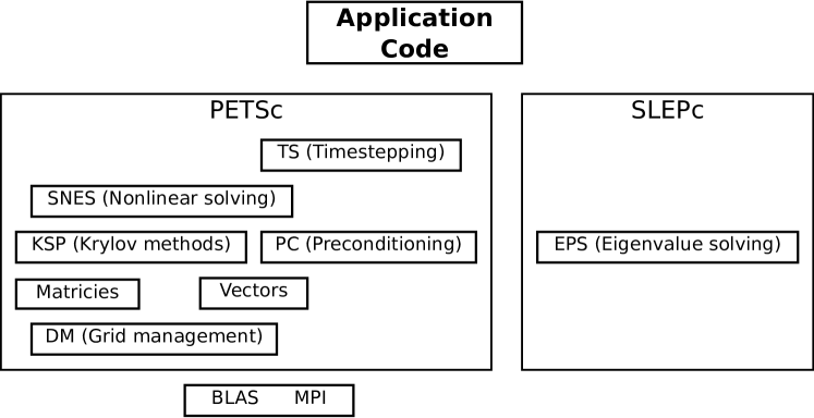
Figure 1: Schematic representation of the components of PETSc and SLEPc used in our code, and their relative hierarchy.

For our dynamical systems calculations we will frequently need to compute specific eigenvalues and eigenvectors for system-sized matrices. For this end, we use SLEPc, which implements iterative eigenvalue solvers using PETSc Vec and Mat distributed data structures. The component of SLEPc that we use is EPS, which has a few algorithms for iteratively solving eigenproblems. Its default algorithm is Krylov-Schur iteration.

2 Model Implementation

2.1 Geometry

Following earlier work by Bojak & Liley (e.g. [11, 19]) we consider the PDEs on a rectangular domain with periodic boundary conditions. On this domain, we use a rectangular grid of $N_{x}$ by $N_{y}$ points. In the tests presented in Sec. 7, the domain and the grid are square. PETSc allows for more complicated domain shapes and grids, that can be encoded in the DM component, independent of the higher-level components.

Within DM, PETSc provides a simpler subcomponent, DMDA, for working with finite differences on structured grids such as our rectangle. If we specify a stencil to use for the spatial derivatives in the DMDA, PETSc will automatically handle numerous things for parallel execution, such as memory allocation and the communication setup for distributed vectors and for the distributed Jacobian matrix.

2.2 Fields

To make use of PETSc’s solvers, the model must be written as a system of equations that is first order in time. This we achieve by introducing new states $J_{jk}$ and $\psi_{ek}$ according to

$$\frac{\partial I_{jk}}{\partial t}=J_{jk}-\gamma_{jk}I_{jk}$$ (6)

$$\frac{\partial J_{jk}}{\partial t}=e\Gamma_{jk}\gamma_{jk}\left\{N^{\beta}_{jk}S_{j}\left[h_{j}\right]+\phi_{jk}+p_{jk}\right\}-\gamma_{jk}J_{jk}$$ (7)

$$\frac{\partial\phi_{ek}}{\partial t}=\psi_{ek}-v^{2}\Lambda^{2}\phi_{ek}$$ (8)

$$\frac{\partial\psi_{ek}}{\partial t}=v^{2}\Lambda^{2}N^{\alpha}_{ek}S_{e}\left[h_{e}\right]+\frac{3}{2}v^{2}\nabla^{2}\phi_{ek}-v^{2}\Lambda^{2}\psi_{ek},$$ (9)

with indices $j,k=\{e,i\}$.

We opted to use a struct, seen in Code. 2.1, to store the fields, rather than a triply indexed array.

typedef struct _Field{
  PetscReal h_e, h_i,
    I_ee, J_ee,
    I_ie, J_ie,
    I_ei, J_ei,
    I_ii, J_ii,
    phi_ee, psi_ee,
    phi_ei, psi_ei;
} Field;

Code 2.1 Struct for the fields.

This allows the code to be more readable in the function and Jacobian evaluation routines. For example, one accesses the $\phi_{ee}$ component at grid point $(x_{i},y_{j})$ simply as u[j][i].phi_ee, provided that the elements of the array (Field **u;) are stored on the processor in which the call is made.

2.3 Parameters

All of the model parameters are stored in a struct designated as the application context. The application context is how PETSc gets problem related parameters into the user-defined functions needed by its solvers.

typedef struct _AppCtx{
  PassiveReal hr_e,  hr_i,
    tau_e, tau_i,
    heq_ee, heq_ie,
    heq_ei, heq_ii,
    Gamma_ee, Gamma_ie,
    Gamma_ei, Gamma_ii,
    gamma_ee, gamma_ie,
    gamma_ei, gamma_ii,
    Nalpha_ee, Nalpha_ei,
    Nbeta_ee, Nbeta_ie,
    Nbeta_ei, Nbeta_ii,
    v, Lambda,
    Smax_e, Smax_i,
    mu_e, mu_i,
    sigma_e, sigma_i,
    p_ee, p_ei,
    p_ie, p_ii;
    ...
} AppCtx;

Code 2.2 Application context struct with the model parameters.

Similar to the fields, this allows readable code for the parameters. For example, one accesses the $\Gamma_{ie}$ parameter as user->Gamma_ie, if user is defined as the pointer AppCtx *user;. How the parameters show up in our struct for the application context is shown in Code 2.2.

2.4 User supplied functions

In addition to the structs listed above, we need to provide PETSc with (at least) a C function that computes the vector field for a given state. We call this function FormFunction, and from this PETSc is capable of approximating the Jacobian with various finite difference methods. However, we also supply a C function to explicitly compute the Jacobian, named FormJacobian, because this allows for more efficient calculations, especially when looking at stepping the variational equations in Sec. 4.

3 Timestepping

We use the implicit Euler method to time-step the discretized equations. As mentioned in Sec. 1.1, this allows us to take larger time steps than feasible with explicit methods. Since we are aiming to compute periodic orbits, rather than to generate long time series, the first order accuracy of the method is not an issue. Once a periodic orbit is computed, the time-step size can be reduced to increase accuracy. Another option is to use Richardson extrapolation to increase the order of accuracy, using the same nonlinear solving as described below.

3.1 Mathematical basis

We symbolically write the dynamical system as

$$\dot{u}=f(u),\quad f:\mathbb{R}^{N}\rightarrow\mathbb{R}^{N}.$$ (10)

where $N$ is the total number of unknowns after discretization, in our case $14\times N_{x}\times N_{y}$. The implicit Euler scheme for time integration is given by

$$u_{n+1}=u_{n}+\mathrm{d}t\,f(u_{n+1})$$ (11)

where the subscript represents the step number, $\mathrm{d}t$ the step size, and $u_{0}$ the initial conditions. This nonlinear equation is solved by Newton iteration:

$$u^{k+1}_{n+1}=u^{k}_{n+1}+\mathrm{d}u^{k},$$ (12)

where the superscript denotes the Newton iterate, and $\mathrm{d}u^{k}$ is the solution to the linear system

$$\left(\mathbb{I}-\mathrm{d}t\left.\frac{\partial f}{\partial u}\right|_{u^{k}_{n+1}}\right)\mathrm{d}u^{k}=\mathrm{d}t\,f(u^{k}_{n+1})-u^{k}_{n+1}+u^{k}_{n},$$ (13)

where $\partial f/\partial u$ denotes the $N\times N$ Jacobian matrix. Provided that the initial approximation, $u^{0}_{n+1}$, is close enough to the actual solution of equation (11), this iteration should converge quadratically. This is achieved by making the initial approximation the result of an explicit Euler step

$$u^{0}_{n+1}=u_{n}+\mathrm{d}t\,f(u_{n}).$$ (14)

As we scale up the size of our problems, it becomes the linear solve in equation (13) that takes most time. This problem is handled by using GMRES to solve the linear system. For large time steps, the spectrum of the matrix in Eq. 13 is spread out, and we need to precondition it for iterative solving. We make use ILU, which has shown to be reliable [25, 26] for this type of problem. If we use more than one processor, PETSc uses distributed storage for the matrix, and combines ILU with block Jacobi preconditioning.

3.2 Implementation

PETSc provides a simple interface for timestepping in its TS component. The basic code required to set up a TS is given in Code 3.1. With a TS set up like this, the timestepping parameters are set from command line arguments at run time. For example, to do implicit Euler timestepping for $40.67\,\mathrm{ms}$ with a time step of $0.1\,\mathrm{ms}$, one needs to provide the arguments
-ts_type beuler -ts_dt 0.1 -ts_final_time 40.67.
In this specific case, since the final time is not an integer number of timesteps, PETSc will step past it, and interpolate at the desired time.

  TS     ts;
  TSCreate(PETSC_COMM_WORLD,&ts);
  TSSetProblemType(ts,TS_NONLINEAR);
  TSSetExactFinalTime(ts);
  TSSetRHSFunction(ts,PETSC_NULL,FormFunction,&user);
  TSSetRHSJacobian(ts,J,J,FormJacobian,&user);
  TSSetFromOptions(ts);
  TSSolve(ts,u,PETSC_NULL)

Code 3.1 PETSc code for setting up and running the timestepping. FormFunction and FormJacobian are user provided functions that compute the rhs of equation (10), and its Jacobian respectively. J is an appropriately allocated matrix to hold the Jacobian, and u a vector to hold the solutions.

4 Stepping of the variational equations

4.1 Mathematical basis

The variational equations for the dynamical system are written as

$$\dot{v}=\left.\frac{\partial f}{\partial u}\right|_{u}v,\quad v\in\mathbb{R}^{N}$$ (15)

and must be integrated simultaneously with the dynamical system (10). Solving the variational equations allow us to compute the stability of solutions, and is also an essential ingredient for the treatment of boundary value problems such as those that arise in the computation of periodic orbits.

Performing implicit Euler timestepping on the variational equations (15) requires solutions of the linear problems

$$\left(\mathbb{I}-\mathrm{d}t\left.\frac{\partial f}{\partial u}\right|_{u_{n+1}}\right)v_{n+1}=v_{n}.$$ (16)

Since we already have the Jacobian of the dynamical system at timestep $n+1$, stepping the variational equations requires only one additional $N\times N$ linear solve per time step.

4.2 Implementation

In PETSc, we implement the timestepping of the variational equations as a MATSHELL. A MATSHELL allows users to define their own matrix type. Within a MATSHELL, one needs to give a context for storing the relevant data and write functions for the desired matrix operation. For example, we point the operation MATOP_MULT to a function that takes the initial state of the variational system $v(0)$ as input, and outputs the result $v(T)$ at the end of the timestepping. The context we use for the time stepping of the variational equations is shown in Code 4.1. The function we provide for MATOP_MULT works by first taking a step of the TS, then loading the Jacobian computed from that step and solving equation (16). This is repeated until the TS reaches its end.

typedef struct _PeriodIntegrationCtx{
  // timestepping of the original eqn
  TS      ts;
  Mat     tsJac;
  Vec     initState,endState,fullSol;
  // additional requirements for variational eqn
  Mat     J,eye;
  KSP     ksp;
} PeriodIntegrationCtx;

Code 4.1 The MATSHELL context for timestepping of the variational equations. The TS holds the relevant info for stepping the dynamical system

The MATSHELL thus defined can be used by SLEPc for the iterative computation of eigen pairs. In particular, we will use this approach to compute the Floquet multipliers of periodic orbits.

5 Equilibria

Having set up the function FormFunction for the right hand side of the dynamical system, and its Jacobian computation FormJacobian, also used for time integration, we can set up equilibrium calculations using PETSc’s SNES component with very little effort.

5.1 Mathematical Basis

Equilibrium solutions to the dynamical system (10) are solutions that satisfy

$$f(u)=0.$$ (17)

To solve this, we can set up a Newton iteration scheme

$$u^{k+1}=u^{k}+\mathrm{d}u^{k}$$ (18)

with $\mathrm{d}u$ coming from the solution of the linear system

$$\left.\frac{\partial f}{\partial u}\right|_{u^{k}}\mathrm{d}u^{k}=-f(u^{k}).$$ (19)

As with the timestepping, if the initial guess is good enough this will converge quadratically provided that $\left.\frac{\partial f}{\partial u}\right|_{u^{k}}$ is nonsingular. Unlike the case of time stepping, though, we do not always have a way to produce an initial approximation that is good enough. For stable equilibrium solutions, we can use timestepping to get close to an equilibrium, but this will not work for unstable equilibria. One possible solution is using globally convergent Newton methods. Using such methods we can find equilibria from very coarse initial data, at the cost of computing many iterations. The line search algorithm and the trust region approach (see, e.g. [24]) are implemented in the SNES component.

Stability of equilibrium solutions follows from the spectrum of the Jacobian. Because of the spatial symmetries of the model, these will mostly appear in groups. On a square domain, for instance, a single eigenvalue will be associated with up to eight eigenvectors, with wavenumbers $(\pm k_{x},\pm k_{y})$ and $(\pm k_{y},\pm k_{x})$.

5.2 Implementation

Setting up and using a nonlinear solver within PETSc is straightforward, as shown in Code 5.1. The default algorithm used by SNES is Newton’s method with line search.

  SNES    snes;
  SNESCreate(PETSC_COMM_WORLD,&snes);
  SNESSetFunction(snes,r,FormFunctionSNES,&user);
  SNESSetJacobian(snes,J,J,FormJacobianSNES,&user);
  SNESSetFromOptions(snes);
  SNESSolve(snes,PETSC_NULL,u);

Code 5.1 Code snippet for solving for equilibria. Vectors r and u are preallocated, with u being the initial approximation, and J a preallocated matrix for the Jacobian.

6 Periodic solutions

The primary instability in the Liley model is often a Hopf bifurcation, and periodic orbits have been shown to play an important role in the dynamics of ODE reductions of the model (e.g. [14, 27]). However, space dependent periodic orbits have not previously been computed and studied. Using PETSc data structures for bordered matrices, in conjunction with a MATSHELL structure, we can solve for periodic orbits based on the time stepping described in Secs. 3 and 4.

6.1 Mathematical basis

Periodic orbits solve the boundary value problem

$$F(u,T)=\phi(u,T)-u=0,$$ (20)

where $\phi$ is the flow of the dynamical system (10), and $T$ is the period. Our strategy for solving this equation is essentially that of Sanchez et al. [28], namely Newton iterations combined with unconditioned GMRES iteration. Linearising Eq. 20 gives

$$\left(D_{u}\phi(u,T)-\mathbb{I}\right)\mathrm{d}u+f(\phi(u,T))\mathrm{d}T=-F(u,T),$$ (21)

where $D_{u}\phi$ is a matrix of derivatives of the flow with respect to its initial condition. Upon convergence, this is the monodromy matrix of the periodic orbit. This results in $N$ equations in $N+1$ unknowns, which must be closed by a phase condition. We opted for the use of a Poincaré plane involving one of the state variables, $u_{k}$:

$$\phi_{k}(u,T)-C=0,$$ (22)

where $C$ is set appropriately, for instance to the time-mean value of $u_{k}$. This choice gives the following bordered system

$$\left[\begin{array}[]{cc}\left(D_{u}\phi(u,T)-\mathbb{I}\right)&f(\phi(u,T))\\ \left[D_{u}\phi(u,T)\right]_{k,.}&f_{k}(\phi(u,T))\end{array}\right]\left[\begin{array}[]{c}\mathrm{d}u\\ \mathrm{d}T\end{array}\right]=\left[\begin{array}[]{c}-F(u,T)\\ C-\phi_{k}(u,T)\end{array}\right],$$ (23)

where $[D_{u}\phi(u,T)]_{k,.}$ denotes the $k^{\rm th}$ row of the matrix $D_{u}\phi$. An update can then be made to the approximate solution as

$$\left[\begin{array}[]{c}u^{n+1}\\ T^{n+1}\end{array}\right]=\left[\begin{array}[]{c}u^{n}\\ T^{n}\end{array}\right]+\left[\begin{array}[]{c}\mathrm{d}u\\ \mathrm{d}T\end{array}\right].$$ (24)

The matrix $D_{u}\phi$ is dense, so we should avoid calculating and storing it explicitly. Iterative solving of the linear problem, (23), requires the computation of matrix-vector products, which are constructed from the integration of the variational equation (15) with $v=\mathrm{d}u$ and the vector field $f(\phi(u,T))$ at the end point of the approximately periodic orbit. Since the governing PDE is dissipative, most of the eigenvalues of the monodromy matrix are clustered around zero. This aids the convergence of GMRES, without any preconditioning. Sanchez et al. [28] provide bounds for the number of GMRES iterations for the Navier-Stokes equation, and the convergence we observe for the Liley model is qualitatively similar.

6.2 Implementation

The problem of creating a bordered matrix system in a distributed environment is not a trivial one. The specific case that we have is one vector, $u$, that is sparsely connected and distributed among processors, and one parameter, $T$, that must exist and be synchronized across all processors.

PETSc’s DM module has some recently introduced functionality that allows us to handle this in a straightforward way, letting us make use of the DMDA already used in the other types of calculations.

DMRedundant can be used for the $T$ component of our extended system, as it has the precise behaviour that we require. Next, we use a DMComposite to join together the DMDA of the grid with the DMRedundant of the period. We can then derive vectors from this DMComposite, and use these vectors for PETSc’s iterative linear solvers. PETSc code that illustrates this idea is shown in Code 6.1.

  DM  packer, redT;
  DMCompositeCreate(PETSC_COMM_WORLD,&packer);
  DMRedundantCreate(PETSC_COMM_WORLD,0,1,&redT);
  DMCompositeAddDM(packer,da);
  DMCompositeAddDM(packer,redT);

Code 6.1 Additional DM pieces for extended vectors as in equation (24), assuming that da is the DM associated with the grid structure. The numerical arguments in DMRedundantCreate represent the processor where the redundant entries live (in global vectors), and the number of redundant entries respectively.

The matrix multiplication is done through a MATSHELL, and the struct that holds the relevant data is found in Code 6.2.

typedef struct _PeriodFindCtx{
  Mat          *linTimeIntegration;
  DM           packer,redT;
  Vec          endState,f_at_endState;
} PeriodFindCtx;

Code 6.2 For finding periodic solution, we need a method for integrating the variational equations (the MATSHELL discussed in section 4), additional DMs, and space for holding $f$ evaluated at the state at the end of the integration

7 Example calculations

In this section, we present some computations that serve to validate our implementation and to investigate its efficiency. All tests are based on the parameter set in Table 1, and the scaling of the number of local inhibitory-to-inhibitory connections, $r$, is varied around the first bifurcation from an equilibrium to more complicated, spatio-temporal behaviour.

Fig. 2 shows the neutral stability curve for the spatially homogeneous equilibrium, which is the unique attractor of the model at small values of $r$. The primary transition is a Hopf bifurcation with spatial wave numbers that depend on the system size. For systems smaller than $2\times 2\,\mathrm{cm}^{2}$, the emerging periodic orbit is spatially homogeneous. For larger systems, space dependent orbits emerge, and their typical length scale converges to about $9.3\,\mathrm{cm}$ for large system sizes. These stability curves were computed by solving small eigenvalue problems for each combination of wavenumbers, independent from the PETSc implementation. The eigenvalues computed by Krylov-Schur iteration in SLEPc, presented in Sec. 7.2, are in good agreement.

A partial bifurcation diagram, for spatially homogeneous solutions only, is shown in Fig. 3. In this diagram, the Hopf bifurcation is subcritical, and time series analysis indicates that the Hopf bifurcations associated with nonzero wave numbers are, too. The time series presented in Sec. 7.1 was generated by starting from the equilibrium at $r=1$ and adding a finite-size perturbation in the least stable direction, with wave number $|k_{x}|=|k_{y}|=1$.

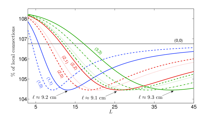
Figure 2: Neutral stability curve for the spatially homogeneous equilibrium of the Liley model with parameters set according to Table 1. Shown is the scaling parameter, $r$, versus the linear domain size, $L$, and wave numbers $\bm{k}=(k_{x},k_{y})$ are shown in parenthesis. When varying $r$, only for very small domains the primary instability is spatially homogeneous. For domain sizes over $12.5\times 12.5\text{cm}^{2}$ the location of the primary instability approaches $r=1.04$ and the length scale of the leading instability approaches $L/\|\bm{k}\|=9.3\,\mathrm{cm}$.

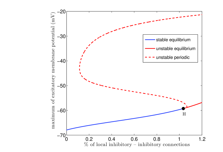
Figure 3: Partial bifurcation diagram showing the primary transition from a spatially homogeneous equilibrium to a space and time dependent periodic orbit. On the vertical axis the scaling parameter $r$ is plotted, and on the vertical axis the (maximum of) the excitatory membrane potential. The branch of periodic solutions shown with a dashed line is a spatially homogeneous branch that is unstable to space-dependent perturbations.

7.1 Timestepping

For the timestepping demonstration, we used a system size of $12.8\times 12.8\,\mathrm{cm}^{2}$ with $0.5\,\mathrm{mm}$ resolution, resulting in a $256\times 256$ grid, and $N=917,504$ unknowns in total. Setting the parameter $r=1.0$, we initialize with the stable equilibrium solution perturbed by its least stable eigenmode, shown in Fig. 7. Since the equilibrium solution is stable, small perturbations just decay, but sufficiently large perturbations grow. The snapshots of Fig. 4 were taken after a transient time of 600ms. The membrane potentials show behaviour that is nearly periodic, with a dominant period of 40Hz, as demonstrated by the power spectrum shown in the last panel.

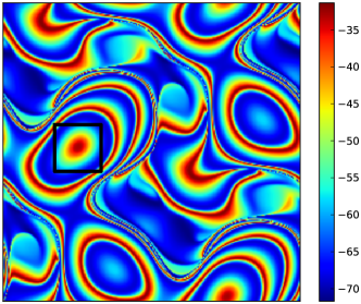
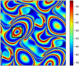
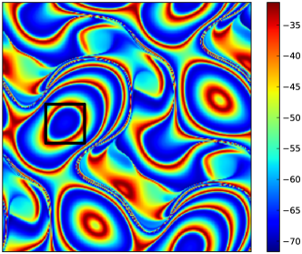
Figure 4: Three snapshots of the excitatory membrane potential, $6\,\mathrm{ms}$ apart, of a solution at $r=1$, near the primary Hopf bifurcation. The domain size is $12.8\times 12.8\,\mathrm{cm}^{2}$, the resolution is $0.5\,\mathrm{mm}$ and the time-step size $1\,\mathrm{ms}$. The fourth panel shows the power spectrum of $h_{e}$, averaged over the region inside the black square.

Since the time-stepping code lies at the core of the periodic orbit solver, we carefully investigated its scaling with an increasing number of processors. Doubling the domain size, while keeping the grid spacing fixed, gives a dynamical system with $N=3,670,016$ degrees of freedom. We time-stepped this system on a small subcluster of $2.4\,\mathrm{GHz}$ AMD Opteron nodes with gigabit interconnects. Apart from some minor load-balancing effects, the scaling is linear up to 16 processors, despite the relatively slow interconnects.

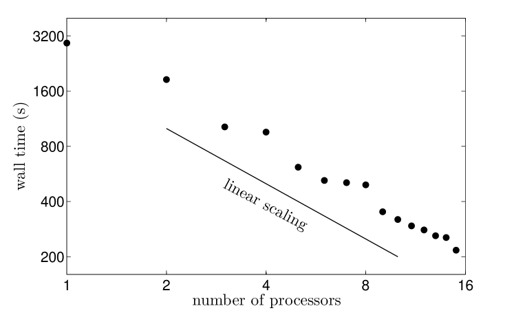
Figure 5: Wall time for the computation of 50 time steps of $1\,\mathrm{ms}$ each on a $25.6\times 25.6\,\mathrm{cm}^{2}$ domain with $0.5\,\mathrm{mm}$ resolution. The fully implicit Euler steps are computed with Newton iterations, each of which is solved for by GMRES, preconditioned with a combination of block Jacobi and ILU. The initial guess is given by an explicit Euler step. Two or three Newton iterations are sufficient to reduce the residual by a factor of $10^{8}$. About 80 Krylov vectors are computed by GMRES to bring the relative residual down to $10^{-5}$. The number of unknowns is $N=3,670,016$.

7.2 Equilibrium

We computed the whole equilibrium curve of Fig. 3 through parameter continuation, which is a trivial extension of the algorithm for computing equilibria, presented in Sec. 5. For each computed equilibrium solution, we took the Jacobian and used SLEPc to compute the eigenvalues with the largest real parts. The result is shown in Fig. 7. As predicted by the neutral stability curve computation, the $(1,1)$ mode turns unstable first, immediately followed by the $(1,0)$ mode. Around $r=1.08$, the $(0,2)$ mode crosses the $(0,1)$ mode and proceeds to become the most unstable mode for larger values of $r$. The least stable eigenmode for $r=1.046$, just after its eigenvalue has crossed zero, is shown in Fig. 7.

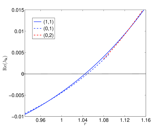
Figure 6: The real parts of the leading two eigenvalue pairs of the spatially homogeneous equilibrium tracked in the scaling parameter $r$, for system size $L=12.8\,\mathrm{cm}$. The primary transition is tied to wave numbers $|k_{x}|=|k_{y}|=1$. The other curves shown are for wave numbers $k_{x}=0$, $k_{y}=\pm 1$ and $k_{x}=\pm 1$, $k_{y}=0$ and for $k_{x}=0$, $k_{y}=\pm 2$ and $k_{x}=\pm 2$, $k_{y}=0$.

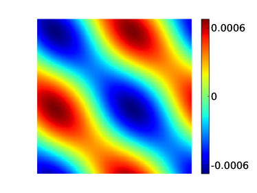
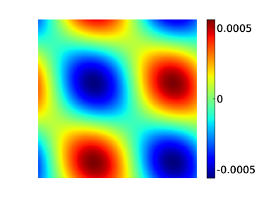
Figure 7: The real part of the least stable eigenmode of the stable equilibrium located at $r=1.046$. Displayed are the excitatory (left) and inhibitory (right) membrane potentials. The eigenvector, with wave numbers $(1,1)$, was computed by Arnoldi iteration and is scaled to have unit $L_{2}$ norm.

7.3 Periodic solutions

We tested the computation of periodic orbits on a smaller grid, namely $16\times 16$ points, still with $0.5\,\mathrm{mm}$ resolution, and with $r=1.2$. The primary Hopf bifurcation is sub critical, so there is no easy way to compute the branch of space-dependent periodic solutions. Instead, we computed one of the spatially homogeneous orbits, for which an approximate solution can readily be obtained from analysis of the ODE reduction of the model. In fact, the upper part of the branch of periodic orbits shown in Fig. 3 is stable to all spatially homogeneous perturbations.

Figure 8: Residuals of the Newton iteration (left) and the corresponding GMRES iterations (right). The latter is normalised by the norm of the right hand side of Eq. 23, i.e. the Newton residual. The tolerance was set at $10^{-8}$ for the Newton iteration and to $10^{-5}$ for the GMRES iteration. Note the super linear convergence of the former.

Starting from a coarse initial approximation, the Newton iterations converged faster than linear, and each Newton step took between 8 and 11 GMRES iterations, out of a maximum of $N+1=3585$. Subsequently, we computed the most unstable multipliers, using SLEPc with the MATSHELL that computes products with the bordered matrix, as described in Sec. 6.2. The most unstable multiplier is $\mu_{1}=1.111$ and corresponds to a wave number $(1,1)$ perturbation.

8 Conclusion and future improvements

In the current paper, we have presented the basic implementation of the model and example computations to validate it and test its performance. The code will be available publicly [16]. As it is built on top of PETSc, the user has access to a range of nonlinear and linear solvers and preconditioners, which can be used to solve the boundary value problems that typically arise in dynamical systems analysis. The periodic orbit computation, presented in Sec. 7.3, is a simple example of such a boundary value problem, that has all the ingredients: a module for time-stepping the system and perturbations and a representation of user-specified, bordered matrices.

The next step in the development of the code is the implementation of pseudo-arclength continuation of equilibria and periodic orbits. This will enable us, for instance, to complement the bifurcation diagram of the current test case, Fig. 3, with the branches of space-dependent periodic solutions that actually regulate the observed dynamics, in contrast to the highly unstable spatially homogeneous periodic orbits computed from an ODE reduction of the model.

We expect that our implementation will be useful to researchers studying the dynamics of the Liley model, or similar models, such as the model with gap junctions proposed by Steyn-Ross et al. [18]. Also, it could be useful for those who incorporate a similar mean-field model in, for instance, the control of robotic motion or network models of brain activity.

References

- [1] E. Izhikevich, G. Edelman, Large-scale model of mammalian thalamocortical systems, PNAS 105 (2008) 3593–3598.
-
[2]
The blue brain project.
URL http://bluebrain.epfl.ch/ - [3] P. Nunez, R. Srinivasan, Electric Fields of the Brain. The Neurophysics of EEG, 2nd Edition, Oxford University Press, Oxford, 2006.
- [4] W. Freeman, Mass action in the nervous system, Academic Press, New York, 1975.
- [5] H. R. Wilson, J. D. Cowan, Excitatory and inhibitory interactions in localized populations of model neurons, Biophys. J. 12 (1972) 1–24.
- [6] F. Lopes da Silva, A. Hoeks, H. Smits, L. Zetterberg, Model of brain rhythmic activity, Kybernetik 15 (1974) 27–37.
- [7] P. Nunez, The brain wave equation: A model for the EEG, Math. Biosci. 21 (1974) 279–297.
- [8] M. Breakspear, J. Roberts, J. Terry, S. Rodrigues, M. N, P. Robinson, A unifying explanation of primary generalized seizures through nonlinear brain modeling and bifurcation analysis, Cereb. Cortex 16 (2006) 1296–1313.
- [9] M. Kramer, A. Szeri, J. Sleigh, H. Kirsch, Mechanisms of seizure propagation in a cortical model, J. Comput. Neurosci. 22 (2007) 63–80.
- [10] A. Blenkinsop, A. Valentin, M. Richardson, J. Terry, The dynamic evolution of focal-onset epilepsies – combining theoretical and clinical observations, Eur. J. Neurosci. 36 (2012) 2188–2200.
- [11] I. Bojak, D. Liley, Modeling the effects of anesthesia on the electroencephalogram, Phys. Rev. E 71 (2005) 1–22.
- [12] J. Quinton, B. Girau, Spatiotemporal pattern discrimination using predictive dynamic neural fields, BMC Neurosci. 13 (Suppl. 1 (O16)).
- [13] D. T. J. Liley, P. J. Cadusch, M. P. Dafilis, A spatially continuous mean field theory of electrocortical activity, Network-Comput. Neural 13 (2002) 67–113.
- [14] F. Frascoli, L. van Veen, I. Bojak, D. Liley, Metabifurcation analysis of a mean field model of the cortex, Physica D 240 (2011) 949–962.
- [15] S. Balay, J. Brown, K. Buschelman, V. Eijkhout, W. D. Gropp, D. Kaushik, M. G. Knepley, L. M. Curfman, B. F. Smith, H. Zhang, PETSc Users Manual, Tech. rep., Argonne National Laboratory (2012).
-
[16]
Source code available from.
URL http://faculty.uoit.ca/vanveen/MFM/ - [17] S. Coombes, P. Graben, R. Potthast, J. J. Wright (Eds.), Neural Field Theory, Springer Verlag, 2012, Ch. Spots: breathing, drifting and scattering in a neural field model.
- [18] M. L. Steyn-Ross, D. A. Steyn-Ross, J. W. Sleigh, M. T. Wilson, A mechanism for ultra-slow oscillations in the cortical default network, Bull. Math. Bio. 73 (2011) 398–416.
- [19] I. Bojak, D. Liley, Self-organized 40Hz synchronization in a physiological theory of EEG, Neurocomputing 70 (2007) 2085–2090.
-
[20]
S. Balay, J. Brown, K. Buschelman, W. D. Gropp, D. Kaushik, M. G. Knepley,
L. M. Curfman, B. F. Smith, H. Zhang,
PETSc Web page (2012).
URL http://www.mcs.anl.gov/petsc - [21] V. Hernandez, J. E. Roman, V. Vidal, SLEPc: A scalable and flexible toolkit for the solution of eigenvalue problems, ACM T. Math. Software 31 (3) (2005) 351–362.
- [22] Y. Saad, M. H. Schultz, GMRES: A generalized minimal residual algorithm for solving nonsymmetric linear systems, SIAM J. Sci. Stat. Comput. 7 (1986) 856–869.
- [23] Y. Saad, Iterative Methods for Sparse Linear Systems, 2nd Edition, SIAM, 2003.
- [24] J. E. Dennis, R. B. Schnabel, Numerical Methods for Unconstrained Optimization and Nonlinear Equations, SIAM, 1996.
- [25] J. Sanchez, F. Marques, J. M. Lopez, A continuation and bifurcation technique for Navier–Stokes flows, J. Comput. Phys. 180 (2002) 78–98.
- [26] Y. Saad, Preconditioned Krylov subspace methods for CFD applications, Tech. rep., Minnesota Supercomputer Institute, Minneapolis (1994).
- [27] L. van Veen, D. Liley, Chaos via Shilnikov’s saddle-node bifurcation in a theory of the electroencephalogram, Phys. Rev. Lett. 97 (2006) 208101.
- [28] J. Sanchez, M. Net, B. Garcia-Archilla, C. Simó, Newton–Krylov continuation of periodic orbits for Navier–Stokes flows, J. Comput. Phys. 201 (2004) 13–33.