Modulated pulses compensating classical noise

Abstract

We consider pulses of finite duration for coherent control in the presence of classical noise. We derive the corrections to ideal, instantaneous pulses for the case of general decoherence (spin-spin relaxation and spin-lattice relaxation) up to and including the third order in the duration $\tau_{\text{p}}$ of the pulses. For pure dephasing (spin-spin relaxation only), we design $\pi$ and $\pi/2$ pulses with amplitude and/or frequency modulation which resemble the ideal ones up to and including the second order in $\tau_{\text{p}}$. For completely general decoherence including spin-lattice relaxation the corrections are computed up to and including the second order in $\tau_{\text{p}}$ as well. Frequency modulated pulses are determined which resemble the ideal ones. They are used to design a low-amplitude replacement for XY8 cycles. In comparison with pulses designed to compensate quantum noise less conditions have to be fulfilled. Consequently, we find that the classical pulses can be weaker and simpler than the corresponding pulses in the quantum case.

1 Introduction

In open quantum systems the interaction with an environment is one of the main reasons for the decay of the coherence and for the loss of information, both obstacles to an efficient processing of quantum information or to high precision NMR measurements. But by means of a proper time-dependent modulation of the system dynamics, it is possible to average out the effects of the environment. This leads to the prolongation of the coherence time and to the suppression of the decoherence.

In NMR, a standard way of time-dependent modulation is the application of very short pulses which flip spins. This approach dates back to the spin echo of Erwin Hahn in the fifties [1] and then was quickly extended to periodically applied pulses by Carr and Purcell [2] and Meiboom and Gill [3]. Since then a large variety of periodic pulse sequences has been proposed [4, 5] among which we highlight the XY4 cycle [6, 7] and its derivatives as a means to preserve all three spin directions.

Recently, the approach of stroboscopic pulsing of two-level systems to suppress their decoherence has been revived under the name of dynamic decoupling (DD) for open quantum systems in the context of quantum information processing (QIP) [8, 9, 10]. Again, the idea is to effectively decouple the two-level system from the environment which induces its decoherence. Interestingly, quantum information processing requires a slightly differing performance than NMR. During the information processing it is desired that the decoherence is much better suppressed to the level of $10^{-2}$ to $10^{-4}$. But deviations at longer times do not matter. In contrast, in NMR a loss of signal of the order of 50% still allows one to track the signal, but it is desired to be able to do this for as long as possible.

Hence, in QIP novel sequences of pulses have been recently developed which do not rely on periodically repeated cycles, but vary the time intervals between the pulses. A first suggestion relies on recursively concatenated sequences (CDD). They require an exponentially growing number of pulses [11] if longer times have to be reached. For the suppression of dephasing (spin-spin relaxation) the Uhrig dynamic decoupling (UDD) is much more efficient because it requires only a linearly growing number of pulses [12, 13, 14, 15]. In practice, this pays for power spectra with hard cutoff [16, 14, 17]. Subsequently, UDD has been extended to also suppress general decoherence including spin-lattice relaxation due to spin flips. This sequence goes under the name of quadratic dynamic decoupling (QDD) [18, 19, 20, 21] and it is further generalized to nested UDD to deal with more than one two-level system, i.e., with quantum registers [22]. Experimental verification of these theoretical proposals are also available for the UDD [23, 24].

All the above approaches rely theoretically on ideal, instantaneous pulses which can not be realized experimentally. There are various routes to overcome this problem. One is to abandon the use of pulses altogether by resorting to continuous control fields, see for instance Ref. [25]. We will not follow this route here but stick to sequences of pulses. We point out, however, that there is a crossover between both approaches if the pulses become so long that one touches the next one or if a pulse is designed such that it acts itself like a cycle of pulses, see below.

For pulses, the most direct solution is to realize very short pulses so that their duration $\tau_{\text{p}}$ is so short that the coupling to the bath does not play a role during the pulse

$$U_{\text{p}}\left(\tau_{\text{p}},0\right)=\hat{P}_{\tau_{\text{p}}}+{\cal O}(\tau_{\text{p}})$$ (1)

where $U_{\text{p}}\left(\tau_{\text{p}},0\right)$ is the unitary time evolution under the combined action of the coupling between system (spin, qubit, or two-level system) and bath as well as the coherent control while $\hat{P}_{\tau_{\text{p}}}$ stands for the time evolution under the pulse alone as if the system were isolated.

A more sophisticated solution consists in shaping the pulse such that the above approximation holds in the form

$$U_{\text{p}}\left(\tau_{\text{p}},0\right)=\hat{P}_{\tau_{\text{p}}}+{\cal O}(\tau_{\text{p}}^{m+1}).$$ (2)

We will call a pulse which fulfills (2) an $m$-th order pulse. Thus, a standard unshaped pulse is a 0-th order pulse. In this work, we will present first and second order pulses.

We emphasize that pulses with the property (2) cannot be used as simple replacements for an ideal, instantaneous pulse because they still last for the time $\tau_{\text{p}}$. A proper replacement would have to fulfill

$$U_{\text{p}}\left(\tau_{\text{p}},0\right)=U\left(\tau_{\text{p}},\tau_{\text{id}}\right)\hat{P}_{\tau_{\text{p}}}U\left(\tau_{\text{id}},0\right)+{\cal O}(\tau_{\text{p}}^{m+1})$$ (3)

where $U\left(\tau_{2},\tau_{1}\right)$ is the unitary time evolution without any external control and $\tau_{\text{id}}$ is the instant at which the $\delta$-like control pulse $\hat{P}_{\tau_{\text{p}}}$ is inserted. The time evolutions $U$ before and after an ideal, instantaneous pulse $\hat{P}_{\tau_{\text{p}}}$ simulate that right before and after an ideal pulse the system is coupled to its decohering environment. It could be shown, however, that for $\pi$ pulses the ansatz (3) can at most be fulfilled for $m\leq 1$ so that the route of finding proper replacements cannot be pursued further [26, 27].

Hence, the ansatz (2) had to be developed further because it can be realized for arbitrary $m$ in principle [28] and concrete proposals have recently been made for second order pulses ($m=2$) for general quantum baths [29, 30]. It could be shown that pulses with this property can be used in sequences of pulses if they are not used in the same manner as instantaneous pulses would be used, but with adapted sequences [31, 32]. These observations clearly show that the shaping of pulses is an important ingredient for high-fidelity coherent control.

Of course, shaping of pulses has also been a long-standing issue in NMR. The main aim was to generate robust pulses which are only weakly susceptible to pulse imperfections. We can mention only partly the abundant literature on this issue [33, 34, 35, 36, 37, 38, 39, 40, 41, 42, 43], for a book see Ref. [44].

In contrast to earlier work, e.g., the one by Skinner and collaborators [37, 38], we focus in this article on analytical derivations as far as possible. In contrast to our previous work on pulses for systems coupled to quantum baths [29, 30] we will discuss classical baths. The fundamental reason is that in most experiments the dominating fluctuations destroying coherence are of classical nature, see, e.g., Ref. [45]. Generically the decohering fluctuations are induced by a large number of microscopic and macroscopic degrees of freedom. These degrees of freedom are at least partly at rather high temperatures relative to their generic energy scales. For instance, the nuclear spins can mostly be considered to be in a disorderd state corresponding to infinite temperature. Thus the resulting fluctuations are thermal fluctuations and their quantum character plays only a smaller role.

One may think that the strongly disordered states of the decohering baths pose a problem to the preservation of coherence in the systems under study. But the opposite is true: The lack of quantumness of the fluctuations allows us to consider classical fluctuations only. This implies less restrictive conditions on $m$-th order pulses of the type (2). Hence, the necessary pulse shapes are simpler and most importantly the required amplitudes are lower than in the full quantum case. The main goal of the present article is to show this explicitly. The concomitant message to experiment is that for given power supply the classical pulses will be easier to realize. They can be made shorter than their quantum analogues.

In this article, we derive amplitude and frequency modulated pulses for pure dephasing due to classical noise, i.e., for spin-spin relaxation without spin flips, up to and including second order ($m=2$). Particular attention will be paid to the minimization of the amplitude because this is important for practical use. For general decoherence due to classical noise, i.e., including spin flips due to spin-lattice relaxation, we derive frequency modulated pulses up to and including second order ($m=2$). We stress that such pulses can be used to build continuous versions of the well-known XY8 cycle [6, 7].

The paper is organized as follows: In section 2 the equations for the decoupling of general decoherence are derived. In sections 3 and 4 these equations are shown for the first and second order. They are solved numerically for the case of pure dephasing, both for amplitude and for frequency modulated pulses. In section 5 we study decoupling pulses that combine the characteristics of amplitude (AM) and frequency modulation (FM) in order to illustrate that transient amplitudes, when the pulse is switched on or off, can be easily dealt with. In section 6 the case of general decoherence is solved for by frequency modulated pulses. We draw our conclusions in section 7.

2 General Equations

2.1 Ansatz

We consider the following Hamiltonian

$$H_{\text{tot}}\left(t\right)=H\left(t\right)+H_{0}\left(t\right)$$ (4)

which consists of two parts: A system Hamiltonian

$$H\left(t\right)=\vec{\eta}\left(t\right)\cdot\vec{\sigma}$$ (5)

and a control Hamiltonian

$$H_{0}\left(t\right)=\vec{v}\left(t\right)\cdot\vec{\sigma}.$$ (6)

The system Hamiltonian describes the physics of a single spin coupled to a classical bath through the time-dependent random function $\vec{\eta}(t)$. We describe decoherence by averaging over $\vec{\eta}(t)$. One may assume $\vec{\eta}(t)$ to represent Gaussian fluctuations, but this is not essential for the present work. The vector $\vec{\sigma}$ with components given by the Pauli matrices $\sigma_{x}$, $\sigma_{y}$ and $\sigma_{z}$ stands for the spin operator. The spin is subject to general dephasing including spin-lattice relaxation if all three vector components are present.

In the control Hamiltonian $H_{0}(t)$, $\vec{v}(t)$ is the time-dependent vector-valued amplitude of the pulse operating on the spin. At each instant in time, the spin undergoes a rotation about the time-dependent axis $\vec{v}(t)$.

In all what follows we assume that the control $|\vec{v}|$ is large enough $\pi\approx\vec{v}\tau_{\text{p}}$ so that $\tau_{\text{p}}$ can be chosen small enough and $\pi\gtrapprox\|H_{0}\|\tau_{\text{p}}$ holds. Then it is well justified to expand in the decoherence dynamics. Formally, we perform an expansion in $\tau_{\text{p}}$ while $|\vec{v}|\tau_{\text{p}}$ is kept at order unity.

Following the technique developed in Refs. [29, 30] we split the complete time-evolution operator $U_{\text{p}}\left(\tau_{\text{p}},0\right)={\cal T}\left\{\exp[-i\int\limits_{0}^{\tau_{\text{p}}}H_{\text{tot}}\left(t\right)\mathrm{dt}]\right\}$ of the system during a pulse of duration $\tau_{\text{p}}$ into two terms: (i) The evolution of the spin under the effect of only the control field $\hat{P}_{\tau_{\text{p}}}$ – as if it were decoupled from the bath – and (ii) the correction $U_{\text{c}}\left(\tau_{\text{p}},0\right)$

$$U_{\text{p}}\left(\tau_{\text{p}},0\right):=\hat{P}_{\tau_{\text{p}}}U_{\text{c}}\left(\tau_{\text{p}},0\right).$$ (7)

The notation $\cal T$ stands for the quantum mechanical time-ordering operator. The operator $U_{\text{c}}\left(\tau_{\text{p}},0\right)$ incorporates the deviations from an ideal rotation resulting from the interaction between the spin and the bath.

The rotation operator can be expressed as

$$\hat{P}_{t}:=\exp\{-i\vec{\sigma}\cdot\vec{a}(t)\frac{\psi(t)}{2}\},$$ (8)

where the unit vector $\vec{a}$ stands for the axis of total rotation while $\psi(t)$ is the corresponding angle by which the spin is rotated from the instant $\tau=0$ till the instant $\tau=t$.

Both operators $\hat{P}_{t}$ and $U_{\text{p}}\left(t,0\right)$ satisfy a Schrödinger equation at every instant $t$, for details see Ref. [29, 30]. For the former operator $i\partial_{t}\hat{P}_{t}=H_{0}(t)\hat{P}_{t}$ translates to

$$2\vec{v}(t) =\psi^{\prime}(t)\hat{a}(t)+\hat{a}^{\prime}(t)\sin\psi(t)$$

$$-(1-\cos\psi(t))\left[\hat{a}^{\prime}(t)\times\hat{a}(t)\right].$$ (9)

For the latter, one obtains the formal solution for $t\in[0,\tau_{\text{p}}]$

$$U_{\text{c}}(\tau_{\text{p}},0)=T\left\{e^{-i\int_{0}^{\tau_{\text{p}}}\tilde{H}(t)\text{d}t}\right\},$$ (10)

where

$$\tilde{H}(t):=\hat{P}_{t}^{-1}H\left(t\right)\hat{P}_{t}.$$ (11)

2.2 Integral Equations

One of the standard procedures to deal with time-dependent Hamilton operators as in (10) is the Magnus expansion [46, 47]. It consists in replacing the time dependent Hamiltonian by a sum of average time-independent Hamiltonian terms

$$U(0,\tau_{\text{p}})=\exp\left\{-i\tau_{\text{p}}\sum_{n}\tilde{H}_{n}\right\},$$ (12)

where $\tilde{H}_{n}={\cal O}(\tau_{\text{p}}^{n-1})$. The explicit form of the first three cumulants of the expansion is given by

$$\tau_{\text{p}}\tilde{H}_{1} =\int_{0}^{\tau_{\text{p}}}\text{d}t\tilde{H}(t)$$ (13a)

$$\tau_{\text{p}}\tilde{H}_{2} =-\frac{i}{2}\int_{0}^{\tau_{\text{p}}}\text{d}t_{1}\int_{0}^{t_{1}}\text{d}t_{2}\left[\tilde{H}(t_{1}),\tilde{H}(t_{2})\right]$$ (13b)

$$\tau_{\text{p}}\tilde{H}_{3} =-\frac{1}{6}\int_{0}^{\tau_{\text{p}}}\text{d}t_{1}\int_{0}^{t_{1}}\text{d}t_{2}\int_{0}^{t_{2}}\text{d}t_{3}$$

$$\left\{\left[\left[\tilde{H}(t_{1}),\tilde{H}(t_{2})\right],\tilde{H}(t_{3})\right]\right.$$

$$+\left.\left[\tilde{H}(t_{1}),\left[\tilde{H}(t_{2}),\tilde{H}(t_{3})\right]\right]\right\}.$$ (13c)

The rotated spin operator $\hat{P}_{t}^{\dagger}\vec{\sigma}\hat{P}_{t}$ can also be understood as the vector $\vec{\sigma}$ rotated by the angle $\psi$ about the axis $\vec{a}(t)$. By applying this rotation matrix not to $\vec{\sigma}$, but its inverse to $\vec{\eta}$ we can reexpress the Hamiltonian as $\tilde{H}\left(t\right)=\vec{n}_{\vec{\eta}}\left(t\right)\cdot\vec{\sigma}$, where $\vec{n}_{\vec{\eta}}\left(t\right):=\left[D_{\vec{a}}\left(-\psi(t)\right)\cdot\vec{\eta}\right]$. The corresponding $3\times 3$ rotation matrix $D_{\vec{a}}\left(\psi\right)$ is given in B. The rotated vector $\vec{\eta}$ has the following explicit form [29, 30]

$$\vec{n}_{\vec{\eta}}\left(t\right) =\cos\left(\psi\right)\vec{\eta}-\sin\left(\psi\right)\left[\vec{a}\times\vec{\eta}\right]$$

$$+\left[1-\cos\left(\psi\right)\right]\left(\vec{\eta}\cdot\vec{a}\right)\vec{a}$$ (14)

where we did not denote the time dependence of $\psi,\eta$, and $\vec{a}$ for the sake of clarity.

Now we are able to derive an expression for the terms of the Magnus expansion

$$\tau_{\text{p}}\tilde{H}_{1}=\int\limits_{0}^{\tau_{\text{p}}}\mathrm{dt}\ \vec{n}_{\vec{\eta}}(t)\cdot\vec{\sigma},$$ (15a)

$$\tau_{\text{p}}\tilde{H}_{2}=\int\limits_{0}^{\tau_{\text{p}}}\mathrm{dt_{1}}\int\limits_{0}^{t_{1}}\mathrm{dt_{2}}\ \vec{\sigma}\left(\vec{n}_{\vec{\eta}}\left(t_{1}\right)\times\vec{n}_{\vec{\eta}}\left(t_{2}\right)\right).$$ (15b)

$$\tau_{\text{p}}\tilde{H}_{3}= \frac{2}{3}\vec{\sigma}\int\limits_{0}^{\tau_{\text{p}}}\mathrm{dt_{1}}\int\limits_{0}^{t_{1}}\mathrm{dt_{2}}\int\limits_{0}^{t_{2}}\mathrm{dt_{3}}$$

$$\left[2\vec{n}_{\vec{\eta}}\left(t_{2}\right)\left(\vec{n}_{\vec{\eta}}\left(t_{1}\right)\vec{n}_{\vec{\eta}}\left(t_{3}\right)\right)\right.$$

$$-\vec{n}_{\vec{\eta}}\left(t_{3}\right)\left(\vec{n}_{\vec{\eta}}\left(t_{1}\right)\vec{n}_{\vec{\eta}}\left(t_{2}\right)\right)$$

$$-\left.\vec{n}_{\vec{\eta}}\left(t_{1}\right)\left(\vec{n}_{\vec{\eta}}\left(t_{3}\right)\vec{n}_{\vec{\eta}}\left(t_{2}\right)\right)\right].$$ (15c)

Clearly, if

$$\tilde{H}_{1}=\tilde{H}_{2}=\tilde{H}_{3}=0,$$ (16)

holds, the corresponding pulse fulfills (2) for $m=3$. If only $\tilde{H}_{1}$ and $\tilde{H}_{2}$ vanish then (2) holds for $m=2$.

But we do not know the time-dependent $\eta(t)$. As usual in statistical physics we average over all possible realizations $\{\eta(t)\}$ for which we need the correlations of $\{\eta(t)\}$. But it is in general not sufficient to average $U_{\text{c}}$ over $\{\eta(t)\}$. One has to average the changes in the density matrix $\hat{\rho}$ of the quantum spin. Thus we consider $U_{\text{p}}^{\dagger}\hat{\rho}U_{\text{p}}$ and average this quantity over $\{\eta(t)\}$

$$U_{\text{p}}^{\dagger}\hat{\rho}U_{\text{p}}\to\langle U_{\text{p}}^{\dagger}\hat{\rho}U_{\text{p}}\rangle_{\eta}$$ (17)

as indicated by $\langle\cdot\rangle_{\eta}$. For $S=1/2$, i.e., the two-level quantum system under study, $\hat{\rho}$ can be expanded in the Pauli matrices and the identity. The latter is transformed trivially so that it is sufficient to consider

$$\langle U_{\text{p}}^{\dagger}\vec{\sigma}U_{\text{p}}\rangle_{\eta}=\langle U_{\text{c}}^{\dagger}\vec{\sigma}^{\prime}U_{\text{c}}\rangle_{\eta}$$ (18)

where $\vec{\sigma}^{\prime}=\hat{P}_{\tau_{\text{p}}}^{\dagger}\vec{\sigma}\hat{P}_{\tau_{\text{p}}}$. To order $m$ we require that

$$\langle U_{\text{c}}^{\dagger}\vec{\sigma}^{\prime}U_{\text{c}}\rangle_{\eta}=\vec{\sigma}^{\prime}+{\cal O}(\tau_{\text{p}}^{m+1}).$$ (19)

The vector $\vec{\sigma}$ parametrizes all deviations of the density matrix from the identity and so does $\vec{\sigma}^{\prime}$. Hence we need not distinguish $\vec{\sigma}$ and $\vec{\sigma}^{\prime}$.

In an expansion up to second order in $\tau_{\text{p}}$ we verified that our objective (19) is indeed fulfilled if $\langle U_{\text{c}}\rangle_{\eta}$ is the identity up to terms of the order ${\cal O}(\tau_{\text{p}}^{m+1})$. Thus in the sequel, we will consider the average of the unitary $\langle U_{\text{c}}\rangle_{\eta}$. In third order, however, one would have to consider (19) rather than the average of $U_{\text{c}}$ alone. Next, we will address the solutions for the conditions $\langle\tilde{H}_{i}\rangle_{\eta}=0$. To do so we will specify these conditions further.

3 Amplitude-Modulated Pulses for Pure Dephasing

Here we consider pure dephasing which means that we exclude spin flips. Thus we restrict the Hamiltonian of the system to

$$H(t)=\eta(t)\sigma_{z}.$$ (20)

In this case rotations around the $y$ axis in spin space ($\vec{a}=(0,1,0)$) are sufficient to decouple the spin from the bath. Thus the control Hamiltonian may assume the following simple form

$$H_{0}(t)=v(t)\ \sigma_{y}$$ (21)

so that we only have to consider the amplitude modulation of $v(t)$. Despite its simplicity this approximation is representative for a large class of the decohering systems in which $T_{1}$ is much larger than $T_{2}$. This can be reached by large magnetic fields which split the two energy levels strongly. Then all terms different from $\sigma_{z}$ are averaged out in the rotating frame approximation.

For $H_{0}$ as in (21) the rotation operator $\hat{P}_{t}=\cos\left[\psi(t)/2\right]-i\sigma_{y}\sin\left[\psi(t)/2\right]$ transforms the system Hamiltonian (20) to $\tilde{H}(t)$ in (11) yielding

$$\tilde{H}(t)=\eta(t)\left[\cos(\psi(t))\sigma_{z}-\sin(\psi(t))\sigma_{x}\right].$$ (22)

From Eqs. (2.2), we obtain

$$\vec{n}_{\eta}(t)=\eta(t)\left[-\sin(\psi(t)),0,\cos(\psi(t))\right].$$ (23)

Due to the classical nature of the bath only a few of its average values are needed. In the leading order only the mean value

$$\bar{\eta}:=\langle\eta(t)\rangle_{\eta}$$ (24)

enters. Since we assume the noise to be uniform in time, i.e., it does not depend on time, the mean value is a constant. We find that the vanishing of $\tau_{\text{p}}\tilde{H}_{1}=\mu_{1,1}\sigma_{x}+\mu_{1,2}\sigma_{z}$ requires the vanishing of $\mu_{1,i}$ with $i\in\{1,2\}$ with

$$\mu_{1,1} :=\bar{\eta}\int_{0}^{\tau_{\text{p}}}\text{d}t\ \sin(\psi(t)),$$ (25a)

$$\mu_{1,2} :=\bar{\eta}\int_{0}^{\tau_{\text{p}}}\text{d}t\ \cos(\psi(t)),$$ (25b)

unless $\bar{\eta}$ is zero accidentally. As expected the first-order corrections are of order $\tau_{\text{p}}$.

It is straightforward to find solutions of (25) for piecewise constant amplitudes or continously varying amplitudes. Since the first order equations (25) are identical to the ones for the quantum case, we studied and solved them before [29]. We refrain from presenting such solutions here again. We stress that solutions of the first order equations (25) had been found before in the context of searching for pulses which are robust against frequency offsets [33, 35, 36].

For the second order in $\tau_{\text{p}}$ we need some information from the autocorrelation function $g(\Delta t):=\langle\eta(t)\eta(t+\Delta t)\rangle_{\eta}$. For short delays $\Delta t\to 0$ we can expand $g(\Delta t)$ in the form

$$g(\Delta t)=(\bar{\eta}^{2}+s^{2})+g_{1}|\Delta t|+{\cal O}(\Delta t)^{2},$$ (26)

where $s$ is the usual variance $s^{2}=\langle(\eta-\bar{\eta})^{2}\rangle_{\eta}$. We do not exclude the appearance of the term proportional to $|\Delta t|$ although it is at odds with analyticity. Often, a very fast microscopic process makes $\eta(t)$ behave as in an Ornstein-Uhlenbeck process which is characterized by a cusp in $g(\Delta t)$ and a Lorentzian power spectrum after Fourier transform, see for instance Ref. [48]. But we will see below that for the purposes of the present article even $g_{1}$ does not matter for second order pulses. It occurs only in third order pulses.

Explicit calculation yields the second order correction

$$\tau_{\text{p}}\tilde{H}_{2}:= \sigma_{y}(\bar{\eta}^{2}+s^{2})\cdot$$

$$\int_{0}^{\tau_{\text{p}}}{\text{d}}t_{1}\int_{0}^{t_{1}}{\text{d}}t_{2}\sin\left[\psi(t_{1})-\psi(t_{2})\right],$$ (27)

which is quadratic in $\tau_{\text{p}}$.

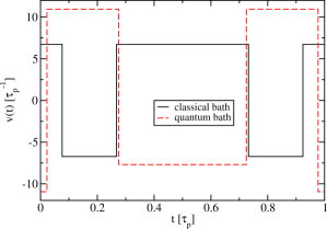
Figure 1: (Color online) Symmetric second order $\pi$ pulse with piecewise constant amplitude suppressing pure dephasing. The symmetric switching instants are $\tau_{1}=0.07623078\tau_{p}$, $\tau_{2}=0.26784319\tau_{p}$, $\tau_{3}=1-\tau_{2}$ and $\tau_{4}=1-\tau_{1}$, the amplitude is $\pm 6.72572865\tau_{p}^{-1}$

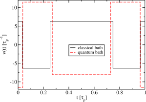
Figure 2: (Color online) Symmetric second order $\frac{\pi}{2}$ pulse with piecewise constant amplitude suppressing pure dephasing. The symmetric switching instants are $\tau_{1}=0.03312609\tau_{p}$, $\tau_{2}=0.25209296\tau_{p}$, $\tau_{3}=1-\tau_{2}$ and $\tau_{4}=1-\tau_{1}$, the amplitude is $\pm 6.32709469\tau_{p}^{-1}$.

Comparing the integral equations for the first and the second order with those derived for a quantum bath [29] we find that they are identical in first order. In second order, they are similar in form but in the quantum case there are three equations while two of them vanish in the classical case because the system Hamiltonian (20) commutes with itself at different times. This implies that it is less demanding to find a numerical solution for the equations (25) and (3) in the classical case than in the quantum case. Practically, pulses can be found with a lower amplitude than in the quantum case. In Figs. 1 and 2 examples of a $\pi$ and a $\pi/2$ second-order pulses with piecewise constant amplitudes are shown and compared to the corresponding pulses for a quantum bath [29]. Clearly, the maximal amplitudes of the classical pulses are lower. A technical remark is in order: Although the classical pulses have to fulfill less conditions we designed them with the same number of switching instants as the quantum pulses. But the absolute value of the amplitudes of the classical pulses is always the same while it varies in the quantum case. So the amplitude values are the additional variables needed in the quantum case.

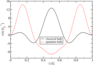
Figure 3: (Color online) Symmetric $\pi$ pulse with continuosly modulated amplitude correcting up to second order suppressing pure dephasing. The function $v(t)$ is parametrized by Eq. (3) with $a=-1.92179255$ and $b=2.86838351$.

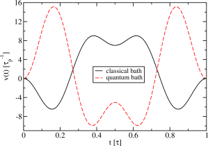
Figure 4: (Color online) Symmetric $\frac{\pi}{2}$ pulse with continuously modulated amplitude correcting up to second order suppressing pure dephasing. The function $v(t)$ is parametrized by Eq. (3) with $a=-5.41258549$ and $b=-3.48909926$.

Equations (25,3) can also be solved for continuous pulses. For symmetric pulses the function $v(t)$ can be represented by

$$v(t)= \frac{\theta}{2}+\left(a+\frac{\theta}{2}\right)\cos\left(\frac{2\pi}{\tau_{\text{p}}}t\right)+(b-a)\cos\left(\frac{4\pi}{\tau_{\text{p}}}t\right)$$

$$-b\cos\left(\frac{6\pi}{\tau_{\text{p}}}t\right)$$ (28)

where $\theta$ is either $\pi$ or $\pi/2$ and $a$ and $b$ are constants. The pulse fulfills the requirements $v(0)=v(\tau_{\text{p}})=0$ and $v^{\prime}(0)=v^{\prime}(\tau_{\text{p}})=0$, as shown in Figs. (3) and (4). Also in this case the maximal amplitude is lower than in the quantum case.

All solutions presented above were obtained numerically. The piecewise constant solutions for amplitude modulation were found using “fsolve()” from the “scipy” library for Python, which essentially is a wrapper around the “hybrd” and “hybrdj” algorithms from MINPACK. No further numerical calculations were needed to obtain those solutions because the integrations were done analytically. This was achieved by partitioning the integration domain into the intervals between the switching instants. In this way $\psi(t)$ becomes a linear function within each interval of the partition such that the contribution of each interval is analytically available.

To obtain continuous solutions for amplitude modulation, the GNU Scientific Library (GSL) was used for performance reasons. To find the multidimensional roots of the necessary sets of equations, the “gsl_multiroot_fsolver_hybrids” algorithm was used. It is very similar to the “hybrd” algorithm in MINPACK except for the internal scaling. A proposed solution is accepted if the residue, i.e., the sum over all absolute values $\sum_{i}\left|f_{i}\right|$, is less than $10^{-10}$. The integrand values $f_{i}$ themselves are calculated using “gsl_integration_gaq” which relies on an adaptive numerical integration using the $61$ point Gauss-Kronrod rules until the estimate of the absolute global error is less than $10^{-12}$. To compute multiple integrals, calls of “gsl_integration_gaq” were nested appropriately.

4 Frequency Modulated Pulses for Pure Dephasing

It is important to analyze the case of frequency modulated pulses as well because there may be experimental setups where frequency modulation (FM) can be implemented much easier or more accurately than amplitude modulation. There is only an initial and a final jump in the amplitude, the remaining control evolves smoothly. The initial and final transients will be discussed in the following section. Another advantage of frequency modulated pulses is that rotations about different axes can be realized in a natural way. Thereby, all kinds of deviations from the initial spin state can be compensated including spin relaxation. This latter point will be exploited in more detail in section 6.

We study pulses acting only in the $xy$-plane of the spin orientation with a fixed amplitude $V_{0}:=\left|\vec{v}\right|$. In the rotating frame taking the Larmor frequency $\omega_{\mathrm{L}}$ into account, the current axis of rotation is given by

$$\vec{v}(t)=\left(\begin{array}[]{c}V_{0}\cos(\Omega(t))\\ V_{0}\sin(\Omega(t))\\ 0\end{array}\right)$$ (32)

where $\Omega(t)$ is a time dependent phase which is tuned externally. The control Hamiltonian $H_{0}$ is realized by applying a field perpendicular to the $\sigma_{z}$-axis which is rotating with the Larmor frequency in the laboratory frame

$$H_{0}^{\text{lab}}=V_{0}\left[\sigma_{x}\cos(\omega_{\mathrm{L}}t-\Omega(t))-\sigma_{y}\sin(\omega_{\mathrm{L}}t-\Omega(t))\right].$$ (33)

The derivative $\partial_{t}\Omega(t)$ of the time dependent phase represents the deviation of the current frequency from the Larmor frequency. In this sense Eq. (33) describes a frequency modulated pulse. In the rotating frame we have

$$H_{0}(t)=\vec{v}(t)\cdot\vec{\sigma}.$$ (34)

In order to find $\hat{a}(t)$ and $\psi(t)$ appearing in the parametrization (8) of the pulse one has to solve the differential equation (9). Because $\hat{a}(t)$ is a unit vector, it can be parametrized by two angles $\phi(t)$ and $\theta(t)$

$$\hat{a}(t):=\left(\begin{array}[]{c}a_{x}(t)\\ a_{y}(t)\\ a_{z}(t)\end{array}\right)=\left(\begin{array}[]{c}\sin(\theta(t))\cos(\phi(t))\\ \sin(\theta(t))\sin(\phi(t))\\ \cos(\theta(t))\end{array}\right).$$ (41)

Solving Eq. (9) for the time derivatives of $\psi(t)$, $\phi(t)$, and $\theta(t)$ we finally find

$$\partial_{t}\psi =2V_{0}\sin\theta\left[\sin\Omega\sin\phi+\cos\Omega\cos\phi\right]$$ (42a)

$$\partial_{t}\phi =V_{0}\frac{\left[\cos\frac{\psi}{2}\sin(\Omega-\phi)-\sin\frac{\psi}{2}\cos\theta\cos(\Omega-\phi)\right]}{\sin\frac{\psi}{2}\sin\theta}$$ (42b)

$$\partial_{t}\theta =V_{0}\frac{\left[\cos\frac{\psi}{2}\cos\theta\cos(\Omega-\phi)+\sin\frac{\psi}{2}\sin(\Omega-\phi)\right]}{\sin\frac{\psi}{2}}.$$ (42c)

The seeming singularities for $\theta=m\pi,m\in\mathbb{Z}$ on the right hand sides of Eqs. (42b) and (42c) have no physical reason. They only result from the choice of spherical coordinates where $\phi$ is ill-defined for $\theta=m\pi,m\in\mathbb{Z}$. In contrast, the global axis of rotation $\hat{a}$ is ill-defined if $\psi$ is a multiple of $2\pi$ because then the unitary of the total pulse is plus or minus the identity so that $\hat{a}$ could take any direction. This is reflected in the singuarities of $\psi=2m\pi,m\in\mathbb{Z}$.

At $t=0$ the current axis of rotation $\vec{v}$ and the global one $\vec{a}$ coincide. The former lies by construction in the $xy$-plane implying the inital conditions

$$\underset{t\to 0}{\lim}\theta(t) =\frac{\pi}{2},$$ (43a)

$$\underset{t\to 0}{\lim}\psi(t) =0,$$ (43b)

$$\underset{t\to 0}{\lim}\phi(t) =\Omega(0).$$ (43c)

Note that the last two equations represent our arbitrary choice which direction is the $x$-direction for the spins and where the phase $\Omega$ starts. In the numerical solutions below we will use $\Omega(0)=0$. Inspecting the limit $t\to 0$ one additionally finds

$$\partial_{t}\phi\mid_{t=0} =\left.\frac{\partial_{t}\Omega(t)}{2}\right|_{t=0}$$ (44a)

$$\partial_{t}\theta\mid_{t=0} =0.$$ (44b)

The derivative $\partial_{t}\psi$ follows trivially from Eq. (42a).

We aim at solutions of Eqs. (15a) and (15b) both for $\pi$ and $\pi/2$ rotations and for pure dephasing $\vec{\eta}\left(t\right)=\left(0,0,\eta\left(t\right)\right)$. The corresponding vector $\vec{n}_{\vec{\eta}}(t)$ read

$$\vec{n}_{\vec{\eta}}(t)\equiv\eta\left(t\right)\begin{pmatrix}n_{x}\left(t\right)\\ n_{y}\left(t\right)\\ n_{z}\left(t\right)\end{pmatrix}$$

$$=\eta\left(t\right)\begin{pmatrix}-a_{y}\sin\left(\psi\right)+\left(1-\cos\left(\psi\right)\right)a_{x}a_{z}\\ a_{x}\sin\left(\psi\right)+\left(1-\cos\left(\psi\right)\right)a_{y}a_{z}\\ \cos\left(\psi\right)+\left(1-\cos\left(\psi\right)\right)a_{z}^{2}\end{pmatrix}.$$ (45)

For the sake of simplicity we have omitted the explicit time dependence of $a$ and $\psi$.

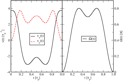
Figure 5: (Color online) First order $\pi$ pulse suppressing pure dephasing by frequency modulation. Parameters given in Tab. 1.

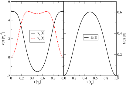
Figure 6: (Color online) First order $\pi/2$ pulse suppressing pure dephasing by frequency modulation. Parameters given in Tab. 1.

1st order FM $\pi$- and $\frac{\pi}{2}$ pulses
$\pi$-pulse		$\frac{\pi}{2}$-pulse
$V_{0}$	$3.751157$	$V_{0}$	$4.928277$
$b_{1}$	$0$	$b_{1}$	$0$
$b_{2}$	$-1.090479$	$b_{2}$	$-0.944852$
$b_{3}$	$0$	$b_{3}$	$0$
$b_{4}$	$-0.588913$	$b_{4}$	$-0.122088$

Table 1: Parameters for the first order frequency modulated (FM) pulses suppressing pure dephasing by satisfying Eqs. (50) for compensating a classical bath. The coefficients can be compared to those derived in Ref. [30] for a quantum bath. The dimensionless coefficients $b_{n}$ refer to the ansatz (46). The amplitudes $V_{0}$ are given in units of $1/\tau_{\mathrm{p}}$. The odd coefficients are numerically $0$ within $10^{-13}$.

For the phase $\Omega(t)$ we use the Fourier series ansatz

$$\Omega(t) ={\underset{n}{\sum}}b_{2n-1}\sin\big{(}\frac{2\pi nt}{\tau_{\text{ p}}}\big{)}+b_{2n}\big{[}\cos\big{(}\frac{2\pi nt}{\tau_{\text{ p}}}\big{)}-1\big{]}.$$ (46)

The value $\theta(\tau_{\mathrm{p}})$ is fixed by the fact, that the final axis of rotation has to be perpendicular to $\sigma_{z}$ to rotate the spin by the full angle $\psi(\tau_{\mathrm{p}})$. Thus one has

$$\theta(\tau_{\mathrm{p}})=\frac{\pi}{2}.$$ (47)

In first order, explicit computation yields

$$\tau_{\text{p}}\tilde{H}_{1}=\mu_{1,1}\sigma_{x}+\mu_{1,2}\sigma_{y}+\mu_{1,3}\sigma_{z}$$ (48)

with

$$\mu_{1,1} =\overline{\eta}_{z}\int\limits_{0}^{\tau_{\text{p}}}n_{xz}\left(t\right)\mathrm{dt}$$ (49a)

$$\mu_{1,2} =\overline{\eta}_{z}\int\limits_{0}^{\tau_{\text{p}}}n_{yz}\left(t\right)\mathrm{dt}$$ (49b)

$$\mu_{1,3} =\overline{\eta}_{z}\int\limits_{0}^{\tau_{\text{p}}}n_{zz}\left(t\right)\mathrm{dt},$$ (49c)

where the functions $n_{\alpha\beta}(t)$ with $\alpha,\beta\in\{x,y,z\}$ are given by the matrix elements of the rotation matrix $D_{\hat{a}}(-\psi)$ in (66) in B. Thus, for first order pulses one has to achieve

$$0=\mu_{1,i}$$ (50)

for $i\in\{1,2,3\}$. Typical solutions for $\pi$ and $\pi/2$ pulses are shown in Figs. 5 and 6. The parameters are given in Tab. 1.

In second order we similarly obtain

$$\tau_{\text{p}}\tilde{H}_{2}=\mu_{2,1}\sigma_{x}+\mu_{2,2}\sigma_{y}+\mu_{2,3}\sigma_{z}$$ (51)

with

$$\mu_{2,1}= \int\limits_{0}^{\tau_{\text{p}}}\int\limits_{0}^{t_{1}}(n_{yz,1}n_{zz,2}-n_{zz,1}n_{yz,2})\mathrm{dt_{2}}\mathrm{dt_{1}}$$ (52a)

$$\mu_{2,2}= \int\limits_{0}^{\tau_{\text{p}}}\int\limits_{0}^{t_{1}}(n_{zz,1}n_{xz,2}-n_{xz,1}n_{zz,2})\mathrm{dt_{2}}\mathrm{dt_{1}}$$ (52b)

$$\mu_{2,3}= \int\limits_{0}^{\tau_{\text{p}}}\int\limits_{0}^{t_{1}}(n_{xz,1}n_{yz,2}-n_{xz,1}n_{xz,2})\mathrm{dt_{2}}\mathrm{dt_{1}},$$ (52c)

using the shorthand $n_{\alpha\beta,k}:=n_{\alpha\beta}\left(t_{k}\right)$ where $k\in\{1,2\}$. Thus a second order FM pulse has to fulfill (50) and

$$0=\mu_{2,i}.$$ (53)

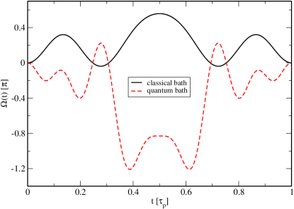
Figure 7: (Color online) Minimized second order FM $\pi$ pulse suppressing pure dephasing with $\Omega(t)$ as in Eq. (46). The coefficients for this pulse are given in Tab. 2.

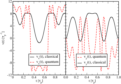
Figure 8: (Color online) Amplitudes for the same pulse as in Fig. 7.

Minimized 2nd order $\pi$ FM pulses
classical		quantum
$V_{0}$	$8.129097$	$V_{0}$	$10.707115$
$b_{1}$	$0$	$b_{1}$	$0$
$b_{2}$	$-0.381075$	$b_{2}$	$1.392956$
$b_{3}$	$0$	$b_{3}$	$0$
$b_{4}$	$0.450018$	$b_{4}$	$-0.705159$
$b_{5}$	$0$	$b_{5}$	$0$
$b_{6}$	$-0.496673$	$b_{6}$	$0.133042$
$b_{7}$	$0$	$b_{7}$	$0$
$b_{8}$	$-0.241963$	$b_{8}$	$0.690594$
		$b_{9}$	$0$
		$b_{10}$	$-0.695501$
		$b_{14}$	$0.472195$

Table 2: Parameters of the minimized FM $\pi$ pulses suppressing pure dephasing by satisfying the first and second order Eqs. (50) and (53) for a classical or the corresponding conditions for a quantum dephasing bath in Ref. [30]. The dimensionless coefficients $b_{n}$ refer to Eq. (46). The amplitudes $V_{0}$ are given in units of $1/\tau_{\mathrm{p}}$. The odd coefficients are numerically $0$ within $10^{-10}$.

Minimized 2nd order $\pi/2$ FM pulses
classic		quantum
$V_{0}$	7.405785	$V_{0}$	8.435414
$b_{1}$	1.524556	$b_{1}$	-1.820216
$b_{2}$	-0.349899	$b_{2}$	-0.351972
$b_{3}$	0.325909	$b_{3}$	0.030436
$b_{4}$	0.411212	$b_{4}$	0.521648
$b_{5}$	0.690512	$b_{5}$	-0.555341
$b_{6}$	-0.510771	$b_{6}$	-0.387557
$b_{7}$	0.347745	$b_{7}$	0.451462
$b_{11}$	0.019634	$b_{8}$	-0.193733
		$b_{9}$	-0.161450
		$b_{10}$	-0.282067
		$b_{14}$	0.047116

Table 3: Parameters of the minimized FM $\pi/2$ pulses suppressing pure dephasing by satisfying all first and second order Eqs. (50) and (53) for a classical bath or the corresponding conditions for a quantum bath in Ref. [30]. The dimensionless coefficients $b_{n}$ refer to Eq. (46). The amplitudes $V_{0}$ are given in units of $1/\tau_{\mathrm{p}}$.

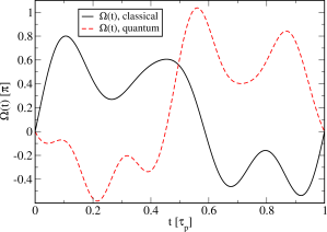
Figure 9: (Color online) Minimized second order FM $\pi/2$ pulse suppressing pure dephasing with $\Omega(t)$ as in Eq. (46). The coefficients for this pulse are given in Tab. 3.

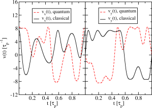
Figure 10: (Color online) Amplitudes for the same pulse as in Fig. 9.

Solutions for second order pulses with frequency modulation are shown in Figs. 7 and 8 for $\pi$ pulses and in Figs. 9 and 10 for $\pi/2$ pulse. In Figs. 7 and 9 the phases $\Omega(t)$ are shown while in Figs. 8 and 10 the corresponding amplitudes are plotted. These pulses are minimized in the following way. Since it is important to realize pulses with small amplitudes for practical purposes, we studied sets of Fourier coefficients in (46) with one coefficient more than necessary for the conditions (50) and (53). We used this freedom to minimize the amplitude and carried this out for four different choices of the Fourier coefficients. The solution with the minimal amplitude out of the four minima is shown. The characteristics of the pulses are reported in Tabs. 2 and 3, respectively. We stress again that the classical case requires less coefficients than the quantum case. The maximal amplitudes of the classical pulses are smaller than the amplitudes for the quantum pulse, as can be seen comparing the values in the tables or the plots for $v_{x}$ and $v_{y}$. Moreover, the pulses suppressing classical noise have a simpler form.

Obviously, the solutions are symmetric because all sine coefficients in Tab. 2 vanish to numerical accuracy. This holds for the classical as well as for the quantum case. Deviations from this symmetric shape in the results of Ref. [30] are due to the lower precision of the numerics used in this preceding article.

In addition to the tools employed already for AM pulses, finding frequency modulated pulses requires to solve a system of three coupled ordinary differential equations in each step of the multidimensional root search. This was done by using “gsl_odeiv2_system” with a stepping of the type “gsl_odeiv2_step_rk4”. Thus a fourth order Runge-Kutta integration with adaptive step size governed by the double step method to keep the local absolute error estimate in the order of magnitude of $10^{-15}$.

5 Amplitude and Frequency Modulated Pulses

Allowing for the modulation of amplitude and frequency leads to a humongous parameter space. Thus we restrict ourselves to illustrating that the frequency modulated pulses of the previous section can be modified to account for smooth transients when the pulses are switched on and off. Such transients are generic in experimental realizations.

To describe the transient region we define

$$f(t):=\left\{\begin{array}[]{rr}f_{\text{on}}(t)&\mbox{ $0\leq t<\tau_{\text{s}}$}\\ 1&\mbox{ $\tau_{\text{s}}\leq t<\tau_{\text{p}}-\tau_{\text{s}}$}\\ 1-f_{\text{on}}[t-(1-\tau_{\text{s}})]&\mbox{ $\tau_{\text{p}}-\tau_{\text{s}}\leq t\leq\tau_{\text{p}}$}\end{array}\right.$$ (57)

where $f_{\text{on}}(t):=\sin^{2}\left(\pi t/2\tau_{\text{s}}\right)$. The actual amplitude $V(t)$ is given by $V_{0}f(t)$. Then $\tau_{\text{s}}$ stands for the time needed to reach the amplitude $V_{0}$ from zero amplitude or vice-versa, see Fig. 11.

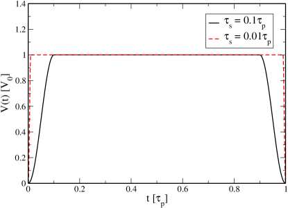
Figure 11: (Color online) A more realistic variation of the amplitude $V(t)=V_{0}f(t)$ according to Eq. (57) for frequency modulated pulses. Note the transients for switching the pulse on and off.

In this section, we report the results for $\tau_{\text{s}}=0.1\tau_{\text{p}}$. In A, results for other values of $\tau_{\text{s}}$ are included for comparison. The parametrization of $\Omega(t)$ and ${\hat{a}}(t)$ are the same as in section 4.

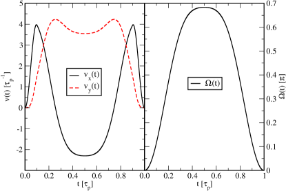
Figure 12: (Color online) AM+FM first order $\pi$ pulse suppressing pure dephasing for $\tau_{\text{s}}=0.1\tau_{\text{p}}$. The phase $\Omega(t)$ is parametrized as in Eq. (46). The coefficients of this pulse are given in Tab. 4.

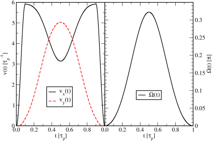
Figure 13: (Color online) AM+FM first order $\pi/2$ pulse suppressing pure dephasing for $\tau_{\text{s}}=0.1\tau_{\text{p}}$. The phase $\Omega(t)$ is parametrized as in Eq. (46). The coefficients of this pulse are given in Tab. 4.

First order $\pi$ and $\pi/2$ AM+FM pulses
$\pi$		$\pi/2$
$V_{0}$	4.232216	$V_{0}$	5.930552
$b_{1}$	$0$	$b_{1}$	$0$
$b_{2}$	-1.073059	$b_{2}$	-0.506131
$b_{3}$	$0$	$b_{3}$	$0$
$b_{4}$	-0.233720	$b_{4}$	0.053241

Table 4: Parameters for the $\pi$ and $\pi/2$ AM+FM pulses suppressing pure dephasing with $\tau_{\text{s}}=0.1\tau_{\text{p}}$. The coefficients $b_{n}$ refer to Eq. (46). The amplitudes $V_{0}$ are given in units of $1/\tau_{\mathrm{p}}$. The odd coefficients vanish numerically with in $10^{-11}$.

Examples for first order AM+FM $\pi$ and $\pi/2$ pulses are plotted in Figs. 12 and 13 and the coefficients of the parametrization can be found in Tab. 4. The maximum amplitude of the AM+FM pulses is lower than the amplitude of the continuous AM pulses and of the FM pulses derived for a quantum bath [29]. It is comparable to the amplitude of the well-known SCORPSE $\pi$ pulses [35, 36] which is $7\pi/6\approx 3.7$ in units of $\tau_{\text{p}}^{-1}$. In comparison to the pure FM pulses of first order shown in Figs. 5 and 6 with parameters given in Tab. 1 we clearly see that a bit larger amplitudes are required for finite transients as was to be expected.

2nd order AM+FM $\pi$ and $\pi/2$ pulses
$\pi$		$\pi/2$
$V_{0}$	9.076304	$V_{0}$	10.450781
$b_{1}$	$0$	$b_{1}$	$0$
$b_{2}$	-0.436689	$b_{2}$	-0.123441
$b_{3}$	$0$	$b_{3}$	$0$
$b_{4}$	0.305937	$b_{4}$	-0.130381
$b_{5}$	$0$	$b_{5}$	$0$
$b_{6}$	-0.585209	$b_{6}$	-0.679511
$b_{7}$	$0$	$b_{7}$	$0$

Table 5: Parameters for the $\pi$ and $\pi/2$ AM+FM pulses suppressing pure dephasing by satisfying the first and second order Eqs. (50) and (53) for a classical bath. The coefficients $b_{n}$ refer to Eq.  (46). The amplitudes $V_{0}$ are given in units of $1/\tau_{\mathrm{p}}$. The odd coefficients vanish numerically within $10^{-9}$.

Analogous considerations hold for second order pulses. They are plotted in Figs. 14 and 15. Their coefficients are listed in Tab. 5.

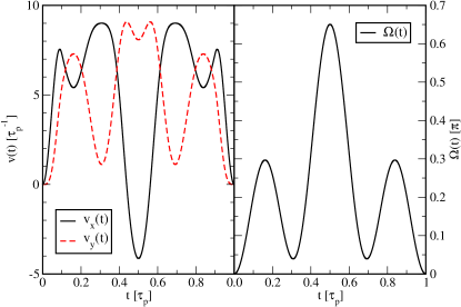
Figure 14: (Color online) Minimized second order AM+FM $\pi$ pulse suppressing pure dephasing with $\Omega(t)$ as in Eq. (46). The coefficients are given in Tab. 5.

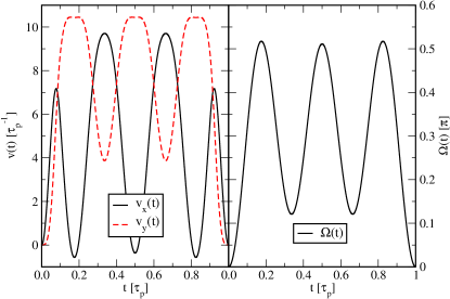
Figure 15: (Color online) Minimized second order AM+FM $\pi/2$ pulse suppressing pure dephasing with $\Omega(t)$ as in Eq. (46). The coefficients are given in Tab. 5.

6 Frequency Modulated Pulses for General Decoherence

In section 4 on frequency modulated pulses we pointed out that one of their major assets is that they realize rotations about two independent spin axes. Hence FM pulses may correct not only dephasing without spin flips but also longitudinal relaxation including spin flips. We treat this situation here. Thus we deal with the Hamiltonian in (5) where all three components $\eta_{\alpha}$ ($\alpha\in\{x,y,z\}$) of $\vec{\eta}$ are present.

We consider a bath with cylindrical symmetry generic for an NMR experiment where the $z$-axis of the spin is distinguished by a large magnetic field and the system is rotationally invariant around this axis. Considering rotations by $\pi$ and $\frac{\pi}{2}$ about $\sigma_{z}$ one easily finds that the averages of $\vec{\eta}$ fulfill

$$\overline{\eta}_{x}=\overline{\eta}_{y} =0$$ (58)

Additionally, second order pulse require the autocorrelation

$$g_{\alpha\alpha}\left(t=0\right)=\overline{\eta}_{\alpha}^{2}+s^{2}_{\alpha}+{\cal O}(t).$$ (59)

with $\alpha\in\{x,y,z\}$. We do not mention terms linear in $|t|$ because we aim at second order pulses at most. In principle, the cross correlations $g_{\alpha\neq\beta}(t=0)$ may also matter. But the cylindrical symmetry in combination with the antisymmetry of $g_{xy}(-t)=-g_{xy}(t)$ imply that all cross correlations $g_{\alpha\neq\beta}(t=0)$ vanish. In addition, $s_{x}^{2}=g_{xx}(0)=g_{yy}(0)$ is implied.

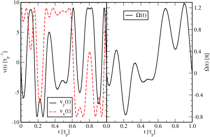
Figure 16: (Color online) Minimized second order FM $\pi$ pulse suppressing general decoherence with $\Omega(t)$ as in Eq. (46). The coefficients are given in Tab. 6.

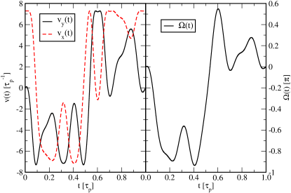
Figure 17: (Color online) Minimized second order FM $\pi/2$ pulse suppressing general decoherence with $\Omega(t)$ as in Eq. (46). The coefficients are given in Tab. 6.

On the basis of the expectation values (6), the vanishing of the first term, see Eq. (48), requires the vanishing of the same integral equations as in the case of pure dephasing (49) for frequency modulated pulses. Hence the same solutions result presented in the two previous sections.

In second order, we use the variances and vanishing cross correlations to conclude that the vanishing of

$$\tau_{\text{p}}\tilde{H}_{2}=(\mu_{2,1}+\mu_{2,4})\sigma_{x}+(\mu_{2,2}+\mu_{2,5})\sigma_{y}+(\mu_{2,3}+\mu_{2,6})\sigma_{z}$$ (60)

requires the coefficients $\mu_{2,i}$ to take the value zero

$$\mu_{2,1} =s^{2}_{x}\int\limits_{0}^{\tau_{p}}\int\limits_{0}^{t_{1}}[n_{yx,1}n_{zx,2}+n_{yy,1}n_{zy,2}$$

$$-\left(n_{zx,1}n_{yx,2}+n_{zy,1}n_{yy,2}\right)]\mathrm{dt_{2}}\mathrm{dt_{1}}$$ (61a)

$$\mu_{2,2} =s^{2}_{x}\int\limits_{0}^{\tau_{p}}\int\limits_{0}^{t_{1}}[n_{zx,1}n_{xx,2}+n_{zy,1}n_{xy,2}$$

$$-\left(n_{xx,1}n_{zx,2}+n_{xy,1}n_{zy,2}\right)]\mathrm{dt_{2}}\mathrm{dt_{1}}$$ (61b)

$$\mu_{2,3} =s^{2}_{x}\int\limits_{0}^{\tau_{p}}\int\limits_{0}^{t_{1}}[n_{xx,1}n_{yx,2}+n_{xy,1}n_{yy,2}$$

$$-\left(n_{yx,1}n_{xx,2}+n_{yy,1}n_{xy,2}\right)]\mathrm{dt_{2}}\mathrm{dt_{1}}$$ (61c)

$$\mu_{2,4} =\left(\overline{\eta}_{z}^{2}+s^{2}_{z}\right)\int\limits_{0}^{\tau_{p}}\int\limits_{0}^{t_{1}}[n_{yz}\left(t_{1}\right)n_{zz}\left(t_{2}\right)$$

$$\quad-n_{zz}\left(t_{1}\right)n_{yz}\left(t_{2}\right)]\mathrm{dt_{2}}\mathrm{dt_{1}}$$ (61d)

$$\mu_{2,5} =\left(\overline{\eta}_{z}^{2}+s^{2}_{z}\right)\int\limits_{0}^{\tau_{p}}\int\limits_{0}^{t_{1}}[n_{zz}\left(t_{1}\right)n_{xz}\left(t_{2}\right)$$

$$\quad-n_{xz}\left(t_{1}\right)n_{zz}\left(t_{2}\right)]\mathrm{dt_{2}}\mathrm{dt_{1}}$$ (61e)

$$\mu_{2,6} =\left(\overline{\eta}_{z}^{2}+s^{2}_{z}\right)\int\limits_{0}^{\tau_{p}}\int\limits_{0}^{t_{1}}[n_{xz}\left(t_{1}\right)n_{yz}\left(t_{2}\right)$$

$$\quad-n_{yz}\left(t_{1}\right)n_{xz}\left(t_{2}\right)]\mathrm{dt_{2}}\mathrm{dt_{1}}.$$ (61f)

Note that we have to require that each $\mu_{2,i}$ vanishes even though they appear in pairs in front of the Pauli matrices in (60) because we do not want to make assumptions of the relative size of $s_{x}^{2}$ and $\overline{\eta}_{z}^{2}+s^{2}_{z}$.

The parametrization of $\Omega(t)$ and ${\hat{a}}(t)$ are chosen as before in sections 4 and 5. Solutions to the conditions $\mu_{1,i}=0$ and $\mu_{2,i}=0$ are shown in Fig. 16 for a $\pi$ pulse and in Fig. 17 for a $\pi/2$ pulse. The parameters of these pulses are reported in Tab. 6. The amplitudes of these pulses have been minimized as described before.

Comparing the amplitudes in Tab. 6 with those for classical pulses in Tabs. 2 and 3, it is clear that the suppression of general decoherence requires higher amplitudes or longer pulses, respectively. But the increase in amplitude is not very large. For the $\pi$ pulse, the amplitude is increased by 12% and for the $\pi/2$ pulse it is even lowered by 1%. This finding appears contradictory at first sight because more conditions have to be fulfilled for general decoherence. The contradiction is resolved by the observation that we consider more coefficients in the construction of the pulse suppressing general decoherence than we do in the construction of the pulse suppressing pure dephasing, see Tabs. 3 and 6. Of course, the $\pi/2$ pulse suppressing general decoherence fulfills also the conditions for the suppression of pure dephasing. It is remarkable that the additional conditions for general decoherence can be fulfilled at only moderate additional effort. Hence one may realize a pulse which not only suppresses transversal decoherence but also longitudinal decoherence.

Another intriguing possibility is to use the pulses found as replacement for XY4 and XY8 cycles [6, 7]. The main difference between the net effect of XY4 to the $\pi$ pulse suppressing general decoherence in Fig. 16 and Tab. 6 is that XY4 is designed to be a no-operation (NOOP) sequence while the $\pi$ pulse realizes a spin flip. But if the $\pi$ pulses is applied a second time in time-reversed order $\Omega(\tau)\to\Omega(\tau_{\text{p}}-\tau)$ it realizes again a second order $\pi$ pulses. Thus the effect of both pulses back-to-back is a $2\pi$ pulse which reduces to a mere phase factor $-1$ without effect on the actual spin state. Hence, such a composite pulse of length $2\tau_{\text{p}}$

$$\pi\Big{|}_{\text{FM,forward}}-\pi\Big{|}_{\text{FM,backward}}$$ (62)

is symmetric and corresponds to an XY8 cycle in the sense that it suppresses spin dephasing and spin flips; thus it suppresses general decoherence up to second order. The intriguing aspect is that this composite pulse is an always-on pulse and does not consist of 8 individual pulses. Thus its amplitude is much lower than the amplitude needed in an XY8 cycle. For given pulse length one can reduce the total energy $\propto V_{0}^{2}\tau_{\text{p}}$ needed for the coherent control. For given maximal amplitude the cycle can be performed much more rapidly. This opens a promising route to more effective control calling for experimental verification.

2nd order FM $\pi$ and $\pi/2$ pulses for general decoherence
$\pi$		$\pi/2$
$V_{0}$	$9.079728$	$V_{0}$	$7.297361$
$b_{1}$	$1.818085$	$b_{1}$	$-1.793195$
$b_{2}$	$0.514273$	$b_{2}$	$0.223583$
$b_{3}$	$-0.231238$	$b_{3}$	$0.221590$
$b_{4}$	$-0.220323$	$b_{4}$	$0.324311$
$b_{5}$	$0.014857$	$b_{5}$	$-0.579783$
$b_{6}$	$0.508720$	$b_{6}$	$0.272144$
$b_{7}$	$-0.439837$	$b_{7}$	$0.507358$
$b_{8}$	$-0.816150$	$b_{8}$	$-0.119786$
$b_{9}$	$-0.332547$	$b_{9}$	$-0.011429$
$b_{10}$	$-0.846412$	$b_{10}$	$0.069581$
$b_{11}$	$-0.249481$	$b_{13}$	$0.219071$

Table 6: Parameters for the minimized FM $\pi$ and $\pi/2$ pulses suppressing general decoherence. The coefficients $b_{n}$ refer to Eq. (46). The amplitudes $V_{0}$ are given in units of $1/\tau_{\mathrm{p}}$.

7 Conclusions

Coherent control of quantum systems is a very active field of current research. The simplest quantum system to be controlled generally is a two-level system which can be seen as a spin $S=1/2$. In particular, the coherent control of such spins is at the very heart of magnetic resonance techniques, where nuclear spins are manipulated, and of quantum information processing, where quantum bits are manipulated. Previously, pulses were designed to suppress the influence of a noisy quantum environment. Although this is the most general case it is cumbersome because many conditions have to be fulfilled and thus the necessary pulses are fairly complicated. They need relatively large amplitudes or they are relatively long. Both properties limit their practical relevance.

In practice, however, very often the environmental noise is dominated by classical fluctuations, for instance because it results from macroscopic degrees of freedom at relatively high temperature (room temperature). This led us to study pulses which suppress classical noise. Such pulses are subject to less conditions so that they can be simpler and of lower amplitudes or their duration $\tau_{\text{p}}$ can be shorter. We studied such pulses analytically by a systematic expansion in $\tau_{\text{p}}$. Pulses with amplitude modulation, which rotate the spin about a single fixed axis, and pulses with frequency modulation, which rotate the spin about a continuously varying axis in the $xy$-plane of the spin directions, are considered.

A purely dephasing bath is relevant if the energy splitting between the two levels is so large that the rotating frame approximation is applicable. Experimentally, the dephasing dominates if $T_{2}$ is much smaller than $T_{1}$. For this situation we presented first and second order pulses based on amplitude or on frequency modulation, respectively. We explicitly presented pulse shapes for $\pi$ and $\pi/2$ pulses which either flip the spin between up and down or which rotate them by 90^∘ from the $z$-axis. In all pulses suppressing classical noise we confirmed that their amplitudes are lower than for their previously known quantum counterparts. The only exception are first order pulses. In this order the quantum character is not manifest in the conditions so that they are identical for classical and for quantum baths.

Furthermore, we showed that combinations of amplitude and frequency modulation can also be treated. In particular, finite transients in the switching processes of amplitudes can be accounted for. Thus imperfections in the switching can be considered and they do not pose a conceptual problem.

Intriguingly, we could furthermore establish the existence of pulses which suppress classical general decoherence. This means that not only transversal dephasing but also longitudinal spin relaxation relying on spin flips can be suppressed. Amplitude modulation is not sufficient to this end because one needs at least two independent axes of rotation to suppress all kinds of spin errors. But frequency modulated pulses can do the job.

We found that the necessary amplitudes are at worst only moderately larger than for the suppression of pure dephasing alone. Thereby, we propose a single shaped pulse which has similar properties as cycles of pulses. In particular, a composite pulse of two $\pi$ pulses, which suppress general decoherence, can replace the well-known XY8 cycle. The asset of the composite pulse we are advocating here is that it is an always-on pulse. Hence the required amplitudes are much lower than those required for a cycle of very short pulses.

Of course, further research is called for. On the experimental side, studies of the performance of the proposed pulses are called for. A key question is whether the proposed shapes can be realized reliably enough to reach the predicted suppression of the noisy baths.

Theoretically, the question of the robustness of the proposed pulses towards imperfections in their realizations deserves investigations. For instance, simulations of the pulses in various baths are called for to guide experiment. In parallel, we believe that the necessary amplitudes can still be reduced by further minimization.

Finally, we point out that analogous expansions for coupled two-level systems have hardly attracted attention so far in spite of their relevance of two-qubit gates in quantum information processing.

8 Acknowledgements

We acknowledge financial support of the DFG in Project UH 90/5-1.

Appendix A Pulses with Amplitude and Frequency Modulation

In section 5, we showed an example of two FM pulses with angle $\pi$ and $\pi/2$ and finite transients of amplitude for switching on and off. Each transient takes a fraction $\tau_{\text{s}}/\tau_{\text{p}}$ of the total time $\tau_{\text{p}}$ of the pulse. Here we provide further $\pi$ pulses with shorter transient time in Tab.  7 in first order and in Tab.  8 in second order. The parameters for the first order pulses are to be compared to those reported in Tab. 4. Remarkably, the amplitude does not increase monotonically on increasing $\tau_{\text{s}}/\tau_{\text{p}}$ in Tab. 7.

The second order parameters illustrate that amplitude and frequency modulation can also be combined in second order. The parameters can be compared to those of pure FM pulses given in Tab. 2.

1st order AM+FM $\pi$pulses
$\tau_{\text{s}}=0.01\tau_{\text{p}}$		$\tau_{\text{s}}=0.001\tau_{\text{p}}$
$V_{0}$	$3.907279$	$V_{0}$	$4.016102$
$b_{1}$	$0$	$b_{1}$	$0$
$b_{2}$	$-0.892324$	$b_{2}$	$-0.791296$
$b_{3}$	$0$	$b_{3}$	$0$
$b_{4}$	$-0.196455$	$b_{4}$	$-0.040110$

Table 7: Parameters of AM+FM first order $\pi$ suppressing pure dephasing for two switching times $\tau_{\text{s}}$. The dimensionless coefficients $b_{n}$ refer to Eq. (46). The amplitudes $V_{0}$ are given in units of $1/\tau_{\mathrm{p}}$. The odd coefficients vanish within $10^{-11}$.

2nd order AM+FM $\pi$pulses
$\tau_{\text{s}}=0.1\tau_{\text{p}}$		$\tau_{\text{s}}=0.01\tau_{\text{p}}$
$V_{0}$	$9.076304$	$V_{0}$	$8.486171$
$b_{2}$	$-0.436689$	$b_{2}$	$-0.309163$
$b_{4}$	$0.305937$	$b_{4}$	$0.507966$
$b_{6}$	$-0.585209$	$b_{6}$	$-0.437161$

Table 8: Parameters of AM+FM second order $\pi$ suppressing pure dephasing for two switching times $\tau_{\text{s}}$. The dimensionless coefficients $b_{n}$ refer to Eq. (46). The amplitudes $V_{0}$ are given in units of $1/\tau_{\mathrm{p}}$. The odd coefficients vanish within $10^{-9}$.

Appendix B Rotation Matrix

For the derivation of the matrix $D_{\hat{a}}(-\psi)$ we refer the reader to Ref. [29]. We obtain the matrix (66) below, where the time dependencies of $\psi(t)$ and $\hat{a}(t)$ are omitted for clarity. The matrix elements $[D_{\hat{a}}(-\psi)]_{\alpha\beta}$ define the quantities $n_{\alpha\beta}$ where we identify $x$ with $1$, $y$ with $2$, and $z$ with $3$.

$$D_{\hat{a}}(-\psi)=\left(\begin{array}[]{ccc}\cos\psi+(1-\cos\psi)a^{2}_{x}&a_{z}\sin\psi+(1-\cos\psi)a_{x}a_{y}&-a_{y}\sin\psi+(1-\cos\psi)a_{x}a_{z}\\ -a_{z}\sin\psi+(1-\cos\psi)a_{x}a_{y}&\cos\psi+(1-\cos\psi)a^{2}_{y}&a_{x}\sin\psi+(1-\cos\psi)a_{y}a_{z}\\ a_{y}\sin\psi+(1-\cos\psi)a_{x}a_{z}&-a_{x}\sin\psi+(1-\cos\psi)a_{y}a_{z}&\cos\psi+(1-\cos\psi)a^{2}_{z}\end{array}\right)$$ (66)

References

- [1] E. L. Hahn, Spin echoes, Phys. Rev. 80 (1950) 580.
- [2] H. Y. Carr, E. M. Purcell, Effects of diffusion on free precession in nuclear magnetic resonance experiments, Phys. Rev. 94 (1954) 630.
- [3] S. Meiboom, D. Gill, Modified spin-echo method for measuring nuclear relaxation times, Rev. Sci. Inst. 29 (1958) 688.
- [4] U. Haeberlen, High Resolution NMR in Solids: Selective Averaging, Academic Press, New York, 1976.
- [5] M. H. Levitt, Spin Dynamics, Wiley, Chichester, 2001.
- [6] A. A. Maudsley, Modified Carr-Purcell-Meiboom-Gill sequence for NMR Fourier imaging applications, J. Mag. Res. 69 (1986) 488.
- [7] T. Gullion, D. B. Baker, M. S. Conradi, New, compensated Carr-Purcell sequences, J. Mag. Res. 89 (1990) 479.
- [8] L. Viola, S. Lloyd, Dynamical suppression of decoherence in two-state quantum systems, Phys. Rev. A 58 (1998) 2733.
- [9] M. Ban, Photon-echo technique for reducing the decoherence of a quantum bit, J. Mod. Opt. 45 (1998) 2315.
- [10] L. Viola, E. Knill, S. Lloyd, Dynamical decoupling of open quantum systems, Phys. Rev. Lett. 82 (1999) 2417.
- [11] K. Khodjasteh, D. A. Lidar, Performance of deterministic dynamical decoupling schemes: Concatenated and periodic pulse sequences, Phys. Rev. A 75 (2007) 062310.
- [12] G. S. Uhrig, Keeping a quantum bit alive by optimized -pulse sequences, Phys. Rev. Lett. 98 (2007) 100504.
- [13] G. S. Uhrig, Erratum: Keeping a quantum bit alive by optimized -pulse sequences, Phys. Rev. Lett. 106 (2011) 129901.
- [14] G. S. Uhrig, Exact results on dynamical decoupling by -pulses in quantum information processes, New J. Phys. 10 (2008) 083024.
- [15] W. Yang, R.-B. Liu, Universality of uhrig dynamical decoupling for suppressing qubit pure dephasing and relaxation, Phys. Rev. Lett. 101 (2008) 180403.
- [16] L. Cywiński, R. M. Lutchyn, C. P. Nave, S. Das Sarma, How to enhance dephasing time in superconducting qubits, Phys. Rev. B 77 (2008) 174509.
- [17] S. Pasini, G. S. Uhrig, Optimized dynamical decoupling for power-law noise, Phys. Rev. A 81 (2010) 012309.
- [18] J. R. West, B. H. Fong, D. A. Lidar, Near-optimal dynamical decoupling of a qubit, Phys. Rev. Lett. 104 (2010) 130501.
- [19] S. Pasini, G. S. Uhrig, Optimized dynamical decoupling for time-dependent Hamiltonians, J. Phys. A: Math. Theo. 43 (2010) 132001.
- [20] G. Quiroz, D. A. Lidar, Quadratic dynamical decoupling with non-uniform error suppression, Phys. Rev. A 84 (2011) 042328.
- [21] W.-J-Kuo, D. A. Lidar, Quadratic dynamical decoupling: Universality proof and error analysis, Phys. Rev. A 84 (2011) 042329.
- [22] Z.-Y. Wang, R.-B. Liu, Protection of quantum systems by nested dynamical decoupling, Phys. Rev. A 83 (2011) 022306.
- [23] M. J. Biercuk, H. Uys, A. P. VanDevender, N. Shiga, W. M. Itano, J. J. Bollinger, Optimized dynamical decoupling in a model quantum memory, Nature 458 (2009) 996.
- [24] J. Du, X. Rong, N. Zhao, Y. Wang, J. Yang, R. B. Liu, Preserving electron spin coherence in solids by optimal dynamical decoupling, Nature 461 (2009) 1265.
- [25] G. Gordon, G. Kurizki, D. A. Lidar, Optimal dynamical decoherence control of a qubit, Phys. Rev. Lett. 101 (2008) 010403.
- [26] S. Pasini, T. Fischer, P. Karbach, G. S. Uhrig, Optimization of short coherent control pulses, Phys. Rev. A 77 (2008) 032315.
- [27] S. Pasini, G. S. Uhrig, Generalization of short coherent control pulses extension to arbitrary rotations, J. Phys. A: Math. Theo. 41 (2008) 312005.
- [28] K. Khodjasteh, D. A. Lidar, L. Viola, Arbitrarily accurate dynamical control in open quantum systems, Phys. Rev. Lett. 104 (2010) 090501.
- [29] S. Pasini, P. Karbach, C. Raas, G. S. Uhrig, Optimized pulses for the perturbative decoupling of spin and decoherence bath, Phys. Rev. A 80 (2009) 022328.
- [30] B. Fauseweh, S. Pasini, G. S. Uhrig, Frequency-modulated pulses for quantum bits coupled to time-dependent baths, Phys. Rev. A 85 (2012) 022310.
- [31] G. S. Uhrig, S. Pasini, Efficient coherent control by optimized sequences of pulses of finite duration, New J. Phys. 12 (2010) 045001.
- [32] S. Pasini, P. Karbach, G. S. Uhrig, High order coherent control sequences of finite-width pulses, Europhys. Lett. 96 (2011) 10003.
- [33] R. Tycko, Broadband population inversion, Phys. Rev. Lett. 51 (1983) 775.
- [34] M. H. Levitt, Composite pulses, Prog. NMR Spect. 18 (1986) 61.
- [35] H. K. Cummins, J. A. Jones, Use of composite rotations to correct systematic errors in NMR quantum computation, New J. Phys. 2 (2000) 6.
- [36] H. K. Cummins, G. Llewellyn, J. A. Jones, Tackling systematic errors in quantum logic gates with composite rotations, Phys. Rev. A 67 (2003) 042308.
- [37] T. E. Skinner, T. O. Reiss, B. Luy, N. Khaneja, S. J. Glaser, Application of optimal control theory to the design of broadband excitation pulses for high-resolution NMR, J. Mag. Res. 163 (2003) 8.
- [38] K. Kobzar, T. E. Skinner, N. Khanejac, S. J. Glaser, B. Luy, Exploring the limits of broadband excitation and inversion pulses, J. Mag. Res. 170 (2004) 236.
- [39] P. Sengupta, L. P. Pryadko, Scalable design of tailored soft pulses for coherent control, Phys. Rev. Lett. 95 (2005) 037202.
- [40] M. Möttönen, R. de Sousa, J. Zhang, K. B. Whaley, High-fidelity one-qubit operations under random telegraph noise, Phys. Rev. A 73 (2006) 022332.
- [41] W. G. Alway, J. A. Jones, Arbitrary precision composite pulses for NMR quantum computing, J. Magn. Res. 189 (2007) 114.
- [42] L. P. Pryadko, G. Quiroz, Soft-pulse dynamical decoupling in a cavity, Phys. Rev. A 77 (2008) 012330.
- [43] L. P. Pryadko, P. Sengupta, Second-order shaped pulses for solid-state quantum computation, Phys. Rev. A 78 (2008) 032336.
- [44] M. H. Levitt, Spin Dynamics, Basics of Nuclear Magnetic Resonance, John Wiley & Sons, Ltd, Chichester, 2005.
- [45] M. J. Biercuk, H. Bluhm, Phenomenological study of decoherence in solid-state spin qubits due to nuclear spin diffusion, Phys. Rev. B 83 (2011) 235316.
- [46] W. Magnus, On the exponential solution of differential equations for a linear operator, Comm. Pure Appl. Math. 7 (1954) 649.
- [47] S. Blanes, F. Casas, J. A. Oteo, J. Ros, The Magnus expansion and some of its applications, Phys. Rep. 470 (2009) 151.
- [48] G. de Lange, Z. H. Wang, D. Ristè, V. V. Dobrovitski, R. Hanson, Universal dynamical decoupling of a single solid-state spin from a spin bath, Science 30 (2010) 60.
- [49] G. C. Wick, The evaluation of the collision matrix, Phys. Rev. 80 (1950) 268.
- [50] L. M. K. Vandersypen, I. L. Chuang, NMR techniques for quantum control and computation, Rev. Mod. Phys. 76 (2004) 1037.