Two possible circumbinary planets in the eclipsing post-common envelope system NSVS 14256825

Abstract

We present an analysis of eclipse timings of the post-common envelope binary NSVS 14256825, which is composed of an sdOB star and a dM star in a close orbit ($P_{\rm orb}=0.110374$ days). High-speed photometry of this system was performed between July, 2010 and August, 2012. Ten new mid-eclipse times were analyzed together with all available eclipse times in the literature. We revisited the (O$-$C) diagram using a linear ephemeris and verified a clear orbital period variation. On the assumption that these orbital period variations are caused by light travel time effects, the (O$-$C) diagram can be explained by the presence of two circumbinary bodies, even though this explanation requires a longer baseline of observations to be fully tested. The orbital periods of the best solution would be $P_{c}\sim 3.5$ years and $P_{d}\sim 6.9$ years. The corresponding projected semi-major axes would be $a_{c}\sin i_{c}\sim 1.9$ AU and $a_{d}\sin i_{d}\sim 2.9$ AU. The masses of the external bodies would be $M_{c}\sim 2.9~{}M_{\rm Jupiter}$ and $M_{d}\sim 8.1~{}M_{\rm Jupiter}$, if we assume their orbits are coplanar with the close binary. Therefore NSVS 14256825 might be composed of a close binary with two circumbinary planets, though the orbital period variations is still open to other interpretations.

1 INTRODUCTION

Planetary formation and evolution around binary systems have become important topics since the discovery of the first exoplanet around the binary pulsar PSR B1620-26 (Backer et al., 1993). Theoretical studies have indicated that circumbinary planets can be formed and survive for a long time (Moriwaki & Nakagawa, 2004; Quintana & Lissauer, 2006). Characterization of such planets in different evolutionary stages of the host binary is crucial to constrain and test the formation and evolution models.

The common envelope (CE) phase in binary systems is dramatic for the planets survival. For a single star, Villaver & Livio (2007) have pointed out that planets more massive than two Jupiter masses around a main sequence star of 1 $M_{\odot}$ survive the planetary nebula stage down to orbital distances of 3 AU. The CE phase in binary systems is more complex than the nebular stage in single stars and its interaction with existing planets is still an open topic. Besides, a second generation of planets can be formed from a disk originated by the ejected envelope (van Winckel et al., 2009; Perets, 2011). Investigation of circumbinary planets in post-CE phase systems is fundamental to constrain observationally the minimum host binary-planet separation and to distinguish between planetary formation before and after the CE phase.

To date, circumbinary planets have been discovered in seven eclipsing post-CE binaries. All those discoveries were made using the eclipse timing variation technique. The main features of these planets are summarized in Table 1, which also shows the results for NSVS 14256825 presented in this paper.

NSVS 14256825 (hereafter referred to as NSVS 1425) is an eclipsing post-CE binary and consists of an sdOB star plus a dM star with an orbital period of 0.110374 days (Almeida et al., 2012). It was discovered using the Northern Sky Variability Survey (Woźniak et al., 2004). Kilkenny & Koen (2012) showed that the orbital period in NSVS 1425 is increasing at a rate of $\sim$ $1.1\times 10^{-10}~{}\rm s\,\,\rm s^{-1}$. Beuermann et al. (2012b) presented additional eclipse timings of NSVS 1425 and suggested from an analysis of the (O$-$C) diagram the presence of a circumbinary planet of $\sim$ $12~{}M_{\rm Jupiter}$.

In this study we present 10 new mid-eclipse times of NSVS 1425 obtained between July, 2010 and August, 2012. We combined these data with previous measurements from the literature and performed a new orbital period variation analysis. In Section 2 we describe our data as well as the reduction procedure. The methodology used to obtain the eclipse times and the procedure to examine the orbital period variation are presented in Section 3. In Section 4 we discuss our results.

2 OBSERVATIONS AND DATA REDUCTION

The observations of NSVS 1425 are part of a program to search for eclipse timing variations in compact binaries. This project is being carried out using the facilities of the Observatório do Pico dos Dias/Brazil, which is operated by the Laboratório Nacional de Astrofísica. Photometric observations were performed using CCD cameras attached to the 0.6-m and 1.6-m telescopes. Typically $100$ bias frames and $30$ dome flat-field images were collected each night to correct systematic effects from the CCD data. The photometric data are summarized in Table 2.

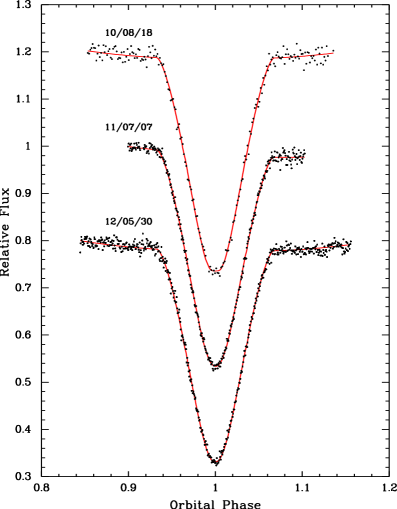
Figure 1: Primary eclipse of NSVS 1425 folded on the binary orbital period. The solid line represents the best fitting performed with the Wilson-Devinney code (see Section 3). The upper and lower light curves were displaced vertically 0.2 units for better visualization.

The data reduction was performed using iraf tasks (Tody, 1993) and consists of subtracting a master median bias image from each program image, and dividing the result by a normalized flat-field frame. Differential photometry was used to obtain the flux ratio between the target and a field star of assumed constant flux. As the NSVS 1425 field is not crowded, flux extraction was performed using aperture photometry. This procedure was repeated several times using different apertures and sky ring sizes to select the combination that provides the best signal-to-noise ratio. Figure 1 shows three normalized light curves folded on the NSVS 1425 orbital period.

3 ANALYSIS AND RESULTS

3.1 Eclipse fitting

To obtain the mid-eclipse times for NSVS 1425, we generated model light curves using the Wilson-Devinney code (WDC – Wilson & Devinney 1971) and searched for the best fit to the observed data. We used mode 2 of the WDC, which is appropriate to detached systems. The luminosity of each component was computed assuming stellar atmosphere radiation. The linear limb darkening coefficients, $x_{i}$, were used for both components. For the unfiltered light curves, $V$-band limb darkening was used. The ranges of the geometrical and physical parameters (e.g., inclination, radii, temperatures and masses) obtained by Almeida et al. (2012) for NSVS 1425 were adopted as the search intervals in the fit.

A method similar to that described in Almeida et al. (2012) was used for the fitting procedure. The WDC was used as a “function” to be optimized by the genetic algorithm pikaia (Charbonneau, 1995). To measure the goodness of fit, we use the reduced $\chi_{\rm red}^{2}$ defined as

$$\chi^{2}_{\rm red}=\frac{1}{n}\sum_{j=1}^{n}\left(\frac{O_{j}-C_{j}}{\sigma_{j}}\right)^{2},$$ (1)

where $O_{j}$ are the observed points, $C_{j}$ are the corresponding models, $\sigma_{j}$ is the uncertainty at each point, and $n$ is the number of points. Figure 1 shows three eclipses of NSVS 1425 and the corresponding best solutions. To establish realistic uncertainties, we used the solution obtained by pikaia as input to a Markov Chain Monte Carlo (MCMC) procedure (Gilks et al., 1996) and examined the marginal posterior distribution of probability of the parameters. The mid-eclipse times and corresponding uncertainties were obtained from the median value of the marginal distribution of the fitted times and the 1-$\sigma$ uncertainties from the corresponding 68% area under the distribution. The results are presented in Table Two possible circumbinary planets in the eclipsing post-common envelope system NSVS 14256825, together with previously published timings.

3.2 Linear ephemeris

To determine an ephemeris for the NSVS 1425 orbital period, we analyzed our measurements together with all available eclipse times in the literature after converting them to barycentric dynamical time (TDB). Table Two possible circumbinary planets in the eclipsing post-common envelope system NSVS 14256825 shows all eclipse times available for NSVS 1425. Fitting the data using a linear ephemeris, $T_{\rm min}=T_{0}+E\times P_{\rm bin}$, we obtain

$$T_{\rm min}={\rm TDB}\,2454274.2086(1)+0.110374165(1)\times E,$$ (2)

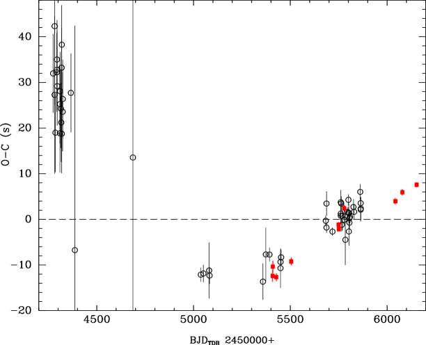
Figure 2: (O$-$C) diagram of the eclipse timings of NSVS 1425 made using Eq. 2. Our data are presented with full squares.

where $T_{\rm min}$ are the predicted eclipse times, $T_{\rm 0}$ is a fiducial epoch, $E$ is the cycle count from $T_{0}$ and $P_{\rm bin}$ is the binary orbital period. The best fit yields a $\chi^{2}_{\rm red}\sim 46$. The residuals of the observed times with respect to Eq. 2 are shown in the (O$-$C) diagram of Fig. 2

3.3 Eclipse timing variation

Figure 2 shows that a linear ephemeris is far from predicting correctly the NSVS 1425 eclipse times. The large value of $\chi^{2}_{\rm red}$ suggests the presence of additional signals in the (O$-$C) diagram. One possible explanation is the light travel time (LTT) effect, which is explored in this paper.

The LTT effect shows up as a periodic variation in the observed eclipse times when the distance from the binary to the observer varies due to gravitational interaction between the inner binary and an external body (Irwin, 1952). To fit the NSVS 1425 eclipse times taking this effect into account, we used the following equation,

$$T_{\rm min}=T_{0}+E\times P_{\rm bin}+\sum_{n=1}^{n}\tau_{j},$$ (3)

where

$$\tau_{\rm j}=\frac{z_{j}}{c}=K_{\rm j}\left[\frac{1-e^{2}_{j}}{1+e_{j}\cos f_{j}}\sin(f_{j}+\omega_{j})\right]$$ (4)

is the LTT effect. In the last equation, $K_{j}=a_{j}\sin i_{j}/c$ is the time semi-amplitude, $e_{j}$ is the eccentricity, $\omega_{j}$ is the argument of periastron, and $f_{j}$ is the true anomaly. These parameters are relative to the orbit of the inner binary center of mass around the common center of mass consisting of the inner binary and of the $j-$th planet. The parameters $a_{j}$, $i_{j}$, and $c$ in the semi-amplitude equation are the semi-major axis, the inclination, and the speed of light, respectively. Notice that we do not consider mutual interaction between external bodies in this analysis.

Initially we fitted Eq. 3 to the data with only one LTT effect. The resulting $\chi_{\rm red}^{2}$ dropped to 6.8, but the new residuals showed evidences of another cyclic variation. Adding one more LTT effect in Eq. 3, the resulting $\chi^{2}_{\rm red}$ improves to 1.85. The pikaia algorithm was used to search for the global optimal solution, followed by a MCMC procedure to sample the parameters of Eq. 3 around the best solution. Figure 3 shows the resulting (O$-$C) diagram and Table 4 shows the best fit parameters with the associated $\pm 68\%$ uncertainties.

4 DISCUSSION AND CONCLUSION

We revisited the orbital period variation of the post-CE binary NSVS 1425 adding the 10 new mid-eclipse times obtained as described in previous sections. The complex orbital period variation, illustrated by the (O$-$C) diagram, can be mathematically described by the LTT effect of two circumbinary objects. The amplitudes of the LTT effects are $\sim 20$ s and $\sim 5~{}s$. The associated orbital periods correspond to $\sim 6.9$ and $\sim 3.5$ years, respectively. This solution is a good description for the orbital period variation, as shown by Fig. 3. But it raises some concerns, which are discussed below.

The time baseline of NSVS 1425 covers about 5.5 years. One of the two LTT effects has a period of $\sim 7~{}$ years, larger than the baseline making the obtained solution less robust. Moreover, the early points have large errorbars and hence constrain less the LTT effect. In this regard, it is useful to recall the case of HW Vir. It is a similar system, which also presents a complex (O$-$C) diagram. Kilkenny et al. (2003), based on a dataset spread over almost 20 years, proposed the presence of a brown dwarf around the central binary. A few years later, a solution considering two objects was presented by Lee et al. (2009). Recently, Horner et al. (2012) claimed a still different solution, more stable dynamically. This illustrates how new data can change a LTT effect solution. Therefore, the LTT solution derived for NSVS 1425 should be considered as a preliminary one.

We now discuss the implications of the presence of two circumbinary objects in NSVS 1425. Using the close binary mass $M_{\rm bin}~{}=~{}0.528M_{\odot}$ (Almeida et al., 2012), the lower mass limit for the two circumbinary bodies are $M_{c}\sin i_{c}\sim 2.9~{}M_{\rm Jupiter}$ (inner body) and $M_{d}\sin i_{d}\sim 8.0~{}M_{\rm Jupiter}$ (external body). Assuming an orbital inclination of $82.5$ degrees (Almeida et al., 2012) and coplanarity between the two external bodies and the inner binary, NSVS 1425 c and NSVS 1425 d would both be giant planets with $M_{c}\sim 2.9~{}M_{\rm Jupiter}$ and $M_{d}\sim 8.1~{}M_{\rm Jupiter}$.

Considering NSVS 1425 with two circumbinary planets, this system would be the eighth post-CE system with planets and the fourth system with two planets (see Table 1). In such systems, there are two principal scenarios for planetary formation: (i) first generation planets formed in a circumbinary protoplanetary disk; and (ii) second generation planets originated from a disk formed by the ejected envelope (van Winckel et al., 2009; Perets, 2011).

In the first scenario, could the two circumbinary planets in NSVS 1425 survive the CE phase? Bear & Soker (2011) estimated the orbital separation between the progenitor of an extreme horizontal branch (EHB) star (sdB or sdOB) and a planet before the CE phase by the equation, $a_{0}\simeq M_{\rm EHB}a_{\rm EHB}/M_{\rm pro}$, where $M_{\rm EHB}$ is the mass of the sdOB star, and $a_{\rm EHB}$ is the present orbital separation of the planet. Assuming that the progenitor of the sdOB star in NSVS 1425 had a mass of $M_{\rm pro}=1.0\,M_{\odot}$, and neglecting accretion by the companion, the orbital separation of the planets before the CE would be $a_{0c}\simeq 0.8$ AU and $a_{0d}\simeq 1.3$ AU. For a single star, Han et al. (2002) pointed out that the maximum radius at the tip of the EHB ($R_{\rm EHB}$) is $\sim 0.8$ AU. Hence, the inner planet is on the verge of being engulfed by the CE. Moreover, the tidal interaction causes a planet to spiral inwards if its orbital radius is smaller than $a_{0}\lesssim 3\,R_{\rm EHB}$ (Villaver & Livio, 2007). Therefore the two circumbinary bodies in NSVS 1425 would not survive the CE phase. On the other hand, Taam & Ricker (2010) showed that the CE size can be much reduced if the EHB star is part of a binary system, because once the secondary is engulfed by the envelope, the CE is totally ejected in only $\sim 10^{3}$ days, stopping the envelope expansion. Therefore, the maximum radius of the CE is around the initial distance between the close binary components. Thus, if the close binary separation in NSVS 1425 before the CE phase was $\lesssim 0.27$ AU, the two planets could survive the CE phase.

For the second scenario, the principal question to investigate is: was there time enough after the CE phase to form giant planets? Kley (1999) showed that the typical time scale to form giant planets in protostellar disks is $\sim 10^{6}$ years. The lifetime of a binary in the EHB phase is $\sim 10^{8}$ years (Dorman et al., 1993; Heber, 2009). As the NSVS 1425 primary star is in the post-EHB phase (Almeida et al., 2012), we conclude that there was time enough to form the two circumbinary planets after the CE phase. Therefore the second generation of planets is also a viable scenario for NSVS 1425.

Finally, among all known candidates to be circumbinary planets in post-CE systems, the inner planet in NSVS 1425 has the minimum binary-planet separation, $a_{c}\sin i_{c}\sim 1.9$ AU.

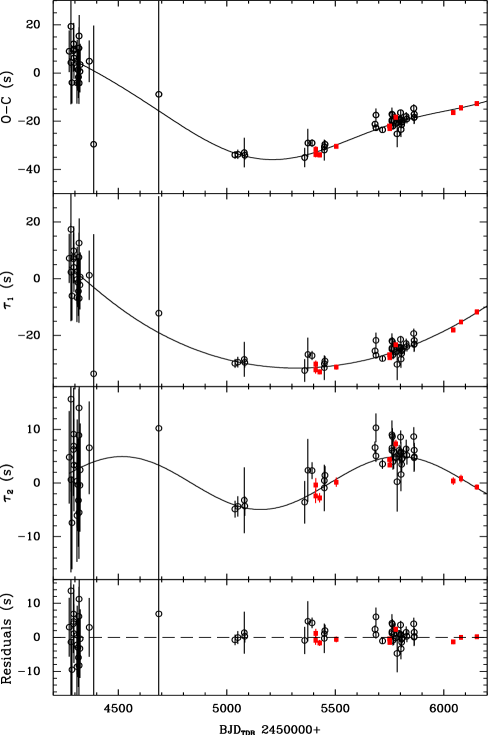
Figure 3: The upper panel shows the (O$-$C) diagram of the eclipse times of NSVS 1425 made with respect to the linear part of the ephemeris in Eq. 3. Our data are presented with full squares and the solid line represents the best fit including the two LTT effects. The second and third panels display separately the two LTT effects ($\tau_{1}$ and $\tau_{2}$). The lower panel shows the residuals around the combined fit.

Table 1: Circumbinary planets discovered in post-common envelope systems.

Name	$P_{\rm orb}$	$M_{\rm p}\sin i$	$a\sin i$	e	Spec. Type	References
	days	$M_{\rm Jupiter}$	AU
NSVS 1425(AB)c	1276	2.9	1.9	0.0	sdOB+dM	this study
UZ For(AB)c	1917	7.7	2.8	0.05	DA+dM (Polar)	1
HU Aqr(AB)c	2226	4.5	3.32	0.11	DA+dM (Polar)	2
NSVS 1425(AB)d	2506	8.0	2.9	0.52	sdOB+dM	this study
NN Ser(AB)c	2605	4.0	3.2	0.05	DA+dM	3
NY Vir(AB)c	2900	2.3	3.3	–	sdB+dM	4
RR Cae(AB)c	4346	4.2	5.3	0.0	DA+dM	5
HW Vir(AB)c	4640	14.0	4.69	0.4	sdB+dM	6
HU Aqr(AB)d	5155	5.7	5.81	0.04	DA+dM (Polar)	2
NN Ser(AB)d	5571	6.71	5.32	0.22	DA+dM	3
UZ For(AB)d	5844	6.3	5.9	0.04	DA+dM (Polar)	1
DP Leo(AB)c	10227	6.05	8.18	0.39	DA+dM (Polar)	7

Table 2: Log of the photometric observations

Date	$N$	$t_{\rm exp}$(s)	Telescope	Filter
2010 Jul 30	300	20	0.6-m	RC
2010 Jul 31	450	20	0.6-m	RC
2010 Aug 18	800	10	0.6-m	RC
2010 Nov 20	350	20	0.6-m	IC
2011 Jul 06	1255	2	1.6-m	IC
2011 Jul 07	1300	1	1.6-m	Clear
2011 Aug 06	435	5	1.6-m	V
2012 Apr 24	1550	1.5	0.6-m	Clear
2012 May 30	600	3	0.6-m	Clear
2012 Aug 12	1330	2	1.6-m	IC

Table 3: Eclipse times for NSVS 1425

Cycle	Time (BJD–TDB)	O$-$C (s)	Eclipse	Ref.
1	2454274.2088(1)	9.0	I	1
72	2454282.1559(2)	19.4	I	1
73	2454282.2661(2)	4.3	I	1
108	2454286.1291(1)	-4.0	I	1
172	2454293.1932(1)	9.2	I	1
180	2454294.0762(1)	9.8	I	1
181	2454294.1866(1)	12.1	I	1
190	2454295.1799(1)	6.2	I	1
316	2454309.0870(1)	2.3	I	1
317	2454309.1973(1)	-4.1	I	1
325	2454310.0804(1)	5.1	I	1
362	2454314.1642(1)	1.3	I	1
380	2454316.1509(1)	-1.7	I	1
397	2454318.0274(1)	10.3	I	1
406	2454319.0206(1)	-4.2	I	1
407	2454319.1312(1)	15.4	I	1
443	2454323.1045(1)	0.7	I	1
452	2454324.0979(1)	3.5	I	1
832	2454366.0401(1)	4.9	I	1
1018	2454386.5693(6)	-29.6	I	2
3737	2454686.6769(5)	-8.8	I	2
6914	2455037.33534(2)	-34.0	I	2
7037	2455050.91137(2)	-33.7	I	2
7304	2455080.38128(7)	-33.0	I	2
7322	2455082.36800(2)	-34.1	I	2
9823.5	2455358.46897(5)	-35.0	II	2
9959	2455373.42474(7)	-29.1	I	2
10131	2455392.40910(2)	-29.0	I	2
10279	2455408.74442(2)	-33.7	I	this study
10287	2455409.62744(2)	-31.7	I	this study
10451	2455427.72877(1)	-34.0	I	this study
10646	2455449.25176(5)	-31.9	I	3
10647	2455449.36215(2)	-30.6	I	3
10673	2455452.23189(2)	-29.6	I	3
11146.5	2455504.49405(1)	-30.4	II	this study
12763	2455682.91400(2)	-21.2	I	2
12799	2455686.88745(2)	-22.7	I	2
12799.5	2455686.94270(3)	-17.4	II	2
13077	2455717.57146(1)	-23.5	I	3
13368	2455749.690361(6)	-22.0	I	this study
13377	2455750.683717(4)	-23.0	I	this study
13629	2455778.498061(9)	-18.3	I	this study
13469	2455760.83818(3)	-19.6	I	2
13469.5	2455760.89340(3)	-17.1	II	2
13470	2455760.94855(1)	-20.0	I	2
13488	2455762.93532(2)	-17.3	I	2
13511	2455765.47387(2)	-22.0	I	2
13542	2455768.89549(4)	-20.0	I	2
13632	2455778.82915(1)	-20.9	I	2
13682	2455784.34781(7)	-25.2	I	2
13768	2455793.84006(1)	-19.2	I	2
13827	2455800.35217(2)	-16.5	I	2
13828	2455800.46251(2)	-19.2	I	2
13845	2455802.33887(5)	-19.4	I	2
13846	2455802.44920(4)	-23.4	I	2
13872	2455805.31896(2)	-20.5	I	2
13873	2455805.42932(2)	-21.5	I	2
13899	2455808.29907(2)	-20.2	I	2
14062	2455826.29008(2)	-18.0	I	3
14089	2455829.27017(2)	-19.1	I	3
14379	2455861.27873(2)	-14.6	I	3
14397	2455863.26542(3)	-18.5	I	3
14400	2455863.59656(1)	-17.1	I	2
14406	2455864.25879(3)	-18.3	I	3
16024	2456042.844216(4)	-16.4	I	this study
16350	2456078.826240(8)	-14.4	I	this study
17019	2456152.666554(6)	-12.6	I	this study

References. — (1) Potter et al. (2011); (2) Hinse et al. (2012); (3) Horner et al. (2012); (4) Qian et al. (2012a); (5) Qian et al. (2012b); (6) Beuermann et al. (2012a); (7) Beuermann et al. (2011).

References. — (1) Wils et al. (2007); (2) Beuermann et al. (2012a); (3)Kilkenny & Koen (2012).

Table 4: Parameters for the linear plus two-LTT ephemeris of NSVS 1425.

	Linear ephemeris
Parameter	Value	Unit
$P_{\rm bin}$	0.1103741681(5)	days
$T_{0}$	2454274.20874(4)	BJD(TDB)
	$\tau_{1}$ term
Parameter	Value	Unit
$P$	$6.86\pm 0.45$	years
$T$	$2456643\pm 110$	BJD(TDB)
$a_{\rm bin}\sin i$	$0.042\pm 0.006$	AU
$e$	$0.52\pm 0.08$
$\omega$	$98\pm 9$	degrees
$f(M)$	$(1.6\pm 1.1)\times 10^{-6}$	$M_{\odot}$
$M\sin i$	$8.0\pm 1.5$	$M_{\rm Jupiter}$
$a\sin i$	$2.9\pm 0.7$	AU
	$\tau_{2}$ term
Parameter	Value	Unit
$P$	$3.49\pm 0.38$	years
$T$	$2455515\pm 95$	BJD(TDB)
$a_{\rm bin}\sin i$	$0.0099\pm 0.0006$	AU
$e$	$0.00\pm 0.08$
$\omega$	$11\pm 8$	degrees
$f(M)$	$(8.0\pm 4.0)\times 10^{-8}$	$M_{\odot}$
$M\sin i$	$2.9\pm 0.4$	$M_{\rm Jupiter}$
$a\sin i$	$1.9\pm 0.8$	AU
$\chi^{2}_{\rm red}$	1.85

References

- Almeida et al. (2012) Almeida, L. A., Jablonski, F., Tello, J., & Rodrigues, C. V. 2012, MNRAS, 423, 478
- Backer et al. (1993) Backer, D. C., Foster, R. S., & Sallmen, S. 1993, Nature, 365, 817
- Bear & Soker (2011) Bear, E., & Soker, N. 2011, MNRAS, 411, 1792
- Beuermann et al. (2011) Beuermann, K., Buhlmann, J., Diese, J., et al. 2011, A&A, 526, A53
- Beuermann et al. (2012a) Beuermann, K., Dreizler, S., Hessman, F. V., & Deller, J. 2012a, A&A, 543, A138
- Beuermann et al. (2012b) Beuermann, K., Breitenstein, P., Bski, B. D., et al. 2012b, A&A, 540, A8
- Charbonneau (1995) Charbonneau, P. 1995, ApJS, 101, 309
- Dorman et al. (1993) Dorman, B., Rood, R. T., & O’Connell, R. W. 1993, ApJ, 419, 596
- Gilks et al. (1996) Gilks, W. R., Richardson, S., & Spiegelhalter, D. J. E. 1996, Markov Chain Monte Carlo in Practice, Chapman & Hall, London
- Han et al. (2002) Han, Z., Podsiadlowski, P., Maxted, P. F. L., Marsh, T. R., & Ivanova, N. 2002, MNRAS, 336, 449
- Heber (2009) Heber, U. 2009, ARA&A, 47, 211
- Hinse et al. (2012) Hinse, T. C., Lee, J. W., Goździewski, K., et al. 2012, MNRAS, 420, 3609
- Horner et al. (2012) Horner, J., Wittenmyer, R. A., Hinse, T. C., & Tinney, C. G. 2012, MNRAS, 425, 749
- Kilkenny et al. (2003) Kilkenny, D., van Wyk, F., & Marang, F. 2003, The Observatory, 123, 31
- Kilkenny & Koen (2012) Kilkenny, D., & Koen, C. 2012, MNRAS, 421, 3238
- Kley (1999) Kley, W. 1999, MNRAS, 303, 696
- Irwin (1952) Irwin, J. B. 1952, ApJ, 116, 211
- Lee et al. (2009) Lee, J. W., Kim, S.-L., Kim, C.-H., et al. 2009, AJ, 137, 3181
- Moriwaki & Nakagawa (2004) Moriwaki, K., & Nakagawa, Y. 2004, ApJ, 609, 1065
- Perets (2011) Perets, H. B. 2011, American Institute of Physics Conference Series, 1331, 56
- Potter et al. (2011) Potter, S. B., Romero-Colmenero, E., Ramsay, G., et al. 2011, MNRAS, 416, 2202
- Qian et al. (2012a) Qian, S.-B., Zhu, L.-Y., Dai, Z.-B., et al. 2012a, ApJ, 745, L23
- Qian et al. (2012b) Qian, S.-B., Liu, L., Zhu, L.-Y., et al. 2012b, MNRAS, 422, L24
- Quintana & Lissauer (2006) Quintana, E. V., & Lissauer, J. J. 2006, Icarus, 185, 1
- Taam & Ricker (2010) Taam, R. E., & Ricker, P. M. 2010, New A Rev., 54, 65
- Tody (1993) Tody, D. 1993, Astronomical Data Analysis Software and Systems II, 52, 173
- van Winckel et al. (2009) van Winckel, H., Lloyd Evans, T., Briquet, M., et al. 2009, A&A, 505, 1221
- Villaver & Livio (2007) Villaver, E., & Livio, M. 2007, ApJ, 661, 1192
- Wils et al. (2007) Wils, P., di Scala, G., & Otero, S. A. 2007, Information Bulletin on Variable Stars, 5800, 1
- Wilson & Devinney (1971) Wilson, R. E., & Devinney, E. J. 1971, ApJ, 166, 605
- Woźniak et al. (2004) Woźniak, P. R., Williams, S. J., Vestrand, W. T., & Gupta, V. 2004, AJ, 128, 2965