Quantum statistical imaging of particles without restriction of the diffraction limit

Abstract

A quantum measurement method based on the quantum nature of anti-bunching photon emission has been developed to detect single particles without the restriction of the diffraction limit. By simultaneously counting the single-photon and two-photon signals with fluorescence microscopy, the images of nearby Nitrogen-Vacancy centers in diamond at a distance of $8.5\pm 2.4$ nm have been successfully reconstructed. Also their axes information was optically obtained. This quantum statistical imaging technique, with a simple experimental setup, can also be easily generalized in the measuring and distinguishing of other physical properties with any overlapping, which shows high potential in future image and study of coupled quantum systems for quantum information techniques.

The measurement of physical quantities is not only a major goal but also an active impulsion for scientific research. Especially, the imaging of nearby particles is important for modern science Alivisatos ; Patterson . The precision with which two nearby particles can be resolved is classically restricted by the optical diffraction limit. Imaging methods that used distinguishing information based on the photons emitted from different particles have been proposed to achieve precision beyond the diffraction limit Ash ; Denk ; Klar ; Rust ; Betzig ; Hess ; Dertinger . When the emitted photons have the same properties, distinguishing nearby particles which are separated by distances much less than the diffraction limit is difficult.

Recently, phenomena from quantum mechanics have been used to improve the measurement and applied to some special purposes which cannot be performed by classical method. Such quantum techniques are being applied to enhance the precision of measurements beyond the classical limit Giovannetti ; LIGO . However, many quantum-based protocols to improve the measurement used the quantum entanglement. They are fragile because of quantum decoherence Nagata ; Sun ; Xiang . For practical purpose, stable quantum phenomena should be applied in the measurement. There are proposals to enhance the imaging resolution based on the quantum statistics Dertinger ; Schwartz . Here, we have developed a quantum statistical imaging (QSI) method to detect single particles without the restriction of the diffraction limit. In the quantum regime, the situation for particles imaging is different because each particle emits only one photon and shows the single-photon antibunching effect Kimble . By detecting the photon coincident counts, the particles can be imaged and resolved even when they are almost completely overlapping and the emitted photons are identical. Here, Nitrogen-vacancy center (NVC) in diamond was used in this experimental demonstration. Single NVC has shown its good quality as a single-photon source Kurtsiefer ; Babinec . When two NVCs are close to each other, i.e., within tens of nanometers, the strong dipole-dipole interaction can be applied in quantum information techniques Maurer ; Neumann . Diamond nano-crystals with NVCs have been successfully used to image biological processes Chang ; McGuinness . The ability to image and distinguish two nearby NVCs is becoming increasingly important in physics Maurer ; Neumann ; Rittweger and biology Chang ; McGuinness .

NVCs are usually detected by scanning confocal optical fluorescence microscopy Gruber , in which the single-photon intensity of spontaneous emission is measured to characterize the optical images of the centers. The spontaneous emission from the NVCs, which were fabricated by nitrogen ions implantation, is collected into a single-mode fiber. The collected photons are then split into two paths by a fiber beam splitter with a transmissivity of T and a reflectivity of R ($T+R=1$), to form a Hanbury-Brown-Twiss interferometer HBT . Finally, the separated beams are detected with two single-photon detectors. When two NVCs ($A$ and $B$) are imaged, the single-photon intensity at position ($x$, $y$) from the single-photon detectors $D_{1}$ and $D_{2}$ can be expressed as

$$\left\langle I_{1}^{D1}(x,y)\right\rangle = T[\left\langle I_{A}(x,y)\right\rangle+\left\langle I_{B}(x,y)\right\rangle]\text{,}$$

$$\left\langle I_{1}^{D2}(x,y)\right\rangle = R[\left\langle I_{A}(x,y)\right\rangle+\left\langle I_{B}(x,y)\right\rangle]\text{,}$$

where $\left\langle I_{A}(x,y)\right\rangle$ and $\left\langle I_{B}(x,y)\right\rangle$ are the single-photon rates from NVCs $A$ and $B$, respectively. Therefore, the single photons from the two NVCs are

$$\left\langle I_{1}(x,y)\right\rangle = \left\langle I_{1}^{D1}(x,y)\right\rangle+\left\langle I_{1}^{D2}(x,y)\right\rangle$$ (1)

$$= \left\langle I_{A}(x,y)\right\rangle+\left\langle I_{B}(x,y)\right\rangle\text{.}$$

When the distance between the two NVCs is within the optical diffraction limit, $\left\langle I_{A}(x,y)\right\rangle$ and $\left\langle I_{B}(x,y)\right\rangle$ are overlapping and hardly distinguishable from the single-photon intensity $\left\langle I_{1}(x,y)\right\rangle$. If two-photon coincident counts are measured, then the two photons must come from two NVCs and never from the same NVC because a single NVC only emits one photon. This attribute demonstrates a genuine quantum characteristic, namely, the photon anti-bunching effect with $\left\langle:[I_{A}(x,y)]^{2}:\right\rangle=\left\langle:[I_{B}(x,y)]^{2}:\right\rangle=0$, where $::$ represents normal ordering QO . Therefore, the two-photon intensity will be

$$\left\langle I_{2}(x,y)\right\rangle=\eta_{2}(1+K)RT\left\langle I_{A}(x,y)\right\rangle\left\langle I_{B}(x,y)\right\rangle\text{,}$$ (2)

where $\eta_{2}$ is the two-photon detection constant, which is based on the imperfections from the photon collection efficiency, path loss, detection efficiency of the single-photon detectors and coincident detection windows in the experiment. $K$ describes the quantum indistinguishability-induced bunching effect of two photons Santori ; Sun09 . Usually, $K=0$ in many measurements without special spectral filtering. For example, the photon from NVC has very broad phonon bandwidth comparing to its narrow zero-phonon line width Gruber , leading $K=0$ in the present measurement. Therefore, simply from $\left\langle I_{1}(x,y)\right\rangle$ and $\left\langle I_{2}(x,y)\right\rangle$, the values of $\left\langle I_{A}(x,y)\right\rangle$ and $\left\langle I_{B}(x,y)\right\rangle$ can be obtained, even if they are completely overlapping. Subsequently, the optical images of the two NVCs can be reconstructed and distinguished. For $N$ particles, $m$-th ($1\leqslant m\leqslant N$) order coincidence measurement will give

$$\left\langle I_{m}(x,y)\right\rangle=\eta_{m}\mathop{\displaystyle\sum}[\left\langle I_{A}(x,y)\right\rangle\left\langle I_{B}(x,y)\right\rangle...]_{m\text{ different points}}\text{,}$$

where $\eta_{m}$ is the $m$-photon detection constant and the photon indistinguishability induced photon bunching effect is also neglected. There are $N$ independent values, where images of each particles can be solved and reconstructed. There is no need to have any assumption on the distribution function of the image or the point spread function Schwartz . This technique utilizes a genuine quantum phenomenon to produce this result without classical parallelism.

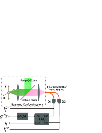
Figure 1: (color online) Schematic of measurement setup. Confocal NV fluorescent photons are splitted by a fiber beam splitter and sent to single photon detectors $D1$ and $D2$. TAC is used to get coincidence counts and MCA is to implement autocorrelation measurement ($g_{c}^{(2)}(\tau)$). $I_{1}^{D1}$, $I_{1}^{D1}$, and $I_{2}$ are $D1$, $D2$ and coincidence count rates, respectively.

In the experiment, NVCs are excited by a continuous $532$ nm green laser, and the experimental setup is shown in Fig. 1. To record the two-photon counting rate $\left\langle I_{2}\right\rangle$ at the same time, a single-channel analyzer (SCA) on a time-amplitude converter (TAC) is used to obtain the coincidence counts of $D1$ and $D2$, with a SCA window width of $t_{w}=2$ ns at $\tau=0$ because a single NV center has an anti-bunching decay with a width of approximately $20$ ns. The two-photon autocorrelation measurement ($g_{c}^{(2)}(\tau)$) is performed by the multi-channel analyzer (MCA). Using scanning confocal microscopy, $\left\langle I_{1}\right\rangle$ and $\left\langle I_{2}\right\rangle$ for each position are recorded to construct single-photon and two-photon images. The coincidence measurement is conducted in start-stop mode in the TAC, and

$$\eta_{2}=\frac{2t_{w}\left\langle I_{1}^{D1}\right\rangle\left\langle I_{1}^{D2}\right\rangle}{RT(\left\langle I_{1}^{D1}\right\rangle+\left\langle I_{1}^{D2}\right\rangle)^{2}}\text{,}$$

with $R=54\%$ and $T=46\%$.

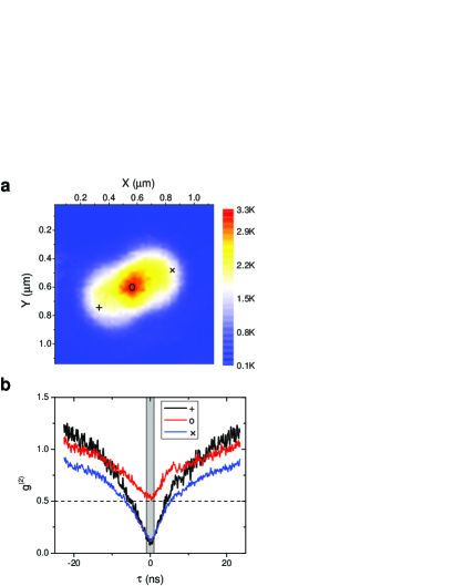
Figure 2: (color online) (a) Confocal image of two NVCs apart from $366.1$ nm. (b) $g_{c}^{(2)}(\tau)$ at different points in (a). The gray window indicates the SCA window $t_{w}=2\mathrm{ns}$ to measure $I_{2}$.

Two nearby two-NVC pairs were measured. Fig. 2 (a) displays a confocal scanning image of the first two-NVC pair. Fig. 2 (b) displays $g_{c}^{(2)}(\tau)$ with background noise subtraction. The position with maximal intensity marked as “$\circ$” is at the overlapping area of two NVCs, where both NVCs are excited in the pump focus with $g_{c}^{(2)}(0)$ is about $0.5$. However, while the confocal spot is on side position marked as “$+$” or “$\times$”, only one NVC are effectively excited as another NVC is out of exciton spot. Therefore, $g_{c}^{(2)}(0)$ is close to zero as a single NVC. From marked positions “$+$” to “$\circ$” in Fig. 2 (a), it is clear to see the variation from single to double NVCs.

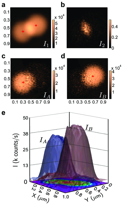
Figure 3: (color online) Optical images of two single NVCs at a distance of $366.1\pm 2.8$ nm. (a) and (b) show $I_{1}$ and $I_{2}$ for the single-photon and two-photon counts. (c) and (d) are images of each NVC ($I_{A}$, $I_{B}$), respectively. The red crosses mark the positions of the NVCs with an uncertainty of $1/20$ the length of each cross. The positions were obtained using a two-dimensional (2D) Gaussian fitting of $I_{A}$ or $I_{B}$. (e) A 3D image of the two NVCs.

For the first pair, the single-photon intensity (($\left\langle I_{1}(x,y)\right\rangle$) and two-photon intensity ($\left\langle I_{2}(x,y)\right\rangle$) were recorded at the same time (Fig. 3 (a, b)). In Fig. 3 (b), the image of the two-photon intensity has a narrower width in the overlapping region of the two NVCs. However, these images do not provide spatially resolved images of the two NV centers. The image of a single NVC should have a single peak and a continuous envelope. Using $\left\langle I_{1}(x,y)\right\rangle$ and $\left\langle I_{2}(x,y)\right\rangle$, the photon intensities $\left\langle I_{A}(x,y)\right\rangle$ and $\left\langle I_{B}(x,y)\right\rangle$ of the two particles can be obtained by solving Eq. (1) and Eq. (2). The images of the two particles, $I_{A}$ and $I_{B}$, were reconstructed and are shown in Fig. 3(c, d). By fitting the data, the distance between the NVCs was determined to be $366.1\pm 2.8$ nm, which is at the edge of the diffraction limit. Fig. 3 (e) shows a three-dimensional (3D) image of the two nearby NVCs, and the overlapping can be observed.

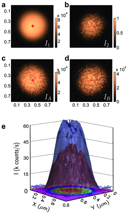
Figure 4: (color online) Optical imaging of two single NVCs with a small separation. The images are organized as in Fig.3. The distance between the NVCs was determined to be $8.5\pm 2.4$ nm by fitting $I_{A}$ and $I_{B}$.

Another pair of NVCs with a much smaller separation was also measured and distinguished. The confocal scanning image, the result of photon autocorrelation measurement and the spectrum show that there are two NVCs (see Supplementary Figure S2). The single-photon and two-photon images are shown in Fig. 4 (a, b). From the single-photon intensity, the two NVCs are well overlapping and cannot be distinguished. Using the QSI method, their images, $I_{A}$ and $I_{B}$, can be obtained, shown in Fig. 4 (c, d). The distance between the centers was determined to be $8.5\pm 2.4$ nm by fitting $I_{A}$ and $I_{B}$. This distance is much smaller than the diffraction limit, and the NVCs cannot be readily distinguished by the classical method Maurer . Here, the resolution (see Supplementary for details) was determined by the number of recorded photons and the experimental setup. In the present measurement, the error is about $0.9$ nm with $10^{5}$ coincident photon counts and the setup repeat resolution for $x$ or $y$ axis is about $0.7$ nm.

Besides imaging nearby particles, such a quantum measurement method can be easily generalized to measure and distinguish other properties even with high overlapping. For example, the axes of the NVCs can be measured. The spontaneous emission rates vary with the polarization of the pump beam according to different axes of NVCs Epstein ; Alegre . With polarized optical pump for our [100]-oriented sample, number of possible orientations of a given center is reduced from four to two, which are in the plane of $\varphi=0^{\circ}$ or $\varphi=90^{\circ}$ as shown in Fig. 5 (a). Here with QSI, the axes of the pair of NVCs at the distance of $8.5$ nm have been obtained. With different polarized pump beam, the single-photon and two-photon counts are shown in Fig. 5 (b). Simply, the emission intensity of each NVCs with the angle of polarization can be obtained in Fig. 5 (c). Correspondingly, the axes of the two NVCs are same in the plane of $\varphi=0^{\circ}$. The data can be fitted with $I_{A(B)}=\alpha_{A(B)}+\beta_{A(B)}\cos^{2}\varphi$ Alegre with $\alpha_{A(B)}=37.5\pm 0.4(23.1\pm 0.5)$ and $\beta_{A(B)}=-21.0\pm 0.8(-10.8\pm 0.9)$. The small dip at $\varphi=90^{\circ}$ for NV_B may come from its depth in the diamond Epstein .

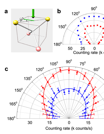
Figure 5: (color online) (a) The schematic of two sets of axes for [100]-oriented NVC sample according to the polarization of pump beam. They are in the plane of $\varphi=0^{\circ}$ or $\varphi=90^{\circ}$. (b) Single-photon and two-photon emission intensity versus the polarization angle of pump beam. The two-photon intensity was amplified by $5\times 10^{3}$ for view. (c) Separated intensities of two NVCs versus the polarization angle of pump beam.

In addition to the demonstrated symmetric envelopes of the photons from NVCs, the QSI method can be applied to detect and distinguish images with other continuous envelopes. Furthermore, the QSI method can be used to detect other particles and distinguish other degrees of freedom, such as lifetime, frequency, and polarization. Because the photons from each particle can be recorded simultaneously and distinguished without decoupling nearby particles, the QSI method can be used to detect their separate dynamics, as well as the coupling between them. Also, the experimental setup for QSI is simple. It does not need complicated pump beams Maurer ; Rittweger or the assistance of other control systems Maurer ; Neumann . In the current experiment, the single-photon counts were about $20\mathrm{K/s}$ and the total detection efficiency was about $0.15\%$, including the loss at the collection objective ($97\%$), pass loss ($90\%$) and the loss at the detector ($50\%$). However, in principle, all of these performances can be much improved. The collection efficiency can be enhanced by a factor of $8$ with structured interface Marseglia . The loss from beamsplitter can be removed with additional detectors Xiang . The loss at the detector can be overcome with high quantum efficiency. If pulsed laser is used, there is no need the $2\mathrm{ns}$ gate and all the photons within its lifetime can be collected, which is about $6$-fold enhancement in the two-photon counts. Along with other low loss filters, the total two-photon detection rate can be improved by over three orders of magnitude. For the image of NVCs, the sample was moved at $40\times 40$ locations (pixels) and photon counts were collected at each location. A gated CCD can be used to give additional enhancement in the data collection. With above improved techniques, the total data collection time will be less than one minute for the two NVCs with same resolution, compared to current $50$ hours. It is very promising in the scalable application for multi-partite measurement and the detection of particles which emit small numbers of photons because of bleaching or blinking. In those cases, the resolution is limited by the total photons. However, it will still have very good resolution. For example, $10^{5}$ photons can offer the sub-nanometer resolution.

In summary, a QSI method was demonstrated based on the unique quantum behavior of anti-bunching emission photons. Two well-overlapping NVCs can be spatially resolved. Also, the axes of the two NVCs are measured even their distance is within $8.5$ nm. With high order of coincident multi-photon measurements, additional single NVCs can be imaged and distinguished. The scalable QSI with high order coincidence counts will be applied in the multipartite interaction for quantum information techniques and modern physics.

- (1) P. Alivisatos, Nature Biotechnol. 22, 47 (2004).
- (2) G. Patterson, M. Davidson, S. Manley, and J. Lippincott-Schwartz, Annu. Rev. Phys. Chem. 61, 345 (2010).
- (3) E. A. Ash, and G. Nicholls, Nature 237, 510 (1972).
- (4) W. Denk, J. H. Strickler, and W. W. Webb, Science 248, 73 (1990).
- (5) T. A. Klar and S. W. Hell, Opt. Lett. 24, 954 (1999).
- (6) M. J. Rust, M. Bates, and X. Zhuang, Nature Meth. 3, 793 (2006).
- (7) E. Betzig, et. al., Science 313, 1642 (2006).
- (8) S. T. Hess, T. P. Girirajan, and M. D. Mason, Biophys. J. 91, 4258 (2006).
- (9) T. Dertinger, R. Colyer, G. Iyer, S. Weiss, and J. Enderlein, Proc. Natl. Acad. Sci. USA 106, 22287 (2009).
- (10) V. Giovannetti, S. Lloyd, and L. Maccone, Science 306, 1330 (2004).
- (11) The LIGO Scientific Collaboration, Nature Phys. 7, 962 (2011).
- (12) T. Nagata, R. Okamoto, J. L. O’Brien, K. Sasaki, and S. Takeuchi, Science 316, 726 (2007).
- (13) F. W. Sun, B. H. Liu, Y. X. Gong, Y. F. Huang, Z. Y. Ou, and G. C. Guo, EPL 82, 24001 (2008).
- (14) G. Y. Xiang, B. L. D. Higgins, W. H. Berry, M. G Wiseman, and J. Pryde, Nature Photon. 5, 43 (2011).
- (15) O. Schwartz and D. Oron, Phys. Rev. A 85, 033812 (2012).
- (16) H. J. Kimble, M. Dagenais, and L. Mandel, Phys. Rev. Lett. 39, 691 (1977).
- (17) C. Kurtsiefer, S. Mayer, P Zarda, and H. Weinfurter, Phys. Rev. Lett. 85, 290 (2000).
- (18) T. M. Babinec, et. al., Nature Nanotech. 5, 195 (2010).
- (19) P. C. Maurer, et. al., Nature Phys. 6, 912 (2010).
- (20) P. Neumann, et. al., Nature Phys. 6, 249 (2011).
- (21) Y. -R. Chang, et. al., Nature Nanotech. 3, 284 (2008).
- (22) L. P. McGuinness, et. al., Nature Nanotech. 6, 358 (2011).
- (23) E. Rittweger, D. Wildanger, and S. W. Hell, EPL. 86, 14001 (2009).
- (24) A. Gruber, et. al., Science 276, 2012 (1997).
- (25) R. Hanbury Brown and R. Q. Twiss, Nature 177, 27 (1956).
- (26) M. O. Scully, and M. S. Zubairy, Quantum Optics (Cambridge University Press 1997).
- (27) C. Santori, D. Fattal, J. Vučković, G. S. Solomon, and Y. Yamamoto, Nature 419, 594 (2002).
- (28) F. W. Sun and C. W. Wong, Phys. Rev. A 79, 013824 (2009).
- (29) R. J. Epstein, F. M. Mendoza, Y. K. Kato, and D. D. Awschalom, Nature Phys. 1, 94 (2005).
- (30) Thiago P. Mayer Alegre, C. Santori, G. Medeiros-Ribeiro, and R. G. Beausoleil, Phys. Rev. B 76, 165205 (2007).
- (31) L. Marseglia, et.al., Appl. Phys. Lett. 98, 133107 (2011).