Variational Downscaling, Fusion and Assimilation of Hydrometeorological States via Regularized Estimation

Abstract

Improved estimation of hydrometeorological states from down-sampled observations and background model forecasts in a noisy environment, has been a subject of growing research in the past decades. Here, we introduce a unified framework that ties together the problems of downscaling, data fusion and data assimilation as ill-posed inverse problems. This framework seeks solutions beyond the classic least squares estimation paradigms by imposing proper regularizations, which are constraints consistent with the degree of smoothness and probabilistic structure of the underlying state. We review relevant regularization methods in derivative space and extend classic formulations of the aforementioned problems with particular emphasis on hydrologic and atmospheric applications. Informed by the statistical characteristics of the state variable of interest, the central results of the paper suggest that proper regularization can lead to a more accurate and stable recovery of the true state and hence more skillful forecasts. In particular, using the Tikhonov and Huber regularizations in the derivative space, the promise of the proposed framework is demonstrated in static downscaling and fusion of synthetic multi-sensor precipitation data, while a data assimilation numerical experiment is presented using the heat equation in a variational setting.

1 Introduction

In parallel to the growing technologies for earth remote sensing, we have witnessed an increasing interest to improve the accuracy of observations and integrate them with physical models for more accurate estimates and forecasts of environmental states. Remote sensing observations are typically noisy and coarse-scale representations of a true state variable of interest, lacking sufficient accuracy and resolution for fine-scale environmental modeling. In addition, environmental predictions are not perfect as models often suffer either from inadequate characterization of the underlying physics or their initial conditions. Given these limitations, several classes of estimation problems present themselves as continuous challenges for the atmospheric, hydrologic and oceanic science communities. These include: (1) Downscaling which refers to the class of problems to enhance the resolution of a measured field or produce a fine-scale representation of a coarse-scale modeled field; (2) Data fusion, to produce an improved estimate from a suite of noisy observations at different scales; and (3) Data assimilation which deals with estimating initial conditions in a predictive model consistent with the available noisy observations and the model dynamics. In this paper, we revisit the problems of downscaling (DS), data fusion (DF), and data assimilation (DA) focusing on a common thread between them as inverse estimation problems. Proper regularizations and solution methods are proposed to efficiently handle large-scale data sets while preserving key statistical and geometrical properties of the underlying fields of interest. Here, we only examine hydrometeorological problems with particular emphasis on land-surface applications.

In land surface hydrologic studies, downscaling of precipitation and soil moisture signals has received considerable attention, using a relatively wide range of methodologies. DS methods in hydrometeorology and climate studies generally fall into three main categories namely, dynamic downscaling, statistical downscaling, and variational downscaling. Dynamic downscaling often uses a regional physical model to reproduce fine-scale details of the state of interest consistent with the large-scale scale observations or outputs of a global circulation model [e.g., Reichle et al., 2001a; Castro et al., 2005; Zupanski et al., 2010]. Statistical downscaling methods encompass a large group of methods that typically use empirical multiscale statistical relationships, parameterized by observations or other environmental predictors, to reproduce realizations of fine-scale fields. Precipitation and soil moisture statistical downscaling has been mainly approached via spectral and (multi)fractal interpolation methods, capitalizing on the presence of a power law spectrum and a statistical self-similarity/self-affinity in precipitation and soil moisture fields [among others, Lovejoy and Mandelbrot, 1985; Lovejoy and Schertzer, 1990; Gupta and Waymire, 1993; Kumar and Foufoula-Georgiou, 1993a, b; Perica and Foufoula-Georgiou, 1996; Veneziano et al., 1996; Wilby et al., 1998b, a; Deidda, 2000; Kim and Barros, 2002; Rebora et al., 2005; Badas et al., 2006; Merlin et al., 2006]. In variational approaches, a direct cost function is defined whose optimal point is the desired fine-scale field which can be obtained via using an optimization routine. Recently along this direction, Ebtehaj et al. [2012] cast the rainfall DS problem as an inverse problem using sparse regularization to address the intrinsic rainfall singularities and non-Gaussian statistics. This variational approach belongs to the class of methodologies presented and extended in this paper.

The DF problem has also been a subject of continuous interest in the precipitation science community mainly due to the availability of rainfall measurements from multiple spaceborne (e.g., TRMM and GOES satellites) and ground-based sensors (e.g., the NEXRAD network). The accuracy and space-time coverage of remotely sensed rainfall are typically conjugate variables. In other words, more accurate observations are often available with lower space-time coverage and vice verse. For instance, low-orbit microwave sensors provide more accurate with less space-time coverage compared to the high-orbit geo-stationary infrared (GOES-IR) sensors. Moreover, there are often, multiple instruments on a single satellite platform (e.g., precipitation radar and microwave imager on TRMM), each of which measures rainfall with different footprints and resolutions. A wide range of methodologies including weighted averaging, regression, filtering, and neural networks has been applied to combine microwave and Geo-IR rainfall signals [e.g., Adler et al., 2003; Huffman et al., 1995; Sorooshian et al., 2000; Huffman et al., 2001; Hong et al., 2004; Huffman et al., 2007]. Furthermore, a few studies have addressed methodologies to optimally combine the products of the TRMM precipitation radar (PR) with the TRMM microwave imager (TMI) using Bayesian inversion and weighted least squares approaches [e.g., Masunaga and Kummerow, 2005; Kummerow et al., 2010]. From another direction, Gaussian filtering methods on Markovian tree-like structures, the so-called scale-recursive-estimation (SRE), have been proposed to merge spaceborne and ground-based rainfall observations at multiple scales [e.g., Gorenburg et al., 2001; Tustison et al., 2003; Bocchiola, 2007; Van de Vyver and Roulin, 2009; Wang et al., 2011], see also [Kumar, 1999] for soil moisture application. Recently, using the Gaussian scale mixture probability model and an adaptive filtering approach Ebtehaj and Foufoula-Georgiou [2011b] proposed a fusion methodology in the wavelet domain to merge TRMM-PR and ground-based NEXRAD measurements, aiming to preserve the non-Gaussian structure and local extremes of precipitation fields.

Data assimilation has played an important role in improving the skill of environmental forecasts and has become by now a necessary step in operational prediction models [see Daley, 1993]. Data assimilation amounts to integrating the underlying knowledge from the observations into the first guess or the background state, typically provided by a physical model. The goal is then to obtain the best estimate of the current state of the system, the so called analysis. The analysis with reduced error is then used to forecast the state at the next time step and so on [see Daley, 1993; Kalnay, 2003, for a comprehensive review]. Note that, in practice, the present background state, used in each analysis cycle, is commonly a forecast of the state by the underlying model, initialized by the analysis state in the previous time step. One of the most common approaches to the data assimilation problem relies on variational techniques [e.g., Sasaki, 1958, 1970; Lorenc, 1986; Talagrand and Courtier, 1987; Courtier and Talagrand, 1990; Parrish and Derber, 1992; Zupanski, 1993; Courtier et al., 1994; Reichle et al., 2001b, among many others]. In these methods, one explicitly defines a cost function, typically quadratic, whose potentially unique minimizer is the analysis state. Very recently Freitag et al. [2012] proposed a regularized data assimilation scheme to improve assimilation results in advective sharp fluid fronts.

What is common in the DS, DF, and DA problems is that, in all of them, we seek an improved estimate of the true state given a suite of noisy and down-sampled observations and/or uncertain model-predicted states. Specifically, let us suppose that the unknown true state in continuous space is denoted by $x(t)$ and its indirect observation (or model-output), by $y(r)$. Let us also assume that $x(t)$ and $y(r)$ are related via a linear integral equation, called the Fredholm integral equation of the the first kind, as:

$$\int_{0}^{1}\mathcal{H}(r,\,t)\,x(t)\,dt=y(r),\,\,\,\,\,\,\,0\leq r\leq 1,$$ (1)

where $\mathcal{H}(r,\,t)$ is the kernel relating $x(t)$ and $y(r)$. Recovery of $x(t)$ knowing $y(r)$ and $\mathcal{H}(r,\,t)$ is a classic linear inverse problem. Clearly, the deconvolution problem is a very special case with the kernel of the form $\mathcal{H}(r-t)$, which in its discrete form, plays a central role in this paper. Linear inverse problems are by nature ill-posed, in the sense that they do not satisfy at least one of the following three conditions: (1) Existence; (2) Uniqueness; and (3) Stability of the solution. For instance, when due to the kernel architecture, the dimension of the observation is smaller than that of the true signal, infinite choices of $x(t)$ lead to the same $y(r)$ and there is no unique solution for the problem. For the case when $y(r)$ is noisy and has a larger dimension than the true state, the solution is typically very unstable, because, the high frequency components in $y(r)$ are typically amplified and spoil the solution. In fact, the higher the frequency, the larger the amplification in the solution, which is often called the inverted noise; see, e.g., Hansen [2010] for a comprehensive account on linear inverse problems. A common approach to make an inverse problem well-posed is via the so-called regularization methods. The goal of regularization is to reformulate the inverse problem aiming to obtain a unique and sufficiently stable solution. The choice of regularization typically depends on the continuity and degree of smoothness of the state variable of interest, often called the regularity condition. For instance, some state variables are very regular with high degree of smoothness (e.g., pressure) while others might be more irregular and suffer from frequent and different sorts of discontinuities (e.g., rainfall). In fact, the choice of regularization not only yields unique and stable solutions but also reinforces the underlying regularity of the true state in the solution. It is important to note that, different regularity conditions are theoretically consistent with different statistical signatures in the true state, a fact that may guide proper design of the regularization, as explored in this study.

The central goal of this paper is to propose a unified framework for the class of DS, DF, and DA problems by recasting them as discrete linear inverse problems using relevant regularizations in the derivative space aiming to solve them more accurately compared to the classic formulations. Examples on rainfall DS and DF are presented to quantitatively elaborate on the effectiveness of the presented methodologies. In these examples, regularization is performed consistent with the non-Gaussian statistics of rainfall in the derivative space, which might be generalized to other land-surface signals such as soil moisture. For the DA family of problems, the promise of the presented framework, is demonstrated via an elementary example using the heat equation. It turns out that the accuracy of the analysis and forecast cycles can be improved compared to the classic DA methods, especially when the initial state is discontinuous. This simple example provides insight into how the new formulations can outperform the classic methods and be of special interest in hydrometeorological applications.

This paper is structured as follows. Section 2 provides conceptual insight into the discrete inverse problems. Section 3 describes the DS problem in detail, as a primitive building block for the other studied problems. Important classes of regularization methods are explained and their statistical interpretation is discussed from a Bayesian point of view. Examples on rainfall downscaling are presented in this section, taking into account the specific regularity and statistical distribution of the rainfall fields in the derivative space. Section 3 is devoted to the regularized DF class of problems with examples and results again on rainfall data. The regularized DA problem is discussed in Section 4 with an illustrative example using the heat equation. Concluding remarks and future research perspectives are discussed in Section 5.

2 Discrete Inverse problems: Conceptual Framework

In this section, we briefly explain the conceptual key elements of discrete linear inverse estimation relevant to the problems at hand and leave further details for the next sections. Analogous to equation (1), linear discrete inverse problems typically amount to estimating the true $m$-element state vector $\mathbf{x}\in\mathbb{R}^{m}$ from the following linear observation model:

$$\mathbf{y}=\mathbf{H}\mathbf{x}+\mathbf{v},$$ (2)

where $\mathbf{y}\in\mathbb{R}^{n}$ denotes the measurement, e.g., output of a sensor, $\mathbf{H}\in\mathbb{R}^{n\times m}$ is an $n$-by-$m$ observation matrix and $\mathbf{v}\sim\mathcal{N}\left(0,\,\mathbf{R}\right)$ is the Gaussian error in $\mathbb{R}^{n}$. Note that, the observation operator, which is a discrete representation of the kernel in (1), and the noise covariance are supposed to be known or properly calibrated. Depending on the relative dimension of $\mathbf{y}$ and $\mathbf{x}$, this linear system can be under-determined ($m\gg n$) or over-determined ($m\ll n$) (see, Figure 1). Provided that $\mathbf{H}$ is full rank, in the first case, there are infinite different $\mathbf{x}$’s that satisfy (2) while for the second case a single exact solution does not exist. As is evident, the DS class of problems belongs to the under-determined class because the sensor output is a coarse-scale and noisy representation of the true state. However, the class of DF and DA problems fall into the category of over-determined problems, as the total size of the observations and background state exceeds the dimension of the true state (Figure 1).

$\begin{array}[]{c}{\rm a)}\\ \\ \\ \\ \end{array}\,\,\begin{bmatrix}|\\ \mathbf{y}\\ |\end{bmatrix}=\begin{bmatrix}\,&\,&\,&\,&\,\\ |&\cdots&\mathbf{H}&\cdots&|\\ \,&\,&\,&\,&\,\end{bmatrix}\begin{bmatrix}|\\ \vdots\\ \mathbf{x}\\ \vdots\\ |\end{bmatrix}+\begin{bmatrix}|\\ \mathbf{v}\\ |\end{bmatrix}\,\,\,\,\,\,\,\,\,\,\,\,\,\,\,\,\,\,\,\,\,\,\,\,\,\,\,\,\,\,\begin{array}[]{c}{\rm b)}\\ \\ \\ \\ \end{array}\,\,\begin{bmatrix}|\\ \vdots\\ \mathbf{y}\\ \vdots\\ |\end{bmatrix}=\begin{bmatrix}\,&|&\,\\ \,&\vdots&\,\\ \,&\mathbf{H}&\,\\ \,&\vdots&\,\\ \,&|&\,\end{bmatrix}\begin{bmatrix}|\\ \mathbf{x}\\ |\end{bmatrix}+\begin{bmatrix}|\\ \vdots\\ \mathbf{v}\\ \vdots\\ |\end{bmatrix}$

Figure 1: Schematics of under-determined (a) and over-determined (b) linear discrete observation model in (2). (a) The observation matrix is fat with more columns than rows and $\mathbf{x}$ has a greater dimension than $\mathbf{y}$. (b) The observation matrix is skinny with more rows than columns and size of $\mathbf{y}$ exceeds the dimension of $\mathbf{x}$.

In each of the above cases, we may naturally try to obtain a solution with minimum error variance by solving a linear least squares (LS) problem. However, for the under-determined case the solution still does not exist, while for the over-determined case it is commonly ill-conditioned and sensitive to the observation noise (see, Section 4). Therefore, the minimum variance LS treatment can not properly make the above inverse problems well-posed. To obtain a unique and stable solution, beyond the LS minimization of the error, the basic idea of regularization is to further constrain the solution. For instance, among many solutions that fit the observation model in (2), we can obtain the one with minimum energy, mean-squared curvature or total variation. The choice of this constrain or regularization, highly depends on a priori knowledge about the underlying regularity of $\mathbf{x}$. For sufficiently smooth $\mathbf{x}$ we naturally may promote a solution with minimum mean-squared curvature to impose smoothness on the solution. However, if a state is non-smooth and contains frequent jump discontinuities, a solution with minimum total variation might be a better choice. In subsequent sections, we explain these concepts in more detail for the DS, DF, and DA problems with hydrometeorological examples.

3 Regularized Downscaling

3.1 Problem Formulation

To put the DS problem in a linear inverse estimation framework, we recognize that in the observation model of equaiton (2), the true state $\mathbf{x}\in\mathbb{R}^{m}$ has a larger dimension than the observation vector $\mathbf{y}\in\mathbb{R}^{n}$, $m\gg n$. Note that throughout this work, a notation is adopted in which the vector $\mathbf{x}\in\mathbb{R}^{m}$ may also represent, for example a 2D field ${\rm X}\in\mathbb{R}^{\sqrt{m}\times\sqrt{m}}$ which is vectorized in a fixed order (e.g., lexicographical).

As explained in the previous section, the DS problem naturally amounts to obtaining the best weighted least squares (WLS) estimate $\mathbf{\hat{x}}$ of the high-resolution or fine-scale true state as

$$\hat{\mathbf{x}}=\underset{\mathbf{x}}{{\rm argmin}}\left\{\frac{1}{2}\left\|\mathbf{y}-\mathbf{Hx}\right\|_{\mathbf{R}^{-1}}^{2}\right\},$$ (3)

where, $\left\|\mathbf{x}\right\|_{\mathbf{A}}^{2}=\mathbf{x}^{T}\mathbf{A}\mathbf{x}$ denotes the quadratic-norm, while $\mathbf{A}$ is a positive definite matrix. In the above notation, $\frac{1}{2}\left\|\mathbf{y}-\mathbf{Hx}\right\|_{\mathbf{R}^{-1}}^{2}$ is called the cost function whose minimum is attained at $\hat{\mathbf{x}}$. Due to the ill-posed nature of the problem, this optimization does not have a unique solution. Specifically, taking the derivative and setting it to zero we get

$$\left(\mathbf{H}^{T}\mathbf{R}^{-1}\mathbf{H}\right)\hat{\mathbf{x}}=\mathbf{H}^{T}\mathbf{R}^{-1}\mathbf{y},$$ (4)

in which $\mathbf{H}^{T}\mathbf{R}^{-1}\mathbf{H}$ is definitely singular. Indeed, many choices of $\hat{\mathbf{x}}$ lead to the same right-hand side. To narrow down all possible solutions to a stable and unique one, a common choice is to regularize the problem by constraining the squared Euclidean norm of the solution to be less than a certain constant, that is $\left\|\mathbf{L}\mathbf{x}\right\|_{2}^{2}\leq{\rm const.}$, where $\mathbf{L}$ is an appropriately chosen transformation and $\left\|\mathbf{x}\right\|_{2}^{2}=\sum_{i}x_{i}^{2}$ denotes the Euclidean $l_{2}$-norm. Note that, by putting a constraint on the Euclidean norm of the state, we not only narrow down the solutions but also implicitly suppress the large components of the inverted noise and reduce their spoiling effect on the solution.

Using the theory of Lagrangian multipliers the dual form of the constrained version of the optimization in (3) is

$$\hat{\mathbf{x}}=\underset{\mathbf{x}}{{\rm argmin}}\left\{\frac{1}{2}\left\|\mathbf{y}-\mathbf{Hx}\right\|_{\mathbf{R}^{-1}}^{2}+\lambda\,\left\|\mathbf{L}\mathbf{x}\right\|_{2}^{2}\right\},$$ (5)

where $\lambda>0$ is the Lagrangian multiplier or the so-called regularizer.

The first term in (5) measures how well the solution approximates the given (noisy) data, while the second term imposes a specific regularity on the solution. In effect, the regularizer plays a trade off role between making the fidelity to the observations sufficiently large, while not imposing too much regularity (in this case, smoothness) on the solution. The smaller the value of $\lambda$, the more weight is given to fitting the (noisy) observations resulting in solutions that are less regular and prone to overfitting. On the other hand, the larger the value of $\lambda$ the more weight is given to the regularity of the solution. The goal is to find a regularized solution, by finding a good balance between the two terms such that the it is sufficiently close to the observations while obeying the underlying property of the true state. As is evident, the $\mathbf{L}$-transformation of the state also plays a key role in the solution of equation (5). For instance, choosing an identity matrix implies that we are looking for a solution with a small Euclidean norm (energy), the so called least-norm solution, while if $\mathbf{L}$ represents an approximation of the second order derivative (i.e., Laplacian transform), the $\left\|\mathbf{L}\mathbf{x}\right\|_{2}^{2}$ is a measure of the mean-square curvature of the state which imposes extra smoothness on the solution.

The problem in equation (5) is a smooth convex quadratic programming problem since the cost function is differentiable and its Hessian $\mathbf{H}^{T}\mathbf{R}^{-1}\mathbf{H}+2\lambda\mathbf{L}^{T}\mathbf{L}$ is always positive definite for any $\lambda>0$, provided that $\mathbf{L}^{T}\mathbf{L}$ is positive definite. This problem is known as the Tikhonov regularization with the following analytical solution

$$\hat{\mathbf{x}}=\left(\mathbf{H}^{T}\mathbf{R}^{-1}\mathbf{H}+2\lambda\,\mathbf{L}^{T}\mathbf{L}\right)^{-1}\mathbf{H}^{T}\mathbf{R}^{-1}\mathbf{y},$$ (6)

[Tikhonov et al., 1977]. It is easy to show that the covariance of the estimate is the inverse of the Hessian of the cost function in (5) which is $\left(\mathbf{H}^{T}\mathbf{R}^{-1}\mathbf{H}+2\lambda\,\mathbf{L}^{T}\mathbf{L}\right)^{-1}$. Notice that, for large scale regularization problems, this closed form solution can not be directly computed and efficient iterative methods (e.g., Newton’s method) need to be employed.

Depending on the selected transformation and the intrinsic regularity (degree of smoothness) of the underlying state, other choices of the regularization term are also common. For example, in case the $\mathbf{L}$-transformation projects the major body of the state vector onto (near) zero values, a common choice is the $l_{1}$-norm instead of the $l_{2}$-norm in (5) [e.g., Chen et al., 1998]. Such a property is often referred to as sparse representation in the $\mathbf{L}$-transformation space and gives rise to the following formulation of the regularized DS problem:

$$\hat{\mathbf{x}}=\underset{\mathbf{x}}{{\rm argmin}}\left\{\frac{1}{2}\left\|\mathbf{y}-\mathbf{Hx}\right\|_{\mathbf{R}^{-1}}^{2}+\lambda\,\left\|\mathbf{L}\mathbf{x}\right\|_{1}\right\},$$ (7)

where, the $l_{1}$-norm is $\left\|\mathbf{x}\right\|_{1}=\sum_{i}\left|x_{i}\right|$. Note that, the problem in (7) is a non-smooth convex optimization as the regularization term is non-differentiable and the conventional iterative gradient descent methods are no longer applicable in their standard forms. Several optimization techniques are currently under development to directly solve the non-smooth inverse problem in (7) that may include: (1) The iterative shrinkage thresholding algorithms pioneered by Tibshirani [1996]; (2) The basis pursuit by Chen et al. [1998]; (3) Constrained quadratic programing [e.g., Figueiredo et al., 2007]; (4) Proximal gradient based methods [e.g., Beck and Teboulle, 2009]; and (5) Interior point methods [e.g., Kim et al., 2007].

One of the common approaches to treat the non-differentiability in (7) is to replace the $l_{1}$-norm with a smooth approximation, the so called Huber norm, $\left\|\mathbf{x}\right\|_{{\rm Hub}}=\sum_{i}\rho_{T}(x_{i})$, where

$$\rho_{T}(x)=\begin{cases}x^{2}&\left|x\right|\leq T\\ T\left(2\left|x\right|-T\right)&\left|x\right|>T\end{cases},$$ (8)

and $T$ denotes a non-negative threshold (Figure 2). The Huber norm is a hybrid one that behaves similar to the $l_{1}$-norm for values greater than the threshold $T$ while for smaller values it is identical to the $l_{2}$-norm. From the statistical regression point of view, the sensitivity of a norm as a penalty function to the outliers depends on the (relative) values of the norm for large residuals. If we restrict ourselves to convex norms, the least sensitive ones to the large residuals or say the outliers are those with linear behavior for large input arguments (i.e., $l_{1}$ and Huber). Because of this property, these $l_{1}$-like norms are often called robust norms, [Huber, 1964, 1981; Boyd and Vandenberghe, 2004]. Throughout this paper, for solving $l_{1}$-regularized inverse problems, we use the Huber relaxation due to its simplicity, efficiency and adaptivity to all of the concerning classes of DS, DF, and DA problems.

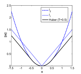
Figure 2: The $l_{1}$, $l_{2}$ and Huber norms. The Huber penalty is a smooth relaxation of the $l_{1}$-norm which acts quadratically for input values smaller than the threshold while it behaves linearly for larger inputs. For inputs with heavy tail behavior, linear penalization in the regularization term is advantageous compared to the quadratic penalty functions in which the cost function becomes dominated by a few large values in the tail of the distribution.

In downscaling of state variables containing frequent jumps and isolated singularities (e.g., local rainfall extremes) using regularization in the derivative space (i.e., $\mathbf{L}\mathbf{x}$ is an approximate derivative measure), the $l_{1}$-like norms typically preserve rapid variations and lead to improved and sharper solutions, compared to the overly smooth results of the $l_{2}$-regularization; see, examples presented by Ebtehaj et al. [2012] for rainfall downscaling and other examples in the next section.

3.2 Statistical Interpretation

From the frequentist statistical point of view, it is easy to show that the WLS solution of (3) is equivalent to the maximum likelihood estimator (ML)

$$\hat{\mathbf{x}}_{ML}=\underset{\mathbf{x}}{{\rm argmax}}\,p\left(\mathbf{y}|\mathbf{x}\right),$$ (9)

given that the likelihood density is Gaussian, $p\left(\mathbf{y}|\mathbf{x}\right)\propto\exp\left(\nicefrac{{-1}}{{2}}(\mathbf{y}-\mathbf{H}\mathbf{x})^{T}\mathbf{R}^{-1}(\mathbf{y}-\mathbf{Hx})\right)$. Specifically, taking $-\log(\cdot)$, one can find the minimizer of the negative log-likelihood function $-\log\left\{p(\mathbf{y}|\mathbf{x})\right\}$ as,

$$\hat{\mathbf{x}}_{ML} = \underset{\mathbf{x}}{{\rm argmin}}\left\{\frac{1}{2}(\mathbf{y}-\mathbf{H}\mathbf{x})^{T}\mathbf{R}^{-1}(\mathbf{y}-\mathbf{Hx})\right\}$$ (10)

$$= \underset{\mathbf{x}}{{\rm argmin}}\left\{\frac{1}{2}\left\|\mathbf{y}-\mathbf{Hx}\right\|_{\mathbf{R}^{-1}}^{2}\right\},$$

which is identical to the WLS solution of (3).

It is important to note that in the ML estimator, $\mathbf{x}$ is considered to be a deterministic variable (fixed) while $\mathbf{y}$ has a random nature.

On the other hand, in the Bayesian perspective, the regularized solution of equation (5) is equivalent to the maximum a posteriori (MAP) estimator

$$\hat{\mathbf{x}}_{MAP}=\underset{\mathbf{x}}{{\rm argmax}}\,p\left(\mathbf{x}|\mathbf{y}\right),$$ (11)

where both $\mathbf{x}$ and $\mathbf{y}$ are considered of random nature. Specifically, using Bayes theorem, ignoring the constant terms in $\mathbf{x}$ and applying $-\log(\cdot)$ on the posterior density $p(\mathbf{x}|\mathbf{y})$, we get

$$\hat{\mathbf{x}}_{MAP} = \underset{\mathbf{x}}{{\rm argmin}}\left\{-\log\,\left(\frac{p(\mathbf{y}|\mathbf{x})\,p(\mathbf{x})}{p(\mathbf{y})}\right)\right\}$$ (12)

$$= \underset{\mathbf{x}}{{\rm argmin}}\left\{-\log\,p\left(\mathbf{y}|\mathbf{x}\right)-\log\,p(\mathbf{x})\right\}.$$

The first term, $-\log\,p\left(\mathbf{y}|\mathbf{x}\right)$, is just the negative log-likelihood as appeared in the ML estimator and the second term is called the prior which accounts for the a priori knowledge about the density of the state vector $\mathbf{x}$. Accordingly, the proposed Tikhonov regularization in (5) is equivalent to the MAP estimator assuming that the state, or the linear transformed state $\mathbf{L}\mathbf{x}$, is a multivariate Gaussian of the form

$$\log\,p(\mathbf{x})\propto\mathbf{x}^{T}\mathbf{Q}\mathbf{x},$$ (13)

where the covariance is $\mathbf{Q}=\mathbf{L}^{T}\mathbf{L}$ [e.g., Tikhonov et al., 1977; Elad and Feuer, 1997; Levy, 2008].

Clearly, the choice of the $l_{1}$-norm in equation (7), implies that $\log\,p(\mathbf{x})\propto\left\|\mathbf{L}\mathbf{x}\right\|_{1}$ or say the transformed state can be well explained by a multivariate Laplace density with heavier tail than the Gaussian case [e.g., Tibshirani, 1996; Lewicki and Sejnowski, 2000]. Similarly, selecting the Huber norm can also be interpreted as $\log\,p(\mathbf{x})\propto\sum_{i}\rho_{T}(x_{i})$, which is equivalent to assuming the Gibbs density function as the prior probability model of the state [Geman and Geman, 1984; Schultz and Stevenson, 1994]. The equivalence between the regularized estimation approach, which imposes constraints on the regularity of the solution, and its Bayesian counterpart, which imposes constraints on the prior probability of the state is very insightful. This relationship establishes an important duality which can guide the selection of regularization depending on the statistical properties of the state in the real or derivative space.

3.3 Examples on Rainfall DS

3.3.1 Problem Formulation and Settings

To downscale a remotely sensed hydrometeorological signal using the explained discrete regularization methods, we need to have proper mathematical models for the downgrading operator and also a priori knowledge about the form of the regularization term. Clearly, the downgrading operator in the presented framework needs to be a linear approximation of the sampling property of the sensor. If a sensor directly measures the state of interest, while its maximum frequency channel is smaller than the maximum frequency content of the state (e.g., precipitation), the result of the sensing would be a smoothed and possibly downsampled version of the true state. Thus, each element of the observed state in a grid-scale might be considered as an average (low-resolution) representation of the true state, lacking the high-resolution subgrid-scale variability. To have a simple and tractable mathematical model, the downgrading matrix might be considered translation invariant and decomposed into $\mathbf{H}=\mathbf{D}\mathbf{C}$, where $\mathbf{C}$ encodes the smoothing effect and $\mathbf{D}$ contains information about the sampling rate of the sensor. As a simple mathematical model, let us suppose that each grid point in the low-resolution observation is a (weighted) average of a finite size neighborhood of the true state, positioned at the center of the grid. In this case, the sensor smoothing property in $\mathbf{C}$ can be encoded by the filtering and convolution operations, while $\mathbf{D}$ acts as a linear downsampling operator (Figure 3). These matrices can be formed explicitly, while direct matrix-vector multiplication (e.g., $\mathbf{C}\mathbf{x}$ and $\mathbf{C}^{T}\mathbf{x}$, $\mathbf{x}\in\mathbb{R}^{m}$), requires a computational cost in the order of $\mathcal{O}(m^{2})$. However, for large scale problems, those matrix-vector multiplications (i.e., convolution operation) are typically performed more efficiently, for instance in the Fourier domain with computational cost of $\mathcal{O}(m\log m)$. Figure 3 sketches the above matrix-vector multiplication via the filtering and convolution operations.

${\rm a)}$

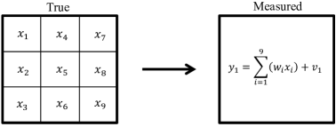
$\overset{{\rm Kernel}}{\begin{bmatrix}c_{1}&c_{4}&c_{7}\\ c_{2}&c_{5}&c_{8}\\ c_{3}&c_{6}&c_{9}\end{bmatrix}}\,\,\,\,\,\overset{{\rm b)\,Filtering}}{\begin{array}[]{c}\hrulefill\hfil\\ \begin{array}[]{ccccc}0&0&0&0&0\\ 0&0&0&0&0\\ 0&0&1&0&0\\ 0&0&0&0&0\\ 0&0&0&0&0\end{array}\xrightarrow{\mathbf{C}}\begin{array}[]{ccccc}0&0&0&0&0\\ 0&c_{9}&c_{6}&c_{3}&0\\ 0&c_{8}&c_{5}&c_{2}&0\\ 0&c_{7}&c_{4}&c_{1}&0\\ 0&0&0&0&0\end{array}\end{array}}\,\,\,\,\,\,\,\,\,\overset{{\rm c)\,Convolution}}{\begin{array}[]{c}\hrulefill\hfil\\ \begin{array}[]{ccccc}0&0&0&0&0\\ 0&0&0&0&0\\ 0&0&1&0&0\\ 0&0&0&0&0\\ 0&0&0&0&0\end{array}\xrightarrow{\mathbf{C}^{T}}\begin{array}[]{ccccc}0&0&0&0&0\\ 0&c_{1}&c_{4}&c_{7}&0\\ 0&c_{2}&c_{5}&c_{8}&0\\ 0&c_{3}&c_{6}&c_{9}&0\\ 0&0&0&0&0\end{array}\end{array}}$

$\,\overset{{\rm d)\,Upsampling\,and}\,{\rm Downsampling}}{\begin{array}[]{c}\hrulefill\hfil\\ \begin{array}[]{ccc}1&1&1\\ 1&1&1\\ 1&1&1\end{array}\begin{array}[]{c}\xrightarrow{\mathbf{D}^{T}}\\ \xleftarrow[\mathbf{D}]{}\end{array}\begin{array}[]{ccccc}1&0&1&0&1\\ 0&0&0&0&0\\ 1&0&1&0&1\\ 0&0&0&0&0\\ 1&0&1&0&1\end{array}\end{array}}$

Figure 3: Two dimensional mathematical models of the smoothing and downsampling property of a low-resolution sensor via the convolution operation. (a) A simple representation of the used observation model for a neighborhood of size 3-by-3 using a simple uniform averaging filter. (b-c) A sample effect of the filtering operation ($\mathbf{C}$) and its transpose ($\mathbf{C}^{T}$) on a discrete 2D unit pulse, given the shown $3\times 3$ kernel. (d) A sample effect of the 2D downsampling operator ($\mathbf{D}$) and its transpose ($\mathbf{D}^{T}$) with scaling ratio 2. In the filtering operation, we basically slide the kernel over the field and sum the element-wise multiplication of the kernel elements with those of the field and then put the results at the center of the current position of the kernel. However, in the convolution operation we first rotate the kernel by $180^{\circ}$ and follow the same procedure.

As is evident, the smoothing kernel needs to be estimated for each sensor, possibly by learning from a library of coincidental high and low-resolution observations (Ebtehaj et al., 2012, e.g.,), or through a direct minimization of an associated cost. In the absence of prior knowledge, one possible choice is to assume that the sensor observes a coarse grained (i.e., non-overlapping box averaging) and noisy version of the true state. In other words, to produce a field at the grid-scale of $s_{c}\times s_{c}$ from a $1\times 1$, this assumption is equivalent to selecting a uniform smoothing kernel of size $s_{c}\times s_{c}$ followed by a downsampling ratio of $s_{c}$ (Figure 4a).

$\begin{array}[]{c}{\rm a)}\\ \\ \\ \\ \end{array}\frac{1}{s_{c}^{2}}\begin{bmatrix}1&\cdots&1\\ \vdots&\ddots&\vdots\\ 1&\cdots&1\end{bmatrix}_{s_{c}\times s_{c}}\,\,\,\,\,\,\,\,\,\,\begin{array}[]{c}{\rm b)}\\ \\ \\ \\ \end{array}\triangledown^{2}=\frac{4}{\left(\kappa+1\right)}\begin{bmatrix}\frac{\kappa}{4}&\frac{1-\kappa}{4}&\frac{\kappa}{4}\\ \frac{1-\kappa}{4}&-1&\frac{1-\kappa}{4}\\ \frac{\kappa}{4}&\frac{1-\kappa}{4}&\frac{\kappa}{4}\end{bmatrix}$

Figure 4: (a) A uniform smoothing (low-pass) kernel of size $s_{c}\times s_{c}$. (b) The discrete (high-pass) generalized Laplacian filter of size $3\times 3$, where $\kappa$ is a parameter ranging between 0 to 1. The Laplacian coefficients, obtained by filtering the 2D state with the Laplacian kernel, are approximate measures of the second order derivative. Throughout this paper, we choose $\kappa=0.5$ which corresponds to the 2D standard second order differencing operation.

The choice of the regularization term also plays a very important role on the accuracy of the DS solution. Figure 5a demonstrates a NEXRAD reflectivity snapshot ($1\times 1$ km) over the Texas TRMM ground validation (GV) site, while Figure 5b displays the standardized histogram of the discrete Laplacian coefficients (second order differences) and the fitted exponential of the form $p(x)\propto\exp\left(-\lambda\left|x\right|\right)$. It is seen that the analyzed rainfall image exhibits a (near) sparse representation in the derivative space with a large mass at zero and heavier tail than the Gaussian. Although not shown here, the universality of this structure can be observed in other rainfall reflectivity fields, denoting that the choice of the $l_{1}$-like regularization is preferred in the rainfall DS problems rather than the choice of the Tikhonov regularization; see, Ebtehaj and Foufoula-Georgiou [2011a] for a thorough survey of rainfall statistics in derivative space, in terms of the wavelet coefficients.

This well behaved non-Gaussian structure in the derivative space mainly arises due to the presence of spatial coherence (correlation) in the rainfall fields and abrupt occurrences of piece-wise discontinuities (large gradients). In effect, over the large areas of uniform rainfall intensity, a measure of derivative translates rainfall values into a large number of (near) zero values; however, over the less frequent jumps and isolated high-intensity rain-cells, values of the derivative measure are markedly larger than zero and form the tails. Note that this non-Gaussianity is due to the intrinsic spatial structure of rainfall reflectivity fields and can not be resolved by a logarithmic or power-law transformation (e.g., $Z$-$R$ relationship). It is easy to see that after applying the $Z$-$R$ relationship on the reflectivity fields, the shape of the rainfall histogram remains non-Gaussian and still can be explained by the Laplace density (not shown here). In practice, the histogram of the derivatives may exhibit a thicker tail than the Laplace density, requiring a heavier tail model such as the Generalized Gaussian Density (GGD) of the form $p(x)\propto\exp\left(-\lambda\left|x\right|^{p}\right)$, where $p<1$ [see, Ebtehaj and Foufoula-Georgiou, 2011a]. However, using such a prior model gives rise to a non-convex optimization problem in which convergence to the global minimum can not be guaranteed. Hence, the choice of the $l_{1}$-norm (the Laplace prior) is indeed the closest convex regularization that can partially fulfill the strict statistical interpretation, while the actual prior might still be better explained by a heavier tail model than the Laplace density.

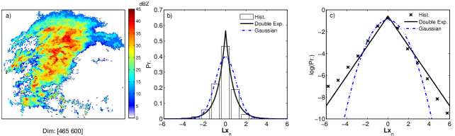
Figure 5: A rainfall reflectivity field and the distribution of its standardized Laplacian coefficients with unit standard deviation, $\mathbf{L}\mathbf{x}_{{\rm n}}=\nicefrac{\mathrm{\mathbf{L}\mathbf{x}}}{\mathrm{std(\mathbf{L}\mathbf{x})}}$, where ${\rm std(\cdot)}$ is the standard deviation operator and $\triangledown^{2}\mathbf{x}=\mathbf{L}\mathbf{x}$. (a) NEXRAD reflectivity snapshot at the TRMM GV-site in Houston, TX (HSTN) on 1998/11/13 (00:02:00 UTC) at scale $1\times 1$ km. (b) The histogram of the standardized Laplacian coefficients , with $\kappa=0.5$ (Figure 4), and (c) the log-histogram. Note that, the zero coefficients over the non-rainy background have been excluded from the histogram analysis. The dash line in (b) is the least squares fitted exponential of the form $p(x)\propto\exp\left(-\lambda\left|x\right|\right)$ and the dash-dot line shows a standard normal distribution for comparison. The log-histogram in (c) contrasts the heavy tailed structure of the coefficients versus the Gaussian distribution clearer than the original histogram in (b).

Following our observations related to the distribution of the rainfall derivatives, here we direct our attention to the Huber penalty function as a smooth approximation of the $l_{1}$-regularization,

$$\mathcal{J}(\mathbf{x})=\frac{1}{2}\left\|\mathbf{y}-\mathbf{Hx}\right\|_{\mathbf{R}^{-1}}^{2}+\lambda\,\left\|\mathbf{L}\mathbf{x}\right\|_{{\rm Hub}}.$$ (14)

Minimization of the above cost function can be easily achieved using first order efficient gradient descent based methods. However, as the rainfall fields are non-negative, we used the gradient projection (GP) method [Bertsekas, 1999, pp. 228], to solve the above problem in a constrained mode such that $\mathbf{x}\succeq 0$ (see Appendix A).

3.3.2 Results

The same rainfall snapshot shown in Figure 5 has been used to examine the performance of the proposed regularized DS methodologies. Throughout the paper, to make the reported parameters independent of the range of intensity values, the rainfall reflectivity fields are first scaled into the range between 0 and 1; however, the results and Figures are presented in the true range.

To demonstrate the performance of the proposed regularized DS methodology, the NEXRAD high-resolution observation $\mathbf{x}$ was assumed as the true state while the low-resolution observations $\mathbf{y}$ were obtained by smoothing $\mathbf{x}$ with an average filter of size $s_{c}\times s_{c}$ followed by a downsampling ratio $s_{c}$. Given the true state and constructed observations, we can quantitatively examine the effectiveness of the presented DS methods. In fact, selecting some common quality metrics, we demonstrate the effective improvement of those measures using the presented regularized DS framework.

Both the Huber and Tikhonov regularizations were examined to downscale the observations from scales $4\times 4$ and $8\times 8$ km down to $1\times 1$ km (Figure 6). A very small amount of white noise (i.e., standard deviation of $1{\rm e}$-3) was added to the low-resolution observations (equation 2), giving rise to a diagonal error covariance matrix. In both of the regularization methods, the regularization parameter $\lambda$ was set to $5{\rm e}$-3 and ${\rm 1e}$-2 for downscaling from 4-to-1 and 8-to-1 km in grid spacing, respectively. These values are selected through trial and error; however, there are some formal methods for automatic estimation of this parameter which are left for future work [e.g., the L-curve; see Hansen, 2010]. In our experiments, it turned out that small values of the Huber threshold $T$, typically less than $10$% of the field maximum range of variability, lead to a successful recovery of isolated singularities and local extreme rainfall cells (Figure 7).

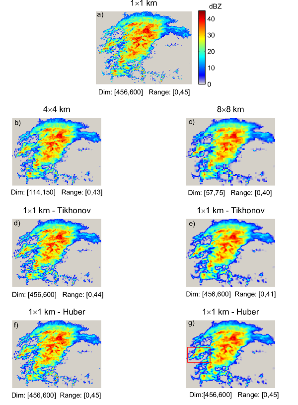
Figure 6: Sample results of the rainfall regularized Downscaling (DS). (a) True high-resolution rainfall reflectivity: NEXRAD snapshot at the TRMM GV-site in Houston, TX (HSTN) on 1998/11/13 (00:02:00 UTC) at resolution $1\times 1$ km. (b-c) The synthetically generated, $4\times 4$ and $8\times 8$ km, coarse-scale and noisy observations of the true rainfall reflectivity field. Left column: Tikhonov (d) and Huber (f) regularization results for downscaling from 4-to-1 km ($T=0.02$). Right column: Tikhonov (e) and Huber (g) regularized DS for downscaling from 8-to-1 km ($T=0.04)$. Zooming views of the delineated box in (g) are shown in Figure 7.

In the studied snapshot, coarse graining of the rainfall reflectivity fields to the scales of $4\times 4$ and $8\times 8$ kilometers was equivalent to loosing almost 20 and 30 percent of the rainfall energy in terms of the relative Root Mean Squared Error (RMSE), ${\rm RMSE}_{{\rm r}}=\nicefrac{{\left\|\mathbf{x}-\hat{\mathbf{x}}\right\|_{2}}}{{\left\|\mathbf{x}\right\|_{2}}}$ (see, Table 1). Note that, to compute the RMSE of the low-resolution observations, the size of those fields was extended to the size of the true field using the nearest neighborhood interpolation, that is, each low-resolution pixel was replaced with $s_{c}\times s_{c}$ pixels with the same intensity value. In addition to the relative RMSE measure, we also used three other metrics: (1) Relative Mean Absolute Error (MAE), ${\rm MAE}_{{\rm r}}=\nicefrac{{\left\|\mathbf{x}-\hat{\mathbf{x}}\right\|_{1}}}{{\left\|\mathbf{x}\right\|_{1}}}$; (2) A logarithmic measure often called the peak signal-to-noise ratio (PSNR), ${\rm PSNR}=20\log_{10}\left(\nicefrac{{\max\left(\hat{\mathbf{x}}\right)}}{{{\rm{\rm std}\left(\mathbf{x}-\hat{\mathbf{x}}\right)}}}\right)$ where ${\rm std}\left(\cdot\right)$ denotes the standard deviation and; (3) The Structural Similarity Index (SSIM) by Wang et al. [2004]. The PSNR in decibel (dB), represents a measure that not only contains RMSE information but also encodes the recovered range. The latter measure varies between -1 and 1 and the upper bound refers to the case where the estimated and reference fields are perfectly matched. The SSIM metric is popular in the image processing community as it takes into account not only the marginal statistics such as the RMSE but also the correlation structure between the estimated and reference (true) image. This metric seems very promising for analyzing the forecast mismatch with observations in hydro-meteorological studies, especially when the systematic errors in the large scale features of the predicted state (e.g., displacement error) might be more dominant than the random errors; see Ebtehaj et al. [2012] for applications of SSIM in rainfall downscaling.

On average, it was seen that one third of the lost relative energy of the rainfall reflectivity fields can be restored via the regularized DS (Table 1). The $l_{2}$-regularization led to smoother results and as the scaling ratio grows, this regularization was almost incapable to recover the peaks and the correct variability range of the rainfall field (Figure 7). Typically, as expected, the Huber regularization results were slightly better than the Tikhonov ones. For large scaling ratios (i.e., > $4\times 4$ km) the results of those methods tended to coincide in terms of the global quality metrics such the RMSE. However, using the Huber prior, the recovered range was markedly better than that by the Tikhonov regularization as reflected in the PSNR metric.

Metric†	Observations		Tikhonov		Huber
	$4\times 4$ km	$8\times 8$ km	$4\times 4$ km	$8\times 8$ km	$4\times 4$ km	$8\times 8$ km
${\rm RMSE}_{{\rm r}}$	0.19	0.29	0.15	0.20	0.14	0.19
${\rm MAE}_{{\rm r}}$	0.15	0.25	0.13	0.18	0.11	0.17
SSIM	0.71	0.56	0.78	0.66	0.80	0.66
PSNR	23.8	19.6	26.5	23.1	27.0	24.0

Table 1: Results showing the effectiveness of the proposed regularized DS by reducing the estimation error and increasing the accuracy of the rainfall fields. The first two columns refer to the values of the quality metrics obtained by comparing the constructed low-resolution observations with true $1\times 1$ km reflectivity field. The performance of the Huber prior is slightly better than the $l_{2}$-regularization, especially for the small scaling ratios (i.e., $\leq 4\times 4$ km).^† ${\rm RMSE}_{r}$: relative root mean squared error; ${\rm MAE}_{r}$ : relative maximum absolute error; SSIM: structural similarity; and PSNR: peak signal to noise ratio.

4 Regularized Data Fusion

4.1 Problem Formulation

Analogous to the DS problem in the previous section, here we focus on the formulation of the DF problem. In the DF class of problems, typically, an improved estimate of the true state is sought from a series of low-resolution and noisy observations. Let $\mathbf{x}\in\mathbb{R}^{m}$ be the true state of interest while a set of $N$ downgraded measurements $\mathbf{y}^{i}\in\mathbb{R}^{n_{i}}$, $i=1,\ldots,\,N$, are available through the following linear observation model

$$\mathbf{y}^{i}=\mathbf{H}^{i}\mathbf{x}+\mathbf{v},$$ (15)

where $n_{i}\ll m$, $\mathbf{H}^{i}\in\mathbb{R}^{n_{i}\times m}$ and $\mathbf{v}^{i}\sim\mathcal{N}\left(0,\,\mathbf{R}^{i}\right)$ denotes uncorrelated Gaussian error in $\mathbb{R}^{n_{i}}$, $\underset{i\neq j}{\mathbb{E}}\left[\mathbf{v}^{i}\left(\mathbf{v}^{j}\right)^{T}\right]=0$. Compared to the DS family of problems, DF is more constrained in the sense that usually there are more equations than the number of unknowns, $\Sigma_{i}^{N}n_{i}\gg m$, giving rise to an overdetermined linear system. As previously explained, naturally the linear weighted least squares (WLS) estimate of the true state, given the series of $N$ observations, amounts to solving the following optimization problem:

$$\hat{\mathbf{x}}=\underset{\mathbf{x}}{{\rm argmin}}\left\{\frac{1}{2}\sum_{i=1}^{N}\left(\left\|\mathbf{y}^{i}-\mathbf{H}^{i}\mathbf{x}\right\|_{\left(\mathbf{R}^{i}\right)^{-1}}^{2}\right)\right\}.$$ (16)

Notice that the solution of the above problem not only contains information about all of the available observations (Fusion) but also, with proper design of the observation operators, allows us to obtain an estimate with higher resolution than any of the available observations (Downscaling). Clearly, the inverse of each covariance matrix in (16) plays the role of the relative contribution or weight of each $\mathbf{y}^{i}$ in the overall cost. In other words, if the elements of covariance matrix of a particular observation vector are large compared to those of the other observation vectors, naturally, the contribution of that observation to the obtained solution would be less significant.

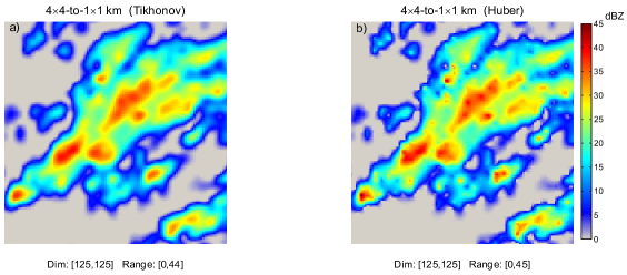
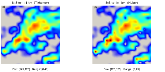
Figure 7: A zooming view for comparing qualitatively the Tikhonov (a, c) versus Huber (b, d) regularization, for the Downscaling (DS) example over the delineated box in Figure 6g. The results indicate a better performance of the Huber regularization, especially for smaller scaling ratios. The Huber regularization yields sharper results and is more capable to recover high-intensity rainfall cells and the correct range of variability; see Table 1 for quantitative comparison using a suit of metrics.

For notational convenience, the above system of equations can be augmented as follows:

$$\begin{bmatrix}\mathbf{y}^{1}\\ \vdots\\ \mathbf{y}^{N}\end{bmatrix} = \begin{bmatrix}\mathbf{H}^{1}\\ \vdots\\ \mathbf{H}^{N}\end{bmatrix}\mathbf{x}+\begin{bmatrix}\mathbf{v}^{1}\\ \vdots\\ \mathbf{v}^{N}\end{bmatrix}$$

$$\Rightarrow\underline{\mathbf{y}} = \underline{\mathbf{H}}\mathbf{x}+\underline{\mathbf{v}}$$ (17)

where, the concatenated error vector $\underline{\mathbf{v}}$ has the following block diagonal covariance matrix,

$$\mathbf{\underline{R}}=\mathbb{E}\left[\mathbf{\underline{\mathbf{v}}}\mathbf{\underline{\mathbf{v}}}^{T}\right]=\begin{bmatrix}\mathbf{R}^{1}&&0\\ &\ddots\\ 0&&\mathbf{R}^{N}\end{bmatrix}.$$ (18)

Therefore, the DF problem can be recast as the classic problem of estimating the true state from the augmented observation model of $\underline{\mathbf{y}}=\underline{\mathbf{H}}\mathbf{x}+\underline{\mathbf{v}}$. Setting the gradient of the cost function in equation (16) to zero, yields the following linear system:

$$\left(\underline{\mathbf{H}}^{T}\mathbf{\underline{R}}^{-1}\mathbf{\underline{H}}\right)\hat{\mathbf{x}}=\mathbf{\underline{H}}^{T}\mathbf{\underline{R}}^{-1}\mathbf{\underline{y}}.$$ (19)

In this case, the left hand side $\underline{\mathbf{H}}^{T}\mathbf{\underline{R}}^{-1}\mathbf{\underline{H}}$ is likely to be very ill-conditioned giving rise to an unstable LS solution, highly sensitive to any perturbation in the observation vector in the right-hand side (Figure 8c) [see, e.g., Elad and Feuer, 1997; Hansen, 2010].

One possible remedy for stabilizing the solution is regularization. Recalling the formulation discussed in the previous section, a general regularized form of the DF problem can be written as

$$\hat{\mathbf{x}}=\underset{\mathbf{x}}{{\rm argmin}}\left\{\frac{1}{2}\left\|\mathbf{\underline{y}}-\underline{\mathbf{H}}\mathbf{x}\right\|_{\mathbf{\underline{R}}^{-1}}^{2}+\lambda\,\psi_{\mathbf{L}}\left(\mathbf{x}\right)\right\},$$ (20)

where the convex function $\psi_{\mathbf{L}}\left(\mathbf{x}\right)$ can take different penalty norms such as: the smooth Tikhonov $\left\|\mathbf{L}\mathbf{x}\right\|_{2}^{2}$; the non-smooth $l_{1}$-norm $\left\|\mathbf{L}\mathbf{x}\right\|_{1}$; and the smooth Huber-norm $\left\|\mathbf{L}\mathbf{x}\right\|_{{\rm Hub}}$.

For the case of the linear Tikhonov regularization, computation of the solution requires to invert the Hessian ($\mathbf{\underline{H}}^{T}\mathbf{\underline{R}}^{-1}\mathbf{\underline{H}}+2\lambda\,\mathbf{L}^{T}\mathbf{L}$) of the objective function similar to equation (6). Analogous to the DS problem, the covariance of the posterior distribution is $\left(\mathbf{\underline{H}}^{T}\mathbf{\underline{R}}^{-1}\mathbf{\underline{H}}+2\lambda\,\mathbf{L}^{T}\mathbf{L}\right)^{-1}$.

Based on the selected type of regularization, statistical interpretation of the DF regularized class of problems is also similar to what was explained in Section 3.2. In other words, given the augmented classic observation model in (17), it is easy to see that the solution of (16) is the ML estimator while (20) can be interpreted as the MAP estimator with a prior density depending on the form of the regularization term.

4.2 Example on Rainfall DF

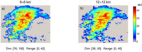
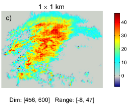
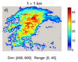
Figure 8: Data Fusion and Downscaling of multi-sensor remotely sensed rainfall reflectivity fields using the Huber regularization. (a-b) Reconstructed low-resolution and noisy rainfall observations at scale $6$ and $12$ km in grid spacing. (c) The results of the WLS solution in (16), and (d) the solution of Huber regularized DF with $\lambda=1{\rm e}$-3 and $T=1{\rm e}$-2.

To quantitatively analyze the effectiveness of the regularized DF for rainfall data, we reconstructed two synthetic low-resolution and noisy observations from the original high-resolution NEXRAD reflectivity snapshot. To resemble different sensor constraints we chose different smoothing and downsampling operations for each of the reconstructed field. The first observation field $\mathbf{y}_{1}$ was produced, at resolution $6\times 6$ km, using a simple averaging filter of size $6\times 6$ followed by a downsampling ratio of $s_{c}=6$. Analogously, the second field $\mathbf{y}_{2}$ was generated at scale $12\times 12$ km using a Gaussian smoothing kernel of size the $12\times 12$ with a standard deviation of $4$. A white Gaussian noise, with standard deviation of $1{\rm e}$-2 and $2{\rm e}$-2 was also added, respectively, to resemble the measurement random error. Roughly speaking, this selection of the error magnitudes implies that the degree of confidence (relative weight) on the observation at $6\times 6$ km is twice as large as for the one at $12\times 12$ km scale. According to the selected smoothing and downsampling operations, the downgrading operators $\mathbf{H}^{1}$ and $\mathbf{H}^{2}$ are designed to produce a high-resolution field at the scale of $1\times 1$ km. To solve the DF problem, we have used the same settings for the Gradient Projection (GP) method as explained in Appendix A.

The solution of the ill-conditioned WLS formulation or the ML estimator in (16) is blocky, out of range and severely affected by the amplified inverted noise (Figure 8c). On the other hand, the Huber regularization can properly restore a fine-scale and coherent estimate of the rainfall field. The results show that almost 30% of the uncaptured subgrid energy of the rainfall field can be restored through solving the regularized DF problem (Table 2). Improvements of the selected fidelity measures in the DF problem is more pronounced than the results of the DS experiment. This naturally arises, because more observations are available in the DF problem than the DS one and thus, the results are likely to be more accurate.

Metric	Observations		DF results
	$6\times 6$ km	$12\times 12$ km	$1\times 1$ km
${\rm RMSE}_{{\rm r}}$	0.25	0.35	0.17
${\rm MAE}_{{\rm r}}$	0.21	0.32	0.15
SSIM	0.60	0.50	0.72
PSNR	21.3	18.1	25.0

Table 2: Values of the selected fidelity metrics in the rainfall DF experiment using the Huber regularization, see the text for the definitions. Here, metrics refer to comparison of the low-resolution ($6\times 6$ and $12\times 12$ km) observations the DF results with the true field ($1\times 1$ km).

5 Regularized Variational Data Assimilation

5.1 Problem Formulation

Compared to the previously explained problems of downscaling and data fusion, the data assimilation (DA) problem is more involved in the sense that we need to address the evolution of a dynamical system and the available (low-resolution) observations at the same time in the estimation process. Despite the increased complexity, DA shares the same principles with the explained formulations of the DS and DF problems, from the estimation point of view. Here, we briefly explain the linear 3D and 4D-VAR data assimilation schemes and extend their formulations to a regularized format. Sample results of the regularized variational data assimilation problem are illustrated on the estimation of the initial conditions of the linear heat equation in a 3D-VAR setting.

The 3D-VAR is a memoryless assimilation method. In other words, at each time step, the best estimate of the true state or say analysis is obtained based only on the present-time noisy observations and background information of the dynamical system. The analysis is then being used for forecasting the state at the next time step an so on. Suppose that the true state of interest at discrete time $t_{k}$ is denoted by $\mathbf{x}_{k}\in\mathbb{R}^{m}$, a single noisy observation is $\mathbf{y}_{k}\in\mathbb{R}^{n}$, and $\mathbf{x}_{k}^{b}\in\mathbb{R}^{m}$ represents the background state. In the linear 3D-VAR data assimilation problem, obtaining the analysis state $\mathbf{x}_{k}^{a}\in\mathbb{R}^{m}$ amounts to finding the minimum point of the following cost function:

$$\mathcal{J}_{3D}(\mathbf{x}_{k})=\frac{1}{2}\left\|\mathbf{x}_{k}^{b}-\mathbf{x}_{k}\right\|_{\mathbf{B}^{-1}}^{2}+\frac{1}{2}\left\|\mathbf{y}_{k}-\mathbf{H}\mathbf{x}_{k}\right\|_{\mathbf{R}^{-1}}^{2}.$$ (21)

In equation (21), $\mathbf{B}\in\mathbb{R}^{m\times m}$ is the background error covariance matrix, $\mathbf{H}$ denotes the observation operator, while the analysis is the optimal solution: $\mathbf{x}_{k}^{a}={\rm\underset{\mathbf{x}_{k}}{argmin}}\left\{\mathcal{J}_{3D}(\mathbf{x}_{k})\right\}$. Here we assume that the observation matrix is translation invariant. Clearly, this 3D-VAR problem is the WLS problem which has the following analytic solution

$$\mathbf{x}_{k}^{a}=\left(\mathbf{B}^{-1}+\mathbf{H}^{T}\mathbf{R}^{-1}\mathbf{H}\right)^{-1}\left(\mathbf{B}^{-1}\mathbf{x}_{k}^{b}+\mathbf{H}^{T}\mathbf{R}^{-1}\mathbf{y}_{k}\right).$$ (22)

Because the error covariance matrices are positive definite, the matrix $\mathbf{B}^{-1}+\mathbf{H}^{T}\mathbf{R}^{-1}\mathbf{H}$ is always positive definite and hence invertible. Thus, solution of the 3D-VAR requires no rank or dimension assumption on $\mathbf{H}$. However, this problem might be very ill-conditioned depending on the architecture of the covariance matrices and the measurement operator.

The classic 4D-VAR is, indeed, an extension to the explained 3D-VAR which exploits the temporal memory of the system by constraining the solution (analysis) to the underlying dynamics. Assuming that we are interested in estimating the initial condition of a dynamical model at previous discrete time $t_{k}$, to be used for an improved forecast in future time. The 4D-VAR assimilation method is formulated in such a way that uses the initial background state $\mathbf{x}_{k}^{b}$ and also the observations within a finite discrete time interval $[t_{k},\ldots,\,t_{k+T}]$. Accordingly, this assimilation method amounts to obtaining the minimum point of the following cost function:

$$\mathcal{J}_{4D}(\mathbf{x}_{k})=\frac{1}{2}\left\|\mathbf{x}_{k}^{b}-\mathbf{x}_{k}\right\|_{\mathbf{B}^{-1}}^{2}+\frac{1}{2}\sum_{i=k}^{k+T}\left(\left\|\mathbf{y}_{i}-\mathbf{H}\mathbf{x}_{i}\right\|_{\mathbf{R}_{i}^{-1}}^{2}\right),$$ (23)

while constraining the solution to the underlying dynamics by assuming that $\mathbf{x}_{i}=\mathbf{M}_{k,i}\,\mathbf{x}_{k}$, where $t_{i}\geq t_{k}$. The model operator $\mathbf{M}_{k,i}$ is a discrete linear representation of the system dynamics that evolves the state from $t_{k}$ to $t_{i}$ [e.g., Courtier and Talagrand, 1990; Daley, 1993; Zupanski, 1993; Kalnay, 2003]. Note that, in the above formulation it is implicitly assumed that the background and all measurement errors are mutually uncorrelated. Clearly, the linear 4D-VAR optimization contains a background cost which measures the weighted Euclidean distance of the true initial condition to the background state at the beginning of the interval and an accumulated cost, associated with all of the noisy observations within the selected time interval. Taking into account the imposed constraint by the model operator, the 4D-VAR cost function can be recast as,

$$\mathcal{J}_{4D}(\mathbf{x}_{k})=\frac{1}{2}\left\|\mathbf{x}_{k}^{b}-\mathbf{x}_{k}\right\|_{\mathbf{B}^{-1}}^{2}+\frac{1}{2}\sum_{i=k}^{K+T}\left(\left\|\mathbf{y}_{i}-\mathbf{H}\mathbf{M}_{k,\,i}\,\mathbf{x}_{k}\right\|_{\mathbf{R}_{i}^{-1}}^{2}\right),$$ (24)

where its optimal solution, $\mathbf{x}_{k}^{a}={\rm\underset{\mathbf{x}_{k}}{argmin}}\left\{\mathcal{J}_{4D}(\mathbf{x}_{k})\right\}$, is the analysis state at $k^{th}$ time-step. Thus, it is easy to see that, the linear 3D and 4D-VAR problems are in the category of the classic WLS problems which might be very ill-conditioned.

Analogous to the previous discussions, the generic regularized form of the linear 3D-VAR under the predetermined $\mathbf{L}$-transformation might be considered as follows:

$$\mathbf{x}_{k}^{a}=\underset{\mathbf{x}_{k}}{{\rm argmin}}\left\{\mathcal{J}_{3D}(\mathbf{x}_{k})+\lambda\,\psi_{\mathbf{L}}\left(\mathbf{x}_{k}\right)\right\},$$ (25)

where $\psi_{\mathbf{L}}\left(\mathbf{x}\right)$ can take any of the explained regularization penalty functions including: the smooth Tikhonov $\left\|\mathbf{L}\mathbf{x}\right\|_{2}^{2}$; the non-smooth $l_{1}$-norm $\left\|\mathbf{L}\mathbf{x}\right\|_{1}$; and the smooth Huber-norm $\left\|\mathbf{L}\mathbf{x}\right\|_{{\rm Hub}}$. It is easy to realize that the regularized 4D-VAR estimation of the the initial condition can also take the following form:

$$\mathbf{x}_{k}^{a}=\underset{\mathbf{x}_{k}}{{\rm argmin}}\left\{\mathcal{J}_{4D}(\mathbf{x}_{k})+\lambda\,\psi_{\mathbf{L}}\left(\mathbf{x}_{k}\right)\right\}.$$ (26)

In the above regularized formulations, the solution not only becomes close to the background and observations, in the weighted Euclidean sense, but it is also enforced to follow a regularity imposed by the $\psi_{\mathbf{L}}\left(\mathbf{x}\right)$. Here, we emphasize that the regularization typically yields a stable and improved solution with less uncertainty; however, this gain comes at the price of introducing bias in the solution whose magnitude can be kept small, by proper selection of the regularizer [Hansen, 2010].

5.2 Statistical Interpretation

Statistical interpretation of the classic variational DA problems is a bit tricky compared to the DS and DF class of problems, mainly because of the involvement of the background information in the cost function. Lorenc [1986] derived the 3D-VAR cost function using Bayes theorem and called it the ML estimator [see, e.g., Lorenc, 1988; Bouttier and Courtier, 2002]. More recently, it has been argued that the 4D-VAR, and thus as a special case the 3D-VAR cost function, can be interpreted via the Bayesian MAP estimator [Johnson et al., 2005; Freitag et al., 2010; Nichols, 2010]. For notational convenience, here we only explain the statistical interpretation of the 3D-VAR and its regularized version which can be easily generalized for the case of the 4D-VAR problem.

As discussed earlier, the ML estimator is basically a frequentist view to estimate the most likely value of an unknown deterministic variable from an (indirect) observation with random nature. The ML estimator intuitively requires to find the state that maximizes the likelihood function as $\hat{\mathbf{x}}_{ML}={\rm\underset{\mathbf{x}}{argmax}}\,p\left(\mathbf{y}|\mathbf{x}\right)$. Let us assume that, at time step $t_{k}$, the background $\mathbf{x}_{k}^{b}$ is just a (random) realization of the true deterministic state $\mathbf{x}_{k}$. In other words, we consider $\mathbf{x}_{k}^{b}=\mathbf{x}_{k}+\mathbf{w}$, where the error $\mathbf{w}$ can be well explained by a zero mean Gaussian density $\mathcal{N}\left(0,\,\mathbf{B}\right)$, uncorrelated with the observation error, $\mathbb{E}\left[\mathbf{w}\mathbf{v}^{T}\right]=0$. Here, the background state is treated similar to an observation with random nature. Thus, let us recast the problem of obtaining the analysis as a classic linear inverse problem by augmenting the available information in the from of $\underline{\mathbf{y}}=\underline{\mathbf{H}}\mathbf{x}_{k}+\mathbf{\underline{v}}$, where $\underline{\mathbf{y}}=\left[\left(\mathbf{x}_{k}^{b}\right)^{T},\,\mathbf{y}_{k}^{T}\right]^{T}$ , $\underline{\mathbf{H}}=\left[\mathbf{I},\,\mathbf{H}^{T}\right]^{T}$, and $\underline{\mathbf{v}}\sim\mathcal{N}\left(0,\,\mathbf{\underline{R}}\right)$ with the following block diagonal covariance matrix

$$\underline{\mathbf{R}}=\begin{bmatrix}\mathbf{B}&0\\ 0&\mathbf{R}\end{bmatrix}.$$ (27)

Notice that $\mathbf{\underline{R}}$ is block diagonal because the background and observation errors are uncorrelated. Following the augmented representation and applying $-\log\left(\cdot\right)$, we have $-\log\,p(\mathbf{\underline{y}}|\mathbf{x}_{k})\propto\nicefrac{{1}}{{2}}(\mathbf{\underline{y}}-\mathbf{\underline{H}}\mathbf{x}_{k})^{T}\mathbf{\underline{R}}^{-1}(\underline{\mathbf{y}}-\mathbf{\underline{H}x}_{k})$ and thus it is easy to see that the ML estimator in terms of the augmented observations, $\mathbf{x}_{k}^{a}={\rm\underset{\mathbf{x}_{k}}{argmax}}\,p\left(\mathbf{\underline{y}}|\mathbf{x}_{k}\right)$, is equivalent to minimizing the 3D-VAR cost function in (21). Therefore, following this statistical interpretation, the classic 3D-VAR, can be derived via the frequentist ML estimator.

On the other hand, from the Bayesian perspective, the state of interest and the available observations are considered to be random and the MAP estimator is the optimal point which maximizes the posterior density as $\hat{\mathbf{x}}_{MAP}={\rm\underset{\mathbf{x}}{argmax}}\,p\left(\mathbf{x}|\mathbf{y}\right)$. Let us assume a priori that the (random) state of interest has a Gaussian density with the mean $\mathbf{x}_{b}$ and covariance $\mathbf{B}$, that is $p(\mathbf{x}_{k})\sim\mathcal{N}(\mathbf{x}_{k}^{b},\,\mathbf{B})$. More formally, this assumption implies that the deterministic background is the central (mean) forecast and is related to the random true state via $\mathbf{x}_{k}=\mathbf{x}_{k}^{b}+\mathbf{w}$, where $\mathbf{w}\sim\mathcal{N}\left(0,\,\mathbf{B}\right)$. Therefore, using Bayes theorem; see equation (12), it immediately follows that the 3D-VAR is the MAP estimator with the assumed Gaussian prior for the true state, $\mathbf{x}_{k}^{a}={\rm\underset{\mathbf{x}_{k}}{argmax}}\,p\left(\mathbf{x}_{k}|\mathbf{y}\right)$.

In conclusion, the regularized 3D-VAR in (25) might be interpreted as the MAP estimator, $\mathbf{x}_{k}^{a}={\rm\underset{\mathbf{x}_{k}}{argmax}}\,p\left(\mathbf{x}_{k}|\mathbf{\underline{y}}\right)$, with the prior density, $p(\mathbf{x}_{k})\propto\lambda\,\psi_{\mathbf{L}}\left(\mathbf{x}_{k}\right)$, when we follow the frequentist approach and use the augmented notation to interpret the classic 3D-VAR as the ML estimator. On the other hand, taking the MAP interpretation for the classic 3D-VAR, the regularized version might be understood as the MAP estimator which also accounts for an extra and independent prior on the distribution of the state under the $\mathbf{L}$ transformation.

5.3 Heat Equation Example

The promise of the proposed regularized 3D-VAR data assimilation methodology, is shown via assimilating noisy observations into the dynamics of heat equation with top-hat initial condition. Specifically, we constructed noisy background and noisy-low-resolution observations of the top-hat initial condition and then demonstrated the effectiveness of a proper regularization on the quality of the obtained analysis and forecast states. In the assimilation cycle, we obtained the analyses using the classic and regularized 3D-VAR assimilation methods and then, we examined those analysis states to obtain the forecast state at the next time step. Then the computed analysis and forecast states are compared with their available ground-truth counterparts. Although the heat equation has a diffusive nature and is not sensitive to its initial condition, the provided examples are very illustrative about the role of regularization on the quality of solutions.

For a space-time representation of a 1D scalar quantity $x\left(s,\,t\right)$, the well-known heat equation is

$$\frac{\partial x(s,\,t)}{\partial t} = \gamma\nabla^{2}x(s,\,t)$$ (28)

$$x(s,\,0) = x_{0}(s),$$

where $\infty<s<\infty,\,\,0<t<\infty$. For mathematical treatment, let us assume that $\gamma=1\,\left[\nicefrac{\mathrm{{\rm L}^{2}}}{\mathrm{T}}\right]$. It is well understood that the general solution of the heat equation at time $t$ is then given by the convolution of the initial condition with the fundamental solution (kernel) as

$$x(s,\,t)=\int K\left(s-r,\,t\right)\,x_{0}(r)\,dr,$$ (29)

where

$$K(s,\,t)=(4\pi t)^{-m/2}\exp\left(\frac{-\left|s\right|^{2}}{4t}\right).$$ (30)

We can see that $x\left(s,\,t\right)$ is obtained via convolution of the initial condition by a Gaussian kernel with the standard deviation of $\sigma=\sqrt{2t}$. Clearly, estimation of the initial condition $x_{0}(s)$ only from the diffused and possibly noisy observations $x(s,\,t)$ is an ill-posed deconvolution problem (see equation 1).

To reconstruct a 3D-VAR assimilation experiment, we assume that the true initial condition in discrete space is a vector with 256-elements ($\mathbf{x}\in\mathbb{R}^{m}$ where $m=256$) as follows:

$$\mathbf{x}_{0}=\begin{cases}2&\,\,112\leq x_{i}\leq 144\\ 1&{\rm\,\,\,\,\,\,otherwise},\end{cases}$$ (31)

the so-called top-hat initial condition. We added a white Gaussian noise with $\sigma_{w}=0.05$ to the true initial condition for reconstructing the background state $\mathbf{x}_{0}^{b}$ for the assimilation experiment.

We assumed that the observation vector is a downgraded version of the true state, while the sensor can only capture the mean of every four neighbor elements of the true state. In other words, the observation is a noisy and low-resolution version of the true state with one quarter of its size (Figure 9). To this end, using the linear model in (2), we employed the following architecture for the observation operator:

$$\mathbf{H}=\frac{1}{4}\begin{bmatrix}1\,1\,1\,1&0\,0\,0\,0&\cdots&0\,0\,0\,0\\ 0\,0\,0\,0&1\,1\,1\,1&\cdots&0\,0\,0\,0\\ \vdots&\vdots&\vdots&\vdots\\ 0\,0\,0\,0&0\,0\,0\,0&\cdots&1\,1\,1\,1\end{bmatrix}\in\mathbb{R}^{n\times m},$$ (32)

and an $n$-element white Gaussian observation error with $\sigma_{v}=0.03$, where $n=64$.

The top-hat initial condition is selected to emphasize the role of regularization, especially those with linear penalization (i.e., the Huber or $l_{1}$-norm ). Clearly, the first order derivative of the above initial condition is very sparse. In other words, the first order derivative is zero everywhere on its domain except at the location of the two jumps, resembling a heavy-tailed and sparse statistical distribution. This underlying structure prompts us to use the $l_{1}$-like regularization and first order differencing operator for the $\mathbf{L}$-transform in (25), as follows:

$$\mathbf{L}=\begin{bmatrix}\begin{array}[]{rrrrrr}-1&1&0&\cdots&0&0\\ 0&-1&1&\cdots&0&0\\ \vdots&\vdots&\vdots&\vdots&\vdots&\vdots\\ 0&0&0&\cdots&-1&1\end{array}\end{bmatrix}\in\mathbb{R}^{(m-1)\times m}.$$ (33)

Note that, instead of incorporating a measure of curvature in the regularization term to impose smoothness on the solution, here we seek a solution with minimize total variation.

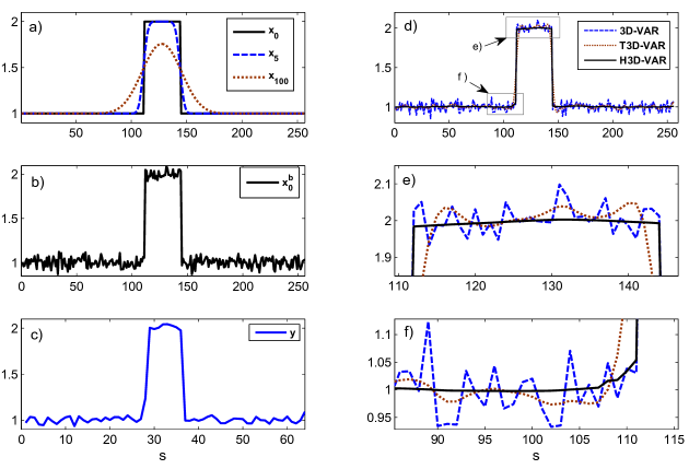
Figure 9: (a) The true initial condition $\mathbf{x}_{0}$ and the results of the heat equation at $t=5$ and 100 $[{\rm T}]$, obtained from convolution of the initial condition with the fundamental Gaussian kernel. (b) The reconstructed background state by adding a white noise with $\sigma_{w}=0.05$. (c) The low-resolution and noisy observation with $\sigma_{v}=0.03$. (d) The results of the classic 3D-VAR and the regularized version using the Tikhonov (T3D-VAR) and the Huber (H3D-VAR) regularizations (see equation 25). (e-f) Magnified parts of of the graphs in (d) over the shown zooming windows.

Figure 9 shows the inputs of the assimilation experiment (left panels) and the results of the analysis cycle (right panels) using the classic versus the regularized 3D-VAR estimators. In this example, it is clear that the classic solution overfits, while slightly damps the noise. Indeed, the 3D-VAR is unable to effectively damp the high-frequency error components and impose the underlying regularity of the true state, because, its cost function is only about minimizing the weighted squared error. On the other hand, in the regularized assimilation methods not only the error term, but also a cost associated with the state regularity is also minimized. The Tikhonov regularization (T3D-VAR), i.e.,$\psi_{\mathbf{L}}\left(\mathbf{x}\right)=\left\|\mathbf{Lx}\right\|_{2}^{2}$ led to a smoother result compared to the classic one with slightly better error statistics. However, result of the Huber regularization (H3D-VAR), i.e., $\psi_{\mathbf{L}}\left(\mathbf{x}\right)=\left\|\mathbf{Lx}\right\|_{{\rm Hub}}$, is the best. The rapidly varying noisy components are effectively damped in this regularization, while the sharp jump discontinuities have been preserved better than the T3D-VAR. The quantitative metrics in Table 3, indicate that in the analysis cycle, the RMSE and MAE metrics are improved dramatically, up to 85% in the H3D-VAR scheme.

Cycle	RMSE			MAE
	3D-VAR	T3D-VAR	H3D-VAR	3D-VAR	T3D-VAR	H3D-VAR
A	0.0475	0.0397	0.0067	0.0376	0.0317	0.0043
F	0.0090	0.0088	0.0043	0.0071	0.0070	0.0033

Table 3: The root mean squared error (RMSE) and the mean absolute error (MAE) for the studied classic and regularized 3D-VAR in the analysis cycle (A) and forecast step (F) .

As previously explained, there is no unique and universally accepted methodology for automated selection of the regularization parameters, namely $\lambda$ and $T$. Here, to select the best parameters in the above assimilation examples, we performed a few trial and error experiments. In other words, over a feasible range of parameter values, we computed the solutions of the regularized assimilation methods and obtained the RMSE measure by comparing those solutions with the true initial condition $\mathbf{x}_{0}$. Figure 10 shows the RMSE for different choices of regularization parameters in both T3D-VAR and H3D-VAR. Note that, the true initial condition is definitely not available in practice; however, here we picked the optimal values of the regularization parameters in the RMSE sense for comparison purposes and demonstrating the importance of a proper regularization. In the T3D-VAR, as expected, larger values of $\lambda$ typically damp rapidly varying error components of the noisy background and observation; however, they may give rise to an overly smooth solution with larger bias and RMSE (Figure 10a). Here, for the T3D-VAR experiment, we picked the value $\lambda_{T}=0.05$ associated with the minimum RMSE (Figure 9). In the H3D-VAR, in addition to the regularizer $\lambda_{H}$, we also need to choose the optimal thresholding value $T$ of the Huber-norm. A contour plot of the RMSE values for different choices of $\lambda_{H}$ and $T$ is shown in Figure 10b. By inspection, we roughly picked $\lambda_{H}=$35 and $T=1.5{\rm e}$-3 for the H3D-VAR assimilation experiment presented in Figure 9.

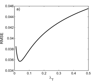
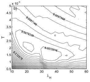
Figure 10: (a) Root mean squared error (RMSE) of the implemented T3D-VAR as a function of the regularizer $\lambda_{T}$. (b) RMSE surface for the H3D-VAR experiment with different choices of the regularizer$\lambda_{H}$ and the threshold value $T$ of the Huber-norm. Clearly, depending on the choice of the regularization method, the strength of the regularizer (magnitude of $\lambda$) might be markedly different.

The main purpose of the DA process is, indeed, to increase the quality of the forecast. Given the initial-time analysis state, we can forecast the profile of the scalar quantity, $x\left(s,\,t\right)$, at any future time step through the heat equation. One important property of the heat equation is its diffusivity. In other words, naturally, noisy components and rapidly varying perturbations are damped but become more correlated as the profile of the initial condition evolves. Thus, rapidly-varying uncorrelated error components become low-varying and correlated features which their detection and removal are naturally more difficult than the uncorrelated ones. Figure 11a, shows the forecast profile at $t=10\,\left[{\rm T}\right]$, obtained by convolution of the initial profile with a Gaussian kernel having standard deviation of $\sigma=\sqrt{2\times 10}$. The results indicate the importance of using a proper regularization on the quality of the forecast in the simple heat equation. The forecasts based on the classic 3D-VAR and the T3D-VAR almost coincide while the regularized result is marginally better. This behavior arises because neither of those methods could properly eliminate the noisy features in the analysis cycle and hence low-varying error components are appeared in the forecast profile. However, the quality metrics in Table 3 indicate that using the H3D-VAR, the RMSE and MAE of the forecast are almost improved more than 50% compared to the other methods.

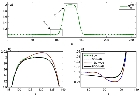
Figure 11: (a) True forecast based on temporal evolution of the top-hat initial condition, Figure 9a, under the heat equation at $t=10\,\left[{\rm T}\right]$. (b-c) Magnified windows showing the forecast quality using different 3D-VAR assimilation methods. Ineffective error removal by the classic 3D and T3D-VAR at the analysis cycle produced large-scale correlated error in the forecast profile, while this problem is less substantial in the result of the H3D-VAR (see, Table 3).

6 Conclusion

In this paper, we presented a new direction in approaching hydrometeorological estimation problems by taking into account important continuity and statistical properties of the underlying states such as the presence of sharp jumps, isolated singularities (i.e., local extremes) and statistical sparsity in the derivative space. We started by explaining the concept of regularization and discussed about the common points of the hydrometeorological problems of downscaling (DS), data fusion (DF), and data assimilation (DA) as discrete linear inverse problems. We argued about the importance of proper regularization which not only makes an inverse problem well-posed but also imposes the desired regularity and statistical property on the solution. Regularization methods were theoretically linked to the underlying statistical structure of the states and it was shown how the statistical information about the density of the state, or its derivative, can be used for proper selection of the regularization method. Specifically, we emphasized three types of regularization, namely, the Tikhonov, $l_{1}$-norm and Huber regularizations. We theoretically showed that these methods are statistically equivalent to the maximum a posteriori (MAP) estimator while respectively assuming the Gaussian, Laplace and Gibbs prior density for the state. It was argued that piece-wise continuity of the state and the presence of frequent jumps are often translated into heavy-tailed distributions in the derivative space that favor the use of $l_{1}$-regularization.

Informed by the non-Gaussian distribution of rainfall derivatives, the effectiveness of the regularized DS and DF problems was tested via analysis of remotely sensed precipitation fields. Then the performance of the regularized DA was studied via assimilating noisy observations into evolution of the heat equation. We showed that regularized assimilation methods outperform the classic 3D-VAR method, especially for the case where the initial condition exhibits a sparse distribution in the derivative space (e.g., first order derivative of the top-hat initial condition).

The presented frameworks can be potentially applied to other hydrometeorological problems, such as soil moisture downscaling and fusion. Clearly, proper selection of the regularization method requires careful statistical analysis of the underlying state of interest. Moreover, the problem of rainfall or soil moisture retrieval from satellite microwave radiance, can be considered as a non-linear inverse problem. This nonlinear inversion may be cast in the presented context, provided that the nonlinear kernel can be (locally) linearized with sufficient accuracy. Application of regularization in the DA problems is in its infancy [e.g.; see, Freitag et al., 2012, for a recent study] and is expected to play significant role over the next decades, especially for highly non-linear chaotic dynamical systems with frequent jumps.

Appendix

Appendix A Gradient Projection for Huber regularization

Here, we present the gradient project (GP) method, using the Huber regularization, only for the downscaling (DS) problem, which can be easily generalized to the data fusion (DF) and data assimilation (DA) cases. In case of the DS problem, the cost function and gradient of the Huber regularization with respect to the elements of the downscaled field are

$$\mathcal{J}(\mathbf{x})=\frac{1}{2}\left\|\mathbf{y}-\mathbf{Hx}\right\|_{\mathbf{R}^{-1}}^{2}+\lambda\,\left\|\mathbf{L}\mathbf{x}\right\|_{{\rm Hub}}$$ (A.1)

$$\nabla\mathcal{J}(\mathbf{x})=\mathbf{H}^{T}\mathbf{R}^{-1}\left(\mathbf{y}-\mathbf{H}\mathbf{x}\right)+\lambda\mathbf{L}^{T}\rho_{T}^{\prime}\left(\mathbf{Lx}\right),$$ (A.2)

where

$$\rho_{T}^{\prime}\left(x\right)=\begin{cases}2x&\left|x\right|\leq T\\ 2T{\rm sign}(x),&\left|x\right|>T.\end{cases}$$ (A.3)

As is evident, the cost function in (A.1), is a smooth and convex function. Thus its minimum can be easily obtained using efficient first order gradient descent methods in large dimensional problems. However, rainfall is a positive process and in order to obtain a feasible downscaled field $\hat{\mathbf{x}}$, the regularized DS problem needs to be solved on the non-negative orthant $\{\mathbf{x}|\,\,x_{i}\geq 0\,\,\forall\,i=1,\ldots,m\}$,

$$\hat{\mathbf{x}} = {\rm argmin}\,\left\{\mathcal{J}(\mathbf{x})\right\}$$ (A.4)

$$\,\,{\rm s.t.\,\,\mathbf{x}\succeq 0}.$$

We have used one of the primitive gradient projection (GP) methods to solve the above constrained DS problem [see, Bertsekas, 1999, pp. 228]. Accordingly, to obtain the solution of (A.4), it amounts to obtaining the fixed point of

$$\mathbf{x}_{*}=\left[\mathbf{x}_{*}-\alpha\nabla\mathcal{J}(\mathbf{x}_{*})\right]^{+},$$ (A.5)

where $\alpha$ is a stepsize and

$$\left[x\right]^{+}=\begin{cases}0&\,\,{\rm if}\,\,x\leq 0\\ x&{\rm otherwise,}\end{cases}$$ (A.6)

denotes the Euclidean projection operator onto the non-negative orthant. As is evident, the fixed point can be obtained iteratively as

$$\mathbf{x}_{k+1}=\left[\mathbf{x}_{k}-\alpha_{k}\nabla\mathcal{J}(\mathbf{x}_{k})\right]^{+}.$$ (A.7)

Thus, if the descent at step $k$ is feasible (i.e., $\mathbf{x}_{k}-\alpha_{k}\nabla\mathcal{J}(\mathbf{x}_{k})\succeq 0$) the GP iteration becomes an ordinary unconstrained steepest descent method, otherwise the result is mapped back onto the feasible set by the projection operator in (A.6). In effect, the GP method finds iteratively the closest feasible point, in the Euclidean distance, to the solution of the original unconstrained minimization.

In our study, the stepsize ($\alpha_{k}$) was selected using the Armijo rule, or the so called backtracking line search, that is a convergent and very effective stepsize rule and depends on two constants $0<\xi<0.5$ , $0<\varsigma<1$. In this method, the step size is assumed $\alpha_{k}=\varsigma^{m_{k}}$, where $m_{k}$ is the smallest non-negative integer for which

$$\mathcal{J}\left(\mathbf{x}_{k}-\alpha_{k}\nabla\mathcal{J}(\mathbf{x}_{k})\right)\leq\mathcal{J}(\mathbf{x}_{k})-\xi\alpha_{k}\nabla\mathcal{J}(\mathbf{x}_{k})^{T}\nabla\mathcal{J}(\mathbf{x}_{k}).$$ (A.8)

In our DS examples the above backtracking parameters are set to $\xi=0.2$ and $\varsigma=0.5$ [see, Boyd and Vandenberghe, 2004, pp.464 for more explanation]. In our coding, the iterations terminate if $\frac{\left\|\mathbf{x}_{k}-\mathbf{x}_{k-1}\right\|_{2}}{\left\|\mathbf{x}_{k-1}\right\|_{2}}\leq 10^{-5}$ or the number of iterations exceeds 200.

References

- Adler et al. [2003] Adler, R., et al. (2003), The version 2 global precipitation climatology project GPCP monthly precipitation analysis (1979-present), J. Hydrometeor., 4(6), 1147–1167.
- Badas et al. [2006] Badas, M. G., R. Deidda, and E. Piga (2006), Modulation of homogeneous space-time rainfall cascades to account for orographic influences, Nat. Hazard. Earth. Sys., 6(3), 427–437, 10.5194/nhess-6-427-2006.
- Beck and Teboulle [2009] Beck, A., and M. Teboulle (2009), A Fast Iterative Shrinkage-Thresholding Algorithm for Linear Inverse Problems, SIAM J. Imaging Sci., 2(1), 183–202, 10.1137/080716542.
- Bertsekas [1999] Bertsekas, D. P. (1999), Nonlinear Programming, 2nd ed., 794 pp., Athena Scientific, Belmont, MA.
- Bocchiola [2007] Bocchiola, D. (2007), Use of Scale Recursive Estimation for assimilation of precipitation data from TRMM (PR and TMI) and NEXRAD, Adv. Water Resour., 30(11), 2354 – 2372, 10.1016/j.advwatres.2007.05.012.
- Bouttier and Courtier [2002] Bouttier, F., and P. Courtier (2002), Data assimilation concepts and methods, Meteorological training course lecture series. ECMWF, p. 59.
- Boyd and Vandenberghe [2004] Boyd, S., and L. Vandenberghe (2004), Convex optimization, 716 pp., Cambridge University Press, New York.
- Castro et al. [2005] Castro, C. L., S. Pielke, Roger A., and G. Leoncini (2005), Dynamical downscaling: Assessment of value retained and added using the Regional Atmospheric Modeling System RAMS, J. Geophys. Res., 110(D5), D05,108, doi:10.1029/2004JD004721.
- Chen et al. [1998] Chen, S. S., D. L. Donoho, and M. A. Saunders (1998), Atomic decomposition by basis pursuit, SIAM J. Sci. Comput., 20, 33–61.
- Courtier and Talagrand [1990] Courtier, P., and O. Talagrand (1990), Variational assimilation of meteorological observations with the direct and adjoint shallow-water equations, Tellus A, 42(5), 531–549.
- Courtier et al. [1994] Courtier, P., J.-N. Thépaut, and A. Hollingsworth (1994), A strategy for operational implementation of 4D-VAR, using an incremental approach, Quart. J. Roy. Meteor. Soc., 120(519), 1367–1387, 10.1002/qj.49712051912.
- Daley [1993] Daley, R. (1993), Atmospheric data analysis, 472 pp., Cambridge University Press.
- Deidda [2000] Deidda, R. (2000), Rainfall downscaling in a space-time multifractal framework, Water Resour. Res., 36(7), 1779–1794.
- Ebtehaj and Foufoula-Georgiou [2011a] Ebtehaj, A. M., and E. Foufoula-Georgiou (2011a), Statistics of precipitation reflectivity images and cascade of Gaussian-scale mixtures in the wavelet domain: A formalism for reproducing extremes and coherent multiscale structures, J. Geophys. Res., 116, D14110, 10.1029/2010JD015177.
- Ebtehaj and Foufoula-Georgiou [2011b] Ebtehaj, A. M., and E. Foufoula-Georgiou (2011b), Adaptive fusion of multisensor precipitation using Gaussian-scale mixtures in the wavelet domain, J. Geophys. Res., 116, D22110, 10.1029/2011JD016219.
- Ebtehaj et al. [2012] Ebtehaj, A. M., E. Foufoula-Georgiou, and G. Lerman (2012), Sparse regularization for precipitation downscaling, J. Geophys. Res., 116, D22110, 10.1029/2011JD017057.
- Elad and Feuer [1997] Elad, M., and A. Feuer (1997), Restoration of a single superresolution image from several blurred, noisy, and undersampled measured images, IEEE Trans. Image. Process., 6(12), 1646 –1658, 10.1109/83.650118.
- Figueiredo et al. [2007] Figueiredo, M., R. Nowak, and S. Wright (2007), Gradient Projection for Sparse Reconstruction: Application to Compressed Sensing and Other Inverse Problems, IEEE J. Sel. Topics Signal Process., 1(4), 586–597, 10.1109/JSTSP.2007.910281.
- Freitag et al. [2010] Freitag, M. A., N. K. Nichols, and C. J. Budd (2010), L1-regularisation for ill-posed problems in variational data assimilation, PAMM, 10(1), 665–668, 10.1002/pamm.201010324.
- Freitag et al. [2012] Freitag, M. A., N. K. Nichols, and C. J. Budd (2012), Resolution of sharp fronts in the presence of model error in variational data assimilation, Quarterly Journal of the Royal Meteorological Society, pp. n/a–n/a, 10.1002/qj.2002.
- Geman and Geman [1984] Geman, S., and D. Geman (1984), Stochastic relaxation, Gibbs distributions, and the Bayesian restoration of images, IEEE Trans. Pattern Anal. Mach. Intell., (6), 721–741.
- Gorenburg et al. [2001] Gorenburg, I. P., D. McLaughlin, and D. Entekhabi (2001), Scale-recursive assimilation of precipitation data, Adv. Water Resour., 24(9–10), 941–953, 10.1016/S0309-1708(01)00033-1.
- Gupta and Waymire [1993] Gupta, V., and E. Waymire (1993), A statistical analysis of mesoscale rainfall as a random cascade, J. Appl. Meteorol., 32, 251–251.
- Hansen [2010] Hansen, P. (2010), Discrete inverse problems: insight and algorithms, vol. 7, Society for Industrial & Applied Mathematics (SIAM).
- Hong et al. [2004] Hong, Y., K. Hsu, S. Sorooshian, and X. Gao (2004), Precipitation estimation from remotely sensed imagery using an artificial neural network cloud classification system, J. Appl. Meteorol., 43(12), 1834–1853.
- Huber [1964] Huber, P. (1964), Robust estimation of a location parameter, Ann. of Math. Stat., 35(1), 73–101.
- Huber [1981] Huber, P. (1981), Robust statistics, vol. 1, John Wiley & Sons, Inc., New York.
- Huffman et al. [1995] Huffman, G., R. Adler, B. Rudolf, U. Schneider, and P. Keehn (1995), Global precipitation estimates based on a technique for combining satellite-based estimates, rain gauge analysis, and NWP model precipitation information, J. Climate, 8(5), 1284–1295.
- Huffman et al. [2001] Huffman, G., R. Adler, M. Morrissey, D. Bolvin, S. Curtis, R. Joyce, B. McGavock, and J. Susskind (2001), Global precipitation at one-degree daily resolution from multisatellite observations, J. Hydrometeor., 2(1), 36–50.
- Huffman et al. [2007] Huffman, G., D. Bolvin, E. Nelkin, D. Wolff, R. Adler, G. Gu, Y. Hong, K. Bowman, and E. Stocker (2007), The TRMM multisatellite precipitation analysis (TMPA): Quasi-global, multiyear, combined-sensor precipitation estimates at fine scales, J. Hydrometeor., 8(1), 38–55.
- Johnson et al. [2005] Johnson, C., N. K. Nichols, and B. J. Hoskins (2005), Very large inverse problems in atmosphere and ocean modelling, Int. J. Numer. Meth. Fl., 47(8-9), 759–771, 10.1002/fld.869.
- Kalnay [2003] Kalnay, E. (2003), Atmospheric modeling, data assimilation, and predictability, 341 pp., Cambridge University Press, New York.
- Kim and Barros [2002] Kim, G., and A. Barros (2002), Downscaling of remotely sensed soil moisture with a modified fractal interpolation method using contraction mapping and ancillary data, Remote Sens. Environ., 83(3), 400–413.
- Kim et al. [2007] Kim, S.-J., K. Koh, M. Lustig, S. Boyd, and D. Gorinevsky (2007), An Interior-Point Method for Large-Scale l1-Regularized Least Squares, IEEE J. Sel. Topics Signal Process., 1(4), 606–617, 10.1109/JSTSP.2007.910971.
- Kumar [1999] Kumar, P. (1999), A multiple scale state-space model for characterizing subgrid scale variability of near-surface soil moisture, IEEE Trans. Geosci. Remote., 37(1), 182 –197, 10.1109/36.739153.
- Kumar and Foufoula-Georgiou [1993a] Kumar, P., and E. Foufoula-Georgiou (1993a), A multicomponent decomposition of spatial rainfall fields. 2. Self-similarity in fluctuations, Water Resour. Res., 29(8), 2533–2544.
- Kumar and Foufoula-Georgiou [1993b] Kumar, P., and E. Foufoula-Georgiou (1993b), A multicomponent decomposition of spatial rainfall fields. 1. Segregation of large- and small-scale features using wavelet transforms, Water Resour. Res., 29(8), 2515–2532.
- Kummerow et al. [2010] Kummerow, C. D., S. Ringerud, J. Crook, D. Randel, and W. Berg (2010), An Observationally Generated A Priori Database for Microwave Rainfall Retrievals, J. Atmos. Oceanic Technol., 28(2), 113–130, 10.1175/2010JTECHA1468.1.
- Levy [2008] Levy, B. C. (2008), Principles of Signal Detection and Parameter Estimation, 1 ed., 639 pp., Springer Publishing Company, New York, USA, 10.1007/978-0-387-76544-0.
- Lewicki and Sejnowski [2000] Lewicki, M., and T. Sejnowski (2000), Learning overcomplete representations, Neural Comput., 12(2), 337–365.
- Lorenc [1988] Lorenc, A. (1988), Optimal nonlinear objective analysis, Quart. J. Roy. Meteor. Soc., 114(479), 205–240.
- Lorenc [1986] Lorenc, A. C. (1986), Analysis methods for numerical weather prediction, Quart. J. Roy. Meteor. Soc., 112(474), 1177–1194, 10.1002/qj.49711247414.
- Lovejoy and Mandelbrot [1985] Lovejoy, S., and B. Mandelbrot (1985), Fractal properties of rain, and a fractal model, Tellus A, 37(3), 209–232.
- Lovejoy and Schertzer [1990] Lovejoy, S., and D. Schertzer (1990), Multifractals, Universality Classes and Satellite and Radar, J. Geophys. Res., 95(D3), 2021–2034.
- Masunaga and Kummerow [2005] Masunaga, H., and C. Kummerow (2005), Combined radar and radiometer analysis of precipitation profiles for a parametric retrieval algorithm, J. Atmos. Oceanic Technol., 22(7), 909–929.
- Merlin et al. [2006] Merlin, O., A. Chehbouni, Y. Kerr, and D. Goodrich (2006), A downscaling method for distributing surface soil moisture within a microwave pixel: Application to the Monsoon’90 data, Remote Sens. Environ., 101(3), 379–389.
- Nichols [2010] Nichols, N. K. (2010), Mathematical Concepts of Data Assimilation, chap. Part 1, pp. 13–39, Springer-Verlag Berlin Heidelberg.
- Parrish and Derber [1992] Parrish, D. F., and J. C. Derber (1992), The National Meteorological Center’s Spectral Statistical-Interpolation Analysis System, Mon. Wea. Rev., 120(8), 1747–1763, 10.1175/1520-0493(1992)120<1747:TNMCSS>2.0.CO;2.
- Perica and Foufoula-Georgiou [1996] Perica, S., and E. Foufoula-Georgiou (1996), Model for multiscale disaggregation of spatial rainfall based on coupling meteorological and scaling, J. Geophys. Res., 101(D21), 26–347.
- Rebora et al. [2005] Rebora, N., L. Ferraris, J. Von Hardenberg, A. Provenzale, et al. (2005), Stochastic downscaling of LAM predictions: an example in the Mediterranean area, Advances in Geosciences, 2, 181–185.
- Reichle et al. [2001a] Reichle, R., D. Entekhabi, and D. McLaughlin (2001a), Downscaling of radio brightness measurements for soil moisture estimation: A four-dimensional variational data assimilation approach, Water Resour. Res., 37(9), 2353–2364.
- Reichle et al. [2001b] Reichle, R., D. McLaughlin, and D. Entekhabi (2001b), Variational data assimilation of microwave radio brightness observations for land surface hydrology applications, IEEE Trans. Geosci. Remote., 39(8), 1708 –1718, 10.1109/36.942549.
- Sasaki [1958] Sasaki, Y. (1958), An objective analysis based on variational method, J. Meteor. Soc. Japan, 36, 77–88.
- Sasaki [1970] Sasaki, Y. (1970), Some basic formalisms in numerical variational analysis, Mon. Weather Rev., 98(12), 875–883.
- Schultz and Stevenson [1994] Schultz, R., and R. Stevenson (1994), A Bayesian approach to image expansion for improved definition, IEEE Trans. Image. Process., 3(3), 233–242.
- Sorooshian et al. [2000] Sorooshian, S., K. Hsu, G. Xiaogang, H. Gupta, B. Imam, and D. Braithwaite (2000), Evaluation of PERSIANN system satellite-based estimates of tropical rainfall, Bull. Amer. Meteor. Soc., 81(9), 2035–2046.
- Talagrand and Courtier [1987] Talagrand, O., and P. Courtier (1987), Variational assimilation of meteorological observations with the adjoint vorticity equation. I: Theory, Quart. J. Roy. Meteor. Soc., 113(478), 1311–1328.
- Tibshirani [1996] Tibshirani, R. (1996), Regression Shrinkage and Selection via the Lasso, J. R. Stat. Soc. Ser. B Stat. Methodol., 58(1), 267–288.
- Tikhonov et al. [1977] Tikhonov, A., V. Arsenin, and F. John (1977), Solutions of ill-posed problems, Winston & Sons. Washington, DC.
- Tustison et al. [2003] Tustison, B., E. Foufoula-Georgiou, and D. Harris (2003), Scale-recursive estimation for multisensor Quantitative Precipitation Forecast verification: A preliminary assessment, J. Geophys. Res, 107, 8377.
- Van de Vyver and Roulin [2009] Van de Vyver, H., and E. Roulin (2009), Scale-recursive estimation for merging precipitation data from radar and microwave cross-track scanners, J. Geophys. Res., 114(D8), D08,104.
- Veneziano et al. [1996] Veneziano, D., R. L. Bras, and J. D. Niemann (1996), Nonlinearity and self-similarity of rainfall in time and a stochastic model, J. Geophys. Res., 101(D21), 26,371–26,392.
- Wang et al. [2011] Wang, S., X. Liang, and Z. Nan (2011), How much improvement can precipitation data fusion achieve with a multiscale Kalman Smoother-based framework?, Water Resour. Res., 47(1), W00H12,, doi:10.1029/2010WR009953.
- Wang et al. [2004] Wang, Z., A. Bovik, H. Sheikh, and E. Simoncelli (2004), Image quality assessment: From error visibility to structural similarity, IEEE Trans. Image. Process., 13(4), 600–612.
- Wilby et al. [1998a] Wilby, R., H. Hassan, and K. Hanaki (1998a), Statistical downscaling of hydrometeorological variables using general circulation model output, J. Hydrol., 205(1), 1–19.
- Wilby et al. [1998b] Wilby, R., T. Wigley, D. Conway, P. Jones, B. J. M. Hewitson, and D. S. Wilks (1998b), Statistical downscaling of general circulation model output: A comparison of methods, Water Resour. Res., 34(11), 2995–3008, doi:10.1029/98WR02577.
- Zupanski et al. [2010] Zupanski, D., S. Q. Zhang, M. Zupanski, A. Y. Hou, and S. H. Cheung (2010), A Prototype WRF-Based Ensemble Data Assimilation System for Dynamically Downscaling Satellite Precipitation Observations, J. Hydrometeor, 12(1), 118–134, 10.1175/2010JHM1271.1.
- Zupanski [1993] Zupanski, M. (1993), Regional four-dimensional variational data assimilation in a quasi-operational forecasting environment, Mon. Weather Rev., 121(8), 2396–2408.