When is a Quantum Cellular Automaton (QCA) a Quantum Lattice Gas Automaton (QLGA)?

Abstract

Quantum cellular automata (QCA) are models of quantum computation of particular interest from the point of view of quantum simulation. Quantum lattice gas automata (QLGA - equivalently partitioned quantum cellular automata) represent an interesting subclass of QCA. QLGA have been more deeply analyzed than QCA, whereas general QCA are likely to capture a wider range of quantum behavior. Discriminating between QLGA and QCA is therefore an important question. In spite of much prior work, classifying which QCA are QLGA has remained an open problem. In the present paper we establish necessary and sufficient conditions for unbounded, finite Quantum Cellular Automata (QCA) (finitely many active cells in a quiescent background) to be Quantum Lattice Gas Automata (QLGA). We define a local condition that classifies those QCA that are QLGA, and we show that there are QCA that are not QLGA. We use a number of tools from functional analysis of separable Hilbert spaces and representation theory of associative algebras that enable us to treat QCA on finite but unbounded configurations in full detail.

I Introduction

Feynman first noted that simulating the full time evolution of quantum systems on classical computers is a hard problem, and that one might use one quantum system to efficiently emulate another Feynman (1984, 1986, 1982). Feynman’s suggestion became a founding idea in the field of quantum computation Lloyd (1996); Wiesner (1996); Zalka (1998); Ortiz et al. (2001, 2002); Somma et al. (2002) and has been subsequently developed in the field of quantum simulation, which has attracted considerable theoretical and experimental attention in recent years with applications in physics, chemistry and biology Aspuru-Guzik et al. (2005); Kassal et al. (2008); Lanyon et al. (2010); Walther and Aspuru-Guzik (2012); Lanyon et al. (2011); Love (2012); Yung et al. (2013); Mostame et al. (2012).

Simulation of quantum systems on current classical computer hardware is a well established field with simulations of diverse systems from quantum chemistry to the structure of the proton. For large systems these simulations rely on approximate methods, such as semiclassical treatments or the Monte Carlo method, which scale only polynomially in the problem size. The results of even approximate methods are of interest as they address issues which are not accessible in any other way. Classical simulation of quantum systems will remain a hard problem for decades to come, and one may expect useful quantum computers to appear on this timescale.

Amongst both classical and quantum simulation methods, cellular automata, lattice gas and random walk methods can be singled out for their simplicity. In 1948 von Neumann set out to show that complex phenomena can arise out of many simple, identical interacting entities. Following a suggestion by Ulam he adopted an approach in which space, time and the dynamical variables are all discrete. The result was the cellular automaton, a homogeneous array of cells with a finite number of states evolving in discrete time according to a uniform local transition rule von Neumann (1966).

In the context of physical simulation, classical cellular automata led to lattice-gas models - also called partitioned cellular automata - which can simulate diffusive processes and fluid mechanics for both simple and complex fluids Rothman and Zaleski (1997). Lattice gases are the only broad class of cellular automata models that have enjoyed wide success in quantitative modeling of physical phenomena.

In the quantum setting, quantum cellular automata Watrous (1995); van Dam (1996); Durr et al. (1996); Dürr and Santha (2002); Arrighi (2006); Schumacher and Werner (2004); Arrighi et al. (2008), quantum lattice gases Meyer (1996b, a, 1997b, 1997c, 1997a); Boghosian and Taylor (1998a, b, 1997), quantum lattice Boltzmann methods Succi and Benzi (1993); Succi (1996); Palpacelli and Succi (2007, 2008); Lapitski and Dellar (2011); Dellar (2011), and quantum random walks Aharonov et al. (1993); Childs et al. (1993); Kempe (2003), have all attracted considerable attention. In particular the one-dimensional cellular automata for the Dirac equation, originally described by Feynman in a problem in Feynman and Hibbs (1965), has been investigated and generalized by Meyer into the quantum lattice gas model Meyer (1996b, a, 1997b, 1997c, 1997a). Similar models were investigated independently by Boghosian and Taylor Boghosian and Taylor (1998a, b, 1997), and by Succi and Benzi Succi and Benzi (1993); Succi (1996). Meyer also showed that the quantum lattice Boltzmann model in 1D Succi (1996) and quantum lattice gas for a single particle are equivalent Meyer (1996a). Recently, optical implementations of quantum random walks have demonstrated topologically protected bound states Kitagawa et al. (2012), and simulations of the Dirac equation have been performed in trapped ions Gerritsma et al. (2010).

Quantum random walks Aharonov et al. (1993); Childs et al. (1993); Kempe (2003) and single-particle quantum lattice-gas models Boghosian and Taylor (1998a, b, 1997); Meyer (1996a) and lattice-Boltzmann methods Succi and Benzi (1993); Succi (1996) all describe a single quantum particle moving on a lattice. Classical lattice-gas models typically describe many interacting particles moving on a lattice, and Meyer generalized one-particle models to a multi-particle quantum lattice-gas model in Meyer (1996a). Whereas the $1+1$ dimensional single-particle quantum lattice-gas simulates the Dirac equation in $1+1$ dimensions, the multiparticle quantum lattice-gas, that allows two-particle interactions at a lattice site, can describe the massive Thirring model Meyer (1996a); Thirring (1958). Because the massive Thirring model is a model of relativistic fermions with self-interactions this supports the idea that multiparticle quantum lattice-gases should be considered as models for multiparticle, interacting quantum mechanics and quantum field theories. We shall take quantum lattice-gas automata (QLGA) to mean the multiparticle models throughout.

Quantum cellular automata, which include QLGA as a subclass, are the most general discrete, translation invariant quantum models, and one would therefore expect them to describe a broad range of phenomena arising in interacting quantum systems. However, quantum cellular automata have not attracted the same degree of interest as their classical counterparts, and have attracted relatively little attention compared to other approaches to quantum simulation. As we discuss in detail below, the definition of QCA models has been the source of some debate in the literature, which has perhaps delayed applications of these techniques. We hope the present work addresses this by clearly delineating the QLGA models from their complement in the set of QCA and providing a self-contained introduction to these models.

I.1 Classical lattice-gas cellular automata

Perhaps the most widely explored application of cellular automata has been in the field of fluid dynamics. Classical lattice-gases have been used extensively for modeling hydrodynamics since Frisch, Hasslacher, and Pomeau Frisch et al. (1987), and Wolfram Wolfram (1986) showed that it is possible to simulate the incompressible Navier-Stokes equations using discrete boolean elements on a lattice. The update rule for all lattice-gases takes place in two steps, propagation and collision. For the simplest such models one represents the presence or absence of a particle by a bit. Each bit at a lattice site is associated with a link in a lattice and a corresponding velocity. During propagation the bits move in the direction of their velocity vectors along the links, retaining their velocities as they do so. During the collision step, the newly propagated bits are modified according to a purely local rule. Specification of collision rules completes the description of a lattice-gas automata (LGA). If the collision process is stochastic, a single particle in such a model will follow a random walk, and so one may regard classical lattice-gas models as equivalent to classical multiparticle random walks with an exclusion principle.

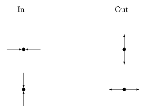
Figure 1: Non-trivial collisions of the HPP lattice-gas: The dynamics takes place on a cartesian lattice in two dimensions. A pair of incoming particles with opposite velocities in the North-South direction become a pair of particles with opposite velocities in the East-West direction, and vice versa.

The simplest two-dimensional example of a lattice-gas model is the HPP model Hardy et al. (1973). Here, the underlying lattice is cartesian, hence there are four lattice vectors per site, corresponding to a particle moving north, east, south, or west. There may be at most one particle per direction per site, leading to at most four particles at each lattice site. The non-trivial collision of the HPP gas is shown in Figure 1.

The distinction between cellular automata and lattice-gases has been the source of some debate Toffoli et al. (2008); Henon (1989). A homogeneous cellular automata utilizes the same neighborhood and the same update rule at every site and every timestep, as in the Game of Life. The lattice-gas evolves in two distinct substeps: propagation and collision (described in detail below). The connection between the models may be made by introducing the concept of a block- or partitioned- cellular automata, which alternates between two update rules and two neighborhoods. The simplest of these automata employ a Margolus neighborhood Margolus (1984). As an example, we shall construct the two rules and two neighborhoods which, when alternately applied to a cellular automata, yield the HPP lattice-gas dynamics described above. The update rules are shown in Figure 2. The update rules act on a block of four cells, which we shall refer to as upper left (UL), upper right (UR), lower left (LL), lower right (LR). The propagation rule is applied identically to all states: the occupation of each cell in the four cell block is exchanged with the occupation of the cell diagonally opposite. The collision step is identical to the propagation step except when UR and LL are the only cells occupied or when LR and UL are the only cells occupied, in which case the occupancies of these pairs of cells are exchanged. Graphically this corresponds to either diagonal of the four cells being occupied. In these cases the state is flipped to the other diagonal occupation, as shown in Figure 2.

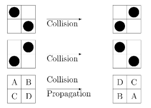
Figure 2: Update rules for the HPP partitioned cellular automata. The top two boxes show the collision rules in which the configurations of the cells which are modified in a non-trivial way. The bottom boxes show the update rule which implements propagation in the automata. The bottom rule is applied to both neighborhoods of the automata. $A,B,C,D$ represent any occupation state of the four cells, and the propagation update is the permutation of these occupations shown.

Clearly, if either of these rules was applied to a constant neighborhood the resulting dynamics would be trivial. Neither rule can change the occupation outside the four cell block and both rules are self inverse, so applying them twice to the same block returns the original configuration. In our partitioned automata we specify a different neighborhood for each rule in order to obtain the HPP dynamics. The Margolus neighborhoods, the cells of the automata and their relationship to the original cartesian lattice on which we defined HPP model are shown in Figure 3. The two neighborhoods are the two ways of partitioning a cartesian grid into square tiles of four cells. The original cartesian lattice on which the HPP lattice gas was defined is the lattice of diagonals with a lattice node at the center of every collision neighborhood. The lattice-gas vertices are shown by open circles in the third Figure in Figure 3.

(a) Collision neighborhood

(b) Propagation neighborhood

(c) Lattice-gas sites and particle directions

Figure 3: Neighborhoods for collision (a) and propagation (b). The boundaries of the four cell blocks on which the rules shown in Figure 2 are applied are shown by the bold lines. Figure (a) shows the boundaries for the collision neighborhood. Figure (b) shows the boundaries for the propagation neighborhood. Figure (c) shows the correspondence between the cells of the partitioned automata and the lattice of the lattice-gas. Bold lines denote the directions along which lattice-gas particles move. Open circles denote sites of the lattice-gas.

In this approach, the original cells of the automata are grouped together into blocks of four to make the sites of the HPP lattice-gas model. The partitioned dynamics is reinterpreted - one step of the dynamics (which acts on one partitioning of the original cells) now acts locally on a single lattice-gas site. This local action is termed the collision or scattering step. The second step of the dynamics (which acts on the other partitioning of the original cells in the Margolus scheme Margolus (1984)) implements propagation of information between the lattice-gas sites. In the case of the HPP model, where the alphabet of the original cells is $\{0,1\}$, this step has the interpretation of particles moving from one lattice-gas site to another. The four sub-cells of a lattice-gas site are then reinterpreted as lattice vectors, and in the propagation step lattice-gas particles move in the direction of their lattice vector to a new site. Hence we have taken a partitioned cellular automata and reverse-engineered a lattice-gas model from it.

The general question of when a classical cellular automata can be reinterpreted in this way was recently taken up in Toffoli et al. (2008). Because we know, from the example of Arrighi et al. (2008), that there are QCA that are not partitioned CA, we shall proceed by first defining classical lattice-gas automata and proving a general condition for when a QCA is a QLGA. In the process we shall extend our definition of a classical lattice-gas to the quantum case.

Consider the lattice to be $\mathbb{Z}^{n}$. Each point $x$ on this lattice is a site of the lattice-gas and has the same neighborhood $\mathcal{N}_{x}$. We may consider each neighborhood $\mathcal{N}_{x}$ to be a translation (by $x$) of the neighborhood $\mathcal{N}$ of the site $x=0$, where $\mathcal{N}$ is a finite subset of $\mathbb{Z}^{n}$. Hence the neighborhood of site $x$ is given by ${x+z|z\in\mathcal{N}}$. The state of a single site may be constructed by assigning a substate to each of a set of lattice vectors - each vector corresponding to a neighborhood element $z\in\mathcal{N}$. The sub-state ${\bf k}_{x}(z)$ of each lattice vector $z$ at lattice site $x$ takes values in an alphabet $\mathcal{C}_{z}$. For the simplest lattice-gases, each lattice vector may have either one or zero particles present and so $\mathcal{C}_{z}=\{0,1\}~{}\forall~{}z$. However, more sophisticated models allow multiple types of particles, and three-dimensional models allow some vectors to carry more than one particle Boghosian et al. (2000), hence in general $\mathcal{C}_{z}$ may contain arbitrarily many symbols and may vary with $z$. The state ${\bf k}_{x}$ of a lattice-gas site $x$ is therefore an element of the Cartesian product of all of the $\mathcal{C}_{z}$:

$${\bf k}_{x}=\prod_{z\in\mathcal{N}}{\bf k}_{x}(z)\in B=\prod_{z\in\mathcal{N}}\mathcal{C}_{z}$$ (1)

The state of the lattice-gas is an element of the set of infinite sequences $\mathcal{S}$ over $B$.

We may now define the two substeps of the lattice-gas dynamics. Firstly, the sub-states propagate to the lattice sites in the neighborhood:

$$\sigma:\mathcal{S} \longrightarrow\mathcal{S}$$

$$\prod_{x\in\mathbb{Z}^{n}}\prod_{z\in\mathcal{N}}{\bf k}_{x}(z) \mapsto\prod_{x\in\mathbb{Z}^{n}}\prod_{z\in\mathcal{N}}{\bf k}_{x+z}(z)$$

Secondly, in the collision step, the state of each lattice-gas site changes locally under a map $\Theta$:

$$\Theta:\prod_{z\in\mathcal{N}}\mathcal{C}_{z}\longrightarrow\prod_{z\in\mathcal{N}}\mathcal{C}_{z}.$$ (2)

With these classical definitions in hand, we now turn to the definition of quantum cellular automata.

I.2 Watrous Quantum Cellular Automata

QCA have been studied, in considerable depth, by several authors Watrous (1995); van Dam (1996); Durr et al. (1996); Dürr and Santha (2002); Arrighi (2006); Schumacher and Werner (2004); Arrighi et al. (2008). The main idea is to develop quantum models that retain the key features of a classical cellular automata: translation invariance and discreteness in time, space and dynamical variables. A classical deterministic cellular automata is defined as follows:

1. A lattice $\mathcal{L}$, whose sites we shall label by $x$.

2. A set of cell values $Q$ with a distinguished quiescent state $q_{0}$.

3. A neighborhood $\mathcal{N}$. This translates to a neighborhood $\mathcal{N}_{x}$ for each cell $x$, consisting of a set of cells as follows: $\mathcal{N}_{x}=\{x+z|z\in\mathcal{N}\}$.

4. A configuration of the automata is a map $a:L\longrightarrow Q$. If $L$ is infinite then only a finite number of cells take values in $Q$ that are not quiescent.

5. A local transition rule $\delta$ which updates the value $s_{x}\in Q$ at $x$ according to the values $s_{i}\in Q$ (where $i\in\mathcal{N}_{x}$) of the cells in the neighborhood $\delta:Q^{|\mathcal{N}|}\mapsto Q$, subject to the condition that

   $$\delta:q_{0}^{|\mathcal{N}|}\mapsto q_{0}.$$ (3)

Early work produced an extension of the classical cellular automata (CA) defined above based on local rules Meyer (1996c); van Dam (1996); Durr et al. (1996); Dürr and Santha (2002); Arrighi (2006). To avoid confusion with the definition of a Quantum Cellular Automata (QCA) that we shall introduce later we follow Schumacher and Werner (2004) and call these Watrous Quantum Cellular Automata (WQCA). A WQCA is defined as follows:

1. A lattice ${L}$, whose sites we shall label by $x$.

2. A set of cell values $Q$ with a distinguished quiescent state $q_{0}$.

3. A neighborhood $\mathcal{N}$. This translates to a neighborhood $\mathcal{N}_{x}$ for each cell $x$, consisting of a set of cells as follows: $\mathcal{N}_{x}=\{x+z|z\in\mathcal{N}\}$.

4. A state of the automaton, $\Psi$, is a superposition of classical configurations.

5. A local evolution rule $f$ which maps an element of $Q^{|\mathcal{N}|}$ to an element of $W=\mathbb{C}[Q]$,

   $$f:Q^{|\mathcal{N}|}\longrightarrow\mathbb{C}[Q]$$

   subject to the constraint that if the neighborhood state is $q_{0}^{|\mathcal{N}|}$ then $f$ assigns amplitude $1$ to the quiescent state and amplitude $0$ to all other states.

From the above data, one can construct a global evolution rule $R$ by jointly evolving the state of each cell $x$ in any basis state by the local rule $f$ and extending by linearity. The global evolution $R$ is required to be:

1. Unitary: $R^{\dagger}R=\mathbb{I}$.

2. Translation invariant: Let $\tau_{z}$, for some $z\in\mathbb{Z}$, be the translation operator defined by its action on a classical configuration $c=\prod_{j\in\mathbb{Z}}c_{j}$ for $c_{j}\in Q~{}\forall~{}j$:

   $$\tau_{z}:\prod_{j\in\mathbb{Z}}c_{j}\mapsto\prod_{j\in\mathbb{Z}}c_{j+z}$$

   $\tau_{z}$ is extended by linearity. We denote the group of translations: $\mathcal{T}=\{\tau_{z}\}_{z\in\mathbb{Z}}$. A linear operator $R$ is translation-invariant if $\tau_{z}R\tau^{-1}_{z}=R$ for all $z\in\mathbb{Z}$.

By definition, the above model of WQCA is translation-invariant provided the rule $f$ is the same for all cells. Unitarity for this model has been extensively investigated Meyer (1996c); van Dam (1996); Durr et al. (1996); Dürr and Santha (2002). This model of QCA was found Arrighi et al. (2008), in some instances of the finite, unbounded QCA, to allow super-luminal signaling. Super-luminal signaling refers to the faster than light signaling which occurs when the state of a cell (restricted or reduced state, defined in the next section) can be affected by that of another cell which is an unbounded distance away from it. This is observed when certain classical CAs with finite neighborhood schemes are quantized (the local rule for classical CA is taken as that for the QCA).

I.3 Axiomatic QCA

An axiomatic approach has been developed to overcome the problem of super-luminal signaling, a non-local phenomenon, seen in the WQCA models Schumacher and Werner (2004); Arrighi et al. (2008, 2011); Schumacher and Westmoreland (2005). The requirement of causality is imposed in the definition of a QCA, with roots in the ideas of Beckman et al. (2001); Schumacher and Westmoreland (2005), to preclude this non-locality Cheung and Perez-Delgado (2007); Schumacher and Werner (2004); Arrighi et al. (2008, 2011).

The axiomatic model was introduced by Schumacher and Werner in Schumacher and Werner (2004) and further developed by Arrighi, Nesme, and Werner in Arrighi et al. (2008). In this approach a QCA is defined to be a unitary, translation-invariant, $*$-homomorphism of a $C^{*}$ -algebra which satisfies a quasi-local condition by which the global homomorphism R is uniquely determined by a local homomorphism of tensor factor (one-site) algebras to the neighborhood. The program developed in Schumacher and Werner (2004) investigates when the structure of such QCA s can be given by $*$-isomorphisms obeying a quasi-local condition as follows. Once the cells are grouped into super-cells, such super-cells partition the lattice. Then there exists a shifted partition with super-cells that overlap with the original cells in a Margolus partitioning scheme Margolus (1984). The global evolution is given by a set of unitary operators U, V, each of which acts on a cell of the respective partition, applied in succession. If this structure holds, then imposing the requirement of causality on quantum cellular automata requires them to be quantum lattice-gas automata.

One of the conclusions of Schumacher and Werner in Schumacher and Werner (2004), that all QCA are QLGA, was revised by Arrighi, Nesme, and Werner in Arrighi et al. (2008). Arrighi, Nesme, and Werner Arrighi et al. (2008) give an example of a QCA in Arrighi et al. (2008) that is not a QLGA, thus showing that there is a separation between two non-empty subclasses of QCA. Precisely characterizing this separation by determining which QCA are QLGA is the subject of the present paper. The axiomatic one-dimensional development of Arrighi, Nesme, and Werner Arrighi et al. (2008) is more restricted and defined on a Hilbert space of unbounded, finite configurations (finitely many active cells in a quiescent background). This set of sequences, called the set of finite configurations, is embedded into some abstract Hilbert space in which the elements of this set comprise an orthonormal basis. This is a countable-dimensional Hilbert space the Hilbert space of finite configurations. In this context, they define a QCA as a unitary, translation-invariant and causal operator on the Hilbert space of finite configurations.

In the present work we further develop the axiomatic approach and place it on a new mathematical foundation. We incorporate in the development of axiomatic QCAs the topology of the Hilbert space. This is an essential part of any study of the algebra of operators, particularly infinite dimensional algebras. This is intimately connected, in this case, with the idea of local algebras and the part they play in the determination of the global evolution. This topology provides the foundation for connecting the local algebras to the algebra of bounded linear operators of the Hilbert space. With this topology, we can investigate the space of bounded linear operators as a von Neumann Algebra (as well as a $C^{*}$ algebra), making the local subalgebras a useful tool.

We develop a model on the same space of finite but unbounded configurations as Arrighi, Nesme, and Werner Arrighi et al. (2008). To make a Hilbert space from it, we give an inner product structure to the set of finite configurations that is a natural extension of the inner product of the Hilbert space of each cell. We define the Hilbert space of finite configurations as the $\ell^{2}$ completion of the linear span of the set of finite configurations. This defines the separable topology of the Hilbert space and the induced inner product is used to define the norm, weak, and strong topologies of the bounded linear operators on the space. At the outset, we show how the subalgebra of local finite dimensional operators is connected to the algebra of bounded linear operators on the whole space (Theorem III.7, the Density Theorem). This provides the background for the development of some of the key ideas, and underpins the proof of the Structural Reversibility Theorem (Arrighi, Nesme, and Werner Arrighi et al. (2008)).

The main result of this paper is that QLGA can be characterized by a local condition on QCA. This condition pertains to the set of image algebras under the global evolution of the neighboring cells. The condition for a QCA to be a QLGA is that the local pieces of these image algebras generate the full cell algebra. It is clear from our development that a central result, Theorem III.10, about the tensor product decomposition of Hilbert space of a single cell is not true in general. In particular, to have that decomposition, the aforementioned subalgebra condition is needed. This condition is not satisfied for all QCA, as shown by the example in Arrighi et al. (2008). This means that there is a class of QCAs that are not QLGAs and that require further exploration.

The current paper is structured as follows. In Section II we introduce the Hilbert space of interest for our automata. In Section III we introduce the axiomatic definition of QCA and prove several properties of operators that are translation invariant or causal, or both. We extend our definitions of the propagation and collision operators to the quantum case and formally define a QLGA before proving our main theorem. In Section IV we give a number of examples of QCA, for the case when our condition is satisfied and when it is not. We close the paper with some conclusions and discussion. In the interests of making the present paper self contained we collect a number of background and corollary results in the appendices.

II The Hilbert space of finite configurations

We begin with a finite set of symbols $Q$ containing a special quiescent symbol $q_{0}$, and an infinite lattice $\mathcal{L}=\mathbb{Z}^{n}$ in $n$ dimensions. Let us denote by $W$ the Hilbert space of formal linear combinations of symbols in $Q$, i.e. $W=\mathbb{C}[Q]$ (in this paper all of the vector spaces will be over $\mathbb{C}$). This Hilbert space $W$ is the Hilbert space of quantum states of a single cell (for the rest of the paper, we will use the terms cell and site to mean an element of the lattice $\mathcal{L}$). Let the dimension of $W$ (cardinality of $Q$) be $\text{dim}W=d_{W}$. The set of basis elements of $W$ corresponding to the symbols in $Q$ is denoted $B_{Q}$:

$$B_{Q}=\{\left|q\right\rangle:q\in Q\}$$ (4)

$W$ has an inner product:

$$\langle\alpha|\vartheta\rangle=\sum_{q\in Q}\overline{\alpha_{q}}\vartheta_{q}$$ (5)

where $\alpha=\sum_{q\in Q}\alpha_{q}|q\rangle$, $\vartheta=\sum_{q\in Q}\vartheta_{q}|q\rangle$.

Informally, the Hilbert space of the automata is the infinite tensor product of copies of $W$. The idea of infinite tensor products was first studied by von Neumann in his landmark paper “On Infinite Direct Products” von Neumann (1939). Later, Guichardet Guichardet (1972) introduced a more modern way of describing an infinite tensor product of Hilbert spaces enumerated by a countable set. This is sometimes referred to as the incomplete tensor product construction. From countably many copies of the same Hilbert space $W$ the incomplete tensor product is obtained as the inductive limit of an ascending chain of finite tensor products of $W$. This space has a natural basis that we call the set of finite configurations. The Hilbert space of finite configurations is the incomplete tensor product construction of Guichardet with the set of finite configurations as its basis Guichardet (1972).

Definition II.1.

The set of finite configurations, denoted by $\mathcal{C}$, is the set of simple tensor products with only finitely many active elements,

$$\mathcal{C}:=\{\bigotimes_{x\in\mathbb{Z}^{n}}|c_{x}\rangle:|c_{x}\rangle\in B_{Q},\text{ all but finite }|{c}_{x}\rangle=|q_{0}\rangle\}$$

Thus, $\mathcal{C}$ is a countably infinite set. Let $|c\rangle=\bigotimes_{x\in\mathbb{Z}^{n}}|c_{x}\rangle,|c^{\prime}\rangle=\bigotimes_{x\in\mathbb{Z}^{n}}|{c_{x}}^{\prime}\rangle\in\mathcal{C}$. Define the inner product of the elements $|c\rangle$, $|c^{\prime}\rangle$:

$$\langle c|c^{\prime}\rangle=\prod_{x\in\mathbb{Z}^{n}}\langle c_{x}|{c_{x}}^{\prime}\rangle$$

and extend it by linearity to get an inner product on span($\mathcal{C}$) (the set of finite linear combinations of elements of $\mathcal{C}$).

Definition II.2.

The Hilbert space of finite configurations, denoted by $\mathcal{H}_{\mathcal{C}}$, is the ${\ell}^{2}$ completion of $\text{span}(\mathcal{C})$ under the norm induced by the above inner product. $\mathcal{C}$ constitutes an orthonormal basis of $\mathcal{H}_{\mathcal{C}}$.

By definition, $\mathcal{H}_{\mathcal{C}}$ is a separable Hilbert space since it has a countable orthonormal basis $\mathcal{C}$ (this follows from a standard theorem on Hilbert spaces in texts on analysis, for example, Folland Folland (1999), Proposition 5.29, pg. 176).

Definition II.3.

The neighborhood $\mathcal{N}\subset\mathbb{Z}^{n}$ is some finite set. The neighborhood of a cell $x\in\mathbb{Z}^{n}$, denoted by $\mathcal{N}_{x}$, is a translation of $\mathcal{N}$ to $x$.

$$\mathcal{N}_{x}=\{k+x:k\in\mathcal{N}\}$$

The state of the QCA, $\rho$, is described by a density operator.

Definition II.4.

A density operator, $\rho$, is a positive trace class operator on $\mathcal{H}_{\mathcal{C}}$, with tr($\rho$) =  1.

III Axiomatic Definition of QCA

In this section we introduce the axiomatic definition of QCA in which the requirement of causality is built in from the start. We show that a QCA on the Hilbert space of finite configurations must possess a quiescent state as an eigenstate of its global evolution. We define local operators, and connect the algebraic structure of these operators to the topological structure of operators on the Hilbert space of finite configurations. We then consider the action of the global evolution operator on the local operators and define the requirement of causality in terms of the evolution of local operators. This definition of causality in the Heisenberg picture was termed dual causality or structural reversibility by Schumacher and Werner (2004) and  Arrighi et al. (2008). Structural reversibility is useful because it means that the analysis of the causal global evolution can proceed by analysis of finite dimensional algebras of local operators.

We continue from the definitions of Section II. We need a few more definitions to properly state the requirements for an axiomatic model of QCA. For a finite subset $D\in\mathbb{Z}^{n}$, we introduce the idea of a co-$D$ space, which will be of use for a number of results.

Definition III.1.

Let $D\in\mathbb{Z}^{n}$ be a finite subset. Define the set of co-$D$ configurations to be $\mathcal{C}_{\overline{D}}:=\{\bigotimes_{i\in\mathbb{Z}^{n}\setminus D}|{c}_{i}\rangle:{c}_{i}\in{Q},\text{ all but finite }|{c}_{i}\rangle=|{q}_{0}\rangle\}$. Let the inner product on $\mathcal{C}_{\overline{D}}$ be induced by the inner product on $W$ (5), as in the case of ${\mathcal{C}}$. Then the co-$D$ space, denoted $\mathcal{H}_{{\mathcal{C}}_{\overline{D}}}$, is defined as the completion of $\text{span}({\mathcal{C}}_{\overline{D}})$ under the induced $\ell^{2}$ norm.

Any operator $E\in B(\mathcal{H}_{{\mathcal{C}}})$ can be expressed as a finite sum:

$$E=\sum_{l}e_{l}\otimes E_{l}$$ (6)

where $\{e_{l}\}\subset\text{End}(\bigotimes_{k\in D}W)$ is a linearly independent set, and $\{E_{l}\}\subset B(\mathcal{H}_{{\mathcal{C}}_{\overline{D}}})$.

We can define partial trace on trace class operators in general, and in particular on density operators. We let $\{|w_{x}\rangle\}$ be some orthonormal basis of the co-$D$ space $\mathcal{H}_{{\mathcal{C}}_{\overline{D}}}$. Then a density operator $\rho$ can be expressed as:

$$\rho=\sum_{x,y}\rho_{x,y}\otimes|w_{x}\rangle\langle w_{y}|$$

where $\rho_{x,y}\in\rm{End}(\bigotimes_{j\in D}W_{j})$. The partial trace of $\rho$ over the tensor factors not in $D$, denoted $\text{tr}_{\{x\notin D\}}$, is the sum:

$$\text{tr}_{\{x\notin D\}}(\rho):=\sum_{y}\rho_{y,y}.$$

The sum converges, and the definition is independent of the choice of basis $\{|w_{y}\rangle\}$ since $\rho$ is trace class.

We define the restricted or reduced density operator.

Definition III.2.

Let $D\in\mathbb{Z}^{n}$ be a finite subset. Let $\rho$ be a state (density operator) on ${\mathcal{H}}_{\mathcal{C}}$. The restriction of $\rho$ to $D$, denoted $\rho|_{D}$, is defined to be the partial trace of $\rho$ over the tensor factors not in $D$:

$$\rho|_{D}:=\text{tr}_{\{x\notin D\}}(\rho).$$

Now we have the terminology to state the requirements for an axiomatic QCA.

Definition III.3.

The global evolution $R$ of a QCA on the Hilbert space of finite configurations ${\mathcal{H}}_{\mathcal{C}}$, with neighborhood $\mathcal{N}$, is required to be:

1. Unitary: $R^{\dagger}R=\mathbb{I}$.

2. Translation invariant: Let $\tau_{z}$, for some $z\in\mathbb{Z}^{n}$, be the translation operator defined by its action on an element $|c\rangle=\bigotimes_{j\in\mathbb{Z}^{n}}|c_{j}\rangle\in\mathcal{C}$:

   $$\tau_{z}:\bigotimes_{j\in\mathbb{Z}^{n}}|c_{j}\rangle\mapsto\bigotimes_{j\in\mathbb{Z}^{n}}|c_{j+z}\rangle$$

   The map $\tau_{z}$ is extended by linearity to span($\mathcal{C}$), on which it is inner product preserving. Then $\tau_{z}$ can be unitarily extended to ${\mathcal{H}}_{\mathcal{C}}$ (that such an extension exists, and is a unitary operator on ${\mathcal{H}}_{\mathcal{C}}$, follows from the Bounded Linear Transformation (B.L.T.) Theorem, standard in the theory of operators on Banach spaces. The reader can find it in Reed and Simon Reed and Simon (1980) as Theorem 1.7, pg. 9). We denote the group of translations: $\mathcal{T}=\{\tau_{z}\}_{z\in\mathbb{Z}^{n}}$. A linear operator $M$ on ${\mathcal{H}}_{\mathcal{C}}$ is translation-invariant if $\tau_{z}M\tau^{-1}_{z}=M$ for all $z\in\mathbb{Z}^{n}$.

3. Causal relative to the neighborhood $\mathcal{N}$: A linear operator $M$ on ${\mathcal{H}}_{\mathcal{C}}$ is said to be causal relative to a neighborhood $\mathcal{N}$ if for every pair $\rho,\rho^{\prime}$, of density operators, and $x\in\mathbb{Z}^{n}$, that satisfy:

   $$\rho|_{\mathcal{N}_{x}}=\rho^{\prime}|_{\mathcal{N}_{x}}\text{,}$$

   the operators $M\rho M^{\dagger},M\rho^{\prime}M^{\dagger}$ satisfy:

   $$M\rho M^{\dagger}|_{x}=M\rho^{\prime}M^{\dagger}|_{x}$$

Let us see what the constraints of Definition III.3 tell us about an operator. First we consider translation-invariance. We begin by identifying the invariants (the fixed points), in ${\mathcal{H}}_{\mathcal{C}}$, of the group of translations $\mathcal{T}=\{\tau_{z}\}_{z\in\mathbb{Z}^{n}}$.

Lemma III.4.

The space of $\mathcal{T}$-invariants in ${\mathcal{H}}_{\mathcal{C}}$ is one-dimensional. It is: $\mathbb{C}^{\times}\bigotimes_{x\in\mathbb{Z}^{n}}|q_{0}\rangle$, where $\mathbb{C}^{\times}=\mathbb{C}\setminus\{0\}$.

Proof.

Consider the action of $\mathcal{T}$ on ${\mathcal{H}}_{\mathcal{C}}$. Let us write $\phi\in{\mathcal{H}}_{\mathcal{C}}$ in a basis $\{|C_{i}\rangle:i\in\mathbb{Z}\}$ of ${\mathcal{H}}_{\mathcal{C}}$ :

$$\phi=\sum_{i\in\mathbb{Z}}\phi_{i}|C_{i}\rangle$$

where $|C_{i}\rangle\in\mathcal{C}$. Let $|C_{0}\rangle=\bigotimes_{x\in\mathbb{Z}^{n}}|q_{0}\rangle$. If $\tau_{z}\in\mathcal{T}$, then:

$$\tau_{z}(\phi)=\tau_{z}(\sum_{i}\phi_{i}|C_{i}\rangle)=\sum_{i\in\mathbb{Z}}\phi_{i}\tau_{z}(|C_{i}\rangle)$$

Since $\tau_{z}$ permutes elements of $\mathcal{C}$, we can associate a permutation $s_{z}$ of the indices $i\in\mathbb{Z}$ with the action of $\tau_{z}$, i.e., $\tau_{z}(|C_{i}\rangle)=|C_{s_{z}(i)}\rangle$.

If $\phi$ is an invariant of $\mathcal{T}$, then: $\tau_{z}(\phi)=\phi$ for all $z\in\mathbb{Z}^{n}$, i.e.,

$$\sum_{i\in\mathbb{Z}}\phi_{i}|C_{i}\rangle=\sum_{i\in\mathbb{Z}}\phi_{i}\tau_{z}(|C_{i}\rangle)=\sum_{i\in\mathbb{Z}}\phi_{{s_{z}}^{-1}(i)}|C_{i}\rangle$$

This implies $\phi_{i}=\phi_{{s_{z}}^{-1}(i)}$ for $z\in\mathbb{Z}^{n}$, i.e., $\phi_{i}$ are constant on the orbits of $\mathcal{C}$ under the action of $\mathcal{T}$. But $\mathcal{T}$ fixes $|C_{0}\rangle=\bigotimes_{x\in\mathbb{Z}^{n}}|q_{0}\rangle$, and all other orbits in $\mathcal{C}$ are countably infinite in cardinality. Since $\phi$ has a finite $\ell^{2}$ norm, this implies that $\phi_{i}=0$ for all $i\neq 0$, i.e., the space of $\mathcal{T}$-invariants is one-dimensional: $\mathbb{C}\bigotimes_{x\in\mathbb{Z}^{n}}|q_{0}\rangle$. ∎

Now that we know that the only vectors fixed by the group of translations are scalar multiples of the quiescent state: $\bigotimes_{x\in\mathbb{Z}^{n}}|q_{0}\rangle$, we go on to determine the action of invertible translation-invariant operators on the quiescent state.

Lemma III.5.

An invertible and translation-invariant operator $M$ on ${\mathcal{H}}_{\mathcal{C}}$ has $\bigotimes_{x\in\mathbb{Z}^{n}}|q_{0}\rangle$ as an eigenvector:

$$M\big{(}\bigotimes_{x\in\mathbb{Z}^{n}}|q_{0}\rangle\big{)}=\lambda_{0}\bigotimes_{x\in\mathbb{Z}^{n}}|q_{0}\rangle$$

for some $\lambda_{0}\in\mathbb{C}^{\times}$. In particular, if $M$ is unitary and translation-invariant, then $\lambda_{0}=e^{i\Theta_{0}}$ for some $\Theta_{0}\in\mathbb{R}$.

Proof.

$M$ is invertible, so $M\big{(}\bigotimes_{x\in\mathbb{Z}^{n}}|q_{0}\rangle\big{)}\neq 0$. And $M$ is translation invariant, hence:

$$\tau_{z}M\tau_{z}^{-1}\big{(}\bigotimes_{x\in\mathbb{Z}^{n}}|q_{0}\rangle\big{)}=M\big{(}\bigotimes_{x\in\mathbb{Z}^{n}}|q_{0}\rangle\big{)}\quad\forall z\in\mathbb{Z}^{n}$$

But $\tau_{z}^{-1}(\bigotimes_{x\in\mathbb{Z}^{n}}|q_{0}\rangle)=\bigotimes_{x\in\mathbb{Z}^{n}}|q_{0}\rangle$ for all $z\in\mathbb{Z}^{n}$. This implies:

$$\tau_{z}\bigg{(}M\big{(}\bigotimes_{x\in\mathbb{Z}^{n}}|q_{0}\rangle\big{)}\bigg{)}=M\big{(}\bigotimes_{x\in\mathbb{Z}^{n}}|q_{0}\rangle\big{)}\quad\forall z\in\mathbb{Z}^{n}$$

that is, $M\big{(}\bigotimes_{x\in\mathbb{Z}^{n}}|q_{0}\rangle\big{)}$ is an invariant of $\tau_{z}$ for all $z\in\mathbb{Z}^{n}$. Lemma III.4 now implies that:

$$M\big{(}\bigotimes_{x\in\mathbb{Z}^{n}}|q_{0}\rangle\big{)}=\lambda_{0}\bigotimes_{x\in\mathbb{Z}^{n}}|q_{0}\rangle$$

for some $\lambda_{0}\in\mathbb{C}^{\times}$.

As a special case, if $M$ is unitary then all its eigenvalues are roots of unity and so $\lambda_{0}=e^{i\Theta_{0}}$ for some $\Theta_{0}\in\mathbb{R}$. ∎

Finally, we consider the implication of causality on a unitary operator. First we need the related notion of a local operator. For any finite-dimensional vector spaces $V$ and $W$, we will assume the standard isomorphisms: ${\rm End}(V)\cong V\otimes V^{*}$ and ${\rm End}(V\otimes W)\cong{\rm End}(V)\otimes{\rm End}(W)$, and make use of them as needed, without explicit mention. Consider the embedding of $\bigotimes_{j\in D}\rm{End}(W)$ into a subalgebra of $B({\mathcal{H}}_{\mathcal{C}})$ (the algebra of bounded linear operators on $\mathcal{H}_{\mathcal{C}}$, where the norm is the usual operator norm):

$$\iota_{D}:\bigotimes_{j\in D}\rm{End}(W) \hookrightarrow B({\mathcal{H}}_{\mathcal{C}})$$ (7)

$$a \mapsto a\otimes\mathbb{I}_{\overline{\mathcal{D}}}$$

where $a$ is an element of $\bigotimes_{j\in D}\rm{End}(W)$, and $\mathbb{I}_{\overline{\mathcal{D}}}$ is the identity operator on the co-$D$ space, $\mathcal{H}_{{\mathcal{C}}_{\overline{D}}}$, with the operator decomposition as in (6). Through the embedding $\iota_{D}$ (7) the algebra $\bigotimes_{j\in D}\rm{End}(W)$ is isomorphic to the corresponding finite dimensional subalgebra of $B({\mathcal{H}}_{\mathcal{C}})$.

Definition III.6.

An operator $M$ on ${\mathcal{H}}_{\mathcal{C}}$ is local upon a finite subset $D\in\mathbb{Z}^{n}$ if it is in the image of the map $\iota_{D}$ (7).

To understand the significance of these local subalgebras, we connect the algebraic structure of the subalgebra they generate to the topological structure of $B({\mathcal{H}}_{\mathcal{C}})$. Let us denote the subalgebra embeddings (7) by $\mathcal{A}_{D}=\iota_{D}(\bigotimes_{j\in D}\rm{End}(W))$. Let $\{D_{k}\subset\mathbb{Z}^{n}:|D_{k}|<\infty\}_{k\in\mathbb{N}}$ be a strictly ascending chain:

$$D_{0}\subsetneq D_{1}\subsetneq\ldots$$

such that: $\mathbb{Z}^{n}=\cup_{k\in\mathbb{N}}D_{k}$. We have an ascending chain of subalgebras formed by embeddings $\{\mathcal{A}_{D_{k}}\}_{k\in\mathbb{N}}$, and we denote the union of these subalgebras by $\mathcal{Z}$:

$$\mathcal{Z}=\cup_{k}\mathcal{A}_{D_{k}}$$ (8)

For the proof of the next theorem, we need the following definition. Define, for any subset $\mathcal{S}\subset B({\mathcal{H}}_{\mathcal{C}})$, the commutant of $\mathcal{S}$:

$$\text{Comm}(\mathcal{S})=\{y\in B({\mathcal{H}}_{\mathcal{C}}):ys=sy\>\>\forall s\in\mathcal{S}\}$$

Theorem III.7 (Density Theorem).

$\mathcal{Z}$ is dense in $B({\mathcal{H}}_{\mathcal{C}})$ in the weak and strong operator topologies.

Proof.

$\mathcal{Z}$ acts irreducibly on $\mathcal{H}_{\mathcal{C}}$. Indeed, $\mathcal{Z}$ acts transitively on a dense subspace, $\text{span}(\mathcal{C})$, of $\mathcal{H}_{\mathcal{C}}$. This implies, by Schur’s Lemma (Lemma A.1), Comm$(\mathcal{Z})=\mathbb{C}\mathbb{I}$ , where $\mathbb{I}$ is the identity operator on $\mathcal{H}_{\mathcal{C}}$. Then Comm(Comm($\mathcal{Z}))=B({\mathcal{H}}_{\mathcal{C}})$. By von Neumann Density theorem (Theorem A.8), Comm(Comm($\mathcal{Z}$)) is the weak and strong closure of $\mathcal{Z}$. ∎

The embedding $\iota_{D}$ (7) allows us to consider the individual elements of $\mathcal{A}_{x}$ (the special case when $D=\{x\}$, i.e., a single cell) as acting only on the tensor factors of interest. Then we are justified, for notational reasons, in replacing the finite dimensional algebras $\mathcal{A}_{D}$ with a finite tensor product of cell algebras of the form $\mathcal{A}_{x}$.

For a unitary operator $M$ on $B(\mathcal{H}_{\mathcal{C}})$, denote by $C_{M}$, the conjugation by $M$ map on $B(\mathcal{H}_{\mathcal{C}})$:

$$C_{M}:B(\mathcal{H}_{\mathcal{C}}) \longrightarrow B(\mathcal{H}_{\mathcal{C}})$$

$$Z \mapsto M^{\dagger}ZM$$

As $M$ is assumed to be unitary, this map is a unitary isomorphism (under the usual operator norm) of $B({\mathcal{H}}_{\mathcal{C}})$.

For any set $Y\subset B(\mathcal{H}_{\mathcal{C}})$ the image of $Y$ under conjugation by $M$ is $C_{M}(Y)$. By abuse of notation, we say, $C_{M}(Y)=M^{\dagger}YM$. The images of the cell algebras under conjugation by $M$, $\mathcal{M}_{z}=M^{\dagger}\mathcal{A}_{z}M$, $z\in\mathbb{Z}^{n}$ are finite dimensional, and for $z,z^{\prime}\in\mathbb{Z}^{n}$, $z\neq z^{\prime}$, $\mathcal{M}_{z}$, $\mathcal{M}_{z^{\prime}}$ pairwise commute as $\mathcal{A}_{z}$, $\mathcal{A}_{z^{\prime}}$ pairwise commute.

Having defined the local operators we now consider the supports of some such operators of particular interest. Let the reflected neighborhood of $\mathcal{N}$, denoted $\mathcal{V}$, be:

$$\mathcal{V}=-\mathcal{N}=\{-k:k\in\mathcal{N}\}$$

Then this reflected neighborhood $\mathcal{V}$ can also be translated. We denote the translation by $\mathcal{V}_{x}$.

$$\mathcal{V}_{x}=\{x-k:k\in\mathcal{N}\}$$

The size of this set, by definition, is $|\mathcal{V}_{x}|=|\mathcal{N}|$.

It is straightforward to see, by symmetry, that $\mathcal{V}_{x}\subset\mathbb{Z}^{n}$ is the subset of the lattice consisting of those elements whose neighborhood contains $x$:

$$\mathcal{V}_{x}=\{l:x\in\mathcal{N}_{l}\}$$

Causality can be expressed in the Heisenberg picture in which one considers the evolution of operators. This form of causality is captured by the Structural Reversibility theorem due to Arrighi, Nesme, and Werner Arrighi et al. (2008). In the interests of making the present paper self contained we have included the proof of this Theorem in the Appendix (Theorem C.1).

Theorem III.8 (Structural Reversibility).

Let $M:\mathcal{H}_{\mathcal{C}}\longrightarrow\mathcal{H}_{\mathcal{C}}$ be a unitary operator and $\mathcal{N}$ a neighborhood. Let $\mathcal{V}=\{-k|k\in\mathcal{N}\}$. Then the following are equivalent:

1. $M$ is causal relative to the neighborhood $\mathcal{N}$.

2. For every operator $A_{x}$ local upon cell $x$, $M^{\dagger}A_{x}M$ is local upon $\mathcal{N}_{x}$.

3. $M^{\dagger}$ is causal relative to the neighborhood $\mathcal{V}$.

4. For every operator $A_{x}$ local upon cell $x$, $MA_{x}M^{\dagger}$ is local upon ${\mathcal{V}}_{x}$.

The requirement of causal evolution will be useful in the local analysis of the global evolution $R$. This is because, by Theorem III.7 the subalgebra generated by the local algebra is dense in $B({\mathcal{H}}_{\mathcal{C}})$. The unitary, causal evolution of the QCA can therefore be considered in terms of finite dimensional local subalgebras of $B({\mathcal{H}}_{\mathcal{C}})$.

For a site $x$ the set of sites whose neighborhood contains $x$ is $\mathcal{V}_{x}$. We first show that the algebra $\mathcal{A}_{x}$ is a subset of the algebra formed from the span of the images of the local algebras $\mathcal{A}_{k}$ for $k\in\mathcal{V}_{x}$. This result is true for all QCAs.

Theorem III.9.

Let $M$ be a unitary and causal map on $\mathcal{H}_{\mathcal{C}}$ relative to some neighborhood $\mathcal{N}$. Then for every $x\in\mathbb{Z}^{n}$,

$$\mathcal{A}_{x}\subset\rm{span}(\prod_{k\in\mathcal{N}}\mathcal{M}_{x-k})$$

In particular $\mathcal{Z}=M^{\dagger}\mathcal{Z}M$.

Proof.

By Structural Reversibility, Theorem III.8 (iii), for every $x\in\mathbb{Z}^{n}$,

$$M\mathcal{A}_{x}M^{\dagger}\subset\bigotimes_{k\in\mathcal{N}}\mathcal{A}_{x-k}$$

This implies:

$$\mathcal{A}_{x}=M^{\dagger}M\mathcal{A}_{x}M^{\dagger}M\subset M^{\dagger}(\bigotimes_{k\in\mathcal{N}}\mathcal{A}_{x-k})M=\rm{span}(\prod_{k\in\mathcal{N}}M^{\dagger}\mathcal{A}_{x-k}M)=\rm{span}(\prod_{k\in\mathcal{N}}\mathcal{M}_{x-k})$$

The last statement follows by the first statement and Theorem III.8 (ii), i.e.,

$$\mathcal{M}_{z}\subset\bigotimes_{k\in\mathcal{N}}\mathcal{A}_{z+k}\text{ for all }z\in\mathbb{Z}^{n}$$

∎

Consider conjugation by $R$ on $B(\mathcal{H}_{\mathcal{C}})$, where $R$ is the global evolution of a QCA. We denote this map $C_{R}$:

$$C_{R}:B(\mathcal{H}_{\mathcal{C}}) \longrightarrow B(\mathcal{H}_{\mathcal{C}})$$ (9)

$$Z \mapsto R^{\dagger}ZR$$

Denote $\mathcal{R}_{z}=R^{\dagger}\mathcal{A}_{z}R$, the image of cell algebras $\mathcal{A}_{z}$ under conjugation by $R$ (9). This is the algebra of operators which are the images of operators localized on a single cell, after a single timestep of evolution by $R$. We are interested in the intersection of these time evolved algebras with the algebras localized on a single cell. Let us denote by $\mathcal{D}_{z,x}$ the following subalgebra of $\mathcal{R}_{z}$, $z\in\mathbb{Z}^{n}$:

$$\mathcal{D}_{z,x}=\mathcal{R}_{z}\cap\mathcal{A}_{x}$$ (10)

When $z\in\mathcal{V}_{x}$ then $\mathcal{D}_{z,x}$ are the elements of $\mathcal{R}_{z}$ which are contained in $\mathcal{A}_{x}$, where

$$\mathcal{R}_{z}=R^{\dagger}\mathcal{A}_{z}R\subset\bigotimes_{k\in\mathcal{N}_{z}}\rm{End}(W)$$

and:

$$\mathcal{A}_{z}=\underbrace{\rm{End}(W)}_{k=z}\otimes\bigotimes_{k\in\mathcal{N}_{z}\setminus\{z\}}\mathbb{I}_{k}.$$

The subalgebras $\mathcal{D}_{z,x}$ for $z\in\mathcal{V}_{x}$ may be understood intuitively as the subalgebras localized on $x$ that the cell $x$ receives from cells in $\mathcal{V}_{x}$. It turns out that the algebra generated by $\mathcal{D}_{z,x}$ for $z\in\mathcal{V}_{x}$ is the key ingredient in understanding the structure of a subset of QCA. In particular we are interested in the case when the algebra generated by $\mathcal{D}_{z,x}$ for $z\in\mathcal{V}_{x}$ is equal to the full cell algebra $\mathcal{A}_{x}$. We state a preliminary theorem about the structure of $W=\mathbb{C}[Q]$ and the subalgebras $\mathcal{D}_{z,x}$ when this is the case. This is the theorem that allows a local classification of a QCA as a QLGA. Let $\mathcal{D}_{{x-y},x}$ be as defined in (10), where $x\in\mathbb{Z}^{n}$, and $y\in\mathcal{N}$.

Theorem III.10.

Suppose that $R$ is the global evolution of a QCA with neighborhood $\mathcal{N}$. Then $\mathcal{A}_{x}=\rm{span}(\prod_{y\in\mathcal{N}}\mathcal{D}_{{x-y},x})$ if and only if there exists an isomorphism of vector spaces:

$$S:W\longrightarrow\bigotimes_{z\in\mathcal{N}}V_{z}$$

for some vector spaces $\{V_{z}\}_{z\in\mathcal{N}}$. Under the isomorphism $S$, for each $y\in\mathcal{N}$:

$$\mathcal{D}_{{x-y},x}\cong\rm{End}(V_{y})\otimes\bigotimes_{z\in\mathcal{N},z\neq y}\mathbb{I}_{V_{z}}$$

Before proving the theorem, let us state a corollary describing the structure of the algebras $\mathcal{R}_{x}$ under the conditions of the theorem. These algebras $\mathcal{R}_{x}$ are the images of algebras $\mathcal{A}_{x}$ localized on a single cell, after one timestep of the global evolution $R$.

Corollary III.11.

Suppose that $R$ is the global evolution of a QCA with neighborhood $\mathcal{N}$, and satisfies $\mathcal{A}_{x}=\rm{span}(\prod_{y\in\mathcal{N}}\mathcal{D}_{{x-y},x})$. Then:

1. $\mathcal{A}_{x}=\rm{End}(W)\cong\bigotimes_{z\in\mathcal{N}}\rm{End}(V_{z})$, for all $x\in\mathbb{Z}^{n}$.

2. The dimension of $W$, $d_{W}$, is a product of the dimensions of $V_{z}$, $d_{V_{z}}$, i.e., $d_{W}=\prod_{z\in\mathcal{N}}d_{V_{z}}$.

3. $\mathcal{R}_{x}=\rm{span}(\prod_{k\in\mathcal{N}}\mathcal{D}_{x,{x+k}})\cong\bigotimes_{k\in\mathcal{N}}\rm{End}(V_{k})$.

Proof.

(i) and (ii) are obvious from the isomorphism $S$ in Theorem III.10. For the proof of (iii), we note that by definition of $\mathcal{D}_{x,{x+k}}$ (10), $\mathcal{R}_{x}\supset\rm{span}(\prod_{k\in\mathcal{N}}\mathcal{D}_{x,{x+k}})$. But from Theorem III.10, $\rm{span}(\prod_{k\in\mathcal{N}}\mathcal{D}_{x,{x+k}})\cong\bigotimes_{k\in\mathcal{N}}\rm{End}(V_{k})\cong\rm{End}(W)$. We already know that $\mathcal{R}_{x}=R^{\dagger}\mathcal{A}_{x}R\cong\rm{End}(W)$. Hence the conclusion. ∎

This corollary shows that if the conditions of Theorem III.10 are met then the algebra $\mathcal{A}_{x}$ is isomorphic to an algebra generated by a set of commuting algebras each of which is the endomorphisms (full matrix algebra) of a single tensor factor of the space $W$.

The following lemma shows that if there is a set of pairwise commuting self-adjoint algebras that generate $\rm{End}(W)$, then there is a tensor product decomposition of the space $W$ such that each of the commuting self-adjoint algebras is the set of endomorphisms (full matrix algebra) of one of the tensor factors. This will be useful in the proof of Theorem III.10. We note that the case with a pair of such algebras has been treated in Theorem $3$ in Arrighi et al. (2008) and the proof given there has been derived based on the results in Gijswijt (2005). We present a different proof of the more general case primarily based on the material in Goodman and Wallach (2009), included in Appendix A and B.

Lemma III.12.

Let $\{M_{k}:M_{k}\subset\rm{End}(W)\}^{m}_{k=1}$, be a finite set of distinct pairwise commuting self-adjoint algebras, each containing the identity operator, such that $\rm span(\prod^{m}_{k=1}M_{k})=\rm{End}(W)$. Then there is a vector space isomorphism:

$$S_{W}:W\longrightarrow\bigotimes^{m}_{k=1}V_{k}$$

for some vector spaces $\{V_{k}\}^{m}_{k=1}$. Under the isomorphism $S_{W}$, for each $1\leq y\leq m$:

$$M_{y}\cong\rm{End}(V_{y})\otimes\bigotimes_{k\in\{1,\ldots,m\}\setminus\{y\}}\mathbb{I}_{V_{k}}$$

Proof.

If $m=1$, there is nothing to prove. So assume $m>1$. Consider $M_{m}$ from the set $\{M_{k}:M_{k}\subset\rm{End}(W)\}^{m}_{k=1}$. Let ${T_{m}}=\text{span}(\prod^{m-1}_{t=1}M_{t})$. Then we know that ${T_{m}}$ and $M_{m}$ are mutually commuting self-adjoint subalgebras, each containing the identity operator. By Proposition B.2, $W$ is then a completely reducible ${T_{m}}$-module. Corollary A.6 then implies that there exists a finite set of irreducible ${T_{m}}$-modules (here the index set $\{j:1\leq j\leq r\}$ enumerates the finite (by Corollary A.6) set of equivalence classes of irreducible representations of ${T_{m}}$, denoted $\widehat{T}_{m}$. Each value of $j$ corresponds to a distinct class $\lambda\in\widehat{T}_{m}$) that we denote $\{V_{j}\}^{r}_{j=1}$, such that if we denote the set of their multiplicity spaces: $\{U_{j}=\rm{Hom}_{{T_{m}}}(V_{j},W)\}^{r}_{j=1}$, then we have a ${T_{m}}$-module isomorphism $S_{m}$:

$$S_{m}:\bigoplus^{r}_{j=1}U_{j}\otimes V_{j} \longrightarrow W$$

$$\sum^{r}_{j=1}u_{j}\otimes v_{j} \mapsto\sum^{r}_{j=1}u_{j}(v_{j})$$

Under this isomorphism:

$$T_{m}=S_{m}\big{(}\bigoplus^{r}_{j=1}\mathbb{I}_{U_{j}}\otimes\rm{End}(V_{j})\big{)}{S}^{-1}_{m}$$

$$\text{Comm}({T_{m}})=S_{m}\big{(}\bigoplus^{r}_{j=1}\rm{End}(U_{j})\otimes\mathbb{I}_{V_{j}}\big{)}S_{m}^{-1}$$

where $\text{Comm}({T_{m}})$ is the commutant of $T_{m}$, as defined by (39), and each $U_{j}$ is a $\text{Comm}({T_{m}})$-module under the action given by (40). Since, by definition of $T_{m}$, $M_{m}\subset\text{Comm}({T_{m}})$, this implies:

$$\text{span}(M_{m}{T_{m}})\subset\text{span}(\text{Comm}({T_{m}}){T_{m}})=S_{m}\big{(}\bigoplus^{r}_{j=1}\rm{End}(V_{j})\otimes\rm{End}(U_{j})\big{)}S_{m}^{-1}\subset\text{End}(W)$$

But by assumption, $\text{span}(M_{m}{T_{m}})=\text{End}(W)$. Then the inclusions above are equalities, and there must only be one summand in the sum above. That is, there exists some irreducible $T_{m}$-module $Y_{m}$, such that if we denote its multiplicity space: $U_{m}=\rm{Hom}_{{T_{m}}}(Y_{m},W)$, then we have a $T_{m}$-module isomorphism $S_{m}$:

$$S_{m}:U_{m}\otimes Y_{m} \longrightarrow W$$ (11)

$$u_{m}\otimes y_{m} \mapsto u_{m}(y_{m})$$

Furthermore, under $S_{m}$:

$${T_{m}}\cong\mathbb{I}_{U_{m}}\otimes\rm{End}(Y_{m})$$ (12)

and:

$$M_{m}\cong\rm{End}(U_{m})\otimes\mathbb{I}_{Y_{m}}$$

Here the subscript $m$ signifies that $Y_{m}$ is the only class of irreducible $T_{m}$-module in $W$, and does not correspond to the indexing $\{j:1\leq j\leq r\}$ used above. This subscripting convention will be used for general $k$ in the set: $\{k:m-1\geq k\geq 2\}$, in the arguments to follow.

In particular this proves the lemma for $m=2$: if $m=2$, observing that $T_{2}=M_{1}$, we can define the vector spaces, $V_{2}:=U_{2}$, and $V_{1}:=Y_{2}$, and the isomorphism $S_{W}:={S}^{-1}_{2}$. Then the vector spaces $V_{1}$ and $V_{2}$, and the isomorphism $S_{W}$ satisfy the statement of the lemma.

Now assume $m>2$. Since $T_{m}$ is a subalgebra of $\rm{End}(W)$, we choose the irreducible $T_{m}$-module $Y_{m}$ in (11) to be a subspace of $W$: $Y_{m}\subset W$.

Clearly the subalgebras in the set $\{M_{k}\}^{m-1}_{k=1}$ are subalgebras of $T_{m}=\text{span}(\prod^{m-1}_{t=1}M_{t})$. Also, we have that $T_{m}=\rm{End}(Y_{m})$, by the definition of the $T_{m}$ action on $Y_{m}$, and (12). Let us consider the restricted actions of the subalgebras in the set $\{M_{k}\}^{m-1}_{k=1}$ on $Y_{m}$. These restricted actions comprise a set of mutually commuting, self-adjoint (for the inner product on $W$ restricted to $Y_{m}$) subalgebras of $T_{m}=\rm{End}(Y_{m})$, each of which contains the identity operator on $Y_{m}$.

We proceed by induction for this part of the argument. Let $k$ be in the set: $m-1\geq k\geq 3$. Let $T_{k}=\text{span}(\prod^{k-1}_{t=1}M_{t})$. By way of induction, assume that there exists a descending sequence of subspaces of $Y_{m}$, denoted $\{Y_{k}\}^{m-1}_{k=3}$ satisfying: $Y_{m}\supset Y_{m-1}\supset\ldots\supset Y_{3}$, such that each $Y_{k}$ is an irreducible $T_{k}$-module under the restricted $T_{k}$ action. Since ${T_{m}}\supset\ldots\supset T_{3}$ is a descending sequence of subalgebras, therefore, ${T_{k}}$ can be restricted to act on $Y_{k+1}$. Let $U_{k}=\rm{Hom}_{T_{k}}(Y_{k},Y_{k+1})$. Also assume that there is a $T_{k}$-module isomorphism:

$${S}_{k}:U_{k}\otimes Y_{k} \longrightarrow Y_{k+1}$$ (13)

$$u_{k}\otimes y_{k} \mapsto u_{k}(y_{k})$$

where $u_{k}\in U_{k}$, and $y_{k}\in Y_{k}$. Under this isomorphism, assume that:

$${T_{k}}\cong\mathbb{I}_{U_{k}}\otimes\rm{End}(Y_{k})$$ (14)

and:

$$M_{k}\cong\rm{End}(U_{k})\otimes\mathbb{I}_{Y_{k}}$$

Now let us consider the terminating case when $k=2$. The subalgebras $M_{1}$, $M_{2}$ are subalgebras of $T_{3}=\text{span}(M_{1}M_{2})$. By induction assumption (14), under restricted $T_{3}$ action, $T_{3}=\rm{End}(Y_{3})$. Restricted actions of the subalgebras $M_{1}$, $M_{2}$ comprise a set of mutually commuting, self-adjoint (for the inner product on $W$ restricted to $Y_{3}$) subalgebras of $T_{3}=\rm{End}(Y_{3})$, and each of them contains the identity operator on $Y_{3}$. Also, $T_{2}=M_{1}$. This case then reduces to the case $m=2$, that we have already proved before stating the induction assumption. The $m=2$ result then implies that for the restricted $M_{1}$ action on $Y_{3}$, there is some irreducible $M_{1}$-module $Y_{2}$, such that if we denote its multiplicity space: $U_{2}=\rm{Hom}_{M_{1}}(Y_{2},Y_{3})$, we have an $M_{1}$-module isomorphism ${S}_{2}$:

$${S}_{2}:U_{2}\otimes Y_{2} \longrightarrow Y_{3}$$ (15)

$$u_{2}\otimes y_{2} \mapsto u_{2}(y_{2})$$

where $u_{2}\in U_{2}$, and $y_{2}\in Y_{2}$. Under the isomorphism ${S}_{2}$, we have that:

$$M_{1}\cong\mathbb{I}_{U_{2}}\otimes\rm{End}(Y_{2})$$

and:

$$M_{2}\cong\rm{End}(U_{2})\otimes\mathbb{I}_{Y_{2}}$$

Using the isomorphisms (13) of the induction step, with (11), and (15), implies that $S_{m}$ is given as:

$$S_{m}:U_{m}\otimes U_{m-1}\otimes\cdots\otimes U_{2}\otimes Y_{2} \longrightarrow W$$

$$u_{m}\otimes u_{m-1}\otimes\cdots\otimes u_{2}\otimes y_{2} \mapsto u_{m}(u_{m-1}(\ldots(u_{2}(y_{2}))))$$

where $u_{k}\in U_{k}$, for $2\leq k\leq m$, and $y_{2}\in Y_{2}$.

Define the vector spaces $V_{k}:=U_{k}$, for $2\leq k\leq m$, and $V_{1}:=Y_{2}$, and the isomorphism $S_{W}:={S}^{-1}_{m}$. Then the vector spaces $\{V_{k}\}^{m}_{k=1}$, and the isomorphism $S_{W}$ satisfy the statement of the lemma. The proof shows that the order in which the subalgebras $\{M_{k}\}^{m}_{k=1}$ are enumerated does not affect the conclusion. One can also prove this lemma via a slightly more general route, noting that the subalgebras involved are semisimple, which follows by Corollary B.3, and by using the semisimple version of the Double Commutant Theorem, Theorem A.7. The approach in the given proof is more specific.

∎

Remark.

We observe that if some of the subalgebras $M_{k}$ in Lemma III.12 are multiples of the identity operator, then the corresponding vector spaces $V_{k}$ will be (trivial) one-dimensional spaces.

Proof of Theorem III.10.

Let us assume that $\mathcal{A}_{x}=\rm{span}(\prod_{y\in\mathcal{N}}\mathcal{D}_{{x-y},x})$. Fix $x\in\mathbb{Z}^{n}$, let $y\in\mathcal{N}$. The subalgebras $\mathcal{D}_{x-y,x}$ are self-adjoint (as $\mathcal{R}_{x-y}$ are self-adjoint) subalgebras of $\mathcal{A}_{x}$, and they pairwise commute (as $\mathcal{R}_{x-y}$ pairwise commute), and each contains the identity of $\mathcal{A}_{x}$. Hence, by Lemma III.12, there exists a isomorphism of vector spaces:

$$S_{x}:W\longrightarrow\bigotimes_{k\in\mathcal{N}}V_{x-k,x}$$

for some vector spaces $\{V_{x-k,x}\}_{k\in\mathcal{N}}$. Under the isomorphism $S_{x}$, for all $k\in\mathcal{N}$:

$$\mathcal{D}_{x-k,x}\cong\rm{End}(V_{x-k,x})\otimes\bigotimes_{z\in\mathcal{N},z\neq k}\mathbb{I}_{V_{x-z,x}}$$

By translation invariance of $R$, the isomorphisms $S_{x}$ can be taken to be the same and the sets of vector spaces $\{V_{x-k,x}\}_{k\in\mathcal{N}}$, for all $x\in\mathbb{Z}^{n}$, can be taken to be the same. Therefore, there exists a isomorphism of vector spaces, $S$:

$$S:W\longrightarrow\bigotimes_{z\in\mathcal{N}}V_{z}$$

for some vector spaces $\{V_{z}\}_{z\in\mathcal{N}}$. Under the isomorphism $S$, for all $y\in\mathcal{N}$:

$$\mathcal{D}_{x-y,x}\cong\rm{End}(V_{y})\otimes\bigotimes_{z\in\mathcal{N},z\neq y}\mathbb{I}_{V_{z}}$$

For the converse, let us assume that there exists, for some vector spaces $\{V_{z}\}_{z\in\mathcal{N}}$, an isomorphism $S$:

$$S:W\longrightarrow\bigotimes_{z\in\mathcal{N}}V_{z}$$

such that

$$\mathcal{D}_{x-y,x}\cong\rm{End}(V_{y})\otimes\bigotimes_{z\in\mathcal{N},z\neq y}\mathbb{I}_{V_{z}}$$

then:

$${\rm span}\big{(}\prod_{y\in\mathcal{N}}\mathcal{D}_{x-y,x}\big{)} =S^{-1}{\rm span}\bigg{(}\prod_{y\in\mathcal{N}}\big{(}\rm{End}(V_{y})\otimes\bigotimes_{z\in\mathcal{N},z\neq y}\mathbb{I}_{V_{z}}\big{)}\bigg{)}S$$

$$=S^{-1}\big{(}\bigotimes_{z\in\mathcal{N}}\rm{End}(V_{z})\big{)}S=\mathcal{A}_{x}$$

∎

Theorem III.10 establishes an equivalence between the fact that the algebra of operators on a single cell is generated by those pieces of evolved subalgebras that are localized on the cell, and a tensor product structure of the single cell Hilbert space. In the following we show that Theorem III.10 enables the classification of a subset of QCAs as QLGAs.

III.1 Locally equivalent QCA

We note that, just as changing the specific choice of symbols in the alphabet of a classical CA does not change the dynamics, any local isomorphism of the cell Hilbert space and the global time evolution operator of a QCA results in equivalent dynamics. The local isomorphisms of the cell Hilbert space are simply the unitary group of the appropriate dimension. It is therefore only dimension $d$ of the cell Hilbert space that defines the local Hilbert space $W$ because all Hilbert spaces of the same finite dimension $d$ are isomorphic to $\mathbb{C}^{d}$. For any QCA we may therefore define a local equivalence class of QCA defined by a local Hilbert space $W$ of finite dimension, all local unitary operators on $W$ and a global evolution $R$ on $\mathcal{H}_{\mathcal{C}}$.

Let us define a local transformation of the Hilbert space of finite configurations. Given a local unitary operator $U$ on $W$, the image of the symbol basis $B_{Q}$ (4), denoted $B_{Q,U}$, is:

$$B_{Q,U}=U(B_{Q})=\{U\left|q\right\rangle:q\in Q\}$$ (16)

One observes that the inner product on $B_{Q}$ is preserved on the image $B_{Q,U}$ by the local unitary transformation $U$: $\langle Uq|Uq^{\prime}\rangle=\langle q|q^{\prime}\rangle$, for all $\left|q\right\rangle,\left|q^{\prime}\right\rangle\in B_{Q}$.

A set of locally transformed finite configurations $\mathcal{C}_{U}$ is as defined in Definition II.1 with $B_{Q}$ replaced by $B_{Q,U}$. Then the inner product on $W$ (5) restricted to $B_{Q,U}$, naturally induces an inner product on $\mathcal{C}_{U}$, hence on $\text{span}(\mathcal{C}_{U})$. A locally transformed Hilbert space of finite configurations, denoted by $\mathcal{H}_{\mathcal{C}_{U}}$, is the ${\ell}^{2}$ completion of $\text{span}(\mathcal{C}_{U})$, as in Definition II.2, under the norm induced by the inner product on $\text{span}(\mathcal{C}_{U})$.

Let $\tilde{U}$ be the local transformation that maps $\mathcal{H}_{\mathcal{C}}$ to $\mathcal{H}_{\mathcal{C}_{U}}$:

$$\tilde{U}:{\mathcal{H}}_{\mathcal{C}}\longrightarrow\mathcal{H}_{\mathcal{C}_{U}}$$

This map is defined on $\mathcal{C}$ as:

$$\tilde{U}:\mathcal{C} \longrightarrow\mathcal{C}_{U}$$

$$\bigotimes_{x\in\mathbb{Z}^{n}}|{c}_{x}\rangle \mapsto\bigotimes_{x\in\mathbb{Z}^{n}}U(|{c}_{x}\rangle)$$

and extended to ${\mathcal{H}}_{\mathcal{C}}$.

Given a global evolution operator $R$ on $\mathcal{H}_{\mathcal{C}}$ (we assume the neighborhood $\mathcal{N}$ in the definition of $R$), a locally transformed global evolution operator $R_{U}$ on $\mathcal{H}_{\mathcal{C}_{U}}$ is defined as:

$$R_{U}:={\tilde{U}}R{\tilde{U}}^{\dagger}$$ (17)

The set of locally transformed Hilbert spaces of finite configurations is:

$$L_{W}:=\{\mathcal{H}_{\mathcal{C}_{U}}:U\text{ is a unitary operator on }W\}$$

Now consider the set of pairs

$$E_{W}:=\{(R,\mathcal{H}_{\mathcal{C}}):\mathcal{H}_{\mathcal{C}}\in L_{W},R\text{ is a global evolution operator on }\mathcal{H}_{\mathcal{C}}\}$$

We say that the pair $(R,\mathcal{H}_{\mathcal{C}})\in E_{W}$ is equivalent to $(R^{\prime},\mathcal{H}_{\mathcal{C}^{\prime}})\in E_{W}$, if $\mathcal{H}_{\mathcal{C}^{\prime}}=\mathcal{H}_{\mathcal{C}_{U}}$, and $R^{\prime}=R_{U}$, for some unitary operator $U$ on $W$. This defines an equivalence relation on the set of pairs $E_{W}$. Therefore, the pair $(R,\mathcal{H}_{\mathcal{C}})$ is a representative of the equivalence class $[(R,\mathcal{H}_{\mathcal{C}})]=\{(R_{U},\mathcal{H}_{\mathcal{C}_{U}}):U\text{ is a unitary operator on }W\}$.

III.2 Separability of the quiescent symbol and the propagation operator

Assume there is an isomorphism $S$ as in Theorem III.10. Denote $\hat{W}=S(W)=\bigotimes_{z\in\mathcal{N}}V_{z}$. $\hat{W}$ can be identified with $\mathbb{C}^{d_{W}}$ and imbued with an inner product. We choose this inner product such that the image of the symbol basis $B_{Q}$ (4) under $S$, $S(B_{Q})=\{S(|q\rangle):q\in Q\}$ is an orthonormal set. With this inner product, $\hat{W}$ becomes a Hilbert space. Note that this basis of $\hat{W}$, which is the image of $B_{Q}$, will not in general consist of simple tensors. In addition, imbuing each $V_{k}$ with an inner product and then constructing an inner product on $\hat{W}$ may result in an inner product on $\hat{W}$ which is inconsistent with the requirement that the image of the symbol basis be orthonormal.

For each $z\in\mathcal{N}$, let:

$$\{|k_{z}\rangle\}_{1\leq k_{z}\leq d_{V_{z}}}$$ (18)

be a basis of $V_{z}$. Use k to label elements of the Cartesian product $\prod_{z\in\mathcal{N}}\{1,..,d_{V_{z}}\}$. A natural basis for the Hilbert space $\hat{W}=\bigotimes_{z\in\mathcal{N}}V_{z}$ can be written:

$$B_{\mathcal{N}}=\{\bigotimes_{z\in\mathcal{N}}|\textbf{k}(z)\rangle:\textbf{k}\in\prod_{z\in\mathcal{N}}\{1,..,d_{V_{z}}\}\}$$ (19)

The notation $\textbf{k}(z)$ stands for the $z$-th coordinate element of $\textbf{k}\in\prod_{z\in\mathcal{N}}\{1,..,d_{V_{z}}\}$. And where:

$$|\textbf{k}(z)\rangle\in V_{z}$$ (20)

We shall refer to an individual tensor factor within a cell, i.e., an element of $V_{z}$ for some $z\in\mathcal{N}$, as a component. The notation here is just as for the case of a classical LGA in equation (1). In the classical case different lattice vectors $z$ can have different alphabets. Here, the dimensions of the $V_{z}$ may differ, and hence they have distinct bases. In the case where $V_{z}=\mathbb{C}^{2}~{}\forall~{}z$ the basis of $\hat{W}$ that we obtain corresponds to the occupation number representation for systems of particles. This representation is used widely, particularly in quantum simulation of fermionic systems Zanardi (2002); Aspuru-Guzik et al. (2005); Seeley et al. (2012).

We add $|\hat{q}_{0}\rangle=S(|q_{0}\rangle)$ to the basis $B_{\mathcal{N}}$ and define:

$$\hat{Q}=B_{\mathcal{N}}\cup\{|\hat{q}_{0}\rangle\}.$$ (21)

This is necessary because $|\hat{q}_{0}\rangle$ may not be an element of the basis $B_{\mathcal{N}}$, in which case we can express it as:

$$|{\hat{q}_{0}}\rangle=\sum_{\begin{subarray}{c}\textbf{k}\in\prod_{j\in\mathcal{N}}\{1,..,d_{V_{j}}\}\end{subarray}}\omega({\textbf{k}})\bigotimes_{z\in\mathcal{N}}|\textbf{k}(z)\rangle$$

where $\textbf{k}\in\prod_{z\in\mathcal{N}}\{1,..,d_{V_{z}}\}$ and $\omega$ is some complex valued function:

$$\omega:\prod_{z\in\mathcal{N}}\{1,..,d_{V_{z}}\}\longrightarrow\mathbb{C}$$

We then consider the set of finite configurations, taken over every site, and define the counterparts of the set of finite configurations and the Hilbert space of finite configurations:

Definition III.13.

The set of finite configurations in component form, denoted by $\hat{\mathcal{C}}$, is the set of simple tensor products with only finitely many active elements,

$$\hat{\mathcal{C}}:=\{\bigotimes_{x\in\mathbb{Z}^{n}}|{\hat{c}}_{x}\rangle:|{\hat{c}}_{x}\rangle\in\hat{Q},\text{ all but finite }|{\hat{c}}_{x}\rangle=|\hat{q}_{0}\rangle\}$$

The inner product on $\hat{\mathcal{C}}$ is induced by the inner product on $\hat{W}$. Let $|\hat{c}\rangle=\bigotimes_{x\in\mathbb{Z}^{n}}|{\hat{c}}_{x}\rangle,|{\hat{c}}^{\prime}\rangle=\bigotimes_{x\in\mathbb{Z}^{n}}|{{\hat{c}}_{x}}^{\prime}\rangle\in\hat{\mathcal{C}}$. Define the inner product of the elements $|{\hat{c}}\rangle$, $|{\hat{c}}^{\prime}\rangle$:

$$\langle{\hat{c}}|{\hat{c}}^{\prime}\rangle=\prod_{x\in\mathbb{Z}^{n}}\langle{\hat{c}}_{x}|{{\hat{c}}_{x}}^{\prime}\rangle$$

and extend it by linearity to get an inner product on span($\hat{\mathcal{C}}$).

Definition III.14.

The Hilbert space of finite configurations in component form, denoted by ${\mathcal{H}}_{\hat{\mathcal{C}}}$, is the ${\ell}^{2}$ completion of $\text{span}(\hat{\mathcal{C}})$, under the norm induced by the above inner product.

We will use the term Hilbert space of an individual cell $x$ to simply mean the set in which $|{\hat{c}}_{x}\rangle$ can take any value, without violating the definition of $\hat{\mathcal{C}}$. The tensor factors corresponding to the Hilbert spaces of individual cells are indexed by the cell index $x\in\mathbb{Z}^{n}$. Thus we can index the Hilbert space of a cell $x$ by ${\hat{W}}_{x}:=\hat{W}$. These spaces themselves are composed of tensor factors $V_{z}$ indexed by the component index $z$, which runs over the neighborhood $\mathcal{N}$, i.e., $z\in\mathcal{N}$. So we index the sub-factors of ${\hat{W}}_{x}$ by $V_{z,x}:=V_{z}$. We also need for every cell $x$, the component coordinates given by $\textbf{k}_{x}\in\prod_{z\in\mathcal{N}}\{1,..,d_{V_{z}}\}$, as in (19). Then, as in (20), $\left|{\bf k}_{x}(z)\right\rangle$ is a basis element of $V_{z,x}$. Also, we have that ${\hat{W}}_{x}=\bigotimes_{z\in\mathcal{N}}V_{z,x}$.

The picture of time evolution that we shall establish is that of a permutation on tensor factors that rearranges the components $\left|{\bf k}_{x}(z)\right\rangle$ among the cells $x\in\mathbb{Z}^{n}$, followed by transformations acting only on each cell Hilbert space ${\hat{W}}_{x}=\bigotimes_{z\in\mathcal{N}}V_{z,x}$. We first take care to define the map that permutes the tensor factors and understand what its existence implies about the structure of the space ${\mathcal{H}}_{\hat{\mathcal{C}}}$. These properties will be useful in proving the main theorem.

We will formally specify the propagation operator, relative to the neighborhood $\mathcal{N}$, by specifying it on elements of $\hat{\mathcal{C}}$. This map acts by shifting one component from each of the the basis elements $\bigotimes_{z\in\mathcal{N}}|\textbf{k}_{y}(z)\rangle$ of the neighborhood cells $y\in\mathcal{N}_{x}$ into the corresponding component of the cell $x$.

We see at once that to be able to define the propagation operator on $\hat{\mathcal{C}}$ will require that the new quiescent symbol $|\hat{q}_{0}\rangle=S(|q_{0}\rangle)\in\bigotimes_{z\in\mathcal{N}}V_{z}$, is a simple tensor, i.e., of the form:

$$|\hat{q}_{0}\rangle=\bigotimes_{z\in\mathcal{N}}|\hat{q}_{0,z}\rangle$$

for some $|\hat{q}_{0,z}\rangle\in V_{z}$. If this is not the case then we may always find a unitary operator $U$ acting on $W$, such that $S(U|q_{0}\rangle)$ is a simple tensor. In this case we work with the locally equivalent QCA defined by the pair $(R_{U},\mathcal{H}_{\mathcal{C}_{U}})$ in (17) of Section III.1. Let us therefore assume that $|\hat{q}_{0}\rangle$ has this property.

Under this assumption, the basis for $V_{z}$ in (18) can be chosen such that $|\hat{q}_{0}\rangle\in B_{\mathcal{N}}$. With the inclusion of $|\hat{q}_{0}\rangle$ in $B_{\mathcal{N}}$, the definition of $\hat{Q}$ (21) becomes $\hat{Q}=B_{\mathcal{N}}$ (19). This allows us to write an element $|{\hat{c}}\rangle\in\hat{\mathcal{C}}$ in the form:

$$|{\hat{c}}\rangle=\bigotimes_{x\in\mathbb{Z}^{n}}|{\hat{c}}_{x}\rangle=\bigotimes_{x\in\mathbb{Z}^{n}}\bigotimes_{z\in\mathcal{N}}|\textbf{k}_{x}(z)\rangle$$ (22)

where the $x$th tensor factor of an element $\bigotimes_{x\in\mathbb{Z}^{n}}|{\hat{c}}_{x}\rangle\in\hat{\mathcal{C}}$ is given by:

$$|{\hat{c}}_{x}\rangle=\bigotimes_{z\in\mathcal{N}}|\textbf{k}_{x}(z)\rangle\in{\hat{W}}_{x}$$ (23)

and where:

$$|\textbf{k}_{x}(z)\rangle\in V_{z,x}$$ (24)

Now we may define the propagation operator relative to the neighborhood $\mathcal{N}$, that we denote by $\sigma$. We combine the cell and component indices together in a pair $(x,z)\in\mathbb{Z}^{n}\times\mathcal{N}$. As $\sigma$ permutes the cell indices $x\in\mathbb{Z}^{n}$, leaving the component indices $z\in\mathcal{N}$ intact, we can define $\sigma$, on $\hat{\mathcal{C}}$, in terms of a cell-indexing function $s_{\sigma}:\mathbb{Z}^{n}\times\mathcal{N}\longrightarrow\mathbb{Z}^{n}$, as:

$$\left.\begin{array}[]{cccc}\sigma:&\hat{\mathcal{C}}&\longrightarrow&\hat{\mathcal{C}}\\ &\bigotimes_{x\in\mathbb{Z}^{n}}\bigotimes_{z\in\mathcal{N}}|\textbf{k}_{x}(z)\rangle&\mapsto&\bigotimes_{x\in\mathbb{Z}^{n}}\bigotimes_{z\in\mathcal{N}}|\textbf{k}_{s_{\sigma}(x,z)}(z)\rangle\end{array}\right.$$ (25)

where $s_{\sigma}$ is defined as follows.

$$s_{\sigma}:\mathbb{Z}^{n}\times\mathcal{N} \longrightarrow\mathbb{Z}^{n}$$

$$(x,z) \mapsto x+z$$

In other words $\sigma$ moves the $z$-th component of cell $x+z$ to the $z$-th component of cell $x$. $\sigma$ is extended to a unitary, translation-invariant operator on ${\mathcal{H}}_{\hat{\mathcal{C}}}$. We can omit $s_{\sigma}$ and write the action of $\sigma$ as:

$$\left.\begin{array}[]{cccc}\sigma:\bigotimes_{x\in\mathbb{Z}^{n}}\bigotimes_{z\in\mathcal{N}}|\textbf{k}_{x}(z)\rangle\mapsto\bigotimes_{x\in\mathbb{Z}^{n}}\bigotimes_{z\in\mathcal{N}}|\textbf{k}_{x+z}(z)\rangle\end{array}\right.$$

We note that the structure described above corresponds to the classical case in the following way. We identify the states of a classical lattice-gas with the elements of $\hat{\mathcal{C}}$. The state of a lattice-gas site is simply $|\hat{c}_{x}\rangle$, and the state of lattice vector $z$ is an element of the basis of $V_{z}$. We may think, therefore, of the tensor factors $V_{z}$, as Hilbert spaces of lattice vectors pointing to neighborhood site $z$. Note however that because these are quantum models arbitrary superposition states over the elements of this basis are allowed.

III.3 The collision operator

As we shall prove below, an evolution composed of the cell-wise isomorphism $S$ and the propagation operator $\sigma$ obeys the conditions to be a QCA. However, this is not the only possible evolution. Performing any cell-wise unitary after the isomorphism $S$ will also give us a QCA.

We therefore formally construct an operator $\hat{F}$, by specifying it on the basis $\hat{\mathcal{C}}$ of ${\mathcal{H}}_{\hat{\mathcal{C}}}$ in terms of some unitary operator $F$ on $\hat{W}=\bigotimes_{z\in\mathcal{N}}V_{z}$, as follows:

$$\hat{F}:\bigotimes_{x\in\mathbb{Z}^{n}}|{\hat{c}}_{x}\rangle \mapsto\bigotimes_{x\in\mathbb{Z}^{n}}F(|{\hat{c}}_{x}\rangle)$$

Then we have the following lemma that tells us what conditions ensure that $\hat{F}$ is defined on ${\mathcal{H}}_{\hat{\mathcal{C}}}$:

Lemma III.15.

$\hat{F}$ is defined on $\hat{\mathcal{C}}$ as a map $\hat{F}:\hat{\mathcal{C}}\longrightarrow{\mathcal{H}}_{\hat{\mathcal{C}}}$, and can be extended to ${\mathcal{H}}_{\hat{\mathcal{C}}}$ as unitary and translation-invariant operator, if and only if $F$ has $|\hat{q}_{0}\rangle$ as an invariant (an eigenvector with eigenvalue one): $F|\hat{q}_{0}\rangle=|\hat{q}_{0}\rangle$.

The proof of this lemma is included in Appendix D. Suppose $F|\hat{q}_{0}\rangle=|\hat{q}_{0}\rangle$, then we can define:

$$\hat{F}:{\mathcal{H}}_{\hat{\mathcal{C}}}\longrightarrow{\mathcal{H}}_{\hat{\mathcal{C}}}$$

which is the extension of the following definition on $\hat{\mathcal{C}}$ to ${\mathcal{H}}_{\hat{\mathcal{C}}}$.

$$\hat{F}:\hat{\mathcal{C}} \longrightarrow{\mathcal{H}}_{\hat{\mathcal{C}}}$$ (26)

$$\bigotimes_{x\in\mathbb{Z}^{n}}|{\hat{c}}_{x}\rangle \mapsto\bigotimes_{x\in\mathbb{Z}^{n}}F(|{\hat{c}}_{x}\rangle)$$

Whereas the operator $\sigma$ is a map that moves the tensor factors $V_{z}$ between cells of the automata, the operator $F$ acts locally on states in $\bigotimes_{z\in\mathcal{N}}V_{z}$. In the previous subsection we identified the tensor factors $V_{z}$ with lattice-gas vectors. The operator $F$ acts separately on the states of each lattice-gas site. This operator corresponds to the collision operator of a quantum lattice-gas, as we shall show in detail below.

III.4 The definition of a Quantum Lattice-Gas Automaton (QLGA)

At this point we have developed tools that are sufficient to give a formal definition of a Quantum Lattice-Gas (QLGA). The dynamics proceed by collision and propagation, as in the classical case and as in the models defined in Meyer (1996a, 1997b, 1997c, 1997a) and Boghosian and Taylor (1998a, b, 1997). A QLGA is defined as follows:

1. A lattice $\mathcal{L}=\mathbb{Z}^{n}$, whose sites we shall label by $x$.

2. A neighborhood $\mathcal{N}$. This translates to a neighborhood $\mathcal{N}_{x}$ for each cell $x$, consisting of a set of cells as follows: $\mathcal{N}_{x}=\{x+z|z\in\mathcal{N}\}$.

3. For each element of the lattice $\mathcal{L}$ there is a site Hilbert space $\hat{W}=\bigotimes_{z\in\mathcal{N}}V_{z}$, for some finite-dimensional vector spaces $\{V_{z}\}_{z\in\mathcal{N}}$. $\hat{W}$ contains a distinguished unit vector, the quiescent state $|\hat{q}_{0}\rangle$, which is a simple tensor:

   $$|\hat{q}_{0}\rangle=\bigotimes_{z\in\mathcal{N}}|\hat{q}_{0,z}\rangle{\rm,~{}where}~{}|\hat{q}_{0,z}\rangle\in V_{z}.$$

4. A Hilbert space of finite configurations in component form ${\mathcal{H}}_{\hat{\mathcal{C}}}$ as defined in Definition III.14, in terms of $\hat{W}=\bigotimes_{z\in\mathcal{N}}V_{z}$ and $|\hat{q}_{0}\rangle$.

5. A state of the automaton, $\Psi$, is an element of the Hilbert space of finite configurations in component form.

6. A propagation operator relative to the neighborhood $\mathcal{N}$, $\sigma:{\mathcal{H}}_{\hat{\mathcal{C}}}\mapsto{\mathcal{H}}_{\hat{\mathcal{C}}}$, as defined in (25).

7. A local collision operator $F$, which is a unitary operator on the site Hilbert space $\hat{W}=\bigotimes_{z\in\mathcal{N}}V_{z}$, such that $F$ has $|\hat{q}_{0}\rangle$ as an invariant (an eigenvector with eigenvalue one): $F|\hat{q}_{0}\rangle=|\hat{q}_{0}\rangle$. The associated collision operator $\hat{F}:{\mathcal{H}}_{\hat{\mathcal{C}}}\mapsto{\mathcal{H}}_{\hat{\mathcal{C}}}$, in terms of $F$, as defined in (26).

8. A global evolution operator $\hat{R}$ which consists of applying the propagation operator $\sigma$ followed by the local collision operator at every site, i.e., is given by:

   $$\hat{R}={\hat{F}}\sigma$$

The tensor factors $V_{z}$ may be identified with the lattice vectors of a classical lattice-gas, which point to the elements of the neighborhood of a site.

III.5 Local inner product preserving transformation to component form

Let $\tilde{S}$ be the map that takes ${\mathcal{H}}_{\mathcal{C}}$ to ${\mathcal{H}}_{\hat{\mathcal{C}}}$, i.e. the global map that is the result of applying the local isomorphism $S$ to every cell.

$$\tilde{S}:{\mathcal{H}}_{\mathcal{C}}\longrightarrow{\mathcal{H}}_{\hat{\mathcal{C}}}$$

this map is defined on $\mathcal{C}$ as:

$$\tilde{S}:\mathcal{C} \longrightarrow{\mathcal{H}}_{\hat{\mathcal{C}}}$$ (27)

$$\bigotimes_{x\in\mathbb{Z}^{n}}|{c}_{x}\rangle \mapsto\bigotimes_{x\in\mathbb{Z}^{n}}S(|{c}_{x}\rangle)$$

and extended to ${\mathcal{H}}_{\mathcal{C}}$. Here $S:W\longrightarrow\hat{W}$ is as in Theorem III.10, and with the choice of inner product on $\hat{W}=\bigotimes_{z\in\mathcal{N}}V_{z}$ as discussed at the beginning of Section III.2, $S$ is an inner product preserving isomorphism of Hilbert spaces $W$ and $\hat{W}$. This implies $\tilde{S}$ is an inner product preserving isomorphism of Hilbert spaces ${\mathcal{H}}_{\mathcal{C}}$ and ${\mathcal{H}}_{\hat{\mathcal{C}}}$.

III.6 Quantum cellular automata and quantum lattice-gases

Now we combine the foregoing results to prove our main theorem and characterize the class of QCAs that are QLGAs.

For a QCA defined by $({R},\mathcal{H}_{\mathcal{C}})$, with neighborhood $\mathcal{N}$, let $\mathcal{D}_{{x-y},x}$ be as defined in (10), where $x\in\mathbb{Z}^{n}$, and $y\in\mathcal{N}$. Assuming that $R$ obeys the condition in Theorem III.10$:\mathcal{A}_{x}=\rm{span}(\prod_{y\in\mathcal{N}}\mathcal{D}_{{x-y},x})$, we can construct a locally equivalent QCA $(R^{\prime},\mathcal{H}_{\mathcal{C}^{\prime}})$ (as defined in Section III.1), with a quiescent symbol $|q^{\prime}_{0}\rangle$, whose image under the isomorphism $S$ in Theorem III.10, satisfies:

$$|\hat{q}^{\prime}_{0}\rangle=S(|q^{\prime}_{0}\rangle)\in\bigotimes_{z\in\mathcal{N}}V_{z},~{}{\rm is~{}a~{}simple~{}tensor,~{}i.e.,}~{}|\hat{q}^{\prime}_{0}\rangle=\bigotimes_{z\in\mathcal{N}}|\hat{q}^{\prime}_{0,z}\rangle{\rm,~{}where}~{}|\hat{q}^{\prime}_{0,z}\rangle\in V_{z}.$$

Under the condition in Theorem III.10, therefore, we may as well consider a QCA $(R,\mathcal{H}_{\mathcal{C}})$ for which $|\hat{q}_{0}\rangle$ is a simple tensor. That is, up to local unitary equivalence:

Theorem III.16.

$R$ is the global evolution of a QCA on the Hilbert space of finite configurations $\mathcal{H}_{\mathcal{C}}$, with neighborhood $\mathcal{N}$, and satisfies: $\mathcal{A}_{x}=\rm{span}(\prod_{y\in\mathcal{N}}\mathcal{D}_{{x-y},x})$, if and only if:

1. There exists an isomorphism of vector spaces $S$:

   $$S:W\longrightarrow\bigotimes_{z\in\mathcal{N}}V_{z}$$

   for some vector spaces $\{V_{z}\}_{z\in\mathcal{N}}$. Under the isomorphism $S$, for each $y\in\mathcal{N}$:

   $$\mathcal{D}_{{x-y},x}\cong\rm{End}(V_{y})\otimes\bigotimes_{z\in\mathcal{N},z\neq y}\mathbb{I}_{V_{z}}$$

   Furthermore, $\hat{W}=\bigotimes_{z\in\mathcal{N}}V_{z}$ can be given an inner product such that $S$ is an inner product preserving isomorphism of Hilbert spaces.

2. $R$ is given by:

   $$R={{\tilde{S}}^{-1}}{\hat{F}}\sigma\tilde{S}$$

   where $\sigma$ is as in (25), $\hat{F}$ is as in (26) in terms of a unitary map $F$ on $\bigotimes_{z\in\mathcal{N}}V_{z}$, and $\tilde{S}$ is as in (27).

3. $F$, in the definition of $\hat{F}$, has $|\hat{q}_{0}\rangle$ as an invariant: $F|\hat{q}_{0}\rangle=|\hat{q}_{0}\rangle$.

Before proving the theorem, we summarize its implications.

Remark.

Theorem III.16 proves that QCA that satisfy $\mathcal{A}_{x}=\rm{span}(\prod_{y\in\mathcal{N}}\mathcal{D}_{{x-y},x})$ are equivalent to QLGA, and vice versa in the following sense. Part (i) of Theorem III.16 shows that there is an isomorphism $S$ from the cell algebra of the QCA to the states of the lattice vectors of the QLGA. Part (ii) shows that applying $S$ to the Hilbert space of each cell enables $R$ to be realized as a product of collision and propagation operators. Hence Theorem III.16 identifies QCA satisfying $\mathcal{A}_{x}=\rm{span}(\prod_{y\in\mathcal{N}}\mathcal{D}_{{x-y},x})$ with QLGA as defined in subsection III.4.

Proof of Theorem III.16.

We first prove that if $R$ is the global evolution of a QCA, and satisfies:

$$\mathcal{A}_{x}=\rm{span}(\prod_{y\in\mathcal{N}}\mathcal{D}_{{x-y},x})\text{,}$$

then  (i),  (ii) and (iii) follow.

By Theorem III.10, the vector space isomorphism $S$ in (i) is immediate. We can imbue $\hat{W}=S(W)=\bigotimes_{z\in\mathcal{N}}V_{z}$ with an inner product such that $\{S(|q\rangle):q\in Q\}$ is an orthonormal set (as discussed in the beginning of Section III.2). By this choice of inner product, $\hat{W}$ is a Hilbert space such that $S$ is an inner product preserving isomorphism of Hilbert spaces, hence proving (i).

By corollary III.11 (iii), $\mathcal{R}_{x}=\rm{span}(\prod_{z\in\mathcal{N}}\mathcal{D}_{x,x+z})$, where the definition of $\mathcal{D}_{x,x+z}$ is as in (10). It follows that:

$$\tilde{S}\mathcal{R}_{x}{\tilde{S}}^{-1}=\rm{span}(\prod_{z\in\mathcal{N}}\tilde{S}\mathcal{D}_{x,x+z}{\tilde{S}}^{-1})$$ (28)

where $\tilde{S}$ is as in (27). We use the indexing from (22), (23), and (24). The isomorphisms from Theorem III.10 give us:

$$\mathcal{A}_{x} ={\tilde{S}}^{-1}\big{(}\bigotimes_{z\in\mathcal{N}}\rm{End}(V_{z,x})\big{)}\tilde{S}$$

$$\tilde{S}\mathcal{D}_{x,x+z}{\tilde{S}}^{-1} =\rm{End}(V_{z,x+z})\text{,}$$

Using the above, we expand the LHS of (28):

$$\tilde{S}\mathcal{R}_{x}{\tilde{S}}^{-1}=\tilde{S}R^{\dagger}\mathcal{A}_{x}R{\tilde{S}}^{-1}=(\tilde{S}R^{\dagger}{\tilde{S}}^{-1})\big{(}\bigotimes_{z\in\mathcal{N}}\rm{End}(V_{z,x})\big{)}(\tilde{S}R{\tilde{S}}^{-1})$$

and the RHS:

$$\rm{span}(\prod_{z\in\mathcal{N}}\tilde{S}\mathcal{D}_{x,x+z}{\tilde{S}}^{-1})=\rm{span}(\prod_{z\in\mathcal{N}}\rm{End}(V_{z,x+z}))=\bigotimes_{z\in\mathcal{N}}\rm{End}(V_{z,x+z})$$

and obtain:

$$(\tilde{S}R^{\dagger}{\tilde{S}}^{-1})\big{(}\bigotimes_{z\in\mathcal{N}}\rm{End}(V_{z,x})\big{)}(\tilde{S}R{\tilde{S}}^{-1})=\bigotimes_{z\in\mathcal{N}}\rm{End}(V_{z,x+z})$$ (29)

Let us denote $\hat{R}=\tilde{S}R{\tilde{S}}^{-1}$.

$$\hat{R}=\tilde{S}R{\tilde{S}}^{-1}:{\mathcal{H}}_{\hat{\mathcal{C}}}\longrightarrow{\mathcal{H}}_{\hat{\mathcal{C}}}.$$

$\hat{R}$ is clearly unitary as $R$ is unitary and $\tilde{S}$ is inner product preserving ($\tilde{S}$ is composed of inner product preserving operator $S$ acting on every cell), and is translation-invariant since $R$ and $\tilde{S}$ are translation-invariant.

Fix $x\in\mathbb{Z}^{n}$. Choose a basis, $B_{V_{x}}$, of ${\hat{W}}_{x}=\bigotimes_{z\in\mathcal{N}}V_{z,x}$:

$$B_{V_{x}}=\{|b_{x}\rangle\}\subset\bigotimes_{z\in\mathcal{N}}V_{z,x}$$ (30)

For instance, we can choose $B_{V_{x}}$ to be the product basis of ${\hat{W}}_{x}$ of the form (19), letting : $B_{V_{x}}=\{\bigotimes_{z\in\mathcal{N}}|\textbf{k}_{x}(z)\rangle:\textbf{k}_{x}\in\prod_{z\in\mathcal{N}}\{1,..,d_{V_{z}}\}\}$. The set $\{|b_{x}\rangle\otimes\langle b^{\prime}_{x}|:|b_{x}\rangle,|b^{\prime}_{x}\rangle\in B_{V_{x}}\}$ is a basis of $\rm{End}({\hat{W}}_{x})=\bigotimes_{z\in\mathcal{N}}\rm{End}(V_{z,x})$. Choose such a basis element of $\rm{End}({\hat{W}}_{x})$ and create a basis operator local on cell $x$:

$${\hat{A}}_{x}=(|b_{x}\rangle\otimes\langle b^{\prime}_{x}|)\otimes\mathbb{I}_{\overline{\{x\}}}$$ (31)

where $\mathbb{I}_{\overline{\{x\}}}$ is the identity on co-$\{x\}$ space (defined in Definition III.1 for ${\mathcal{H}}_{\mathcal{C}}$, and the definition applies equally for ${\mathcal{H}}_{\hat{\mathcal{C}}}$ by replacing $\mathcal{C}$ with $\hat{\mathcal{C}}$). $\mathbb{I}_{\overline{\{x\}}}$ is included as part of the local operator to help make the argument clear .

$${\hat{R}}^{\dagger}{\hat{A}}_{x}\hat{R}={\hat{R}}^{\dagger}\big{(}(|b_{x}\rangle\otimes\langle b^{\prime}_{x}|)\otimes\mathbb{I}_{\overline{\{x\}}}\big{)}\hat{R}$$

By (29), ${\hat{R}}^{\dagger}{\hat{A}}_{x}\hat{R}$ is a rank one element of $\bigotimes_{z\in\mathcal{N}}\rm{End}(V_{z,x+z})$, whereas, by definition, ${\hat{A}}_{x}$ is a rank-one element of $\rm{End}({\hat{W}}_{x})=\bigotimes_{z\in\mathcal{N}}\rm{End}(V_{z,x})$. Since ${\hat{R}}^{\dagger}{\hat{A}}_{x}\hat{R}$ is an element of $\bigotimes_{z\in\mathcal{N}}\rm{End}(V_{z,x+z})$ for all basis elements ${\hat{A}}_{x}\in\rm{End}({\hat{W}}_{x})$ of the form chosen, this implies that we can write ${\hat{R}}^{\dagger}{\hat{A}}_{x}\hat{R}$ as follows:

$${\hat{R}}^{\dagger}{\hat{A}}_{x}\hat{R}=\sigma^{\dagger}_{x}\big{(}(|w_{x}\rangle\otimes\langle w^{\prime}_{x}|)\otimes\mathbb{I}_{\overline{\{x\}}}\big{)}\sigma_{x}.$$ (32)

for some $|w_{x}\rangle,|w^{\prime}_{x}\rangle\in{\hat{W}}_{x}=\bigotimes_{z\in\mathcal{N}}V_{z,x}$, and an appropriate permutation operator $\sigma_{x}$. $\sigma_{x}$ maps the components of the neighborhood elements of cell $x$, $\bigotimes_{z\in\mathcal{N}}V_{z,x+z}$, to the corresponding components of cell $x$, $\bigotimes_{z\in\mathcal{N}}V_{z,x}$.

We label the combined cell and component indices together by the pair $(t,z)\in\mathbb{Z}^{n}\times\mathcal{N}$. It is necessary and sufficient that $\sigma_{x}$ satisfy the following conditions:

1. $\sigma_{x}$ permutes the $z$-th component of a cell to $z$-th component of another cell (where $z\in\mathcal{N}$). That is, $\sigma_{x}$ permutes the cell indices $t\in\mathbb{Z}^{n}$, leaving the component indices $z\in\mathcal{N}$ unchanged.

2. For the cell index $t=x$, $\sigma_{x}$ maps the $z$-th component of the neighborhood cell $x+z$ to the $z$-th component of cell $x$ (where $z\in\mathcal{N}$).

To satisfy the requirement in condition (a) that $\sigma_{x}$ only permute the cell indices, keeping the component indices intact, we use a cell-indexing function, $s_{x}:\mathbb{Z}^{n}\times\mathcal{N}\longrightarrow\mathbb{Z}^{n}$, in the definition of $\sigma_{x}$. As every element $|{\hat{c}}\rangle\in\hat{\mathcal{C}}$ (Definition III.13) is of the form $|{\hat{c}}\rangle=\bigotimes_{t\in\mathbb{Z}^{n}}\bigotimes_{z\in\mathcal{N}}|\textbf{k}_{t}(z)\rangle$ (22), we can define $\sigma_{x}$ as follows:

$$\left.\begin{array}[]{cccc}\sigma_{x}:&\hat{\mathcal{C}}&\longrightarrow&\hat{\mathcal{C}}\\ &\bigotimes_{t\in\mathbb{Z}^{n}}\bigotimes_{z\in\mathcal{N}}|\textbf{k}_{t}(z)\rangle&\mapsto&\bigotimes_{t\in\mathbb{Z}^{n}}\bigotimes_{z\in\mathcal{N}}|\textbf{k}_{s_{x}(t,z)}(z)\rangle\end{array}\right.$$

The rest of the requirements in conditions (a) and  (b) above can be recast as restrictions on $s_{x}$. The remaining requirement in condition (a) is that $\sigma_{x}$ is a permutation. This implies that when the component index of the domain of $s_{x}$ is fixed to be some $z\in\mathcal{N}$, $s_{x}$ is a bijection of the cell indices $\mathbb{Z}^{n}$, i.e, a permutation of cell indices.

$$s_{x}\mid_{\mathbb{Z}^{n}\times z}:\mathbb{Z}^{n}\times z\longleftrightarrow\mathbb{Z}^{n}\\$$

Condition (b) implies that when the cell index $t\in\mathbb{Z}^{n}$ of the domain of $s_{x}$ is fixed to be $x$, $s_{x}$ is as follows:

$$s_{x}\mid_{x\times\mathcal{N}}:x\times\mathcal{N} \longrightarrow\mathbb{Z}^{n}$$

$$(x,z) \mapsto x+z$$

$\sigma_{x}$ thus defined on $\hat{\mathcal{C}}$ under the constraints (a) and (b), is extended to ${\mathcal{H}}_{\hat{\mathcal{C}}}$.

Now consider the implication of combining (31) and (32):

$${\hat{R}}^{\dagger}\big{(}(|b_{x}\rangle\otimes\langle b^{\prime}_{x}|)\otimes\mathbb{I}_{\overline{\{x\}}}\big{)}\hat{R}=\sigma^{\dagger}_{x}\big{(}(|w_{x}\rangle\otimes\langle w^{\prime}_{x}|)\otimes\mathbb{I}_{\overline{\{x\}}}\big{)}\sigma_{x}.$$ (33)

We have the above equality for every $|b_{x}\rangle\otimes\langle b^{\prime}_{x}|$ and for the corresponding $|w_{x}\rangle\otimes\langle w^{\prime}_{x}|$. So we define a linear map $T_{x}$ on ${\hat{W}}_{x}=\bigotimes_{z\in\mathcal{N}}V_{z,x}$, by defining it on the basis $B_{V_{x}}$ (30):

$$T_{x}:B_{V_{x}} \longrightarrow{\hat{W}}_{x}$$

$$|b_{x}\rangle \mapsto|w_{x}\rangle$$

where $|b_{x}\rangle$ and $|w_{x}\rangle$ are as in (33). $T_{x}$ is extended to ${\hat{W}}_{x}$ by linearity. Then $T_{x}$ is unitary since $\hat{R}$ is unitary. By symmetry, we can write (33) as:

$${\hat{R}}^{\dagger}\big{(}(|b_{x}\rangle\otimes\langle b^{\prime}_{x}|)\otimes\mathbb{I}_{\overline{\{x\}}}\big{)}\hat{R}=\sigma^{\dagger}_{x}\big{(}(T_{x}|b_{x}\rangle\otimes\langle b^{\prime}_{x}|T^{{\dagger}}_{x})\otimes\mathbb{I}_{\overline{\{x\}}}\big{)}\sigma_{x}$$

This is true for every $x\in\mathbb{Z}^{n}$. In addition, $\hat{R}=\tilde{S}R{\tilde{S}}^{-1}$ is translation-invariant, which implies that all the maps $T_{x}$ can be taken to be the same unitary map $T$ on $\hat{W}=\bigotimes_{z\in\mathcal{N}}V_{z}$, and that the map $\sigma_{x}$ for each $x$ is translation-invariant, i.e., each $\sigma_{x}$ is the map $\sigma$ defined in (25). Now define $F:\hat{W}\mapsto\hat{W}$, to be $F:=T^{\dagger}$. Then $\hat{R}=\tilde{S}R{\tilde{S}}^{-1}$ is a composition of the propagation operator $\sigma$ followed by the collision operator $\hat{F}$:

$$\tilde{S}R{{\tilde{S}}^{-1}}={\hat{F}}\sigma$$

where $\sigma$ is as defined in (25), and ${\hat{F}}$ is a unitary map on ${\mathcal{H}}_{\hat{\mathcal{C}}}$ as defined in (26) in terms of $F$. Thus we get part (ii) of the theorem. By Lemma III.15 we get part (iii) of the theorem: $F$ in the definition of $\hat{F}$ has $|\hat{q}_{0}\rangle$ as an invariant, i.e., $F|\hat{q}_{0}\rangle=|\hat{q}_{0}\rangle$.

Next we prove that if (i),  (ii) and (iii) hold then $R$ is the global evolution of a QCA with neighborhood $\mathcal{N}$, and that it satisfies the condition $\mathcal{A}_{x}=\rm{span}(\prod_{y\in\mathcal{N}}\mathcal{D}_{{x-y},x})$. Unitarity and translation-invariance are obvious from the definition. To prove causality, let us assume $A_{x}$ is a local operator on cell $x$. We consider the action of ${R}^{\dagger}A_{x}{R}$ on basis elements of ${\mathcal{H}}_{\mathcal{C}}$. Both $\tilde{S}$ and $\hat{F}$ act locally on cells by $S$ and $F$ respectively. The conjugation of ${\mathcal{A}}_{x}$ by $S$ is an isomorphism of ${\mathcal{A}}_{x}$ to ${\hat{\mathcal{A}}}_{x}=\bigotimes_{z\in\mathcal{N}}\rm{End}(V_{z,x})$ (the counterpart of $\mathcal{A}_{x}$), and the conjugation of ${\hat{\mathcal{A}}}_{x}$ by $F$ is an isomorphism of ${\hat{\mathcal{A}}}_{x}$ to itself. Observe also that $F|\hat{q}_{0}\rangle=|\hat{q}_{0}\rangle$. Then we may as well simply look at the conjugation of ${\hat{\mathcal{A}}}_{x}$ by $\sigma$, and only need to show that propagation is causal. Therefore we can simply consider the action of ${\sigma}^{-1}{\hat{\mathcal{A}}}_{x}\sigma$ on basis elements of ${\mathcal{H}}_{\hat{\mathcal{C}}}$. We can write such a basis element as:

$$|\hat{c}\rangle=\bigotimes_{y\in\mathbb{Z}^{n}}\big{(}\bigotimes_{z\in\mathcal{N}}|\textbf{k}_{y}(z)\rangle\big{)}$$

Then:

$$\sigma|\hat{c}\rangle=\bigotimes_{y\in\mathbb{Z}^{n}}\big{(}\bigotimes_{z\in\mathcal{N}}|\textbf{k}_{y+z}(z)\rangle\big{)}$$

There is no loss of generality (by linearity) in assuming that $\hat{A}_{x}\in{\hat{\mathcal{A}}}_{x}$ is a basis element:

$$\hat{A}_{x}=\bigg{(}\big{(}\bigotimes_{r\in\mathcal{N}}|a_{x}(r)\rangle\big{)}\otimes\big{(}\bigotimes_{r^{\prime}\in\mathcal{N}}\langle a_{x}^{\prime}(r^{\prime})|\big{)}\bigg{)}\otimes\mathbb{I}_{\overline{\{x\}}}$$

where $|a_{x}(r)\rangle\in V_{r}$, and $|a_{x}^{\prime}(r^{\prime})\rangle\in V_{r^{\prime}}$, and where $\mathbb{I}_{\overline{\{x\}}}$ is the identity on co-$\{x\}$ space, as in Definition III.1. Denote by $p_{x}=\prod_{z\in\mathcal{N}}\langle a_{x}^{\prime}(z)|\textbf{k}_{x+z}(z)\rangle$. Then this implies:

$${\sigma}^{-1}\hat{A}_{x}\sigma|\hat{c}\rangle=p_{x}\bigotimes_{y=x+z:z\in\mathcal{N}}\big{(}\underbrace{|a_{x}(z)\rangle}_{z^{\prime}=z}\otimes\bigotimes_{z^{\prime}\in\mathcal{N}\setminus\{z\}}|\textbf{k}_{y}(z^{\prime})\rangle\big{)}\otimes\big{(}\bigotimes_{y\in\mathbb{Z}^{n}\setminus\{x+z:z\in\mathcal{N}\}}\bigotimes_{z^{\prime}\in\mathcal{N}}|\textbf{k}_{y}(z^{\prime})\rangle\big{)}$$

The above shows that ${\sigma}^{-1}\hat{A}_{x}\sigma$ is local upon $\mathcal{N}_{x}$, hence by Theorem III.8 (Structural Reversibility), $\hat{R}$ is causal relative to neighborhood $\mathcal{N}$. This in turn implies, by cell-wise conjugation with local isomorphisms $S$ and $F$, that $R$ is causal relative to neighborhood $\mathcal{N}$.

Next we show that $\mathcal{A}_{x}=\rm{span}(\prod_{y\in\mathcal{N}}\mathcal{D}_{{x-y},x})$. By the same reasoning used in showing causality, we can consider the following quantities. Let ${\hat{\mathcal{B}}}_{z}=\sigma^{-1}{\hat{\mathcal{A}}}_{z}\sigma$ (the counterpart of $\mathcal{R}_{z}$). Let ${\hat{\mathcal{D}}}_{x-y,x}={\hat{\mathcal{B}}}_{x-y}\cap{\hat{\mathcal{A}}}_{x}$ (the counterpart of $\mathcal{D}_{x-y,x}$), for $y\in\mathcal{N}$. Then it is clear by the definition of $\sigma$, that:

$${\hat{\mathcal{D}}}_{x-y,x}={\hat{\mathcal{B}}}_{x-y}\cap{\hat{\mathcal{A}}}_{x}=\rm{End}(V_{y,x})\otimes\bigotimes_{z\in\mathcal{N},z\neq y}\mathbb{I}_{V_{z,x}}$$

for each $y\in\mathcal{N}$. This implies:

$${\hat{\mathcal{A}}}_{x}=\rm{span}(\prod_{y\in\mathcal{N}}{\hat{\mathcal{D}}}_{x-y,x})$$

This further implies, by cell-wise conjugation with local isomorphisms $S$ and $F$, that: $\mathcal{A}_{x}=\rm{span}(\prod_{y\in\mathcal{N}}\mathcal{D}_{{x-y},x})$. ∎

The significance of this theorem is that it connects a local condition to the global structure of the QCA. We state the theorem in terms of propagation and collision operators which are the quantum analogues of the substeps of the evolution for a classical lattice-gas. There are, however, a few equivalent ways of expressing the global evolution $R$ under the conditions of Theorem III.16.

Corollary III.17.

The global evolution in Theorem III.16 can be given as:

$$R=\tilde{T}\sigma\tilde{S}$$

for some map $\tilde{T}$:

$$\tilde{T}:{\mathcal{H}}_{\hat{\mathcal{C}}}\longrightarrow{\mathcal{H}}_{\mathcal{C}}$$

Proof.

Let:

$$\tilde{T}:{\mathcal{H}}_{\hat{\mathcal{C}}}\longrightarrow{\mathcal{H}}_{\mathcal{C}}$$

on $\hat{\mathcal{C}}$ as:

$$\tilde{T}:\hat{\mathcal{C}} \longrightarrow{\mathcal{H}}_{\mathcal{C}}$$

$$\bigotimes_{x\in\mathbb{Z}^{n}}|{c}_{x}\rangle \mapsto\bigotimes_{x\in\mathbb{Z}^{n}}S^{-1}F(|{c}_{x}\rangle)$$

$S$, and $F$ are as in Theorem III.16. $\tilde{T}$ is extended to ${\mathcal{H}}_{\hat{\mathcal{C}}}$.

By Theorem III.16:

$$R=\tilde{T}\sigma\tilde{S}$$

∎

This is called the two-layered brick structure Schumacher and Werner (2004). However, instead of working with the space ${\mathcal{H}}_{\mathcal{C}}$, we can look at the QCA global evolution as it acts on the space ${\mathcal{H}}_{\hat{\mathcal{C}}}$. This gives us another equivalent form for the global evolution $R$.

Corollary III.18.

The global evolution in Theorem III.16 can equivalently be given by a unitary operator $\hat{R}$ on ${\mathcal{H}}_{\hat{\mathcal{C}}}$:

$$\hat{R}=\hat{F}\sigma$$

Proof.

Let:

$$\hat{R} :{\mathcal{H}}_{\hat{\mathcal{C}}}\longrightarrow{\mathcal{H}}_{\hat{\mathcal{C}}}$$

$$\hat{R} =\tilde{S}R{{\tilde{S}}^{-1}}$$

By Theorem III.16:

$$\hat{R} =\hat{F}\sigma$$

∎

Remark.

Another description of the QLGA is obtained under the unitary isomorphism:

$$\sigma:{\mathcal{H}}_{\hat{\mathcal{C}}}\rightarrow{\mathcal{H}}_{\hat{\mathcal{C}}}$$

Under this isomorphism, the global evolution becomes:

$$\check{R}=\sigma\hat{R}\sigma^{-1}=\sigma{\hat{F}}$$

Thus the global evolution $R$ is equivalent to one given by another global evolution operator $\hat{R}$, with $\tilde{S}$ and ${{\tilde{S}}^{-1}}$ providing the change of basis between ${\mathcal{H}}_{\mathcal{C}}$ and ${\mathcal{H}}_{\hat{\mathcal{C}}}$. The equivalent evolution $\hat{R}$ happens in two stages: the propagation (or advection) stage given by $\sigma$, followed by the the collision (or scattering) stage given by the map $F$ on $\bigotimes_{z\in\mathcal{N}}V_{z}$. This completes the proof of equivalence of QCA satisfying the local condition of Theorem III.16 to Quantum Lattice-Gas Automata (QLGA). Theorem III.16 therefore characterizes the QLGA as a subclass of QCA. It is clear that the evolution given by Theorem III.16 has as special cases both the classical lattice-gas defined in the introduction and the lattice-gas models previously investigated Meyer (1996b, a, 1997b, 1997c, 1997a, 2000); Boghosian and Taylor (1998a, b, 1997). In the following section we will give some examples of QCA which are not lattice-gases and show how they violate the conditions of Theorem III.16. We also compute the matrices $\mathcal{D}_{x,y}$ explicitly for the simplest quantum lattice-gas and show that the condition is indeed satisfied.

IV Examples

In this section we consider examples of three subclasses of QCA. In the first case we examine the simplest quantum lattice-gas, defined as an example in Feynman and Hibbs (1965) and also obtained from consideration of the absence of scalar QCA in Meyer (1996a) and investigated in Meyer (1996a, 1997b, 1997c, 1997a). Here it is instructive to see the algebras that appear in our local condition. Secondly, we investigate the counterexample of Arrighi et al. (2008) to show that our condition is indeed not satisfied in this case. Finally, we give an example in which quantization of a classical automata changes the neighborhood size, and results in a QCA which is also not a QLGA. In this case we show how adding a propagation step to the original QCA allows our condition to be satisfied and hence results in a QLGA.

IV.1 The simplest QLGA

The simplest QLGA was originally investigated by Meyer as an extension of a single particle partitioned QCA Meyer (1996a). In this model each site has two neighbors, and each site has two lattice vectors that point to these neighbors. At most one particle may be present on each vector so the site Hilbert space $W$ is isomorphic to $\mathbb{C}^{4}\simeq\mathbb{C}^{2}\otimes\mathbb{C}^{2}$. The collision operator $F$ is particle number conserving - meaning that it is block diagonal with two blocks of dimension $1$ and one block of dimension $2$. We may choose the basis $\{|00\rangle,|01\rangle,|10\rangle,|11\rangle\}$ for $W$ in which the collision operator $F$ may be written:

$$F=\begin{pmatrix}1&0&0&0\\ 0&ie^{i\alpha}\sin\theta&e^{i\alpha}\cos\theta&0\\ 0&e^{i\alpha}\cos\theta&ie^{i\alpha}\sin\theta&0\\ 0&0&0&e^{i\beta}\\ \end{pmatrix}.$$

The lattice is $\mathbb{Z}$ and the neighborhood is $\mathcal{N}=\{-1,+1\}$. Because we are beginning from a QLGA dynamics composed of propagation and collision we may take the map $S$ to be the identity. Then

$$W=\hat{W}=\mathbb{C}^{2}\otimes\mathbb{C}^{2}$$

and the two tensor factors are $V_{-1}\simeq\mathbb{C}^{2}$ and $V_{1}\simeq\mathbb{C}^{2}$. From the Heisenberg point of view of the dynamics of the algebras $\mathcal{A}_{x}$, which are localized on a lattice-gas site and hence act on $\mathbb{C}^{4}$, the collision step is simply some isomorphism of the algebra. We need therefore only to consider the action of the propagation operator to determine the algebras $\mathcal{R}_{x}$ and $\mathcal{D}_{x-y,x}$. The action of $\sigma$ on an operator localized on the site may be written:

$$\sigma^{-1}\mathbb{I}\otimes B\otimes\mathbb{I}\otimes\mathbb{I}\otimes A\otimes\mathbb{I}\sigma=\mathbb{I}\otimes\mathbb{I}\otimes A\otimes B\otimes\mathbb{I}\otimes\mathbb{I}$$

where the first two tensor factors (reading from left to right) are the left lattice-gas site $x-1$, the middle two tensor factors are the middle lattice-gas site $x$ and the right two tensor factors are the right lattice-gas site $x+1$. From this it is straightforward to write:

$$\mathcal{D}_{x-1,x} =\mathbb{I}\otimes\text{End}(\mathbb{C}^{2})$$

$$\mathcal{D}_{x+1,x} =\text{End}(\mathbb{C}^{2})\otimes\mathbb{I}$$

Evidently the span of the product of these algebras is $\text{End}(\mathbb{C}^{4})$ and hence this model satisfies the condition to be a quantum lattice-gas, as it must.

IV.2 QCA that are not QLGA

Consider a one-dimensional classical CA as in Figure 4 in which a cell is $3$ bits. Then a cell $x$ is given by a triple $(a_{x},b_{x},c_{x})\in(\mathbb{Z}/(2))^{3}$. The neighborhood is $\mathcal{N}=\{-1,0,1\}$, and the update rule $\mu$:

$$\mu:a_{x} \mapsto a_{x}+b_{x-1}$$

$$b_{x} \mapsto b_{x}$$

$$c_{x} \mapsto c_{x}+b_{x+1}$$

Quantizing this CA, we get a QCA. That means, we take the rule above to describe the evolution of a cell state as a function of neighborhood state. A cell $x$ of the QCA consists of $3$ qubits, with basis states: $|a_{x}\rangle\otimes|b_{x}\rangle\otimes|c_{x}\rangle$, where $a_{x},b_{x},c_{x}\in\mathbb{Z}/(2)$. The quiescent state is $|\hat{q}_{0}\rangle=|0\rangle\otimes|0\rangle\otimes|0\rangle$. The neighborhood is still $\mathcal{N}=\{-1,0,1\}$.

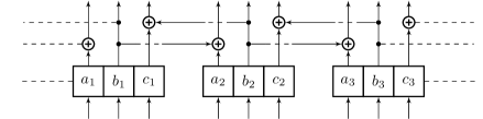
Figure 4: One-dimensional CA which is a not a QLGA after quantization

Define the global evolution $R$ on ${\mathcal{H}}_{{\mathcal{C}}}$ through its action by a controlled-NOT operation on the neighborhood cells as follows.

$$R:|a_{x}\rangle \mapsto|a_{x}+b_{x-1}\rangle$$

$$|b_{x}\rangle \mapsto|b_{x}\rangle$$

$$|c_{x}\rangle \mapsto|c_{x}+b_{x+1}\rangle$$

Let us write the element of Hadamard basis as: $|\chi_{a}\rangle=\frac{1}{\sqrt{2}}(|0\rangle+(-1)^{a}|1\rangle)$ for $a\in\mathbb{Z}/(2)$. Note that $|\chi_{0}\rangle=|+\rangle$ and $|\chi_{1}\rangle=|-\rangle$. We can equivalently look at the qubits in basis states: $|\chi_{a_{x}}\rangle\otimes|b_{x}\rangle\otimes|\chi_{c_{x}}\rangle$, where $a_{x},b_{x},c_{x}\in\mathbb{Z}/(2)$. Since $|+\rangle$ and $|-\rangle$ are eigenvectors of the shift operation with eigenvalues $1$ and $-1$ respectively, $R$ can be given as:

$$R:|\chi_{a_{x}}\rangle \mapsto|\chi_{a_{x}}\rangle$$

$$|b_{x}\rangle \mapsto{(-1)}^{b_{x}(a_{x+1}+c_{x-1})}|b_{x}\rangle$$

$$|\chi_{c_{x}}\rangle \mapsto|\chi_{c_{x}}\rangle$$

We now compute the subalgebras $\mathcal{D}_{{x-y},x}=\mathcal{R}_{x-y}\cap\mathcal{A}_{x}$, where $y\in\mathcal{N}$. $\mathcal{D}_{x,x}=\mathcal{R}_{x}\cap\mathcal{A}_{x}=\text{span}(\{|a_{x}\rangle\langle a_{x}|\otimes|b_{x}\rangle\langle b_{x}|\otimes|c_{x}\rangle\langle c_{x}|\})$, where $|a_{x}\rangle,|c_{x}\rangle\in\{|+\rangle,|-\rangle\}$, and $|b_{x}\rangle\in\{|0\rangle,|1\rangle\}$. $\mathcal{D}_{x-1,x}=\mathcal{R}_{x-1}\cap\mathcal{A}_{x}=\mathbb{C}\mathbb{I}\otimes\mathbb{I}\otimes\mathbb{I}$. $\mathcal{D}_{x+1,x}=\mathcal{R}_{x+1}\cap\mathcal{A}_{x}=\mathbb{C}\mathbb{I}\otimes\mathbb{I}\otimes\mathbb{I}$. Then it is clear that dim $\rm{span}(\prod_{y\in\{-1,0,1\}}\mathcal{D}_{{x-y},x})=8$, while dim $\mathcal{A}_{x}=64$. Theorem III.16 then implies that this QCA is not a QLGA.

The $2$-dimensional version of the above example is referred to as the Kari CA in Arrighi, Nesme, and Werner Arrighi et al. (2008). This is illustrated in Figure 5. The lattice $\mathcal{L}=\mathbb{Z}\times\mathbb{Z}$. A cell of this classical CA consists of $9$ bits. The neighborhood is $\mathcal{N}=\{-1,0,1\}\times\{-1,0,1\}$. The center bit of the center cell acts by controlled-NOT on the appropriate bit of the neighboring cell as shown.

Figure 5: Two-dimensional Kari CA which is a not a QLGA after quantization

In the quantized version, the cells of the QCA are $9$-qubits each. Enumerate the qubits of cell $x$ by $(i_{x},j_{x})\in\{-1,0,1\}\times\{-1,0,1\}$ (not to be confused with the neighborhood coordinates on the lattice). $(i_{x},j_{x})=(0,0)$ corresponds to the center qubit of a cell. The quiescent state is $|\hat{q}_{0}\rangle=\bigotimes_{(i_{x},j_{x})\in\{-1,0,1\}\times\{-1,0,1\}}|0\rangle$. The center qubit of the center cell acts by controlled-NOT on the appropriate qubit of the neighboring cell as for the classical CA. This action is exactly as in the $1$-dimensional case. The neighborhood is the same as for the classical CA, $\mathcal{N}=\{-1,0,1\}\times\{-1,0,1\}$.

We compute, as in the $1$-dimensional case, the subalgebras $\mathcal{D}_{{x-y},x}=\mathcal{R}_{x-y}\cap\mathcal{A}_{x}$, where $y\in\mathcal{N}$. $\mathcal{D}_{x,x}=\mathcal{R}_{x}\cap\mathcal{A}_{x}=\text{span}(\prod_{(i_{x},j_{x})\in\{-1,0,1\}\times\{-1,0,1\}}|a_{i_{x}j_{x}}\rangle\langle a_{i_{x}j_{x}}|)$, where $|a_{00}\rangle\in\{|0\rangle,|1\rangle\}$, and the rest of $|a_{i_{x}j_{x}}\rangle\in\{|+\rangle,|-\rangle\}$, for $(i_{x},j_{x})\neq(0,0)$. For all $y\in\mathcal{N}\setminus(0,0)$, $\mathcal{D}_{{x-y},x}=\mathcal{R}_{x-y}\cap\mathcal{A}_{x}=\mathbb{C}\bigotimes_{k\in\{-1,0,1\}\times\{-1,0,1\}}\mathbb{I}$. Then it is clear that dim $\rm{span}(\prod_{y\in\mathcal{N}}\mathcal{D}_{{x-y},x})=2^{9}$, while dim $\mathcal{A}_{x}=4^{9}$. Theorem III.16 then implies that this QCA is also not a QLGA.

IV.3 Examples of QCA that show effect of quantization on neighborhood

Consider a one-dimensional classical CA as in Figure 6 in which a cell is $2$ bits. We consider the scheme in which a cell $x$ is given by a pair $(a_{x},b_{x})$. The neighborhood is $\mathcal{N}=\{0,1\}$, and the update rule $\mu$:

$$\mu:a_{x} \mapsto a_{x}$$

$$b_{x} \mapsto b_{x}+a_{x}+a_{x+1}$$

Let us quantize this CA to get a QCA. A cell $x$ of the QCA consists of $2$ qubits: $|a_{x}\rangle\otimes|b_{x}\rangle$, where $a_{x},b_{x}\in\mathbb{Z}/(2)$. The quiescent state is $|\hat{q}_{0}\rangle=|0\rangle\otimes|0\rangle$. This automata is closely related to the “Toffoli CA” in Arrighi et al. (2008).

Define the global evolution $R$ on ${\mathcal{H}}_{{\mathcal{C}}}$ through its action by a controlled-NOT operation on the basis of its neighborhood.

$$R:|a_{x}\rangle \mapsto|a_{x}\rangle$$

$$|b_{x}\rangle \mapsto|b_{x}+a_{x}+a_{x+1}\rangle$$

The neighborhood looks like $\mathcal{N}_{+}=\{0,1\}$ as expected.

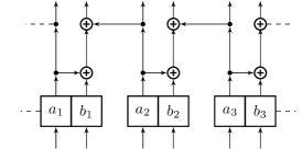
Figure 6: One-dimensional CA whose neighborhood changes after quantization

But we can equivalently look at the qubits in state: $|a_{x}\rangle\otimes|\chi_{b_{x}}\rangle$, where $a_{x},b_{x}\in\mathbb{Z}/(2)$, and $|\chi_{b_{x}}\rangle$ is as defined in the examples above: $|\chi_{b_{x}}\rangle=\frac{1}{\sqrt{2}}(|0\rangle+(-1)^{b_{x}}|1\rangle)$ for $b_{x}\in\mathbb{Z}/(2)$. Since $|\chi_{b_{x}}\rangle$ is an eigenvector for the shift operation, $R$ can be given as:

$$R:\quad\quad|a_{x}\rangle \mapsto{(-1)}^{a_{x}(b_{x-1}+b_{x})}|a_{x}\rangle$$

$$|\chi_{b_{x}}\rangle \mapsto|\chi_{b_{x}}\rangle$$

Now the neighborhood looks like $\mathcal{N}_{-}=\{-1,0\}$. In fact, the neighborhood is $\mathcal{N}=\mathcal{N}_{-}\cup\mathcal{N}_{+}=\{-1,0,1\}$. This is a consequence of the well-known fact that the control and target of a controlled-NOT operation in the basis $|+\rangle,|-\rangle$ are reversed as compared with the logical basis. Hence, while controlled-NOT operations can only propagate classical information in one direction (from control to target), they may propagate quantum information in both directions.

As before, we compute the subalgebras $\mathcal{D}_{{x-y},x}=\mathcal{R}_{x-y}\cap\mathcal{A}_{x}$, where $y\in\mathcal{N}$. $\mathcal{D}_{x,x}=\mathcal{R}_{x}\cap\mathcal{A}_{x}=\text{span}(\{|a_{x}\rangle\langle a_{x}|\otimes|b_{x}\rangle\langle b_{x}|\})$, where $|a_{x}\rangle\in\{|0\rangle,|1\rangle\}$, and $|b_{x}\rangle\in\{|+\rangle,|-\rangle\}$. $\mathcal{D}_{x-1,x}=\mathcal{R}_{x-1}\cap\mathcal{A}_{x}=\mathbb{C}\mathbb{I}\otimes\mathbb{I}$. $\mathcal{D}_{x+1,x}=\mathcal{R}_{x+1}\cap\mathcal{A}_{x}=\mathbb{C}\mathbb{I}\otimes\mathbb{I}$. Since dim $\rm{span}(\prod_{y\in\{-1,0,1\}}\mathcal{D}_{{x-y},x})=4$, while dim $\mathcal{A}_{x}=16$, Theorem III.16 implies that this QCA is again not a QLGA.

The change in neighborhood on quantization for this cellular automaton should lead us to question the original definition. Is there some redefinition of the cells that can maintain the same neighborhood for classical and quantum automata, and also yield a QLGA? We can in fact take the classical CA of Figure 6 and change it slightly by allowing a shift of bits, as shown in Figure 7. That is, we have an extra step that shifts the $a_{x+1}$ to $a_{x}$ before applying the add operation. The result is the following CA:

$$\mu:a_{x} \mapsto a_{x+1}$$

$$b_{x} \mapsto b_{x}+a_{x}+a_{x+1}$$

Then, after quantization, we obtain a QLGA from it. We accomplish that because the shift of bits corresponds to a shift of tensor factors (advection). This QLGA has a neighborhood $\mathcal{N}=\{0,1\}$, i.e., is a radius-$1/2$ QLGA.

$$R:|a_{x}\rangle \mapsto|a_{x+1}\rangle$$

$$|b_{x}\rangle \mapsto|b_{x}+a_{x}+a_{x+1}\rangle$$

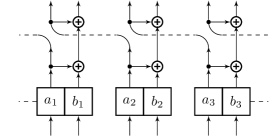
Figure 7: One-dimensional radius-$1/2$ QLGA from permutation of bits in the CA of Figure 6

V Conclusions

We have given a local algebraic condition for a quantum cellular automaton to be a quantum lattice-gas. This result classifies QLGA as a subset of QCA, and resolves the question of which QCA are equivalent to a circuit with a “brick structure”. This question has been open since Arrighi et al. Arrighi et al. (2008) produced an example showing that QLGA and QCA are distinct classes, contrary to the work of  Schumacher and Werner (2004). The question of classifying the remaining QCA that are not QLGA remains open. This open question motivates the reexamination of the definition of QCAs through local rules Watrous (1995); Durr et al. (1996); Dürr and Santha (2002); Meyer (1996c). The techniques introduced in this paper allow us to obtain rigorous results for models defined on the Hilbert space of finite, unbounded configurations. The definition of this space necessarily requires the definition of products with countably infinitely many terms von Neumann (1939); Guichardet (1972), just as is required for the constructions for WQCA defined through local rules Watrous (1995); Durr et al. (1996); Dürr and Santha (2002); Meyer (1996c). One might hope that the techniques that are used in the present paper may also have utility in deciding which quantum automata defined through local rules are also causal, and therefore true QCA.

Appendix A Some background and results on representations of associative algebras

We give a brief primer on representations of associative algebras relevant to this paper. The material in this section, except for Corollary A.6 and Theorem A.8, is drawn from the texts by Goodman and Wallach Goodman and Wallach (2009, 1999) and condensed for our purposes. Vector spaces in this section are assumed to be complex. A representation of an associative algebra $\mathcal{A}$ is a pair $(\gamma,V)$ such that $\gamma:\mathcal{A}\longrightarrow\text{End}(V)$ is an associative algebra isomorphism. Since a representation $(\gamma,V)$ of $\mathcal{A}$ makes $V$ an $\mathcal{A}$-module under the action: $av=\gamma(a)v$, for $a\in\mathcal{A}$, and $v\in V$, we can call $V$ an $\mathcal{A}$-module instead (with $\gamma$ implied by the context). If $U$ is a linear subspace of $V$ such that $\gamma(a)U\subset U$ for all $a\in\mathcal{A}$, then $U$ is invariant under the representation. A representation $(\gamma,V)$ is irreducible if the only invariant subspaces are $\{0\}$ and $V$.

Let $(\gamma,V)$, $(\mu,W)$ be two representations of an associative algebra $\mathcal{A}$. Let $\rm{Hom}(V,W)$ be the space of $\mathbb{C}$-linear maps from $V$ to $W$. Denote by $\rm{Hom}_{\mathcal{A}}(V,W)$ the set of all $T\in\rm{Hom}(V,W)$ such that $T\gamma(a)=\mu(a)T$ for all $a\in\mathcal{A}$. Such a map is called an intertwining operator between the two representations. Two representations $(\gamma,V)$, $(\mu,W)$ are equivalent if there exists an invertible intertwining operator between the two representations.

Lemma A.1 (Schur’s Lemma, Lemma $4.1.4$, pg. 180, Goodman and Wallach Goodman and Wallach (2009)).

Let $(\gamma,V)$ and $(\mu,W)$ be irreducible representations of an associative algebra $\mathcal{A}$. Assume that $V$ and $W$ have countable dimension over $\mathbb{C}$. Then

$$\rm{dim}\>\rm{Hom}_{\mathcal{A}}(V,W)=\left\{\begin{array}[]{lr}1,&\text{if }(\gamma,V)\cong(\mu,W)\\ 0,&\text{otherwise}\end{array}\right.$$

Let $(\gamma,V)$ be a finite-dimensional representation of $\mathcal{A}$. Let $\widehat{\mathcal{A}}$ be the set of all equivalence classes of finite-dimensional irreducible representations of $\mathcal{A}$. For each $\lambda\in\widehat{\mathcal{A}}$, fix a model $(\pi^{\lambda},V^{\lambda})$. Let:

$$U^{\lambda}=\rm{Hom}_{\mathcal{A}}(V^{\lambda},V)$$ (34)

For each $\lambda\in\widehat{\mathcal{A}}$, $U^{\lambda}$ is called a multiplicity space.

Define the map:

$$S_{\lambda}:U^{\lambda}\otimes V^{\lambda} \longrightarrow V$$ (35)

$$u^{\lambda}\otimes v^{\lambda} \mapsto u^{\lambda}(v^{\lambda})$$

Then $S_{\lambda}$ is an intertwining operator with $U^{\lambda}\otimes V^{\lambda}$ an $\mathcal{A}$-module under the action $a.(u\otimes v)=u\otimes(av)$ for $a\in\mathcal{A}$.

For $\lambda\in\widehat{\mathcal{A}}$, define the $\lambda$-isotypic component:

$$V^{[\lambda]}:\sum_{W\subset V:W\sim\lambda}W$$

A finite-dimensional $\mathcal{A}$-module $V$ is called completely reducible if for every invariant subspace $W\subset V$ there is a complementary invariant subspace $U$ such that $V=W\oplus U$. The following result (Proposition $4.1.11$, pg. 183, in Goodman and Wallach (2009)) provides equivalent characterizations of completely reducible representations.

Proposition A.2.

Let $(\gamma,V)$ be a finite-dimensional representation of $\mathcal{A}$. The following are equivalent:

1. $V$ is completely reducible.

2. $V=V_{1}\oplus\cdots\oplus V_{s}$ with each $V_{i}$ an irreducible $\mathcal{A}$-module.

3. $V=W_{1}+\cdots+W_{d}$ with each $W_{j}$ an irreducible $\mathcal{A}$-module.

Let $(\gamma,V)$ be a finite-dimensional representation of $\mathcal{A}$, such that $V$ is a completely reducible $\mathcal{A}$-module. Then it is a result from the representation theory of associative algebras (Goodman and Wallach Goodman and Wallach (1999), Proposition $3.1.6$, pg. $120$), that the map $S_{\lambda}$ in (35) is an $\mathcal{A}$-module isomorphism of $U^{\lambda}\otimes V^{\lambda}$ with the submodule $V^{[\lambda]}\subset V$:

$$U^{\lambda}\otimes V^{\lambda}\cong V^{[\lambda]}$$ (36)

Further:

$$V=\bigoplus_{\lambda\in\widehat{\mathcal{A}}}V^{[\lambda]}$$

This is called the primary decomposition of $V$. Thus if we extend the maps $S_{\lambda}$ as follows:

$$S_{\gamma}=\bigoplus_{\lambda\in\widehat{\mathcal{A}}}S_{\lambda}:\bigoplus_{\lambda\in\widehat{\mathcal{A}}}U^{\lambda}\otimes V^{\lambda} \longrightarrow V$$ (37)

$$\sum_{\lambda\in\widehat{\mathcal{A}}}u^{\lambda}\otimes v^{\lambda} \mapsto\sum_{\lambda\in\widehat{\mathcal{A}}}u^{\lambda}(v^{\lambda})$$

then $S_{\gamma}$ in (37) is an isomorphism of $\mathcal{A}$-modules (where $V$ is an $\mathcal{A}$-module via $\gamma$). Then we have the following isomorphism of algebras.

$$S_{\gamma}^{-1}\gamma(a)\ S_{\gamma}=\bigoplus_{\lambda\in\widehat{\mathcal{A}}}\mathbb{I}_{U^{\lambda}}\otimes\pi^{\lambda}(a)$$ (38)

where $a\in\mathcal{A}$, $U^{\lambda}$ is as in (34), and $(\pi^{\lambda},V^{\lambda})$ is a model for the class $\lambda$.

We state the Double Commutant Theorem, in Goodman and Wallach Goodman and Wallach (2009) pg. $184$, specialized here for a finite-dimensional vector space. Let $V$ be a finite-dimensional vector space. Define, for any subset $\mathcal{S}\subset\text{End}(V)$, the commutant of $\mathcal{S}$:

$$\text{Comm}(\mathcal{S})=\{y\in\text{End}(V):ys=sy\>\>\forall s\in\mathcal{S}\}$$ (39)

Theorem A.3 (Double Commutant, Theorem $4.1.13$ Goodman and Wallach (2009)).

Suppose $\mathcal{A}\subset\rm{End}(V)$ is a subalgebra containing the identity operator, such that $V$ is a completely reducible $\mathcal{A}$-module. Set $\mathcal{B}=\rm{Comm}(\mathcal{A})$. Then $\mathcal{A}=\rm{Comm}(\mathcal{B})$.

Denote by $\rm{Spec}(\gamma)$ the set of irreducible representations that occur in the primary decomposition of $V$. For each $\lambda\in\rm{Spec}(\gamma)$, the multiplicity space $U^{\lambda}=\rm{Hom}_{\mathcal{A}}(V_{\lambda},V)$ in (37) is a $\rm{Comm}(\mathcal{A})$-module under the action:

$$b.u=bu$$ (40)

where $b\in\rm{Comm}(\mathcal{A})$, and $u\in U^{\lambda}$, and $bu:V^{\lambda}\underrightarrow{u}V\underrightarrow{b}V$ is the composition (left multiplication by $b$) map.

We adapt some results from Goodman and Wallach Goodman and Wallach (2009), Section $4.2.1$ (General Duality Theorem). Except for some substitutions, these results are taken exactly as in the said reference, including the proofs. We obtain from the originals, derived in the setting of group representations, the versions relevant to subalgebras of $\rm{End}(V)$. Thus we get the associative algebra counterparts of the Duality Theorem, Theorem $4.2.1$ Goodman and Wallach (2009), and Corollary $4.2.4$ in Goodman and Wallach (2009).

Theorem A.4 (Duality, Theorem $4.2.1$ Goodman and Wallach (2009)).

Suppose $\mathcal{A}\subset\rm{End}(V)$ is an subalgebra containing the identity operator. Let $V$ be a completely reducible $\mathcal{A}$-module. Each multiplicity space $U^{\lambda}$ in (37) is an irreducible $\rm{Comm}(\mathcal{A})$-module. Furthermore, if $\lambda,\mu\in\widehat{\mathcal{A}}$, and $U^{\lambda}\cong U^{\mu}$ as $\rm{Comm}(\mathcal{A})$-module, then $\lambda=\mu$.

Proof.

We first prove that the action of $\rm{Comm}(\mathcal{A})$ on $U^{\lambda}$ is irreducible. Let $T\in U^{\lambda}$ be nonzero. Given another nonzero element $S\in U^{\lambda}$ we need to find $r\in\rm{Comm}(\mathcal{A})$ such that $rT=S$. Let $X=TV^{\lambda}$ and $Y=SV^{\lambda}$. Then by Schur’s Lemma (Lemma A.1), $X$ and $Y$ are isomorphic $\mathcal{A}$-modules of class $\lambda$. Thus there exists $u\in\rm{Comm}(\mathcal{A})$ such that $uT:V^{\lambda}\longrightarrow SV^{\lambda}$ is an $\mathcal{A}$-module isomorphism. Schur’s Lemma implies that there exists $c\in\mathbb{C}$ such that $cuT=S$, so we may take $r=cu$.

We now show that if $\lambda\neq\mu$ then $U^{\lambda}$ and $U^{\mu}$ are inequivalent modules for $\rm{Comm}(\mathcal{A})$. Suppose

$$\phi:U^{\lambda}\longrightarrow U^{\mu}$$

is an intertwining operator for the action of $\rm{Comm}(\mathcal{A})$. Let $T\in U^{\lambda}$ be nonzero and set $S=\phi(T)$. We want to show that $S=0$. Set $U=TV^{\lambda}+SV^{\mu}$. Then since we are assuming $\lambda\neq\mu$, the sum is direct. Let $p:U\longrightarrow SV^{\mu}$ be the corresponding projection. Then $p\in\rm{Comm}(\mathcal{A})$. Since $pT=0$, we have:

$$0=\phi(pT)=p\phi(T)=pS=S\text{,}$$

which proves that $\phi=0$. ∎

Corollary A.5 (Corollary $4.2.4$ Goodman and Wallach (2009)).

Let $\mathcal{B}=\rm{Comm}(\mathcal{A})$. Then $V$ is a completely reducible $\mathcal{B}$-module. Furthermore, the following hold:

1. Suppose for every $\lambda\in\rm{Spec}(\gamma)$ there is given an operator $T_{\lambda}\in\rm{End}(V^{\lambda})$. Then there exists $T\in\mathcal{A}$ that acts by $\mathbb{I}\otimes T_{\lambda}$ on the $\lambda$-summand in the decomposition (37).

2. Let $T\in\mathcal{A}\cap\mathcal{B}$ (the center of $\mathcal{A}$). Then $T$ is diagonalized by (37) and acts by scalar ${\hat{T}}(\lambda)\in\mathbb{C}$ on $U^{\lambda}\otimes V^{\lambda}$. Conversely, given any complex valued function $f$ on $\rm{Spec}(\gamma)$, there exists $T\in\mathcal{A}\cap\mathcal{B}$ such that ${\hat{T}}(\lambda)=f(\lambda)$.

Proof.

Since $V$ is the direct sum of $\mathcal{B}$-invariant irreducible subspaces by Theorem A.4, it is a completely reducible $\mathcal{B}$-module by Proposition A.2. We now prove the other assertions.

1. Let $T\in\rm{End}(V)$ be the operator that acts by $\mathbb{I}\otimes T_{\lambda}$ on the $\lambda$ summand. Then $T\in\rm{Comm}(\mathcal{B})$, and hence $T\in\mathcal{A}$ by the Double Commutant Theorem (Theorem A.3).

2. Each summand in (37) is invariant under $T$, and the action of $T$ on the $\lambda$ summand is by an operator of the form $R_{\lambda}\otimes\mathbb{I}=\mathbb{I}\otimes S_{\lambda}$ with $R_{\lambda}\in\rm{End}(U^{\lambda})$, and $S_{\lambda}\in\rm{End}(V^{\lambda})$. Such an operator must be a scalar multiple of the identity operator. The converse follows from (i).

∎

An algebra $\mathcal{B}$ is simple if the only two sided ideals in $\mathcal{B}$ are $0$ and $\mathcal{B}$. An algebra $\mathcal{A}$ is a semisimple algebra if it is a finite direct sum of simple algebras. This is equivalent, by Wedderburn’s Theorem (Goodman and Wallach Goodman and Wallach (1999), Theorem $3.2.1$, pg. $128$), to the statement that $\mathcal{A}$ is isomorphic to a finite sum of matrix algebras.

For an algebra $\mathcal{A}\subset\rm{End}(V)$, such that $V$ is a completely reducible $\mathcal{A}$-module, let $\rm{Spec}(\mathcal{A})$ be the set of irreducible representations that occur in the primary decomposition of $V$.

Corollary A.6.

Let $\mathcal{A}\subset\rm{End}(V)$ be a subalgebra containing the identity operator, such that $V$ is a completely reducible $\mathcal{A}$-module. Let $\mathcal{B}=\rm{Comm}(\mathcal{A})$. Then there is an $\mathcal{A}$-module isomorphism:

$$S_{V}:\bigoplus_{\lambda\in\widehat{\mathcal{A}}}U^{\lambda}\otimes V^{\lambda} \longrightarrow V$$ (41)

$$\sum_{\lambda\in\widehat{\mathcal{A}}}u^{\lambda}\otimes v^{\lambda} \mapsto\sum_{\lambda\in\widehat{\mathcal{A}}}u^{\lambda}(v^{\lambda})$$

where $V^{\lambda}$ is an irreducible module for the class $\lambda\in\widehat{\mathcal{A}}$, and $U^{\lambda}=\rm{Hom}_{\mathcal{A}}(V^{\lambda},V)$. Under this isomorphism:

$$\mathcal{A}\cong\bigoplus_{\lambda\in\widehat{\mathcal{A}}}\mathbb{I}_{U^{\lambda}}\otimes\rm{End}(V^{\lambda})$$

and:

$$\mathcal{B}\cong\bigoplus_{\lambda\in\widehat{\mathcal{A}}}\rm{End}(U^{\lambda})\otimes\mathbb{I}_{V^{\lambda}}$$

where the action of $\mathcal{B}$ on each $U^{\lambda}$ is given by (40).

In particular, $\mathcal{A}$ is semisimple.

Proof.

$V$ is a completely reducible $\mathcal{A}$-module. This implies there is an $\mathcal{A}$-module isomorphism given by (37):

$$S_{V}:\bigoplus_{\lambda\in\widehat{\mathcal{A}}}U^{\lambda}\otimes V^{\lambda} \longrightarrow V$$

$$\sum_{\lambda\in\widehat{\mathcal{A}}}u^{\lambda}\otimes v^{\lambda} \mapsto\sum_{\lambda\in\widehat{\mathcal{A}}}u^{\lambda}(v^{\lambda})$$

where $V^{\lambda}$ is an irreducible module for the class $\lambda\in\widehat{\mathcal{A}}$, and $U^{\lambda}=\rm{Hom}_{\mathcal{A}}(V^{\lambda},V)$. Then by definition of $\mathcal{A}$ action (as a subalgerba of $\rm{End}(V)$) on $V$, under this isomorphism, Corollary A.5 implies:

$$\mathcal{A}\cong\bigoplus_{\rm{Spec}(\mathcal{A})}\mathbb{I}_{U^{\lambda}}\otimes\rm{End}(V^{\lambda})$$

Since $V$ is finite-dimensional, the above implies that $\rm{Spec}(\mathcal{A})$ is a finite set. This in turn implies that $\mathcal{A}$ is semisimple as it is isomorphic to a finite direct sum of finite dimensional matrix algebras. Then a standard theorem on semisimple algebras, Proposition $3.3.1$ in Goodman and Wallach (1999), implies that each irreducible representations of $\mathcal{A}$ is equivalent to some element of $\rm{Spec}(\mathcal{A})$. Hence $\widehat{\mathcal{A}}=\rm{Spec}(\mathcal{A})$. Therefore:

$$\mathcal{A}\cong\bigoplus_{\lambda\in\widehat{\mathcal{A}}}\mathbb{I}_{U^{\lambda}}\otimes\rm{End}(V^{\lambda})$$

By Duality Theorem (Theorem A.4), under $S_{V}$:

$$\mathcal{B}\cong\bigoplus_{\lambda\in\widehat{\mathcal{A}}}\rm{End}(U^{\lambda})\otimes\mathbb{I}_{V^{\lambda}}$$

where the action of $\mathcal{B}$ on each $U^{\lambda}$ is given by (40). ∎

We state the semisimple algebra version of the Double Commutant Theorem, in Goodman and Wallach Goodman and Wallach (1999) pg. $137$.

Theorem A.7 (Double Commutant Theorem for Semisimple Algebras).

Suppose $\mathcal{A}\subset\rm{End}(V)$ is a semisimple subalgebra containing the identity operator. Then the algebra $\mathcal{B}=\rm{Comm}(\mathcal{A})$ is semisimple and $\mathcal{A}=\rm{Comm}(\mathcal{B})$. Furthermore, there exists an $\mathcal{A}$-module isomorphism:

$$S_{\mathcal{A}}:\bigoplus^{r}_{j=1}U_{j}\otimes V_{j} \longrightarrow V$$

$$\sum^{r}_{j=1}u_{j}\otimes v_{j} \mapsto\sum^{r}_{j=1}u_{j}(v_{j})$$

where $V_{j}$ is an irreducible $\mathcal{A}$-module, and $U_{j}=\rm{Hom}_{\mathcal{A}}(V_{j},V)$. Under this isomorphism:

$$\mathcal{A}\cong\bigoplus^{r}_{j=1}\mathbb{I}_{U_{j}}\otimes\rm{End}(V_{j})$$

and:

$$\mathcal{B}\cong\bigoplus^{r}_{j=1}\rm{End}(U_{j})\otimes\mathbb{I}_{V_{j}}$$

Next we consider a general Hilbert space, and state the remarkable von Neumann Density Theorem. The proof of the von Neumann Density Theorem can be found in Kadison and Ringrose (1983); Wallach (1992). Consider a Hilbert space $\mathcal{H}$ and the space, $B(\mathcal{H})$, of bounded linear operators of $\mathcal{H}$. Recall the following definition. For any subset $\mathcal{S}\subset B(\mathcal{H})$, the commutant of $\mathcal{S}$ is defined as:

$$\text{Comm}(\mathcal{S})=\{y\in B(\mathcal{H}):ys=sy\>\>\forall s\in\mathcal{S}\}$$

Theorem A.8 (von Neumann Density Theorem).

Let $\mathcal{A}\subset B(\mathcal{H})$ be a self-adjoint algebra of operators containing the identity operator, then the weak and strong closures of $\mathcal{A}$ in $B(\mathcal{H})$ is $\rm{Comm}(\rm{Comm}(\mathcal{A}))$.

Appendix B Some results on representations of self-adjoint algebras

We state a few results on representations of self-adjoint algebras. Let $V$ be a finite-dimensional Hilbert space, with an inner product $\langle\cdot|\cdot\rangle$, and $\mathcal{A}\subset\rm{End}(V)$ a subalgebra. Let the adjoint of an algebra $\mathcal{A}\subset\rm{End}(V)$ be $\mathcal{A}^{\dagger}=\{A^{\dagger}:A\in\mathcal{A}\}$. An algebra $\mathcal{A}$ is self-adjoint if $\mathcal{A}=\mathcal{A}^{\dagger}$. From the results in this section, Lemma B.1, and Proposition B.2 appear in Procesi (2007) (pg. 145).

Lemma B.1.

Let $\mathcal{A}\subset\rm{End}(V)$ be a self-adjoint subalgebra. If $W\in V$ is an $\mathcal{A}$-invariant subspace, then $W^{\perp}=\{{v}\in V:\langle v|w\rangle=0\>\forall\>{w}\in W\}$ is $\mathcal{A}$-invariant.

Proof.

Let ${w}\in W$, ${v}\in W^{\perp}$, $A\in\mathcal{A}$. Then $A^{\dagger}\in\mathcal{A}$, which implies $A^{\dagger}{w}\in W$ $\implies$ $\langle A{v}|w\rangle=\langle v|A^{\dagger}w\rangle=0$ $\implies$ $A{v}\in W^{\perp}$. ∎

Proposition B.2.

Let $\mathcal{A}\subset\rm{End}(V)$ be a self-adjoint subalgebra. Then $V$ is an orthogonal direct sum of irreducible $\mathcal{A}$-modules. In particular, $V$ is a completely reducible $\mathcal{A}$-module.

Proof.

Let $W\subset V$ be an $\mathcal{A}$-invariant subspace of minimal dimension. Then it is by definition irreducible. Since $\mathcal{A}=\mathcal{A}^{\dagger}$, by Lemma B.1, $V=W\oplus W^{\perp}$ is an orthogonal direct sum of $\mathcal{A}$-modules. The conclusion follows by induction on dimension. ∎

Corollary B.3.

Let $\mathcal{A}\subset\rm{End}(V)$ be a self-adjoint subalgebra containing the identity operator. Then $\mathcal{A}$ is semisimple.

Proof.

By Proposition B.2, $V$ is a completely reducible $\mathcal{A}$-module. Then Corollary A.6 implies that $\mathcal{A}$ is semisimple. ∎

Corollary B.4.

Let $\mathcal{A}\subset\rm{End}(V)$ be a self-adjoint subalgebra. Then there exist for every $\lambda\in\widehat{\mathcal{A}}$, a set of intertwining operators $\{u^{\lambda}_{j}\}\subset U^{\lambda}$, such that the $\lambda$-isotypic component can be written as an orthogonal direct sum: $V^{[\lambda]}=\bigoplus_{j}u^{\lambda}_{j}(V^{\lambda})$.

Proof.

By Proposition B.2, $V$ is a completely reducible $\mathcal{A}$-module. Thus by (36), $S_{\lambda}$ in (35) is an $\mathcal{A}$-module isomorphism:

$$S_{\lambda}:U^{\lambda}\otimes V^{\lambda}\longrightarrow V^{[\lambda]}$$

Again by Proposition B.2, the $\lambda$-isotypic component,

$$V^{[\lambda]}=\bigoplus_{W_{j}\subset V:W_{j}\sim\lambda}W_{j}$$

is an orthogonal direct sum. Choose $u_{j}$ such that $u_{j}(V^{\lambda})=W_{j}$. ∎

Appendix C Structural Reversibility

We prove the Structural Reversibility (due to Arrighi, Nesme, and Werner Arrighi et al. (2008)), in our context, to make the present paper self-contained.

Theorem C.1 (Structural Reversibility ).

Let $M:\mathcal{H}_{\mathcal{C}}\longrightarrow\mathcal{H}_{\mathcal{C}}$ be a unitary operator and $\mathcal{N}$ a neighborhood. Let $\mathcal{V}=\{-k|k\in\mathcal{N}\}$. Then the following are equivalent:

1. $M$ is causal relative to the neighborhood $\mathcal{N}$.

2. For every operator $A_{x}$ local upon cell $x$, $M^{\dagger}A_{x}M$ is local upon $\mathcal{N}_{x}$.

3. $M^{\dagger}$ is causal relative to the neighborhood $\mathcal{V}$.

4. For every operator $A_{x}$ local upon cell $x$, $MA_{x}M^{\dagger}$ is local upon ${\mathcal{V}}_{x}$.

Before proving the theorem, we prove the following lemma:

Lemma C.2.

Denote the set of density operators on $\mathcal{H}_{\mathcal{C}}$ by $\Omega$. For $A\in B(\mathcal{H}_{\mathcal{C}})$, define the map:

$$f_{A}:\Omega\longrightarrow\mathbb{C}$$

$$f_{A}(\rho)=\rm{tr}(A\rho)$$

where $\rm{tr}$ is the trace operator. Let $D\in\mathbb{Z}^{n}$ be a finite subset. Then:

1. $A$ is local upon $D$ if and only if for every pair $\rho,\rho^{\prime}\in\Omega$ satisfying $\rho_{|_{D}}={\rho^{\prime}}_{|_{D}}$, $f_{A}(\rho)=f_{A}(\rho^{\prime})$.

2. $\rho,\rho^{\prime}\in\Omega$ satisfy $\rho_{|_{D}}={\rho^{\prime}}_{|_{D}}$, if and only if for every $A$ local upon $D$, $f_{A}(\rho)=f_{A}(\rho^{\prime})$.

Proof.

For elements of $B(\mathcal{H}_{\mathcal{C}})$ that are local on some finite subset $K\subset\mathbb{Z}^{n}$, by abuse of notation, we call both $B\in\mathcal{Z}$ ($\mathcal{Z}$ as in (8)) and $\iota^{-1}_{K}(B)$ ($\iota_{K}$ as in (7)) by $B$.

(i) Suppose $A$ is local upon $D$ and $\rho,\rho^{\prime}\in\Omega$ are such that $\rho_{|_{D}}={\rho^{\prime}}_{|_{D}}$. Then $f_{A}(\rho)=\rm{tr}(A\rho)=\rm{tr}(A\rho_{|_{D}})=\rm{tr}(A{\rho^{\prime}}_{|_{D}})=\text{tr}(A\rho^{\prime})=f_{A}(\rho^{\prime})$.

For the converse, suppose $A$ is not local upon $D$. We can choose an orthonormal basis $\{|v_{j}\rangle\}$ for $\bigotimes_{k\in D}W$. Then we can write (special case of  (6)):

$$A=\sum_{(l,m)}|v_{l}\rangle\langle v_{m}|\otimes A_{l,m}$$

where $\{(l,m)\}\subset\{1,\ldots,d_{W}\}\times\{1,\ldots,d_{W}\}$, and $A_{l,m}\in B(\mathcal{H}_{\mathcal{C}_{\overline{D}}})$ are non-zero. Since $A$ is not local upon $D$, not all the $A_{l,m}$ are multiples of the identity, $\mathbb{I}_{\overline{D}}$, on $\mathcal{H}_{\mathcal{C}_{\overline{D}}}$. There are two cases to consider:

1. There is an $A_{l,l}$ for some $l$ such that $A_{l,l}$ is not a multiple of $\mathbb{I}_{\overline{D}}$. Then there exist two unit vectors $|x\rangle,|y\rangle\in\mathcal{H}_{\mathcal{C}_{\overline{D}}}$, such that $\langle x|A_{l,l}|x\rangle\neq\langle y|A_{l,l}|y\rangle$. Let $\rho=|v_{l}\rangle\langle v_{l}|\otimes|x\rangle\langle x|,\rho^{\prime}=|v_{l}\rangle\langle v_{l}|\otimes|y\rangle\langle y|$. Then $\rho_{|_{D}}={\rho^{\prime}}_{|_{D}}$ whereas $f_{A}(\rho)\neq f_{A}(\rho^{\prime})$.

2. Every $A_{l,l}$ is a multiple of $\mathbb{I}_{\overline{D}}$. Then choose some $A_{l,m}$ which is not. Then there exist two unit vectors $|x\rangle,|y\rangle\in\mathcal{H}_{\mathcal{C}_{\overline{D}}}$, such that $\langle x|A_{l,m}|x\rangle\neq\langle y|A_{l,m}|y\rangle$. Let $\rho=(|v_{l}\rangle\langle v_{l}|+|v_{l}\rangle\langle v_{m}|)\otimes|x\rangle\langle x|,\rho^{\prime}=(|v_{l}\rangle\langle v_{l}|+|v_{l}\rangle\langle v_{m}|)\otimes|y\rangle\langle y|$. Then $\rho_{|_{D}}={\rho^{\prime}}_{|_{D}}$ whereas $f_{A}(\rho)\neq f_{A}(\rho^{\prime})$.

(ii) Suppose $A$ is local upon $D$ and $\rho,\rho^{\prime}\in\Omega$ are such that $\rho_{|_{D}}={\rho^{\prime}}_{|_{D}}$. Then $f_{A}(\rho)=\rm{tr}(A\rho)=\rm{tr}(A\rho_{|_{D}})=\rm{tr}(A{\rho^{\prime}}_{|_{D}})=\text{tr}(A\rho^{\prime})=f_{A}(\rho^{\prime})$.

For the converse, let $\rho,\rho^{\prime}\in\Omega$, such that for all $A$ local upon $D$, $f_{A}(\rho)=f_{A}({\rho^{\prime}})$. Consider $A=|v_{l}\rangle\langle v_{m}|\otimes\mathbb{I}_{\overline{D}}$, a basis element of operators local upon $D$. Then $f_{A}(\rho)=\langle v_{m}|\rho_{|_{D}}|v_{l}\rangle$, $f_{A}(\rho^{\prime})=\langle v_{m}|{\rho^{\prime}}_{|_{D}}|v_{l}\rangle$. This implies by $f_{A}(\rho)=f_{A}({\rho^{\prime}})$, that $\langle v_{m}|\rho_{|_{D}}|v_{l}\rangle=\langle v_{m}|{\rho^{\prime}}_{|_{D}}|v_{l}\rangle$. Since this is true for all elements of $\{|v_{l}\rangle\langle v_{m}|:1\leq l,m\leq d_{W}\}$, i.e., for a set of basis elements of operators local upon $D$, then by linearity, $\rho_{|_{D}}={\rho^{\prime}}_{|_{D}}$.

∎

Proof of Theorem C.1.

Note:

$$\text{tr}(M\rho M^{\dagger}A)=\text{tr}(\rho M^{\dagger}AM):\>\ \forall\rho\in\Omega$$ (42)

$~{}\ref{strv1}\implies~{}\ref{strv2}$ Let $M$ be causal. Suppose $\rho$ and $\rho^{\prime}$ is a pair such that $\rho|_{\mathcal{N}_{x}}={\rho^{\prime}}|_{\mathcal{N}_{x}}$, and $A$ is local upon $x$. Causality implies $\text{tr}(M\rho M^{\dagger}A)=\text{tr}(M{\rho^{\prime}}M^{\dagger}A)$. By (42), $\text{tr}(\rho M^{\dagger}AM)=\text{tr}({\rho^{\prime}}M^{\dagger}AM)$, so by Lemma C.2 (i), $M^{\dagger}AM$ is local upon $\mathcal{N}_{x}$.

$~{}\ref{strv2}\implies~{}\ref{strv1}$ Suppose $A$ is local upon $x$, $\rho$ and $\rho^{\prime}$ be a pair of density operators such that $\rho|_{\mathcal{N}_{x}}={\rho^{\prime}}|_{\mathcal{N}_{x}}$, and $M^{\dagger}AM$ is local upon $\mathcal{N}_{x}$. Then $\text{tr}(\rho M^{\dagger}AM)=\text{tr}({\rho^{\prime}}M^{\dagger}AM)$. By (42), $\text{tr}(M\rho M^{\dagger}A)=\text{tr}(M{\rho^{\prime}}M^{\dagger}A)$, so by Lemma C.2 (ii), $M\rho M^{\dagger}|_{x}=M{\rho^{\prime}}M^{\dagger}|_{x}$.

$~{}\ref{strv2}\implies~{}\ref{strv4}$ Suppose $A_{x}$ is local upon $x$. Let $A_{y}$ be an operator local upon $y\notin{\mathcal{V}}_{x}$. Then $M^{\dagger}A_{y}M$ is local upon $\mathcal{N}_{y}$. But $x\notin\mathcal{N}_{y}$, so $M^{\dagger}A_{y}M$ commutes with $A_{x}$. But then $A_{y}=MM^{\dagger}A_{y}MM^{\dagger}$ commutes with $MA_{x}M^{\dagger}$, by the definition of conjugation. This applies to every $A_{y}\in\mathcal{A}_{y}$, hence $MA_{x}M^{\dagger}$ commutes with $\mathcal{A}_{y}$. We can express $MA_{x}M^{\dagger}$ as a finite sum (as in (6)):

$$MA_{x}M^{\dagger}=\sum_{l}e_{l}\otimes E_{l}$$ (43)

where $\{e_{l}\}\subset\text{End}(\bigotimes_{k\in\mathcal{V}_{x}}W)$ ia a linearly independent set, and $E_{l}\in B(\mathcal{H}_{\mathcal{C}_{\overline{\mathcal{V}_{x}}}})$ (the space of bounded linear operators on the co-$\mathcal{V}_{x}$ space, $\mathcal{H}_{\mathcal{C}_{\overline{\mathcal{V}_{x}}}}$, defined in Definition III.1, with $D=\mathcal{V}_{x}$).

For any $B\in\text{End}(\bigotimes_{k\in\mathcal{V}_{x}}W)$, $B\otimes\mathbb{I}_{\overline{\mathcal{V}_{x}}}$ (where $\mathbb{I}_{\overline{\mathcal{V}_{x}}}$ is the identity on $\mathcal{H}_{\mathcal{C}_{\overline{\mathcal{V}_{x}}}}$) also commutes with $A_{y}$, This implies $(B\otimes\mathbb{I}_{\overline{\mathcal{V}_{x}}})(MA_{x}M^{\dagger})$ commutes with $A_{y}$. Using the standard commutator notation $[.,.]$ ([X,Y]=XY-YX), we write:

$$[A_{y},(B\otimes\mathbb{I}_{\overline{\mathcal{V}_{x}}})(MA_{x}M^{\dagger})]=\sum_{l}(Be_{l})\otimes[A_{y},E_{l}]=0$$

We can trace out the finite dimensional part. Let the operator thus obtained on $\mathcal{H}_{\mathcal{C}_{\overline{\mathcal{V}_{x}}}}$ be $\zeta(B)$:

$$\zeta(B)=\sum_{l}\text{tr }(Be_{l})[A_{y},E_{l}]=\sum_{l}\text{tr }(Be_{l})[A_{y},E_{l}]=0$$

Since $(X,Y)=\text{tr}(XY)$ is a nondegenerate bilinear form on $\text{End}(\bigotimes_{k\in\mathcal{V}_{x}}W)$, and $\{e_{l}\}$ is a linearly independent set, we can choose a set $\{B_{l}\}\subset\text{End}(\bigotimes_{k\in\mathcal{V}_{x}}W)$ (indexed by the same set $\{l\}$ that indexes $\{e_{l}\}$) such that $\text{tr }(B_{k}e_{l})=\delta_{k,l}$. Then:

$$\zeta(B_{k})=[A_{y},E_{k}]=0$$ (44)

The subalgebra of $B(\mathcal{H}_{\mathcal{C}_{\overline{\mathcal{V}_{x}}}})$ generated by $\mathcal{A}_{y}$, $y\notin\mathcal{V}_{x}$ acts irreducibly on the space $\mathcal{H}_{\mathcal{C}_{\overline{\mathcal{V}_{x}}}}$ (by the argument in the proof of Theorem III.7, i.e., it acts transitively on a dense subspace, $\text{span}({\mathcal{C}}_{\overline{\mathcal{V}_{x}}})$, of $\mathcal{H}_{\mathcal{C}_{\overline{\mathcal{V}_{x}}}}$). By (44), $E_{k}$ commutes with this subalgebra. Schur’s Lemma (Lemma A.1) then implies that $E_{k}=\eta_{k}\mathbb{I}_{\overline{\mathcal{V}_{x}}}$ for some $\eta_{k}\in\mathbb{C}$. This is true for every $k\in\{l\}$. By (43):

$$MA_{x}M^{\dagger}=(\sum_{l}\eta_{l}e_{l})\otimes\mathbb{I}_{\overline{\mathcal{V}_{x}}}=a_{\mathcal{V}_{x}}\otimes\mathbb{I}_{\overline{\mathcal{V}_{x}}}$$

for some $a_{\mathcal{V}_{x}}\in\text{End}(\bigotimes_{k\in\mathcal{V}_{x}}W)$. Hence $MA_{x}M^{\dagger}$ is local upon ${\mathcal{V}}_{x}$.

$~{}\ref{strv4}\implies~{}\ref{strv2}$ Same argument as for the proof of $~{}\ref{strv2}\implies~{}\ref{strv4}$, except interchanging the roles of $\mathcal{N}_{x}$ and $\mathcal{V}_{x}$, $M$ and $M^{\dagger}$.

$~{}\ref{strv3}\iff~{}\ref{strv4}$ Same arguments as for the proof of $~{}\ref{strv1}\iff~{}\ref{strv2}$, except replacing $\mathcal{N}$ with $\mathcal{V}$, $\mathcal{N}_{x}$ with $\mathcal{V}_{x}$, and $M$ with $M^{\dagger}$. ∎

Appendix D Proof of Lemma III.15 requiring quiescent symbol $|\hat{q}_{0}\rangle$ to be an invariant of $F$

Lemma (Lemma III.15).

$\hat{F}$ is defined on $\hat{\mathcal{C}}$ as a map $\hat{F}:\hat{\mathcal{C}}\longrightarrow{\mathcal{H}}_{\hat{\mathcal{C}}}$, and can be extended to ${\mathcal{H}}_{\hat{\mathcal{C}}}$ as unitary and translation-invariant operator, if and only if $F$ has $|\hat{q}_{0}\rangle$ as an invariant (an eigenvector with eigenvalue one): $F|\hat{q}_{0}\rangle=|\hat{q}_{0}\rangle$.

Proof of Lemma III.15.

Let us assume that $\hat{F}$ is defined on $\hat{\mathcal{C}}$ as a map $\hat{F}:\hat{\mathcal{C}}\longrightarrow{\mathcal{H}}_{\hat{\mathcal{C}}}$, and can be extended to ${\mathcal{H}}_{\hat{\mathcal{C}}}$ as a unitary and translation-invariant operator. Then Lemma III.5 implies:

$$\hat{F}\big{(}\bigotimes_{x\in\mathbb{Z}^{n}}|\hat{q}_{0}\rangle\big{)}=\bigotimes_{x\in\mathbb{Z}^{n}}F|\hat{q}_{0}\rangle=e^{i\Theta_{0}}\bigotimes_{x\in\mathbb{Z}^{n}}|\hat{q}_{0}\rangle$$

for some $\Theta_{0}\in\mathbb{R}$. This implies, $F|\hat{q}_{0}\rangle=|\hat{q}_{0}\rangle$.

For the converse, assume $F|\hat{q}_{0}\rangle=|\hat{q}_{0}\rangle$. Then for every element $|\hat{c}\rangle=\bigotimes_{x\in\mathbb{Z}^{n}}|{\hat{c}}_{x}\rangle\in\hat{\mathcal{C}}$, under the formal definition of $\hat{F}$ in (26), $\hat{F}|\hat{c}\rangle=\bigotimes_{x\in\mathbb{Z}^{n}}F|{\hat{c}}_{x}\rangle\in{\mathcal{H}}_{\hat{\mathcal{C}}}$. Furthermore, as a map $\hat{F}:\hat{\mathcal{C}}\longrightarrow{\mathcal{H}}_{\hat{\mathcal{C}}}$, $\hat{F}$ preserves the inner product (since $F$ is a unitary operator on $\hat{W}=\bigotimes_{z\in\mathcal{N}}V_{z}$), and is translation-invariant, by the same definition. Then $\hat{F}$ can be extended to a unitary and translation-invariant operator on ${\mathcal{H}}_{\hat{\mathcal{C}}}$. ∎

References

- Aharonov et al. (1993) Aharonov, Y., Davidovich, L., and Zagury, N. (1993). Quantum random walks. Phys. Rev. A, 48, 1687–1690.
- Arrighi (2006) Arrighi, P. (2006). Algebraic characterizations of unitary linear quantum cellular automata. In R. Kralovic and P. Urzyczyn, editors, Mathematical Foundations of Computer Science 2006, volume 4162 of Lecture Notes in Computer Science, pages 122–133. Springer Berlin Heidelberg.
- Arrighi et al. (2008) Arrighi, P., Nesme, V., and Werner, R. (2008). One-dimensional quantum cellular automata over finite, unbounded configurations. In C. Martin-Vide, F. Otto, and H. Fernau, editors, Language and Automata Theory and Applications, volume 5196 of Lecture Notes in Computer Science, pages 64–75. Springer Berlin Heidelberg.
- Arrighi et al. (2011) Arrighi, P., Nesme, N., and Werner, R. (2011). Unitarity plus causality implies localizability. J. Comput. Syst. Sci., 77, 372–37.
- Aspuru-Guzik et al. (2005) Aspuru-Guzik, A., Dutoi, A. D., Love, P. J., and Head-Gordon, M. (2005). Simulated quantum computation of molecular energies. Science, 309, 1704.
- Beckman et al. (2001) Beckman, D., Gottesman, D., Nielsen, M. A., and Preskill, J. (2001). Causal and localizable quantum operations. Phys. Rev. A, 64, 052309.
- Boghosian and Taylor (1997) Boghosian, B. and Taylor, W. (1997). Quantum lattice-gas models for the many-body Schrödinger equation. International Journal of Modern Physics C, 8(4), 705–716.
- Boghosian and Taylor (1998a) Boghosian, B. and Taylor, W. (1998a). Quantum lattice-gas model for the many-particle Schrödinger equation in d dimensions. Phys Rev E, 57(1), 54–66.
- Boghosian and Taylor (1998b) Boghosian, B. and Taylor, W. (1998b). Simulating quantum mechanics on a quantum computer. Physica D, 120(1-2), 30–42.
- Boghosian et al. (2000) Boghosian, B. M., Coveney, P. V., and Love, P. J. (2000). A three-dimensional lattice gas model for amphiphilic fluid dynamics. Proc. Roy. Soc. London A., 456, 1431.
- Cheung and Perez-Delgado (2007) Cheung, D. and Perez-Delgado, A. (2007). Local unitary quantum cellular automata. Phys. Rev. A, 76, 032320.
- Childs et al. (1993) Childs, A. M., Farhi, E., and Gutmann, S. (1993). An example of the difference between quantum and classical random walks. Quantum Information Processing, 1, 35–43.
- Dellar (2011) Dellar, P. J. (2011). An exact energy conservation property of the quantum lattice Boltzmann algorithm. Physics Letters A, 376(1), 6 – 13.
- Dürr and Santha (2002) Dürr, C. and Santha, M. (2002). A decision procedure for unitary linear quantum cellular automata. SIAM J. Comput., 31(4), 1076–1089.
- Durr et al. (1996) Durr, C., Thanh, H., and Santha, M. (1996). A decision procedure for well-formed linear quantum cellular automata. In C. Puech and R. Reischuk, editors, STACS 96, volume 1046 of Lecture Notes in Computer Science, pages 281–292. Springer Berlin Heidelberg.
- Feynman (1982) Feynman, R. P. (1982). Simulating physics with computers. Int. J. Theor. Phys., 21, 467.
- Feynman (1984) Feynman, R. P. (1984). Quantum mechanical computers. J. Opt. Soc. Am. B., 3, 464.
- Feynman (1986) Feynman, R. P. (1986). Quantum mechanical computers. Found. Phys., 16, 507.
- Feynman and Hibbs (1965) Feynman, R. P. and Hibbs, A. R. (1965). Quantum mechanics and path integrals. Mcgraw-Hill.
- Folland (1999) Folland, G. (1999). Real Analysis: Modern Techniques and Their Applications, Second Edition. Wiley-Interscience, New Jersey, USA.
- Frisch et al. (1987) Frisch, U., d’Humieres, D., Hasslacher, B., Lallemand, P., Pomeau, Y., and Rivet, J.-P. (1987). Lattice-gas hydrodynamics in two and three dimensions. Complex Systems, 1, 1–31.
- Gerritsma et al. (2010) Gerritsma, R., Kirchmair, G., Zähringer, F., Solano, E., Blatt, R., and Roos, C. F. (2010). Quantum simulation of the Dirac equation. Nature, 463, 68–71.
- Gijswijt (2005) Gijswijt, D. (2005). Matrix algebras and semidefinite programming techniques for codes. Ph.D. thesis, University of Amsterdam.
- Goodman and Wallach (1999) Goodman, R. and Wallach, N. R. (1999). Representations and Invariants of the Classical Groups, volume 68 of Encyclopedia of mathematics and its applications. Cambridge University Press, Cambridge, United Kingdom.
- Goodman and Wallach (2009) Goodman, R. and Wallach, N. R. (2009). Symmetry, Representations and Invariants, volume 255 of Graduate Texts in Mathematics. Springer.
- Guichardet (1972) Guichardet, A. (1972). Symmetric Hilbert Spaces and Related Topics, volume 261 of Lecture Notes in Mathematics. Springer.
- Hardy et al. (1973) Hardy, J., Pomeau, Y., and de Pazzis, O. (1973). Time evolution of a two-dimensional classical lattice system. Physical Review Letters, 31, 276.
- Henon (1989) Henon, M. (1989). On the relation between lattice gases and cellular automata. In R. Monaco, editor, Discrete Kinetic Theory, Lattice Gas Dynamics and Foundations of Hydrodynamics, pages 160–161. World Scientific.
- Kadison and Ringrose (1983) Kadison, R. and Ringrose, J. (1983). Fundamentals of the Theory of Operator Algebras, Volume I. Academic Press.
- Kassal et al. (2008) Kassal, I., Jordan, S. P., Love, P. J., Mohseni, M., and Aspuru-Guzik, A. (2008). Polynomial time quantum algorithm for the simulation of chemical dynamics. Proc. Natl. Acad. Sci, 105, 18681.
- Kempe (2003) Kempe, J. (2003). Quantum random walks: An introductory overview. Contemporary Physics, 44, 307–327.
- Kitagawa et al. (2012) Kitagawa, T., Broome, M. A., Fedrizzi, A., Rudner, M. S., Berg, E., Kassal, I., Aspuru-Guzik, A., Demler, E., and White, A. G. (2012). Observation of topologically protected bound states in photonic quantum walks. Nature Communications, 3, 882.
- Lanyon et al. (2010) Lanyon, B. P., Whitfield, J. D., Gillett, G. G., Goggin, M. E., Almeida, M. P., Kassal, I., Biamonte, J. D., Mohseni, M., Powell, B. J., Barbieri, M., Aspuru-Guzik, A., and White, A. G. (2010). Towards quantum chemistry on a quantum computer. Nature Chemistry, 2, 106–111.
- Lanyon et al. (2011) Lanyon, B. P., Hempel, C., Nigg, D., Mueller, M., Gerritsma, R., Zaehringer, F., Schindler, P., Barreiro, J. T., Rambach, M., Kirchmair, G., Hennrich, M., Zoller, P., Blatt, R., and Roos, C. F. (2011). Universal Digital Quantum Simulation with Trapped Ions. Science, 333(6052), 57–61.
- Lapitski and Dellar (2011) Lapitski, D. and Dellar, P. J. (2011). Convergence of a three-dimensional quantum lattice Boltzmann scheme towards solutions of the dirac equation. Philosophical Transactions of the Royal Society A: Mathematical, Physical and Engineering Sciences, 369(1944), 2155–2163.
- Lloyd (1996) Lloyd, S. (1996). Universal quantum simulators. Science, 273, 1073.
- Love (2012) Love, P. J. (2012). Back to the Future: A roadmap for quantum simulation from vintage quantum chemistry. arXiv:1208.5524.
- Margolus (1984) Margolus, N. (1984). Physics-like models of computation. Physica D, 10, 81–95.
- Meyer (1996a) Meyer, D. A. (1996a). From quantum cellular automata to quantum lattice gases. J. Stat. Phys., 85, 551–574.
- Meyer (1996b) Meyer, D. A. (1996b). On the absence of homogeneous scalar unitary cellular automata. Phys. Lett. A, 223, 337–340.
- Meyer (1996c) Meyer, D. A. (1996c). Unitarity in one-dimensional nonlinear quantum cellular automata. arXiv:quant-ph/9605023.
- Meyer (1997a) Meyer, D. A. (1997a). Quantum lattice gas automata and their invariants. Int. J. Mod. Phys. C, 8, 717–735.
- Meyer (1997b) Meyer, D. A. (1997b). Quantum mechanics of lattice gas automata I. One particle plane waves and potentials. Phys. Rev. E., 55, 5261–5269.
- Meyer (1997c) Meyer, D. A. (1997c). Quantum mechanics of lattice gas automata II. Boundary conditions and other inhomogeneities. quant-ph/9712052.
- Meyer (2000) Meyer, D. A. (2000). From gauge transformations to topology computation in quantum lattice gas automata. quant-ph/0105087.
- Mostame et al. (2012) Mostame, S., Rebentrost, P., Eisfeld, A., Kerman, A. J., Tsomokos, D. I., and Aspuru-Guzik, A. (2012). Quantum simulator of an open quantum system using superconducting qubits: exciton transport in photosynthetic complexes. New Journal of Physics, 14(10), 105013.
- Ortiz et al. (2001) Ortiz, G., Gubernatis, J. E., Knill, E., and Laflamme, R. (2001). Quantum algorithms for fermionic simulations. Phys. Rev. A, 64, 022319.
- Ortiz et al. (2002) Ortiz, G., Knill, E., and Gubernatis, J. E. (2002). The challenge of quantum computer simulations of physical phenomena. Nucl. Phys. B (Proc. Suppl.), 106, 151.
- Palpacelli and Succi (2007) Palpacelli, S. and Succi, S. (2007). Numerical validation of the quantum lattice Boltzmann scheme in two and three dimensions. Phys. Rev. E, 75, 066704.
- Palpacelli and Succi (2008) Palpacelli, S. and Succi, S. (2008). Quantum lattice Boltzmann simulation of expanding Bose-Einstein condensates in random potentials. Phys. Rev. E, 77, 066708.
- Procesi (2007) Procesi, C. (2007). Lie Groups: An Approach Through Invariants and Representations. Universitext. Springer.
- Reed and Simon (1980) Reed, M. and Simon, B. (1980). Methods of Modern Mathematical Physics 1. Functional Analysis. Academic Press Inc., San Diego, California, USA.
- Rothman and Zaleski (1997) Rothman, D. H. and Zaleski, S. (1997). Lattice-gas Automata: Simple Models of Complex Hydrodynamics. Cambridge University Press, Cambridge.
- Schumacher and Werner (2004) Schumacher, B. and Werner, R. (2004). Reversible quantum cellular automata. arXiv:quant-ph/0405174v1.
- Schumacher and Westmoreland (2005) Schumacher, B. and Westmoreland, M. D. (2005). Locality and information transfer in quantum operations. Quantum Information Processing, 4(1), 13–34.
- Seeley et al. (2012) Seeley, J. T., Richard, M. J., and Love, P. J. (2012). The Bravyi-Kitaev transformation for quantum computation of electronic structure. J. Chem. Phys., 137, 224109.
- Somma et al. (2002) Somma, R., Ortiz, G., Gubernatis, J. E., Knill, E., and Laflamme, R. (2002). Quantum algorithms for fermionic simulations. Phys. Rev. A, 65, 042323.
- Succi (1996) Succi, S. (1996). Numerical solution of the Schrödinger equation using discrete kinetic theory. Physical Review E, 53, 1969–1975.
- Succi and Benzi (1993) Succi, S. and Benzi, R. (1993). Lattice Boltzmann equation for quantum mechanics. Physica D: Nonlinear Phenomena, 69(3–4), 327 – 332.
- Thirring (1958) Thirring, W. E. (1958). A soluble relativistic field theory. Annals of Physics, 3(1), 91–112.
- Toffoli et al. (2008) Toffoli, T., Capobianco, S., and Mentrasti, P. (2008). When–and how–can a cellular automaton be rewritten as a lattice gas? Theoretical Computer Science, 403(1), 71–88.
- van Dam (1996) van Dam, W. (1996). A universal quantum cellular automaton. In T.Toffoli, M.Biafore, and J.Leao, editors, Proceedings of PhysComp96, pages 323–331.
- von Neumann (1939) von Neumann, J. (1939). On infinite direct products. Composito Mathematica, 6, 1–77.
- von Neumann (1966) von Neumann, J. (1966). Theory of Self-Reproducing Automata. Urbana.
- Wallach (1992) Wallach, N. R. (1992). Real Reductive Groups II. Academic Press.
- Walther and Aspuru-Guzik (2012) Walther, P. and Aspuru-Guzik, A. (2012). Photonic quantum simulators. Nature Physics, 8, 285–291.
- Watrous (1995) Watrous, J. (1995). On one-dimensional quantum cellular automata. Proceedings of the 63rd Annual IEEE Symposium on Foundations of Computer Science, 63, 528–537.
- Wiesner (1996) Wiesner, S. (1996). Simulations of many-body quantum systems by a quantum computer. arXiv:quant-ph/9603028.
- Wolfram (1986) Wolfram, S. (1986). Cellular automaton fluids I: Basic theory. J. Stat. Phys., 45, 471–526.
- Yung et al. (2013) Yung, M. H., Casanova, J., Mezzacapo, A., McClean, J., Lamata, L., Aspuru-Guzik, A., and Solano, E. (2013). From transistor to trapped-ion computers for quantum chemistry. arxiv:1307.4326v1.
- Zalka (1998) Zalka, C. (1998). Simulating quantum systems on a quantum computer. Proc. R. Soc. London Ser. A, 454, 313–322.
- Zanardi (2002) Zanardi, P. (2002). Quantum entanglement in fermionic lattices. Phys. Rev. A, 65, 042101.