Abstract

In this article, we calculate the $B_{c}^{*}\to\eta_{c}$ form-factors with the three-point QCD sum rules, then study the semileptonic decays $B_{c}^{*}\to\eta_{c}\ell\bar{\nu}_{\ell}$. The tiny decay widths may be observed experimentally in the future at the LHCb, while the $B_{c}^{*}\to\eta_{c}$ form-factors can be taken as basic input parameters in other phenomenological analysis.

PACS number: 12.38.Lg, 13.20.Jf

Key words: $B_{c}^{*}$-meson decays, QCD sum rules, Semileptonic decays

1 Introduction

The bottom-charm quarkonium states are of special interesting, the ground states $B_{c}$ and $B_{c}^{*}$ which lie below the $BD$, $BD^{*}$, $B^{*}D$, $B^{*}D^{*}$ thresholds cannot annihilate into gluons, and decay weakly through $\bar{b}\to\bar{c}W^{+}$, $c\to sW^{+}$, $c\bar{b}\to W^{+}$ at the quark level, furthermore, the $B_{c}^{*}$ mesons also have the radiative transitions $B_{c}^{*}\to B_{c}\gamma$. The $B_{c}^{\pm}$ mesons have measurable lifetime, while the $B_{c}^{*\pm}$ mesons would have widths less than a hundred $\rm{KeV}$ [1]. The semileptonic decays $B_{c}^{\pm}\to J/\psi\ell^{\pm}\bar{\nu}_{\ell}$, $B_{c}^{+}\to J/\psi e^{+}\bar{\nu}_{e}$ were used to measure the $B_{c}$ lifetime and the hadronic decays $B_{c}^{\pm}\to J/\psi\pi^{\pm}$ were used to measure the $B_{c}$ mass in $p\bar{p}$ collisions at the energy $\sqrt{s}=1.96\,\rm{TeV}$ by the CDF and D0 collaborations [2, 3, 4, 5]. Now the average values are $\tau_{B_{c}}=(0.45\pm 0.04)\times 10^{-12}\,s$ and $m_{B_{c}}=(6.277\pm 0.006)\,\rm{GeV}$ from the Particle Data Group [6]. The $B_{c}^{*}$ mesons have not been observed yet, but they are expected to be observed and their properties be studies in details at the large hadron collider (LHC). The LHC will be the world’s most copious source of the $b$ hadrons, and a complete spectrum of the $b$ hadrons will be available through gluon fusion. In proton-proton collisions at $\sqrt{s}=14\,\rm{TeV}$, the $b\bar{b}$ cross section is expected to be $\sim 500\mu b$ producing $10^{12}$ $b\bar{b}$ pairs in a standard year of running at the LHCb operational luminosity of $2\times 10^{32}\rm{cm}^{-2}\rm{sec}^{-1}$ [7].

The semileptonic decays $b\to c\ell\bar{\nu}_{\ell}$ are excellent subjects in exploring the CKM matrix element $V_{cb}$, we can use both the exclusive and inclusive $b\to c$ transitions to study the CKM matrix element $V_{cb}$. The semileptonic and nonleptonic $B_{c}$-decays have been studied extensively [8], in those studies, we often encounter the $B_{c}\to P,\,V$ form-factors, which are highly nonperturbative quantities and should be calculated by some nonperturbative theoretical approaches. In this article, we calculate the $B_{c}^{*}\to\eta_{c}$ form-factors with the three-point QCD sum rules, then take those form-factors as basic input parameters to study the semileptonic decays $B_{c}^{*}\to\eta_{c}\ell\bar{\nu}_{\ell}$. The QCD sum rules is a powerful nonperturbative theoretical tool in studying the ground state hadrons, and has given a lot of successful descriptions of the hadron properties [9, 10, 11, 12]. There have been several works on the semileptonic $B_{c}$-decays with the three-point QCD sum rules [13, 14, 15, 16], while there does not exist work on the semileptonic $B^{*}_{c}$-decays.

The article is arranged as follows: we study the $B_{c}^{*}\to\eta_{c}$ form-factors using the three-point QCD sum rules in Sect.2; in Sect.3, we present the numerical results and discussions; and Sect.4 is reserved for our conclusions.

2 The $B_{c}^{*}\to\eta_{c}$ form-factors with QCD sum rules

We study the $B_{c}^{*}\to\eta_{c}$ form-factors with the three-point correlation function $\Pi_{\mu\nu}(p_{1},p_{2})$,

$$\Pi_{\mu\nu}(p_{1},p_{2}) = i^{2}\int d^{4}xd^{4}ye^{ip_{2}\cdot x-ip_{1}\cdot y}\langle 0|T\{J_{5}(x)j_{\mu}(0)J_{\nu}(y)\}|0\rangle\,,$$ (1)

where

$$J_{5}(x) = \bar{c}(x)i\gamma_{5}c(x)\,,$$

$$j_{\mu}(0) = \bar{c}(0)\gamma_{\mu}(1-\gamma_{5})b(0)\,,$$

$$J_{\nu}(y) = \bar{b}(y)\gamma_{\nu}c(y)\,,$$ (2)

the pseudoscalar current $J_{5}(x)$ and vector current $J_{\nu}(y)$ interpolate the pseudoscalar meson $\eta_{c}$ and vector meson $B_{c}^{*}$, respectively, the $j_{\mu}(0)$ is the transition chiral current sandwiched between the $B_{c}^{*}$ and $\eta_{c}$ mesons.

We can insert a complete set of intermediate hadronic states with the same quantum numbers as the current operators $J_{5}(x)$ and $J_{\nu}(y)$ into the correlation function $\Pi_{\mu\nu}(p_{1},p_{2})$ to obtain the hadronic representation [9, 10]. After isolating the ground state contributions come from the heavy mesons $B_{c}^{*}$ and $\eta_{c}$ , we get the following result,

$$\Pi_{\mu\nu}(p_{1},p_{2}) = \frac{\langle 0|J_{5}(0)|\eta_{c}(p_{2})\rangle\langle\eta_{c}(p_{2})|j_{\mu}(0)|B_{c}^{*}(p_{1})\rangle\langle B_{c}^{*}(p_{1})|J_{\nu}(0)|0\rangle}{(m_{B_{c}^{*}}^{2}-p_{1}^{2})(m_{\eta_{c}}^{2}-p_{2}^{2})}+\cdots\,,$$ (3)

$$= \frac{f_{\eta_{c}}m_{\eta_{c}}^{2}f_{B_{c}^{*}}m_{B_{c}^{*}}}{2m_{c}(m_{B_{c}^{*}}^{2}-p_{1}^{2})(m_{\eta_{c}}^{2}-p_{2}^{2})}\left\{-ig_{\mu\nu}(m_{B_{c}^{*}}+m_{\eta_{c}})A_{1}(q^{2})+ip_{1\mu}p_{2\nu}\frac{A_{+}(q^{2})+A_{-}(q^{2})}{m_{B_{c}^{*}}+m_{\eta_{c}}}\right.$$

$$\left.+ip_{2\mu}p_{2\nu}\frac{A_{+}(q^{2})-A_{-}(q^{2})}{m_{B_{c}^{*}}+m_{\eta_{c}}}-\epsilon_{\mu\nu\alpha\beta}p_{1}^{\alpha}p_{2}^{\beta}\frac{2V(q^{2})}{m_{B_{c}^{*}}+m_{\eta_{c}}}+\cdots\right\}+\cdots\,,$$

where we have used the following definitions for the $B_{c}^{*}\to\eta_{c}$ form-factors and decay constants of the $B_{c}^{*}$ and $\eta_{c}$ mesons,

$$\langle\eta_{c}(p_{2})|j_{\mu}(0)|B_{c}^{*}(p_{1})\rangle = i\varepsilon_{\mu}(m_{B_{c}^{*}}+m_{\eta_{c}})A_{1}(q^{2})+i(p_{1}+p_{2})_{\mu}\varepsilon\cdot q\frac{A_{+}(q^{2})}{m_{B_{c}^{*}}+m_{\eta_{c}}}$$ (4)

$$+iq_{\mu}\varepsilon\cdot q\frac{A_{-}(q^{2})}{m_{B_{c}^{*}}+m_{\eta_{c}}}+\epsilon_{\mu\nu\alpha\beta}\varepsilon^{\nu}p_{1}^{\alpha}p_{2}^{\beta}\frac{2V(q^{2})}{m_{B_{c}^{*}}+m_{\eta_{c}}}\,,$$

$$\langle 0|J^{\dagger}_{\mu}(0)|B_{c}^{*}(p_{1})\rangle = f_{B_{c}^{*}}m_{B_{c}^{*}}\varepsilon_{\mu}\,,$$

$$\langle 0|J_{5}(0)|\eta_{c}(p_{2})\rangle = \frac{f_{\eta_{c}}m_{\eta_{c}}^{2}}{2m_{c}}\,,$$ (5)

$q_{\mu}=(p_{1}-p_{2})_{\mu}$, the $\varepsilon_{\mu}$ is the polarization vector of the $B_{c}^{*}$ meson and satisfies the relation,

$$\sum_{\lambda}\varepsilon_{\mu}^{*}(\lambda,p)\varepsilon_{\nu}(\lambda,p) = -g_{\mu\nu}+\frac{p_{\mu}p_{\nu}}{p^{2}}\,.$$ (6)

In this article, we choose the tensor structures $g_{\mu\nu}$, $p_{1\mu}p_{2\nu}$, $p_{2\mu}p_{2\nu}$ and $\epsilon_{\mu\nu\alpha\beta}p_{1}^{\alpha}p_{2}^{\beta}$ to study the weak form-factors.

Here we will take a short digression to discuss the relations among the form-factors based on the heavy quark symmetry [17]. The $B_{c}^{*}\to\eta_{c}$ form-factors can be rewritten as

$$\langle\eta_{c}(p_{2})|j_{\mu}(0)|B_{c}^{*}(p_{1})\rangle = i\varepsilon_{\mu}(m_{B_{c}^{*}}+m_{\eta_{c}})A_{1}(q^{2})+i(p_{1}+p_{2})_{\mu}\varepsilon\cdot q\frac{A_{2}(q^{2})}{m_{B_{c}^{*}}+m_{\eta_{c}}}$$ (7)

$$-2m_{B_{c}^{*}}iq_{\mu}\frac{\varepsilon\cdot q}{q^{2}}\left[A_{3}(q^{2})-A_{0}(q^{2})\right]+\epsilon_{\mu\nu\alpha\beta}\varepsilon^{\nu}p_{1}^{\alpha}p_{2}^{\beta}\frac{2V(q^{2})}{m_{B_{c}^{*}}+m_{\eta_{c}}}\,,$$

where

$$A_{3}(q^{2}) = \frac{m_{B_{c}^{*}}+m_{\eta_{c}}}{2m_{B_{c}^{*}}}A_{1}(q^{2})+\frac{m_{B_{c}^{*}}-m_{\eta_{c}}}{2m_{B_{c}^{*}}}A_{2}(q^{2})\,,$$

$$A_{+}(q^{2}) = A_{2}(q^{2})\,,\,\,A_{3}(0)=A_{0}(0)\,,$$

$$A_{-}(q^{2}) = -2m_{B_{c}^{*}}(m_{B_{c}^{*}}+m_{\eta_{c}})\frac{A_{3}(q^{2})-A_{0}(q^{2})}{q^{2}}\,.$$ (8)

In the heavy quark limit, the $B_{c}^{*}\to\eta_{c}$ form-factors can be parameterized by the universal Isgur-wise function $\xi(\omega)$,

$$\langle\eta_{c}(v^{\prime})|j_{\mu}(0)|B_{c}^{*}(v)\rangle = i\left[\varepsilon_{\mu}(v\cdot v^{\prime}+1)-v_{\mu}\varepsilon\cdot v^{\prime}\right]\xi(\omega)+\epsilon_{\mu\nu\alpha\beta}\varepsilon^{\nu}v^{\alpha}v^{\prime\beta}\xi(\omega)\,,$$ (9)

where the $v_{\mu}$ and $v_{\mu}^{\prime}$ are four-velocities, and $\omega=v\cdot v^{\prime}$. Then we obtain the following relations,

$$V(q^{2}) = A_{2}(q^{2})=A_{0}(q^{2})=A_{1}(q^{2})\left[1-\frac{q^{2}}{(m_{B_{c}^{*}}+m_{\eta_{c}})^{2}}\right]^{-1}=\frac{m_{B_{c}^{*}}+m_{\eta_{c}}}{2\sqrt{m_{B_{c}^{*}}m_{\eta_{c}}}}\xi(\omega)\,.$$ (10)

The vector state $|B_{c}^{*}(v)\rangle$ relates with the pseudoscalar state $|B_{c}(v)\rangle$ through $|B_{c}^{*}(v)\rangle=2S_{b}^{3}|B_{c}(v)\rangle$, where the $S_{b}^{3}$ is the heavy quark spin operator. We can also express the $B_{c}\to\eta_{c}$ form-factors in terms of the Isgur-wise function $\xi(\omega)$,

$$\langle\eta_{c}(v^{\prime})|j_{\mu}(0)|B_{c}(v)\rangle = \xi(\omega)(v+v^{\prime})_{\mu}\,.$$ (11)

On the other hand, the $B_{c}\to\eta_{c}$ form-factors are usually parameterized by the two form-factors $F_{1}(q^{2})$ and $F_{0}(q^{2})$,

$$\langle\eta_{c}(p_{2})|j_{\mu}(0)|B_{c}(p_{1})\rangle = F_{1}(q^{2})\left[(p_{1}+p_{2})_{\mu}-\frac{m^{2}_{B_{c}}-m_{\eta_{c}}^{2}}{q^{2}}q_{\mu}\right]+F_{0}(q^{2})\frac{m^{2}_{B_{c}}-m_{\eta_{c}}^{2}}{q^{2}}q_{\mu}\,.$$ (12)

The form-factors $F_{1}(q^{2})$ and $F_{0}(q^{2})$ relate with the Isgur-wise function $\xi(\omega)$ through,

$$F_{1}(q^{2}) = F_{0}(q^{2})\left[1-\frac{q^{2}}{(m_{B_{c}}+m_{\eta_{c}})^{2}}\right]^{-1}=\frac{m_{B_{c}}+m_{\eta_{c}}}{2\sqrt{m_{B_{c}}m_{\eta_{c}}}}\xi(\omega)\,.$$ (13)

Finally we obtain the following relations among the $B_{c}^{*}\to\eta_{c}$ and $B_{c}\to\eta_{c}$ form-factors in the heavy quark limit,

$$V(q^{2}) = A_{2}(q^{2})=A_{0}(q^{2})=F_{1}(q^{2})\,,\,\,A_{1}(q^{2})=F_{0}(q^{2})\,.$$ (14)

In the following, we briefly outline the operator product expansion for the correlation function $\Pi_{\mu\nu}(p_{1},p_{2})$ in perturbative QCD. We contract the quark fields in the correlation function $\Pi_{\mu\nu}(p_{1},p_{2})$ with Wick theorem firstly,

$$\Pi_{\mu\nu}(p_{1},p_{2}) = \int d^{4}xd^{4}ye^{ip_{2}\cdot x-ip_{1}\cdot y}{\rm Tr}\left\{i\gamma_{5}C^{mn}(x)\gamma_{\mu}(1-\gamma_{5})B^{nk}(-y)\gamma_{\nu}C^{km}(y-x)\right\}\,,$$ (15)

replace the $c$ and $b$ quark propagators $C^{ij}(x)$ and $B^{ij}(x)$ with the corresponding full propagators $S_{ij}(x)$,

$$S_{ij}(x) = \frac{i}{(2\pi)^{4}}\int d^{4}ke^{-ik\cdot x}\left\{\frac{\delta_{ij}}{\!\not\!{k}-m_{Q}}-\frac{g_{s}G^{n}_{\alpha\beta}t^{n}_{ij}}{4}\frac{\sigma^{\alpha\beta}(\!\not\!{k}+m_{Q})+(\!\not\!{k}+m_{Q})\sigma^{\alpha\beta}}{(k^{2}-m_{Q}^{2})^{2}}+\frac{\delta_{ij}\langle g^{2}_{s}GG\rangle}{12}\right.$$ (16)

$$\left.\frac{m_{Q}k^{2}+m_{Q}^{2}\!\not\!{k}}{(k^{2}-m_{Q}^{2})^{4}}+\cdots\right\}\,,$$

where $Q=c,b$, $t^{n}=\frac{\lambda^{n}}{2}$, the $\lambda^{n}$ are the Gell-Mann matrixes, the $i$, $j$ are color indexes, and the $\langle g^{2}_{s}GG\rangle$ is the gluon condensate [10], then carry out the integrals with the help of the Cutkosky’s rule. In this article, we take into account the leading-order perturbative contribution and gluon condensate contributions in the operator product expansion, and show them explicitly using the Feynman diagrams in Figs.1-2.

Figure 1: The leading-order perturbative contribution.

Figure 2: The gluon condensate contributions.

The leading-order contribution shown in Fig.1 can be written as

$$\Pi_{\mu\nu}(p_{1},p_{2}) = \frac{3}{(2\pi)^{4}}\int d^{4}k\frac{{\rm Tr}\left\{\gamma_{5}\left[\!\not\!{k}+\!\not\!{p}_{2}+m_{c}\right]\gamma_{\mu}(1-\gamma_{5})\left[\!\not\!{k}+\!\not\!{p}_{1}+m_{b}\right]\gamma_{\nu}\left[\!\not\!{k}+m_{c}\right]\right\}}{\left[(k+p_{2})^{2}-m_{c}^{2}\right]\left[(k+p_{1})^{2}-m_{b}^{2}\right]\left[k^{2}-m_{c}^{2}\right]}\,,$$ (17)

$$= \int ds_{1}ds_{2}\frac{\rho_{\mu\nu}(s_{1},s_{2},q^{2})}{(s_{1}-p_{1}^{2})(s_{2}-p_{2}^{2})}\,.$$

We take the following replacements to put all the quark lines on mass-shell using the Cutkosky’s rule,

$$\frac{\!\not\!{k}+m_{c}}{k^{2}-m_{c}^{2}} \to -2\pi i\delta\left(k^{2}-m_{c}^{2}\right)(\!\not\!{k}+m_{c})\,,$$

$$\frac{\!\not\!{k}+\!\not\!{p}_{2}+m_{c}}{(k+p_{2})^{2}-m_{c}^{2}} \to -2\pi i\delta\left((k+p_{2})^{2}-m_{c}^{2}\right)(\!\not\!{k}+\!\not\!{p}_{2}+m_{c})\,,$$

$$\frac{\!\not\!{k}+\!\not\!{p}_{1}+m_{b}}{(k+p_{1})^{2}-m_{b}^{2}} \to -2\pi i\delta\left((k+p_{1})^{2}-m_{b}^{2}\right)(\!\not\!{k}+\!\not\!{p}_{1}+m_{b})\,,$$ (18)

and obtain the leading-order perturbative spectral density $\rho_{\mu\nu}(s_{1},s_{2},q^{2})$,

$$\rho_{\mu\nu}(s_{1},s_{2},q^{2}) = -\frac{3i}{(2\pi)^{3}}\int d^{4}k\delta\left[(k+p_{2})^{2}-m_{c}^{2}\right]\delta\left[(k+p_{1})^{2}-m_{b}^{2}\right]\delta\left[k^{2}-m_{c}^{2}\right]$$ (19)

$${\rm Tr}\left\{\gamma_{5}\left[(\!\not\!{k}+\!\not\!{p}_{2})+m_{c}\right]\gamma_{\mu}(1-\gamma_{5})\left[(\!\not\!{k}+\!\not\!{p}_{1})+m_{b}\right]\gamma_{\nu}\left[\!\not\!{k}+m_{c}\right]\right\}\,.$$

We calculate the Feynman diagrams shown in Fig.2 analogously with the Cutkosky’s rule, the calculations are straightforward and tedious. In the following, we present the basic formulae used in this article,

$$\int d^{4}k\delta^{3} = \frac{\pi}{2\sqrt{\lambda(s_{1},s_{2},q^{2})}}\,,$$ (20)

$$\int d^{4}kk_{\mu}\delta^{3} = \frac{\pi}{2\sqrt{\lambda(s_{1},s_{2},q^{2})}}\left[a_{1}p_{1\mu}+b_{1}p_{2\mu}\right]\,,$$ (21)

$$\int d^{4}kk_{\mu}k_{\nu}\delta^{3} = \frac{\pi}{2\sqrt{\lambda(s_{1},s_{2},q^{2})}}\left[a_{2}p_{1\mu}p_{1\nu}+b_{2}p_{2\mu}p_{2\nu}+c_{2}(p_{1\mu}p_{2\nu}+p_{1\nu}p_{2\mu})+d_{2}g_{\mu\nu}\right]\,,$$ (22)

where

$$\delta^{3} = \delta[k^{2}-m^{2}]\delta[(k+p_{1})^{2}-m_{1}^{2}]\delta[(k+p_{2})^{2}-m_{2}^{2}]\,,$$

$$a_{1} = -\frac{\widetilde{s}_{2}(s_{1}+s_{2}-q^{2})-2s_{2}\widetilde{s}_{1}}{\lambda(s_{1},s_{2},q^{2})}\,,$$

$$b_{1} = -\frac{\widetilde{s}_{1}(s_{1}+s_{2}-q^{2})-2s_{1}\widetilde{s}_{2}}{\lambda(s_{1},s_{2},q^{2})}\,,$$

$$a_{2} = \frac{\widetilde{s}_{2}^{2}+2s_{2}m^{2}}{\lambda(s_{1},s_{2},q^{2})}+6s_{2}\frac{s_{1}\widetilde{s}_{2}^{2}+s_{2}\widetilde{s}_{1}^{2}-\widetilde{s}_{1}\widetilde{s}_{2}(s_{1}+s_{2}-q^{2})}{\lambda(s_{1},s_{2},q^{2})^{2}}\,,$$

$$b_{2} = \frac{\widetilde{s}_{1}^{2}+2s_{1}m^{2}}{\lambda(s_{1},s_{2},q^{2})}+6s_{1}\frac{s_{1}\widetilde{s}_{2}^{2}+s_{2}\widetilde{s}_{1}^{2}-\widetilde{s}_{1}\widetilde{s}_{2}(s_{1}+s_{2}-q^{2})}{\lambda(s_{1},s_{2},q^{2})^{2}}\,,$$

$$c_{2} = \frac{1}{s_{1}+s_{2}-q^{2}}\left\{\frac{2\widetilde{s}_{1}\widetilde{s}_{2}(s_{1}+s_{2}-q^{2})-3(s_{1}\widetilde{s}_{2}^{2}+s_{2}\widetilde{s}_{1}^{2})}{\lambda(s_{1},s_{2},q^{2})}-m^{2}\left[1+\frac{4s_{1}s_{2}}{\lambda(s_{1},s_{2},q^{2})}\right]\right.$$

$$\left.-12s_{1}s_{2}\frac{s_{1}\widetilde{s}_{2}^{2}+s_{2}\widetilde{s}_{1}^{2}-\widetilde{s}_{1}\widetilde{s}_{2}(s_{1}+s_{2}-q^{2})}{\lambda(s_{1},s_{2},q^{2})^{2}}\right\}\,,$$

$$d_{2} = \frac{m^{2}}{2}+\frac{s_{1}\widetilde{s}_{2}^{2}+s_{2}\widetilde{s}_{1}^{2}-\widetilde{s}_{1}\widetilde{s}_{2}(s_{1}+s_{2}-q^{2})}{2\lambda(s_{1},s_{2},q^{2})}\,,$$ (23)

$\widetilde{s}_{i}=s_{i}+m^{2}-m_{i}^{2}$, $i=1,2$, and $\lambda(a,b,c)=a^{2}+b^{2}+c^{2}-2ab-2bc-2ca$. The formulae in Eqs.(20-21) are consistent with that obtained in Refs.[18, 19], while the formula in Eq.(22) is slightly different from that of Ref.[19].

Once the analytical expressions of the correlation function at the quark level are obtained, then we can take quark-hadron duality below the threshold $s^{0}_{1}$ and $s_{2}^{0}$ in the channels $B_{c}^{*}$ and $\eta_{c}$ respectively, take double Borel transform with respect to the variables $P_{1}^{2}=-p_{1}^{2}$ and $P_{2}^{2}=-p_{2}^{2}$ respectively, finally obtain four QCD sum rules for the weak form-factors,

$$A_{1}(q^{2}) = \frac{2m_{c}}{f_{\eta_{c}}m_{\eta_{c}}^{2}f_{B_{c}^{*}}m_{B_{c}^{*}}(m_{B_{c}^{*}}+m_{\eta_{c}})}\int ds_{1}ds_{2}\left\{\frac{3\mathcal{C}\left[m_{c}(s_{1}+s_{2}-q^{2})+s_{2}(m_{b}-m_{c})\right]}{8\pi^{2}\sqrt{\lambda(s_{1},s_{2},q^{2})}}\right.$$

$$\left.+\frac{3m_{c}(s_{1}-q^{2})+2m_{b}s_{2}}{12\pi\lambda(s_{1},s_{2},q^{2})^{\frac{3}{2}}}\langle\frac{\alpha_{s}GG}{\pi}\rangle\right\}\exp\left\{\frac{m_{B_{c}^{*}}^{2}-s_{1}}{M_{1}^{2}}+\frac{m_{\eta_{c}}^{2}-s_{2}}{M_{2}^{2}}\right\}\,,$$

$$\widetilde{A}_{+}(q^{2}) = \frac{2m_{c}(m_{B_{c}^{*}}+m_{\eta_{c}})}{f_{\eta_{c}}m_{\eta_{c}}^{2}f_{B_{c}^{*}}m_{B_{c}^{*}}}\int ds_{1}ds_{2}\left\{\frac{3\mathcal{C}}{4\pi^{2}\sqrt{\lambda(s_{1},s_{2},q^{2})}}\right.$$

$$\left[m_{c}+(m_{b}-m_{c})\frac{s_{2}^{2}-s_{2}(s_{1}+q^{2}+2m_{c}^{2}-2m_{b}^{2})}{\lambda(s_{1},s_{2},q^{2})}\right]$$

$$+\frac{3s_{1}m_{c}}{2\pi\lambda(s_{1},s_{2},q^{2})^{\frac{3}{2}}(s_{1}+s_{2}-q^{2})}\left[1+\frac{4s_{1}s_{2}}{\lambda(s_{1},s_{2},q^{2})}\right]\langle\frac{\alpha_{s}GG}{\pi}\rangle$$

$$-\frac{m_{c}}{2\pi\lambda(s_{1},s_{2},q^{2})^{\frac{3}{2}}(s_{1}+s_{2}-q^{2})}\left[s_{1}+s_{2}+2q^{2}+\frac{12s_{1}s_{2}q^{2}}{\lambda(s_{1},s_{2},q^{2})}\right]\langle\frac{\alpha_{s}GG}{\pi}\rangle$$

$$+\frac{m_{b}}{3\pi\lambda(s_{1},s_{2},q^{2})^{\frac{3}{2}}}\left[1+\frac{6s_{1}s_{2}}{\lambda(s_{1},s_{2},q^{2})}\right]\langle\frac{\alpha_{s}GG}{\pi}\rangle-\frac{m_{b}}{3\pi\lambda(s_{1},s_{2},q^{2})^{\frac{3}{2}}(s_{1}+s_{2}-q^{2})}$$

$$\left.\left[s_{1}-2s_{2}-q^{2}+\frac{6s_{1}s_{2}(s_{1}+s_{2}-q^{2})}{\lambda(s_{1},s_{2},q^{2})}\right]\langle\frac{\alpha_{s}GG}{\pi}\rangle\right\}\exp\left\{\frac{m_{B_{c}^{*}}^{2}-s_{1}}{M_{1}^{2}}+\frac{m_{\eta_{c}}^{2}-s_{2}}{M_{2}^{2}}\right\}\,,$$

$$\widetilde{A}_{-}(q^{2}) = \frac{2m_{c}(m_{B_{c}^{*}}+m_{\eta_{c}})}{f_{\eta_{c}}m_{\eta_{c}}^{2}f_{B_{c}^{*}}m_{B_{c}^{*}}}\int ds_{1}ds_{2}\left\{\frac{3\mathcal{C}m_{c}\left[2s_{1}s_{2}-(s_{1}+m_{c}^{2}-m_{b}^{2})(s_{1}+s_{2}-q^{2})\right]}{2\pi^{2}\lambda(s_{1},s_{2},q^{2})^{\frac{3}{2}}}\right.$$

$$-\frac{3s_{1}^{2}m_{c}}{\pi\lambda(s_{1},s_{2},q^{2})^{\frac{5}{2}}}\langle\frac{\alpha_{s}GG}{\pi}\rangle+\frac{m_{c}}{2\pi\lambda(s_{1},s_{2},q^{2})^{\frac{3}{2}}}\left[1+\frac{6s_{1}q^{2}}{\lambda(s_{1},s_{2},q^{2})}\right]\langle\frac{\alpha_{s}GG}{\pi}\rangle$$

$$\left.-\frac{m_{b}}{3\pi\lambda(s_{1},s_{2},q^{2})^{\frac{3}{2}}}\left[1+\frac{6s_{1}s_{2}}{\lambda(s_{1},s_{2},q^{2})}\right]\langle\frac{\alpha_{s}GG}{\pi}\rangle\right\}\exp\left\{\frac{m_{B_{c}^{*}}^{2}-s_{1}}{M_{1}^{2}}+\frac{m_{\eta_{c}}^{2}-s_{2}}{M_{2}^{2}}\right\}\,,$$

$$V(q^{2}) = \frac{m_{c}(m_{B_{c}^{*}}+m_{\eta_{c}})}{f_{\eta_{c}}m_{\eta_{c}}^{2}f_{B_{c}^{*}}m_{B_{c}^{*}}}\int ds_{1}ds_{2}\left\{\frac{3\mathcal{C}}{4\pi^{2}\sqrt{\lambda(s_{1},s_{2},q^{2})}}\right.$$

$$\left.\left[m_{c}+(m_{b}-m_{c})\frac{s_{2}^{2}-s_{2}(s_{1}+q^{2}+2m_{c}^{2}-2m_{b}^{2})}{\lambda(s_{1},s_{2},q^{2})}\right]\right\}\exp\left\{\frac{m_{B_{c}^{*}}^{2}-s_{1}}{M_{1}^{2}}+\frac{m_{\eta_{c}}^{2}-s_{2}}{M_{2}^{2}}\right\}\,,$$

where

$$\widetilde{A}_{+}(q^{2}) = A_{+}(q^{2})+A_{-}(q^{2})\,,$$

$$\widetilde{A}_{-}(q^{2}) = A_{+}(q^{2})-A_{-}(q^{2})\,,$$

$$\int ds_{1}ds_{2} = \int_{(m_{b}+m_{c})^{2}}^{s_{1}^{0}}ds_{1}\int_{4m_{c}^{2}}^{s_{2}^{0}}ds_{2}\mid_{\mid 2s_{1}s_{2}-(s_{1}+s_{2}-q^{2})(s_{1}+m_{c}^{2}-m_{b}^{2})\mid\leq\sqrt{\lambda(s_{1},s_{2},q^{2})\lambda(s_{1},m_{c}^{2},m_{b}^{2})}}\,,$$

$${\mathcal{C}} = \sqrt{\frac{4\pi\alpha_{s}^{\mathcal{C}}}{3v}\left[1-\exp\left(-\frac{4\pi\alpha_{s}^{\mathcal{C}}}{3v}\right)\right]^{-1}}\,,$$

$$v = \sqrt{1-\frac{4m_{b}m_{c}}{s_{1}-(m_{b}-m_{c})^{2}}}\,.$$ (25)

For the heavy quarkonium state $B_{c}^{*}$, the relative velocity of quark movement is small, we should account for the Coulomb-like $\frac{\alpha_{s}^{\mathcal{C}}}{v}$ corrections. After taking into account all the Coulomb-like contributions shown in Fig.3, we obtain the coefficient $\mathcal{C}$ to dress the quark-meson vertex [15]. We take the approximation ${\alpha_{s}^{\mathcal{C}}}=\alpha_{s}(\mu)$ in numerical calculations [20].

Figure 3: The ladder Feynman diagrams for the Coulomb-like interactions.

3 Numerical results and discussions

The hadronic input parameters are taken as $m_{\eta_{c}}=2.981\,\rm{GeV}$ [6], $s_{1}^{0}=(45\pm 1)\,\rm{GeV}^{2}$, $f_{B_{c}^{*}}=0.384\,\rm{GeV}$, $m_{B^{*}_{c}}=6.337\,\rm{GeV}$ [20], $s_{2}^{0}=(15\pm 1)\,\rm{GeV}^{2}$ [9], and $f_{\eta_{c}}=0.35\,\rm{GeV}$ [28]. The $B_{c}^{*\pm}$ mesons have not been observed yet, we take the mass $m_{B^{*}_{c}}=6.337\,\rm{GeV}$ from the QCD sum rules [20], which is consistent with the predictions of the relativized (or relativistic) quark models [1, 21, 22, 23], nonrelativistic quark models [24, 25, 26], and lattice QCD [27], see Table 1. In the early work [29], Gershtein and Khlopov obtained a simple relation $f_{ij}\propto m_{i}+m_{j}$ for the decay constant $f_{ij}$ of the pseudoscalar meson having the constituent quarks $i$ and $j$, the simple relation does not work well enough numerically. In this article, we take the values $f_{B_{c}^{*}}=0.384\,\rm{GeV}$ and $f_{\eta_{c}}=0.35\,\rm{GeV}$ from the QCD sum rules [20, 28]. The uncertainties of the weak form-factors originate from the decay constants are $\pm\frac{\delta f_{B_{c}^{*}}}{f_{B_{c}^{*}}}\pm\frac{\delta f_{\eta_{c}}}{f_{\eta_{c}}}$, therefore the induced uncertainties of the radiative decay widths are $\pm 2\frac{\delta f_{B_{c}^{*}}}{f_{B_{c}^{*}}}\pm 2\frac{\delta f_{\eta_{c}}}{f_{\eta_{c}}}$. The value of the gluon condensate $\langle\frac{\alpha_{s}GG}{\pi}\rangle$ has been updated from time to time, and changes greatly [12], we use the recently updated value $\langle\frac{\alpha_{s}GG}{\pi}\rangle=(0.022\pm 0.004)\,\rm{GeV}^{4}$ [30]. For the heavy quark masses, we take the $\overline{MS}$ masses $m_{c}(m_{c}^{2})=(1.275\pm 0.025)\,\rm{GeV}$ and $m_{b}(m_{b}^{2})=(4.18\pm 0.03)\,\rm{GeV}$ from the Particle Data Group [6], and take into account the energy-scale dependence of the $\overline{MS}$ masses from the renormalization group equation,

$$m_{c}(\mu^{2}) = m_{c}(m_{c}^{2})\left[\frac{\alpha_{s}(\mu)}{\alpha_{s}(m_{c})}\right]^{\frac{12}{25}}\,,$$

$$m_{b}(\mu^{2}) = m_{b}(m_{b}^{2})\left[\frac{\alpha_{s}(\mu)}{\alpha_{s}(m_{b})}\right]^{\frac{12}{23}}\,,$$

$$\alpha_{s}(\mu) = \frac{1}{b_{0}t}\left[1-\frac{b_{1}}{b_{0}^{2}}\frac{\log t}{t}+\frac{b_{1}^{2}(\log^{2}{t}-\log{t}-1)+b_{0}b_{2}}{b_{0}^{4}t^{2}}\right]\,,$$ (26)

where $t=\log\frac{\mu^{2}}{\Lambda^{2}}$, $b_{0}=\frac{33-2n_{f}}{12\pi}$, $b_{1}=\frac{153-19n_{f}}{24\pi^{2}}$, $b_{2}=\frac{2857-\frac{5033}{9}n_{f}+\frac{325}{27}n_{f}^{2}}{128\pi^{3}}$, $\Lambda=213\,\rm{MeV}$, $296\,\rm{MeV}$ and $339\,\rm{MeV}$ for the flavors $n_{f}=5$, $4$ and $3$, respectively [6]. In this article, we take the typical energy scale $\mu=2m_{c}(\mu^{2})\approx 2\,\rm{GeV}$.

[1]	[20]	[21]	[22]	[23]	[24]	[25]	[26]	[27]
6.338	6.337	6.332	6.308	6.340	6.341	6.317	6.337	6.321

Table 1: The masses of the $B_{c}^{*}$ mesons from different theoretical approaches, the unit is GeV.

In Fig.4, we plot the weak form-factors at $q^{2}=0$ with variations of the Borel parameters $M_{1}^{2}$ and $M_{2}^{2}$ respectively. From the figure, we can see that the form-factors decrease monotonously with the increase of the Borel parameters at the region $M_{1}^{2}\leq 4.0\,\rm{GeV}^{2}$ and $M^{2}_{2}\leq 2.5\,\rm{GeV}^{2}$, and no stable QCD sum rules can be obtained. In this article, we take the Borel parameters as $M_{1}^{2}=(5.0-7.0)\,\rm{GeV}^{2}$ and $M_{2}^{2}=(2.5-3.5)\,\rm{GeV}^{2}$, the values are rather stable with variations of the Borel parameters. The contributions of high resonances and continuum states are greatly suppressed, $\exp(-\frac{s_{1}^{0}}{M_{1}^{2}})\leq e^{-6.3}$ and $\exp(-\frac{s_{2}^{0}}{M_{2}^{2}})\leq e^{-4.0}$. If we choose much larger Borel parameters, the numerical values of the weak form-factors changes slightly, see Fig.4, the predictions still survive. The energy-scale $\mu^{2}$ and Borel parameters $M_{1}^{2}$, $M_{2}^{2}$ are of the same order, if we take the values $\mu^{2}=M_{1}^{2}=M_{2}^{2}=4\,\rm{GeV}^{2}$, the predictions change slightly. The numerical values of the weak form-factors at zero momentum transfer are

$$A_{1}(0) = 0.43\pm 0.07\,,$$

$$A_{+}(0) = 0.57\pm 0.09\,,$$

$$A_{-}(0) = 0.85\pm 0.15\,,$$

$$V(0) = 0.71\pm 0.12\,.$$ (27)

If we take into account the uncertainty of the mass $m_{B^{*}_{c}}=6.337\pm 0.052\,\rm{GeV}$ from the QCD sum rules [20], additional uncertainties $\delta A_{1}(0)=\pm 0.04$, $\delta A_{+}(0)=\pm 0.06$, $\delta A_{-}(0)=\pm 0.09$, $\delta V(0)=\pm 0.07$ are introduced, then

$$A_{1}(0) = 0.43\pm 0.08\,,$$

$$A_{+}(0) = 0.57\pm 0.11\,,$$

$$A_{-}(0) = 0.85\pm 0.17\,,$$

$$V(0) = 0.71\pm 0.14\,.$$ (28)

From Eq.(24), we can also obtain the numerical values of the weak form-factors at the squared momentum $q^{2}$, then fit them to an exponential form,

$$f(q^{2}) = f(0)\exp\left(c_{1}q^{2}+c_{2}q^{4}\right)\,,$$ (29)

where the $f(q^{2})$ denote the weak form-factors $A_{1}(q^{2})$, $A_{+}(q^{2})$, $A_{-}(q^{2})$ and $V(q^{2})$, the $c_{1}$ are $c_{2}$ are fitted parameters. The numerical values of the fitted parameters $c_{1}$ and $c_{2}$ are presented in Table 2.

The calculations based on the three-point QCD sum rules indicate that the $B_{c}\to\eta_{c}$ form-factor $F_{1}(0)$ is $0.20\pm 0.02$ from Ref.[13], $0.55\pm 0.10$ from Ref.[14], $0.66$ from Ref.[15], the discrepancies are rather large, as very different input parameters are taken in those studies. In the present work $A_{1}(0)\neq A_{2}(0)\neq V(0)\neq F(0)$, if the values of the $F(0)$ from Refs.[13, 14, 15] are taken, the heavy quark spin symmetry works not well enough, as the $c$ quark mass is not large enough.

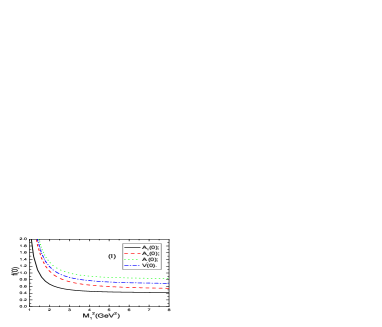
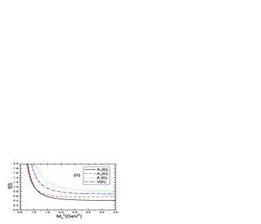
Figure 4: The weak from-factors with variations of the Borel parameters $M_{1}^{2}$ and $M_{2}^{2}$, where $M_{2}^{2}=3.0\,\rm{GeV}^{2}$ in (I) and $M_{1}^{2}=6.0\,\rm{GeV}^{2}$ in (II).

The semileptonic decays $B_{c}^{*}\to\eta_{c}\ell\nu_{\ell}$ can be described by the effective Hamiltonian ${\cal H}_{\rm eff}$,

$${\cal H}_{\rm eff} = \frac{G_{F}}{\sqrt{2}}V_{cb}\bar{c}\gamma_{\alpha}(1-\gamma_{5})b\,\bar{\nu}_{\ell}\gamma^{\alpha}(1-\gamma_{5})\ell\,,$$ (30)

where the $V_{cb}$ is the CKM matrix element and the $G_{F}$ is the Fermi constant. We take into account the effective Hamiltonian ${\cal H}_{\rm eff}$ and the weak form-factors $A_{1}(q^{2})$, $A_{+}(q^{2})$, $A_{-}(q^{2})$ and $V(q^{2})$ to obtain the squared amplitude $|T|^{2}$,

$$|T|^{2} = 4G_{F}^{2}V_{cb}^{2}(l^{\alpha}v^{\beta}+l^{\beta}v^{\alpha}-l\cdot vg^{\alpha\beta})\langle\eta_{c}(p)|j_{\alpha}(0)|B_{c}^{*}(P)\rangle\left[\langle\eta_{c}(p)|j_{\beta}(0)|B_{c}^{*}(P)\rangle\right]^{\dagger}\,,$$ (31)

where the $P$, $p$, $l$ and $v$ are the four-momenta of the $B_{c}^{*}$, $\eta_{c}$, $\ell$ and $\bar{\nu}_{\ell}$, respectively. Finally we obtain the differential decay widths,

$$d\Gamma = \sum\frac{|T|^{2}}{6m_{B_{c}^{*}}}\frac{dq^{2}}{2\pi}d\Phi(P\to q,p)\,d\Phi(q\to l,v)\,,$$ (32)

where the $d\Phi(P\to q,p)$ and $d\Phi(q\to l,v)$ are the two-body phase factors defined analogously, for example,

$$d\Phi(P\to q,p) = (2\pi)^{4}\delta^{4}(P-q-p)\frac{d^{3}\vec{p}}{(2\pi)^{3}2p_{0}}\frac{d^{3}\vec{q}}{(2\pi)^{3}2q_{0}}\,.$$ (33)

We take the revelent parameters as $G_{F}=1.166364\times 10^{-5}\,\rm{GeV}^{-2}$, $V_{cb}=40.6\times 10^{-3}$, $m_{e}=0.510998928\,\rm{MeV}$, $m_{\mu}=105.6583715\,\rm{MeV}$, $m_{\tau}=1776.82\,\rm{MeV}$ from the Particle Data Group [6], then obtain the differential decay widths and decay widths,

$$\Gamma(B_{c}^{*}\to\eta_{c}e\bar{\nu}_{e}) = 6.86^{+2.12}_{-1.83}{}^{+0.22}_{-0.21}{}^{+0.04}_{-0.04}{}^{+0.71}_{-0.65}\times 10^{-6}\,{\rm{eV}}\,,$$

$$= 6.86^{+2.25}_{-1.95}\times 10^{-6}\,{\rm{eV}}\,,$$

$$\Gamma(B_{c}^{*}\to\eta_{c}\mu\bar{\nu}_{\mu}) = 6.84^{+2.11}_{-1.82}{}^{+0.22}_{-0.22}{}^{+0.04}_{-0.04}{}^{+0.71}_{-0.65}\times 10^{-6}\,{\rm{eV}}\,,$$

$$= 6.84^{+2.24}_{-1.95}\times 10^{-6}\,{\rm{eV}}\,,$$

$$\Gamma(B_{c}^{*}\to\eta_{c}\tau\bar{\nu}_{\tau}) = 2.15^{+0.66}_{-0.57}{}^{+0.05}_{-0.05}{}^{+0.04}_{-0.03}{}^{+0.35}_{-0.30}\times 10^{-6}\,{\rm{eV}}\,,$$ (34)

$$= 2.15^{+0.75}_{-0.65}\times 10^{-6}\,{\rm{eV}}\,,$$

where the uncertainties originate from the uncertainties of the $A_{1}(q^{2})$, $A_{+}(q^{2})$, $V(q^{2})$ and $m_{B_{c}^{*}}$, sequentially. The numerical values of the differential decay widths $d\Gamma/dq^{2}$ are shown in Fig.5. The decay width of the radiative transition $B_{c}^{*}\to B_{c}\gamma$ is about tens of $\rm{eV}$ from the potential models [21], the branching fractions of the $B_{c}^{*}\to\eta_{c}\ell\bar{\nu}_{\ell}$ are of the order $10^{-7}\sim 10^{-6}$. The tiny branching fractions of the order $10^{-7}\sim 10^{-6}$ maybe escape experimental detections. The semileptonic decay widths of the $B_{c}$ mesons to charmonium states are also of the order $10^{-6}\,\rm{eV}$ [31], the corresponding branching fractions are of the order $10^{-3}$, as the $B_{c}$ mesons have much smaller width $\Gamma_{B_{c}}=1.46\times 10^{-3}\,\rm{eV}$, the semileptonic decays of the $B_{c}$ mesons to charmonium states are more easy to be observed. The $b\bar{b}$ pairs would be copiously produced at the LHCb [7], we expect that a large number of $B_{c}^{*}$ events would be accumulated, and the experimental study of the differential branching fractions of the semileptonic decays of $B^{*}_{c}$ mesons to charmonium states would be feasible. The differential branching fractions can be measured as $\Delta{\rm Br}/\Delta q^{2}$ in bins of the momentum-transfer squared $q^{2}$. The LHCb collaboration has observed the first evidence for the hadronic annihilation decay $B^{+}\to D_{s}^{+}\phi$ with significance more than $3\sigma$, the measured branching fraction is ${\rm{Br}}(B^{+}\to D_{s}^{+}\phi)=\left(1.87^{+1.25}_{-0.73}\pm 0.19\pm 0.32\right)\times 10^{-6}$ [32]. The branching fractions ${\rm{Br}}(B^{+}\to D_{s}^{+}\phi)$ and ${\rm{Br}}(B_{c}^{*}\to\eta_{c}\ell\bar{\nu}_{\ell})$ are of the same order, we still expect that the $B_{c}^{*}\to\eta_{c}\ell\bar{\nu}_{\ell}$ be observed in the future at the LHCb. On the other hand, we can take the $B_{c}^{*}\to\eta_{c}$ form-factors as basic input parameters in the phenomenological analysis of the two-body decays of the $B_{c}^{*}$ mesons, such as the $B_{c}^{*}\to\eta_{c}\pi$, $\eta_{c}\rho$, $\eta_{c}a_{0}(980)$, $\eta_{c}a_{1}(1260)$, $\eta_{c}a_{2}(1320)$, $\eta_{c}K$, $\eta_{c}K^{*}$, $\eta_{c}K_{0}(800)$, $\eta_{c}K_{1}(1270)$, $\eta_{c}K_{1}(1400)$, $\eta_{c}D$, $\eta_{c}D^{*}$, $\eta_{c}D_{0}$, $\eta_{c}D_{1}$, $\eta_{c}D_{2}$, $\eta_{c}D_{s}$, $\eta_{c}D^{*}_{s}$, $\eta_{c}D_{s0}$, $\eta_{c}D_{s1}$, $\eta_{c}D_{s2}$, etc.

$A_{1}(0)$	$A_{+}(0)$	$A_{-}(0)$	$V(0)$
$0.43\pm 0.07$	$0.57\pm 0.09$	$0.85\pm 0.15$	$0.71\pm 0.12$
$c_{1}/c_{2}$	$c_{1}/c_{2}$	$c_{1}/c_{2}$	$c_{1}/c_{2}$
$0.0484/0.0000$	$0.0710/0.0005$	$0.0719/0.0004$	$0.0715/0.0004$

Table 2: The parameters for the weak form-factors, the units of the $c_{1}$ and $c_{2}$ are $\rm{GeV}^{-2}$ and $\rm{GeV}^{-4}$, respectively.

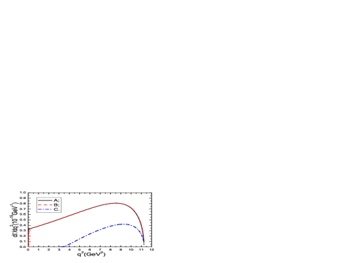
Figure 5: The differential decay widths with variations of the squared momentum $q^{2}$, the $A$, $B$ and $C$ denote $d\Gamma(B_{c}^{*}\to\eta_{c}e\bar{\nu}_{e})/dq^{2}$, $d\Gamma(B_{c}^{*}\to\eta_{c}\mu\bar{\nu}_{\mu})/dq^{2}$ and $d\Gamma(B_{c}^{*}\to\eta_{c}\tau\bar{\nu}_{\tau})/dq^{2}$, respectively.

4 Conclusion

In this article, we study the $B_{c}^{*}\to\eta_{c}$ form-factors with the three-point QCD sum rules, then take those weak form-factors as the basic input parameters to calculate the semileptonic decay widths and differential decay widths. The tiny decay widths may be observed experimentally in the future at the LHCb, while the $B_{c}^{*}\to\eta_{c}$ form-factors can be taken as basic input parameters in other phenomenological analysis.

References

• [1] S. Godfrey and N. Isgur, Phys. Rev. D32 (1985) 189; S. Godfrey, Phys. Rev. D70 (2004) 054017.
• [2] A. Abulencia et al, Phys. Rev. Lett. 97 (2006) 012002.
• [3] V. Abazov et al, Phys. Rev. Lett. 102 (2009) 092001.
• [4] T. Aaltonen et al, Phys. Rev. Lett. 100 (2008) 182002.
• [5] V. M. Abazov et al, Phys. Rev. Lett. 101 (2008) 012001.
• [6] J. Beringer et al, Phys. Rev. D86 (2012) 010001.
• [7] G. Kane and A. Pierce, ”Perspectives On LHC Physics”, World Scientific Publishing Company, Singapore, 2008.
• [8] N. Brambilla et al, arXiv:hep-ph/0412158.
• [9] M. A. Shifman, A. I. Vainshtein and V. I. Zakharov, Nucl. Phys. B147 (1979) 385, 448.
• [10] L. J. Reinders, H. Rubinstein and S. Yazaki, Phys. Rept. 127 (1985) 1.
• [11] P. Colangelo and A. Khodjamirian, arXiv:hep-ph/0010175.
• [12] S. Narison, Camb. Monogr. Part. Phys. Nucl. Phys. Cosmol. 17 (2002) 1.
• [13] P. Colangelo, G. Nardulli and N. Paver, Z. Phys. C57 (1993) 43.
• [14] E. Bagan, H. G. Dosch, P. Gosdzinsky, S. Narison and J. M. Richard, Z. Phys. C64 (1994) 57.
• [15] V. V. Kiselev, A. K. Likhoded and A. I. Onishchenko, Nucl. Phys. B569 (2000) 473.
• [16] S. S. Gershtein, V. V. Kiselev, A. K. Likhoded and A. V. Tkabladze, Phys. Usp. 38 (1995) 1; V. V. Kiselev, A. E. Kovalsky and A. K. Likhoded, Nucl. Phys. B585 (2000) 353; V. V. Kiselev, arXiv:hep-ph/0211021; K. Azizi, R. Khosravi and V. Bashiry, Eur. Phys. J. C56 (2008) 357; K. Azizi, F. Falahati, V. Bashiry and S. M. Zebarjad, Phys. Rev. D77 (2008) 114024; K. Azizi and R. Khosravi, Phys. Rev. D78 (2008) 036005; N. Ghahramany, R. Khosravi and K. Azizi, Phys. Rev. D78 (2008) 116009.
• [17] M. Neubert, Phys. Rept. 245 (1994) 259.
• [18] B .L. Ioffe and A. V. Smilga, Nucl. Phys. B216 (1983) 373.
• [19] D. S. Du, J. W. Li and M. Z. Yang, Eur. Phys. J. C37 (2004) 173.
• [20] Z. G. Wang, arXiv:1203.6252.
• [21] D. Ebert, R. N. Faustov and V. O. Galkin, Phys. Rev. D67 (2003) 014027; and references therein.
• [22] S. N. Gupta and J. M. Johnson, Phys. Rev. D53 (1996) 312.
• [23] J. Zeng, J. W. Van Orden and W. Roberts, Phys. Rev. D52 (1995) 5229.
• [24] L. P. Fulcher, Phys. Rev. D60 (1999) 074006.
• [25] S. S. Gershtein, V. V. Kiselev, A. K. Likhoded and A. V. Tkabladze, Phys. Rev. D51 (1995) 3613.
• [26] E. J. Eichten and C. Quigg, Phys. Rev. D49 (1994) 5845.
• [27] C. T. H. Davies et al, Phys. Lett. B382 (1996) 131.
• [28] V. A. Novikov, L. B. Okun, M. A. Shifman, A. I. Vainshtein, M. B. Voloshin and V. I. Zakharov, Phys. Rept. 41 (1978) 1; N. G. Deshpande and J. Trampetic, Phys. Lett. B339 (1994) 270.
• [29] S. S. Gershtein, M. Yu. Khlopov, JETP Lett. 23 (1976) 338; M. Yu. Khlopov, Sov. J. Nucl. Phys. 28 (1978) 583.
• [30] S. Narison, Phys. Lett. B693 (2010) 559; S. Narison, Phys. Lett. B706 (2012) 412; S. Narison, Phys. Lett. B707 (2012) 259.
• [31] D. Ebert, R. N. Faustov and V. O. Galkin, Phys. Rev. D82 (2010) 034019; Z. H. Wang, G. L. Wang and C. H. Chang, J. Phys. G39 (2012) 015009; W. F. Wang, Y. Y. Fan and Z. J. Xiao, arXiv:1212.5903; C. F. Qiao and R. L. Zhu, Phys. Rev. D87 (2013) 014009.
• [32] R. Aaij et al, JHEP 1302 (2013) 043.