Anomalous Shock Displacement Probabilities for a Perturbed Scalar Conservation Law

Abstract

We consider an one-dimensional conservation law with random space-time forcing and calculate using large deviations the exponentially small probabilities of anomalous shock profile displacements. Under suitable hypotheses on the spatial support and structure of random forces, we analyze the scaling behavior of the rate function, which is the exponential decay rate of the displacement probabilities. For small displacements we show that the rate function is bounded above and below by the square of the displacement divided by time. For large displacements the corresponding bounds for the rate function are proportional to the displacement. We calculate numerically the rate function under different conditions and show that the theoretical analysis of scaling behavior is confirmed. We also apply a large-deviation-based importance sampling Monte Carlo strategy to estimate the displacement probabilities. We use a biased distribution centered on the forcing that gives the most probable transition path for the anomalous shock profile, which is the minimizer of the rate function. The numerical simulations indicate that this strategy is much more effective and robust than basic Monte Carlo.

1 Introduction

It is well known that nonlinear waves are not very sensitive to perturbations in initial conditions or ambient medium inhomogeneities. This is in contrast to linear waves in random media where even weak inhomogeneities can affect significantly wave propagation over long times and distances. It is natural, therefore to consider perturbations of shock profiles of randomly forced conservation laws as rare events and use large deviations theory. The purpose of this paper is to calculate probabilities of anomalous shock profile displacements for randomly perturbed one-dimensional conservation laws. We analyze the rate function that characterizes the exponential decay of displacement probabilities and show that under suitable hypotheses on the random forcing they have scaling behavior relative to the size of the displacement and the time interval on which it occurs.

The theory of large deviations for conservation laws with random forcing is an extension of the Freidlin-Wentzell theory of large deviations [10, 7] to partial differential equations. This has been carried out extensively [1, 2, 18] and we use this theory here. We are interested in a more detailed analysis of the exponential probabilities of anomalous shock profile displacements, which leads to an analysis of the rate function associated with large deviations for this particular class of rare events. We derive upper and lower bounds for the exponential decay rate of the small probabilities using suitable test functions for the variational problem involving the rate function. This is the main result of this paper. The applications we have in mind come from uncertainty quantification [13] in connection with simplified models of flow and combustion in a scramjet. Numerical calculations of the exponential decay rates from variational principles associated with the rate function have been carried out before [9, 26]. We carry out such numerical calculations here and confirm the scaling behavior of bounds obtained theoretically. We use a gradient descent method to do the optimization numerically and we note that its convergence is quite robust even though the functional under consideration is not known to be convex. This robustness suggests the Monte Carlo simulations with importance sampling using a change of measure based on the minimizer of the discrete rate function is likely to effective. Our simulations show that indeed such importance sampling Monte Carlo performs much better than the basic Monte Carlo method.

The paper is organized as follows. In Section 2 we formulate the one-dimensional conservation law problem. In Section 3 we state the large deviation principle and identify the rate function which we will use. In Section 4 we give a simple, explicitly computable case of shock profile displacement probabilities that can be used to compare with the results of the large deviation theory. Section 5 contains the main results of the paper, which as the upper and lower bounds for the exponential decay rate of the displacement probabilities, under different conditions on the random forcing. We identify scaling behavior of these probabilities, relative to size of the displacement and the time interval of interest. In Section 6 we introduce a discrete form for the conservation law and the associated large deviations, and calculate numerically the displacement probabilities from the discrete variational principle. In Section 7 we implement importance sampling Monte Carlo based on the minimizer of the discrete rate function and we compare it with the basic Monte Carlo method. We end with a brief section summarizing the paper and our conclusions.

2 The perturbed conservation law

We consider the scalar viscous conservation law:

$$u_{t}+(F(u))_{x}=(Du_{x})_{x},\quad\quad x\in\mathbb{R},\quad t\in[0,\infty),$$ (1)

$$u(t=0,x)=u_{0}(x),\quad\quad x\in\mathbb{R}.$$ (2)

Here $F\in{\cal C}^{2}(\mathbb{R})$ and the initial condition satisfies $u_{0}(x)\to{u}_{\pm}$ as $x\to\pm\infty$ where ${u}_{-}<{u}_{+}$. We are interested in traveling wave solutions of the form ${U}(x-\gamma t)$, where the ${\cal C}^{2}$ profile ${U}$ satisfies ${U}(x)\to{u}_{\pm}$ as $x\to\pm\infty$ and the wave speed $\gamma$ is given by the Rankine-Hugoniot condition

$$\gamma=\frac{F({u}_{+})-F({u}_{-})}{{u}_{+}-{u}_{-}}.$$ (3)

A traveling wave ${U}$ with wave speed $\gamma$ exists provided the following conditions are fulfilled:

$$F(u)-F({u}_{-})>\gamma(u-{u}_{-}),\quad\forall u\in(u_{+},u_{-}),$$ (4)

$$F^{\prime}({u}_{+})<\gamma<F^{\prime}({u}_{-}).$$ (5)

The first condition is the Oleinik entropy condition [14] and the second one is the Lax entropy condition [16]. Under these conditions the traveling wave profile exists, it is the solution of the ordinary differential equation

$$U_{x}=\frac{1}{D}\big{(}F(U)-F(u_{-})-\gamma(U-u_{-})\big{)},\quad\quad U(x)\stackrel{{\scriptstyle x\to-\infty}}{{\longrightarrow}}u_{-},$$

and it is orbitally stable, which means that perturbations of the profile decay in time, and thus initial conditions near the traveling wave profile converge to it. Note that a physically admissible viscous profile must have the stability property; otherwise, it would not be observable. As noted in [15], the motivating idea behind the orbital stability result is that in the stabilizing process, information is transferred from spatial decay of the profile ${U}$ at infinity to temporal decay of the perturbation.

The purpose of this paper is to address another type of stability, that is, the stability with respect to external noise. We consider the perturbed scalar viscous conservation law with additive noise:

$$u^{\varepsilon}_{t}+(F(u^{\varepsilon}))_{x}=(Du^{\varepsilon}_{x})_{x}+\varepsilon\dot{W}(t,x),\quad\quad x\in\mathbb{R},\quad t\in[0,\infty),$$ (6)

$$u^{\varepsilon}(t=0,x)={U}(x),\quad\quad x\in\mathbb{R}.$$ (7)

Here $\varepsilon$ is a small parameter, $W(t,x)$ is a zero-mean random process (described below), and the dot stands for the time derivative. We would like to address the stability of the traveling wave ${U}(x-\gamma t)$ driven by the noise $\varepsilon\dot{W}$. Motivated by an application modeling combustion in a scramjet [13, 25], we have in mind a specific rare event, which is an exceptional or anomalous shift of the position of the traveling wave compared to the unperturbed motion with the constant velocity $\gamma$.

We consider mild solutions which satisfy (denoting $u^{\varepsilon}(t)=(u^{\varepsilon}(t,x))_{x\in\mathbb{R}}$)

$$u^{\varepsilon}(t)=S(t)U-\int_{0}^{t}S(t-s)N(u^{\varepsilon}(s))ds+\varepsilon\int_{0}^{t}S(t-s){dW}(s),$$ (8)

where $S(t)$ is the heat semi-group with kernel

$$S(t,x,y)=\frac{1}{\sqrt{2\pi Dt}}\exp\Big{(}-\frac{(x-y)^{2}}{2Dt}\Big{)},$$

and $N(u)(x)=(F(u(x)))_{x}$. The main result about the heat kernel [5, Chap. XVI, Sec. 3] is as follows.

Lemma 1.

If $f=(f(t))_{t\in[0,T]}\in L^{2}([0,T],H^{-1}(\mathbb{R}))$, then the function $\int_{0}^{t}S(t-s)f(s)ds$ is in $L^{2}([0,T],H^{1}(\mathbb{R}))\cap{\cal C}([0,T],L^{2}(\mathbb{R}))$.

A white noise or cylindrical Wiener process $B(t,x)$ in the Hilbert space $L^{2}(\mathbb{R})$ is such that for any complete orthonormal system $(f_{n}(x))_{n\geq 1}$ of $L^{2}(\mathbb{R})$, there exists a sequence of independent Brownian motions $(\beta_{n}(t))_{n\geq 1}$ such that

$$B(t,x)=\sum_{n=1}^{\infty}\beta_{n}(t)f_{n}(x).$$ (9)

$B(t,x)$ can be seen as the (formal) spatial derivative of the Brownian sheet on $[0,\infty)\times\mathbb{R}$, which means that it is the Gaussian process with mean zero and covariance $\mathbb{E}[B(t,x)B(s,y)]=s\wedge t\,\delta(x-y)$. Note that the sum (9) does not converge in $L^{2}$ but in any Hilbert space $H$ such that the embedding from $L^{2}(\mathbb{R})$ to $H$ is Hilbert-Schmidt. Therefore, the image of the process $B$ by a linear mapping on $L^{2}(\mathbb{R})$ is a well-defined process in the Sobolev space $H^{k}(\mathbb{R})$ (for $k=0$, we take the convention $H^{0}=L^{2}$) when the mapping is Hilbert-Schmidt from $L^{2}(\mathbb{R})$ into $H^{k}(\mathbb{R})$. Then, if the kernel $\Phi$ is Hilbert-Schmidt in the sense that

$$\sum_{n=1}^{\infty}\|\Phi f_{n}\|_{H^{k}(\mathbb{R})}^{2}=\sum_{j=0}^{k}\|\partial_{x}^{j}\Phi(\cdot,\cdot)\|_{L^{2}(\mathbb{R}\times\mathbb{R})}^{2}<\infty,$$

then the random process $W=\Phi B$,

$$W(t,x)=\int\Phi(x,x^{\prime})B(t,x^{\prime})dx^{\prime}$$

is well-defined in $H^{k}(\mathbb{R})$. It is a zero-mean Gaussian process with covariance function given by

$$\mathbb{E}[W(t,x)W(t^{\prime},x^{\prime})]=t\wedge t^{\prime}\,C(x,x^{\prime}),$$

$$C(x,x^{\prime})=\Phi\Phi^{T}(x,x^{\prime})=\int\Phi(x,x^{\prime\prime})\Phi(x^{\prime},x^{\prime\prime})dx^{\prime\prime},$$

where $\Phi^{T}$ stands for the adjoint of $\Phi$.

As an example, we may think at $\Phi(x,x^{\prime})=\Phi_{0}(x)\Phi_{1}(x-x^{\prime})$ with $\Phi_{0}\in H^{k}(\mathbb{R})$ and $\Phi_{1}\in H^{k}(\mathbb{R})$. In this case $\Phi_{0}$ characterizes the spatial support of the additive noise and $\Phi_{1}$ characterizes its local correlation function. In the limit $\Phi_{0}(x)=1$ and $\Phi_{1}(x-x^{\prime})=\delta(x-x^{\prime})$, the process $\dot{W}(t,x)$ in (6) is a space-time white noise.

By adapting the technique used in [5, Chap. XVI, Sec. 3] we obtain the following lemma.

Lemma 2.

If $\Phi$ is Hilbert-Schmidt from $L^{2}$ into $L^{2}$, then $Z(t)=\int_{0}^{t}S(t-s){dW}(s)$ belongs to $L^{2}([0,T],H^{1}(\mathbb{R}))\cap{\cal C}([0,T],L^{2}(\mathbb{R}))$ almost surely. If $\Phi$ is Hilbert-Schmidt from $L^{2}$ into $H^{1}$, then $Z(t)$ belongs to $L^{2}([0,T],H^{2}(\mathbb{R}))\cap{\cal C}([0,T],H^{1}(\mathbb{R}))$ almost surely.

Proof.

See Appendix A. ∎

3 Large deviation principle

In this section we state a large deviation principle (LDP) for the solution $(u^{\varepsilon}(t,x))_{t\in[0,T],x\in\mathbb{R}}$ of the randomly perturbed scalar conservation law (6). It generalizes the classical Freidlin-Wentzell principle for finite-dimensional diffusions. Throughout this paper, we assume that the flux $F$ is a $\mathcal{C}^{2}$ function with bounded first and second derivatives.

Assumption 3.

In this paper, the flux $F$ is a $\mathcal{C}^{2}$ function and there exists $C_{F}<\infty$ such that $\|F^{\prime}\|_{L^{\infty}(\mathbb{R})}$ and $\|F^{\prime\prime}\|_{L^{\infty}(\mathbb{R})}$ are bounded by $C_{F}$.

Remark. Assumption 3 is merely a technical assumption to simplify the proofs of Proposition 4 and 5 and obviously it violates the convexity of fluxes in conservation laws. From the physical point of view, for a general flux $F$, we can choose a very large constant $M$ and let $F_{M}(u)=F(u)$ for $|u|\leq M$ and saturate $F_{M}(u)$ for $|u|>M$. If $[-M,M]$ can cover the range of interest of $u$, then $F_{M}(u)=F(u)$. Without a proof, we point out that this physical argument can be proven mathematically: if $u^{\varepsilon}_{t}$, $u^{\varepsilon}_{x}$ and $u^{\varepsilon}_{xx}$ in (6) are continuous on $[0,T]\times\mathbb{R}$ and $\dot{W}$ is bounded on $[0,T]\times\mathbb{R}$, then the parabolic maximum principle implies that $|u^{\varepsilon}|$ is bounded on $[0,T]\times\mathbb{R}$ and thus we can find $M<\infty$. The technical difficulty is that $W$ is not differentiable in time so we can not apply the parabolic maximum principle directly. However, we can consider a modified $\tilde{u}^{\varepsilon}$ by replacing $W$ by a smooth $\tilde{W}$ in (6) and show that $\|\tilde{u}^{\varepsilon}(t)\|_{L^{\infty}(\mathbb{R})}\to\|u^{\varepsilon}(t)\|_{L^{\infty}(\mathbb{R})}$ as $\tilde{W}\to W$.

We first describe the functional space to which the solution of the perturbed conservation law belongs.

Proposition 4.

If $\Phi$ is Hilbert-Schmidt from $L^{2}$ to $H^{1}$, then for any $\varepsilon>0$ there is a unique solution $u^{\varepsilon}$ to (8) in the space ${\cal E}^{1}$ almost surely, where

$${\cal E}^{1}=\big{\{}(u(t,x))_{t\in[0,T],x\in\mathbb{R}}:~{}(u(t,x)-U(x))_{t\in[0,T],x\in\mathbb{R}}\in{\cal C}([0,T],H^{1}(\mathbb{R}))\big{\}}.$$

Proof.

See Appendix B.1 ∎

The rate function of the LDP is defined in terms of the mild solution of the control problem

$$u_{t}+(F(u))_{x}=(Du_{x})_{x}+\Phi h(t,x),\quad\quad x\in\mathbb{R},\quad t\in[0,T],$$ (11)

$$u(t=0,x)={U}(x),\quad\quad x\in\mathbb{R},$$

where $h\in L^{2}([0,T],L^{2}(\mathbb{R}))$. The solution $u$ to this problem is denoted by ${\cal H}[h]$ and ${\cal H}$ is a mapping from $L^{2}([0,T],L^{2}(\mathbb{R}))$ to ${\cal E}^{1}$ provided $\Phi$ is Hilbert-Schmidt from $L^{2}$ to $H^{1}$. The following proposition is an extension of the LDP proved in [1].

Proposition 5.

If $\Phi$ is Hilbert-Schmidt from $L^{2}$ to $H^{1}$, then the solutions $u^{\varepsilon}$ satisfy a large deviation principle in ${\cal E}^{1}$ with the good rate function

$$I(u)=\inf_{h,u={\cal H}[h]}\frac{1}{2}\int_{0}^{T}\|h(t,\cdot)\|_{L^{2}}^{2}dt,$$ (12)

with the convention $\inf\emptyset=\infty$.

Proof.

See Appendix B.2. ∎

In fact, $I(u)<\infty$ if and only if $u$ is in the range of ${\cal H}$. The LDP means that, for any $A\subset{\cal E}^{1}$, we have

$$-{\cal J}(\mathring{A})\leq\liminf_{\varepsilon\to 0}\varepsilon^{2}\log\mathbb{P}(u^{\varepsilon}\in A)\leq\limsup_{\varepsilon\to 0}\varepsilon^{2}\log\mathbb{P}(u^{\varepsilon}\in A)\leq-{\cal J}(\overline{A}),$$ (13)

with

$${\cal J}(A)=\inf_{u\in A}I(u).$$ (14)

Note that the interior $\mathring{A}$ and closure $\overline{A}$ are taken in the topology associated with ${\cal E}^{1}$.

Although the convexity of the rate function $I$ is unknown, it is possible to show that $I$ satisfies the maximum principle: if the set of the rare event $A$ does not contain the exact solution $U(x-\gamma t)$, then $\inf_{u\in A}I(u)$ attains its minimum at the boundary of $A$.

Proposition 6.

If $U(x-\gamma t)\notin A$ and $u\in\mathring{A}$, then there exists a sequence $\{u^{n}\}$ in $\mathcal{E}^{1}$ such that $I(u^{n})<I(u)$ and $u^{n}\to u$ in $\mathcal{E}^{1}$ as $n\to\infty$. As a consequence, any $u\in\mathring{A}$ can not be a local minimizer of $I$.

Proof.

See Appendix B.3. ∎

4 Wave displacement from an elementary point of view

In this paper we are interested in estimating the probability of large deviations from the deterministic path ${U}(x-\gamma t)$. In this section, we first study in a very elementary way how the center of the solution $u^{\varepsilon}$ at time $T$ can deviate from its unperturbed value. The center of a function $u\in{\mathcal{E}}^{1}$ is defined as

$${\cal C}[u](t)=-\frac{\int_{-\infty}^{\infty}[u(t,x)-U(x)]dx}{u_{-}-u_{+}},$$ (15)

provided that the integral is well-defined.

Proposition 7.

If the covariance function $C$ is in $L^{1}(\mathbb{R}\times\mathbb{R})$, then the center of $u^{\varepsilon}$ is well-defined for any time $t\in[0,T]$ almost surely and it is given by

$${\cal C}[u^{\varepsilon}](t)=\gamma t-\varepsilon\frac{\int W(t,x)dx}{u_{-}-u_{+}}.$$ (16)

It is a Gaussian process with mean $\gamma t$ and covariance

$$\mathbf{Cov}\big{(}{\cal C}[u^{\varepsilon}](t),{\cal C}[u^{\varepsilon}](t^{\prime})\big{)}=\varepsilon^{2}\frac{\iint C(x,x^{\prime})dxdx^{\prime}}{(u_{-}-u_{+})^{2}}\,t\wedge t^{\prime}.$$ (17)

Proof.

See Appendix C. ∎

In the absence of noise, the center of the solution increases linearly as $\gamma t$. In the presence of noise we can characterize the probability of the rare event

$$B=\big{\{}u\in{\cal E}^{1},\,{\cal C}[u](T)\geq\gamma T+x_{0}\big{\}},$$ (18)

where $x_{0}\in[0,\infty)$.

Proposition 8.

If the covariance function $C$ is in $L^{1}(\mathbb{R}\times\mathbb{R})$, then

$$\mathbb{P}(u^{\varepsilon}\in B)\sim\exp\Big{(}-\frac{x_{0}^{2}(u_{-}-u_{+})^{2}}{2\varepsilon^{2}T\iint C(x,x^{\prime})dxdx^{\prime}}\Big{)}.$$ (19)

The approximate equality means that

$$\lim_{\varepsilon\to 0}\varepsilon^{2}\log\mathbb{P}(u^{\varepsilon}\in B)=-\frac{x_{0}^{2}(u_{-}-u_{+})^{2}}{2T\iint C(x,x^{\prime})dxdx^{\prime}}.$$

This proposition is a direct corollary of Proposition 7.

If $x_{0}=0$ then $U(x-\gamma t)\in B$ and $\mathbb{P}(u^{\varepsilon}\in B)=1/2$. If $x_{0}>0$ then the set $B$ is indeed exceptional in that it corresponds to the event in which the center of the profile is anomalously ahead of its expected position. Note that the scaling $x_{0}^{2}/T$ in (19) corresponds to that of the exit problem of a Brownian particle.

The LDP for $u^{\varepsilon}$ stated in Proposition 5 is not used here for two reasons:

1. It does not give a good result because the interior of $B$ in ${\mathcal{E}}^{1}$ is empty (since we can construct a sequence of functions bounded in $H^{1}$ that blows up in $L^{1}$).

2. The distribution of the center ${\cal C}[u^{\varepsilon}](T)$ is here explicitly known for any $\varepsilon$. This is fortunate and it is not always true. When the rare event is more complex, than the LDP for $u^{\varepsilon}$ is useful as we will show in the next section.

5 Wave displacement from the large deviations point of view

5.1 The framework and result

In this section, we use the large deviation principle to compute the probability of the rare event that the perturbed traveling wave is the same profile but with the displacement $x_{0}$ at time $T$:

$$A=\{u\in\mathcal{E}^{1}\mbox{ such that }u(0,x)=U(x),\,u(T,x)=U(x-\gamma T-x_{0})\}.$$ (20)

The value of the rate function heavily depends on the kernel $\Phi$ and formally the simplest kernel we can have is the identity operator. Of course, the identity operator is not Hilbert-Schmidt, but with the given $A$, we can construct a Hilbert-Schmidt $\Phi$ such that $\Phi$ is approximately the identity in the region of interest.

Assumption 9.

1. We assume that the center of transition of $U(x)$ in (20) is $0$ and $x_{0}+\gamma T\geq 0$.

2. The kernel $\Phi^{l_{c}}_{L_{0}}$ has the following form:

   $$\Phi^{l_{c}}_{L_{0}}(x,x^{\prime})=\sigma\phi_{0}\Big{(}\frac{x}{L_{0}}\Big{)}\frac{1}{l_{c}}\phi_{1}\Big{(}\frac{x-x^{\prime}}{l_{c}}\Big{)},$$ (21)

   where $\sigma$, $L_{0}$ and $l_{c}$ are positive constants.

3. $\phi_{0}$ and $\phi_{1}$ are $L^{1}\cap H^{1}$ functions so that their Fourier transforms are well-defined in $\mathbb{R}$ and $\Phi$ is Hilbert-Schmidt from $L^{2}$ to $H^{1}$ (see Lemma 12). $\phi_{0}$ and $\phi_{1}$ are normalized so that $\phi_{0}(0)=\hat{\phi}_{1}(0)=1$.

4. $\phi_{0}\in\mathcal{C}^{\infty}$ is positive valued and $\hat{\phi}_{1}$ is nonzero. In addition, $1/\phi_{0}(x)$ and $1/\hat{\phi}_{1}(\xi)$ have at most polynomial growth at $\pm\infty$.

5. $\phi_{0}(x)$ is increasing on $x\in(-\infty,-1)$, decreasing on $x\in(1,\infty)$ and identically equal to $1$ on $x\in[-1,1]$. By this setting, the support of the noise kernel $\Phi$ is roughly $[-L_{0},L_{0}]$.

The following theorem is the main result of this section, and the proof will be given in the next two subsections.

Theorem 10.

Let $A$ be defined by (20). There exists a constant $C_{0}$ such that for all $\Phi^{l_{c}}_{L_{0}}$ satisfying Assumption 9 with $L_{0}=\gamma T+x_{0}+C_{0}$, the quantity $\mathcal{J}(A)$ of the large deviation problem (11) generated by $\Phi^{l_{c}}_{L_{0}}$ has the following asymptotic (in the sense that $l_{c}\to 0$) scales:

$$\mathcal{J}(A)=\inf_{u\in A}I(u)\overset{l_{c}\to 0}{=}\begin{cases}\Theta(x_{0}^{2}),\quad&\text{for $|x_{0}|$ small and any fixed $T$,}\\ \Theta(x_{0}^{2}/T),\quad&\text{for $|x_{0}|$ small and $T$ small,}\\ \Theta(|x_{0}|),\quad&\text{for $|x_{0}|$ large and any fixed $T$,}\\ \Theta(|x_{0}|/T),\quad&\text{for $|x_{0}|$ large and $T$ small,}\\ \Theta(1/T),\quad&\text{for $T$ small and any fixed $x_{0}$.}\end{cases}$$ (22)

Here $\mathcal{J}(A)\overset{l_{c}\to 0}{=}\Theta(x_{0}^{2})$ and similar expressions mean that there are constants $C_{1}$ and $C_{2}$ with the units such that $C_{1}x_{0}^{2}$ and $C_{2}x_{0}^{2}$ are dimensionless and $C_{1}x_{0}^{2}\leq\mathcal{J}(A)\leq C_{2}x_{0}^{2}$ as $l_{c}\to 0$.

Proof.

See Section 5.2 and 5.3. ∎

Remark. $C_{0}=\max\{C_{v},C_{w}\}$, where $C_{v}$ and $C_{w}$ will be determined in Lemma 14 and 18, respectively. $L_{0}=\gamma T+x_{0}+C_{0}$ means that the range of noise covers the region of interest of $A$ so that the rare event $A$ is possible and at the same time the range is not too large to cause the waste of energy; the small $l_{c}$ means that the noise in this region is weakly correlated and can be treated as the white noise.

We note that there are two occurrences of $T$ in $\mathcal{J}(A)$: in (12), we integrate the $\|h(t,\cdot)\|_{L^{2}}^{2}$ from $0$ to $T$, and the rare event $A$ is $T$-dependent. These two occurrences of $T$ would make the $T$-dependence of $\mathcal{J}(A)$ nontrivial; if $T$ is small, the $T$-dependence in (20) is negligible and we can have the scale in $T$. Therefore, if the traveling wave is stationary ($\gamma=0$), then $A$ has no $T$-dependence so the sharper bounds can be obtained.

Corollary 11.

If $\gamma=0$, then (22) can be refined:

$$\mathcal{J}(A)=\inf_{u\in A}I(u)\overset{l_{c}\to 0}{=}\begin{cases}\Theta(x_{0}^{2}/T),\quad&\text{for $|x_{0}|$ small,}\\ \Theta(|x_{0}|),\quad&\text{for $|x_{0}|$ large and any fixed $T$,}\\ \Theta(|x_{0}|/T),\quad&\text{for $|x_{0}|$ large and $T$ small,}\\ \Theta(1/T),\quad&\text{for any fixed $x_{0}$.}\end{cases}$$ (23)

Proof.

See Section 5.2 and 5.3. ∎

Remark. The case that both $|x_{0}|$ and $T$ are large is not clear even if $\gamma=0$. This is because $\mathcal{J}(A)=\Theta(|x_{0}|/T)$ for $|x_{0}|\gg T$, and $\mathcal{J}(A)=\Theta(x_{0}^{2}/T)$ for $|x_{0}|\ll T$; when both $x_{0}$ and $T$ are large, $\mathcal{J}(A)$ is the mixture of $\Theta(|x_{0}|/T)$ and $\Theta(x_{0}^{2}/T)$ so it is difficult to estimate the bounds.

In the rest of this subsection we discuss two relevant issues about this framework. We first show that the given kernel $\Phi^{l_{c}}_{L_{0}}$ in Assumption 9 is indeed Hilbert-Schmidt from $L^{2}$ to $H^{1}$.

Lemma 12.

If $\phi_{0}$ and $\phi_{1}$ are both in $L^{1}\cap H^{k}$ for $k\geq 1$, then the kernel $\Phi^{l_{c}}_{L_{0}}$ of the form (21) is Hilbert-Schmidt from $L^{2}$ to $H^{k}$.

Proof.

See Appendix D.1. ∎

The other issue is that $A$ has no interior and therefore $\mathcal{J}(\mathring{A})=\infty$, which gives a trivial lower bound in the large deviation framework; to avoid this triviality, a rigorous way is to consider instead the (closed) rare event $A_{\delta}$ with a small $\delta>0$:

$$A_{\delta}=\{u\in\mathcal{E}^{1}\mbox{ such that }u(0,\cdot)=U,\,\|u(T,\cdot)-U(\cdot-\gamma T-x_{0})\|_{H^{1}}\leq\delta\}.$$ (24)

By Proposition 5, we have

$$-\mathcal{J}(\mathring{A_{\delta}})\leq\liminf_{\varepsilon\to 0}\varepsilon^{2}\log\mathbb{P}(u^{\varepsilon}\in A_{\delta})\leq\limsup_{\varepsilon\to 0}\varepsilon^{2}\log\mathbb{P}(u^{\varepsilon}\in A_{\delta})\leq-\mathcal{J}(A_{\delta}).$$ (25)

In addition, the following lemma shows that $\mathcal{J}(A_{\delta})$ converges to $\mathcal{J}(A)$ as $\delta\to 0$.

Lemma 13.

By definition $\mathcal{J}(A_{\delta})$ is a decreasing function with $\delta$ and bounded from above by $\mathcal{J}(A)$. In addition,

$$\lim_{\delta\to 0}\mathcal{J}(A_{\delta})=\mathcal{J}(A).$$

Proof.

See Appendix D.2. ∎

By Lemma 13 and the fact that $\mathcal{J}(\mathring{A_{\delta}})\leq\mathcal{J}(A)$,

$$-\mathcal{J}(A)\leq-\mathcal{J}(\mathring{A_{\delta}}) \leq\liminf_{\varepsilon\to 0}\varepsilon^{2}\log\mathbb{P}(u^{\varepsilon}\in A_{\delta})$$

$$\leq\limsup_{\varepsilon\to 0}\varepsilon^{2}\log\mathbb{P}(u^{\varepsilon}\in A_{\delta})\leq-\mathcal{J}(A_{\delta})\overset{\delta\to 0}{\to}-\mathcal{J}(A).$$

Namely, for $\varepsilon$ and $\delta$ small, we have

$$\mathbb{P}(u^{\varepsilon}\in A_{\delta})\sim\exp\left(-\frac{1}{\varepsilon^{2}}\mathcal{J}(A)\right),$$

and it thus suffices to consider the bounds for $\mathcal{J}(A)$.

Remark. We can compare the results stated in Theorem 10, valid under Assumption 9, and the ones stated in Proposition 19. First we can check that $A\subset B$. Second we can anticipate that in fact $B$ is not much larger than $A$ because it seems reasonable that the most likely paths that achieve ${\mathcal{C}}[u](T)\geq\gamma T+x_{0}$ should be of the stable form $U(x-\gamma T-x_{0})$ at time $t=T$. This conjecture can indeed be verified as we now show. Note that

$$\iint C(x,x^{\prime})dxdx^{\prime}=\int\Big{[}\int\Phi(x,x^{\prime})dx\Big{]}^{2}dx^{\prime}.$$

If the kernel $\Phi^{l_{c}}_{L_{0}}$ is of the form (21), then we find

$$\iint C(x,x^{\prime})dxdx^{\prime}=\frac{\sigma^{2}L_{0}}{2\pi}\int|\hat{\phi}_{1}(\frac{l_{c}}{L_{0}}\xi)|^{2}|\hat{\phi}_{0}(\xi)|^{2}d\xi.$$

By assuming $l_{c}\ll L_{0}$ (and $\hat{\phi}_{1}(0)=1$) as in Assumption 9, then this simplifies to

$$\iint C(x,x^{\prime})dxdx^{\prime}\simeq\sigma^{2}L_{0}\int\phi_{0}(x)^{2}dx.$$

Therefore, from Theorem 10 (in which $L_{0}=\gamma T+x_{0}+C_{0}$), we get

$$\iint C(x,x^{\prime})dxdx^{\prime}=\begin{cases}\Theta(x_{0}),\quad&\text{for $x_{0}$ large and $T$ small or fixed,}\\ \Theta(1),\quad&\text{for $x_{0}$ and $T$ small or fixed,}\end{cases}$$

which gives with (19)

$$\mathbb{P}(u^{\varepsilon}\in B)\sim\exp\left(-\frac{1}{\varepsilon^{2}}{\mathcal{J}}(B)\right)$$

with

$${\mathcal{J}}(B)=\begin{cases}\Theta(x_{0}^{2}),\quad&\text{for $|x_{0}|$ small and any fixed $T$,}\\ \Theta(x_{0}^{2}/T),\quad&\text{for $|x_{0}|$ small and $T$ small,}\\ \Theta(|x_{0}|),\quad&\text{for $|x_{0}|$ large and any fixed $T$,}\\ \Theta(|x_{0}|/T),\quad&\text{for $|x_{0}|$ large and $T$ small,}\\ \Theta(1/T),\quad&\text{for $T$ small and any fixed $x_{0}$,}\end{cases}$$

as in (22). We therefore recover the same asymptotic scales as in Theorem 10.

5.2 Proof of Theorem 10 for small $|x_{0}|$

Here we prove the bounds for $\mathcal{J}(A)$ in (22) and (23) when $|x_{0}|$ is small and the bound $\Theta(1/T)$ for fixed $x_{0}$. We first consider the upper bounds. By definition, $\mathcal{J}(A)\leq I(u)$ for any $u\in A$; therefore the idea to obtain the upper bound is to find good test functions $u$.

For $|x_{0}|$ small, we use the linear shifted profile as the test function:

$$v(t,x)=U(x-(t/T)(\gamma T+x_{0})).$$

If the kernel $\Phi^{l_{c}}_{L_{0}}\approx\sigma^{-2}$ in the region of interest, then

$$\mathcal{J}(A)=\inf_{u\in A}I(u)\leq I(v)\lesssim\frac{1}{2\sigma^{2}}\int_{0}^{T}\|v_{t}+F(v)_{x}-Dv_{xx}\|_{L^{2}}^{2}dt.$$ (26)

We show (26) rigorously by the following lemmas:

Lemma 14.

Given the traveling wave $U(x)$ in (20), there exists $C_{v}\geq 1$ such that, uniformly in $x_{0}$ and $T$ and for all $t\in[0,T]$,

$$\|[\phi_{0}^{-1}(\cdot/L_{0})-1]U_{x}(\cdot-(t/T)(\gamma T+x_{0}))\|_{L^{2}}^{2}\leq 1.$$ (27)

where $L_{0}=\gamma T+x_{0}+C_{v}$.

Proof.

See Appendix D.3. ∎

Lemma 15.

Let $v(t,x)=U(x-(t/T)(\gamma T+x_{0}))$. Given $L_{0}=x_{0}+\gamma T+C_{v}$ in Lemma 14, $\Phi^{l_{c}}_{L_{0}}$ satisfying Assumption 9, and $h^{l_{c}}_{L_{0}}$ defined by

$$v_{t}+F(v)_{x}-Dv_{xx}=\Phi^{l_{c}}_{L_{0}}h^{l_{c}}_{L_{0}},$$ (28)

then

$$\int_{0}^{T}\|h^{l_{c}}_{L_{0}}(t,\cdot)\|_{L^{2}}^{2}dt\overset{l_{c}\to 0}{\to}\frac{1}{\sigma^{2}}\int_{0}^{T}\|(v_{t}+F(v)_{x}-Dv_{xx})/\phi_{0}(\cdot/L_{0})\|_{L^{2}}^{2}dt.$$ (29)

Proof.

See Appendix D.4. ∎

Now we are ready to prove (26). By Lemma 15, we have

$$I(v)\leq\frac{1}{2}\int_{0}^{T}\|h^{l_{c}}_{L_{0}}(t,\cdot)\|_{L^{2}}^{2}dt\overset{l_{c}\to 0}{\to}\frac{1}{2\sigma^{2}}\int_{0}^{T}\|(v_{t}+F(v)_{x}-Dv_{xx})/\phi_{0}(\cdot/L_{0})\|_{L^{2}}^{2}dt.$$

Then the rest is to compute $\int_{0}^{T}\|(v_{t}+F(v)_{x}-Dv_{xx})/\phi_{0}(\cdot/L_{0})\|_{L^{2}}^{2}dt$. Note that

$$\big{(}v_{t}+F(v)_{x}-Dv_{xx}\big{)}(t,x)=\frac{x_{0}}{T}U_{x}(x-(t/T)(\gamma T+x_{0})).$$

With $L_{0}=\gamma T+x_{0}+C_{v}$ given in Lemma 14, we have

$$\|U_{x}(\cdot-(t/T)(\gamma T+x_{0}))/\phi_{0}(\cdot/L_{0})\|_{L^{2}}^{2}\leq 2\|U_{x}(\cdot-(t/T)(\gamma T+x_{0}))\|_{L^{2}}^{2}+2,$$

and therefore

$$\int_{0}^{T}\|(v_{t}+F(v)_{x}-Dv_{xx})/\phi_{0}(\cdot/L_{0})\|_{L^{2}}^{2}dt$$

$$\quad=\frac{x_{0}^{2}}{T^{2}}\int_{0}^{T}\|U_{x}(\cdot-(t/T)(\gamma T+x_{0}))/\phi_{0}(\cdot/L_{0})\|_{L^{2}}^{2}dt$$

$$\quad\leq\frac{x_{0}^{2}}{T^{2}}\int_{0}^{T}\big{(}2\|U_{x}(\cdot-(t/T)(\gamma T+x_{0}))\|_{L^{2}}^{2}+2\big{)}dt=\frac{x_{0}^{2}}{T}\big{(}2\|U_{x}\|_{L^{2}}^{2}+2\big{)}.$$

Therefore, we have the asymptotic upper bounds for $\mathcal{J}(A)$:

$$\mathcal{J}(A)\leq I(v)\overset{l_{c}\to 0}{\leq}\frac{1}{2\sigma^{2}}\frac{x_{0}^{2}}{T}\big{(}2\|U_{x}\|_{L^{2}}^{2}+2\big{)}.$$ (30)

Now we find the lower bounds for $\mathcal{J}(A)$. Let us first denote by $1$ the function identically equal to $1$, assume that $(\Phi^{l_{c}}_{L_{0}})^{T}1\in L^{2}$, and find the general form of the lower bound.

Proposition 16.

Given $(\Phi^{l_{c}}_{L_{0}})^{T}1\in L^{2}$, for any $u\in A$,

$$I(u)\geq\frac{1}{2}T^{-1}\|(\Phi^{l_{c}}_{L_{0}})^{T}1\|_{L^{2}}^{-2}\left(\int[U(x-x_{0})-U(x)]dx\right)^{2}.$$ (31)

Proof.

See Appendix D.5. ∎

Then we show that $(\Phi^{l_{c}}_{L_{0}})^{T}1$ is indeed in $L^{2}$.

Lemma 17.

Let $\Phi^{l_{c}}_{L_{0}}$ satisfy Assumption 9. Then $(\Phi^{l_{c}}_{L_{0}})^{T}1(x)$ is in $L^{2}(\mathbb{R})$, and $\|(\Phi^{l_{c}}_{L_{0}})^{T}1\|_{L^{2}}^{2}\to\sigma^{2}L_{0}\|\phi_{0}\|_{L^{2}}^{2}$ as $l_{c}\to 0$.

Proof.

See Appendix D.6. ∎

From Lemma 14, $L_{0}=\gamma T+x_{0}+C_{v}$, where $C_{v}$ is uniform in $x_{0}$ and $T$. Then for $l_{c}$ small the general lower bound (31) becomes:

$$\mathcal{J}(A) \geq\frac{1}{2}T^{-1}\|(\Phi^{l_{c}}_{L_{0}})^{T}1\|_{L^{2}}^{-2}\left(\int[U(x-x_{0})-U(x)]dx\right)^{2}$$ (32)

$$\overset{l_{c}\to 0}{\to}\frac{1}{2\sigma^{2}}\|\phi_{0}\|_{L^{2}}^{-2}T^{-1}(x_{0}+\gamma T+C_{v})^{-1}\left(\int[U(x-x_{0})-U(x)]dx\right)^{2}.$$

For $|x_{0}|$ small, $U(x-x_{0})=U(x)-x_{0}U_{x}(x)+\mathcal{O}(x_{0}^{2})$. Then

$$\mathcal{J}(A) \overset{l_{c}\to 0}{\geq}\frac{1}{2\sigma^{2}}\|\phi_{0}\|_{L^{2}}^{-2}T^{-1}(x_{0}+\gamma T+C_{v})^{-1}\left(\int[-x_{0}U_{x}(x)+\mathcal{O}(x_{0}^{2})]dx\right)^{2}$$ (33)

$$=\frac{1}{2\sigma^{2}}\|\phi_{0}\|_{L^{2}}^{-2}T^{-1}(x_{0}+\gamma T+C_{v})^{-1}[x_{0}^{2}(u_{+}-u_{-})^{2}+\mathcal{O}(x_{0}^{3})].$$

To summarize this subsection, given $A$ in (20), we choose the kernel $\Phi^{l_{c}}_{L_{0}}$ with $L_{0}=\gamma T+x_{0}+C_{v}$, which is the support of the noise covering the region of interest of $A$, and then by (30) and (33), $\mathcal{J}(A)$ has the following asymptotic (in the sense that $l_{c}\to 0$) bounds:

$$\mathcal{J}(A)\overset{l_{c}\to 0}{=}\begin{cases}\Theta(x_{0}^{2}),\quad&\text{for $|x_{0}|$ small and any fixed $T$,}\\ \Theta(x_{0}^{2}/T),\quad&\text{for $|x_{0}|$ small and $T$ small,}\\ \Theta(1/T),\quad&\text{for $T$ small and any fixed $x_{0}$,}\end{cases}$$

for nonzero $\gamma$, and for $\gamma=0$.

$$\mathcal{J}(A)\overset{l_{c}\to 0}{=}\begin{cases}\Theta(x_{0}^{2}/T),\quad&\text{for $|x_{0}|$ small,}\\ \Theta(1/T),\quad&\text{for any fixed $x_{0}$.}\end{cases}$$

5.3 Proof of Theorem 10 for large $|x_{0}|$

Now we consider the bounds for $\mathcal{J}(A)$ in (22) and (23) when $|x_{0}|$ is large. We use the test function

$$w(t,x)=(1-t/T)U(x)+(t/T)U(x-\gamma T-x_{0}),$$ (34)

the linear interpolation of the two profiles, and show that

$$\mathcal{J}(A)=\inf_{u\in A}I(u)\leq I(w)\lesssim\frac{1}{2\sigma^{2}}\int_{0}^{T}\|w_{t}+F(w)_{x}-Dw_{xx}\|_{L^{2}}^{2}dt.$$ (35)

We also show (35) by two similar technical lemmas.

Lemma 18.

Given the traveling wave $U(x)$ in (20) and $w(t,x)$ in (34), there exists $C_{w}\geq 1$ such that, uniformly in $x_{0}$ and $T$ and for all $t\in[0,T]$,

$$\|[\phi_{0}^{-1}(\cdot/L_{0})-1][U(\cdot-\gamma T-x_{0})-U]\|_{L^{2}}^{2}\leq 1,$$ (36)

$$\|[\phi_{0}^{-1}(\cdot/L_{0})-1][F(w)_{x}-Dw_{xx}]\|_{L^{2}}^{2}\leq 1,$$

where $L_{0}=\gamma T+x_{0}+C_{w}$.

Proof.

See Appendix D.7. ∎

Because $w$ has the same property that $w_{t}+F(w)_{x}-Dw_{xx}\in\mathcal{C}([0,T],\mathcal{S}(\mathbb{R}))$, we have the following lemma by replacing $v$ by $w$ in Lemma 15.

Lemma 19.

Let $w$ in (34). Given $L_{0}=x_{0}+\gamma T+C_{w}$ in Lemma 18, $\Phi^{l_{c}}_{L_{0}}$ satisfying Assumption 9, and $h^{l_{c}}_{L_{0}}$ defined by $w_{t}+F(w)_{x}-Dw_{xx}=\Phi^{l_{c}}_{L_{0}}h^{l_{c}}_{L_{0}}$, then

$$I(w)\leq\frac{1}{2}\int_{0}^{T}\|h^{l_{c}}_{L_{0}}(t,\cdot)\|_{L^{2}}^{2}dt\overset{l_{c}\to 0}{\to}\frac{1}{2\sigma^{2}}\int_{0}^{T}\|(w_{t}+F(w)_{x}-Dw_{xx})/\phi_{0}(\cdot/L_{0})\|_{L^{2}}^{2}dt.$$

The rest is to compute $\int_{0}^{T}\|(w_{t}+F(w)_{x}-Dw_{xx})/\phi_{0}(\cdot/L_{0})\|_{L^{2}}^{2}dt$. Note that

$$w_{t}+F(w)_{x}-Dw_{xx}=\frac{1}{T}[U(x-\gamma T-x_{0})-U(x)]+F(w)_{x}-Dw_{xx}.$$

With $L_{0}=\gamma T+x_{0}+C_{w}$ given in Lemma 18,

$$\int_{0}^{T}\|(w_{t}+F(w)_{x}-Dw_{xx})/\phi_{0}(\cdot/L_{0})\|_{L^{2}}^{2}dt$$

$$\leq\frac{2}{T^{2}}\int_{0}^{T}\|[U(\cdot-\gamma T-x_{0})-U]/\phi_{0}(\cdot/L_{0})\|_{L^{2}}^{2}dt$$

$$\quad+2\int_{0}^{T}\|[F(w)_{x}-Dw_{xx}]/\phi_{0}(\cdot/L_{0})\|_{L^{2}}^{2}dt$$

$$\leq\frac{2}{T^{2}}\int_{0}^{T}\big{(}2\|[U(\cdot-\gamma T-x_{0})-U]\|_{L^{2}}^{2}+2\big{)}dt$$

$$\quad+2\int_{0}^{T}\big{(}2\|F(w)_{x}-Dw_{xx}\|_{L^{2}}^{2}+2\big{)}dt.$$

We note that for $|x_{0}|$ large, $\|U(\cdot-\gamma T-x_{0})-U\|^{2}_{L^{2}}=\Theta(|x_{0}|)$, and $\|F(w)_{x}-Dw_{xx}\|^{2}_{L^{2}}=\mathcal{O}(1)$. Then for $L_{0}=\gamma T+x_{0}+C_{w}$ given in Lemma 18, we have the upper bounds for $\mathcal{J}(A)$ for $|x_{0}|$ large:

$$\mathcal{J}(A)\leq I(w)\overset{l_{c}\to 0}{\leq}\Theta(|x_{0}|/T)+\Theta(T).$$ (37)

Now we consider the lower bound. We know that (32) still holds for $|x_{0}|$ large and with $C_{w}$ given in Lemma 18. For $|x_{0}|$ large, $\int[U(x-x_{0})-U(x)]dx=\Theta(|x_{0}|)$ so

$$\mathcal{J}(A)\overset{l_{c}\to 0}{\geq}\frac{1}{2\sigma^{2}}\|\phi_{0}\|_{L^{2}}^{-2}T^{-1}(x_{0}+\gamma T+C_{w})^{-1}\Theta(x_{0}^{2}).$$ (38)

Consequently, by combining (37) and (38), we have the bounds in (22) and (23) for $|x_{0}|$ large:

$$\mathcal{J}(A)\overset{l_{c}\to 0}{=}\begin{cases}\Theta(|x_{0}|),\quad&\text{for $|x_{0}|$ large and any fixed $T$,}\\ \Theta(|x_{0}|/T),\quad&\text{for $|x_{0}|$ large and $T$ small,}\end{cases}$$

6 Large deviations for discrete conservation laws

Conservation laws can only be solved numerically, in general, so we need to consider space-time discretizations. For the calculation of small probabilities of large deviations, we may pass directly to the calculation of the infimum of the rate function, which we know analytically. First we discretize it in space and time and then use a suitable optimization method to find the approximate minimizer and the approximate value of the rate function. This way of calculating probabilities of large deviations has been carried out previously [9] for different stochastically driven partial differential equations. More involved methods that use adaptive meshes are discussed in [26].

In the next subsection we show briefly that the rate function for large deviations of discrete conservation laws using Euler schemes is, as expected, the corresponding discretization of the continuum rate function.

6.1 Large deviations with Euler schemes

To formulate the discrete problem, we discretize the space and time domains with uniform grids, with $L=x_{0}<\cdots<x_{M}=R$, $M\Delta x=R-L$ and $0=t_{0}<\cdots<t_{N}=T$, $N\Delta t=T$. Let $Q_{m}^{n}$ denote the average of $u$ over the $m$-th cell $[x_{m-1},x_{m}]$ (whose center is $x_{m-1/2}=(x_{m-1}+x_{m})/2$) at time $n\Delta t$, and $Q^{n}$ denote the vector $(Q_{1}^{n},\ldots,Q_{M}^{n})^{T}$. The Euler scheme for the conservation law is

$$Q_{m}^{n+1}=Q_{m}^{n}-\frac{\Delta t}{\Delta x}(F_{m+\frac{1}{2}}^{n}-F_{m-\frac{1}{2}}^{n})+D\frac{\Delta t}{\left(\Delta x\right)^{2}}(Q_{m+1}^{n}-2Q_{m}^{n}+Q_{m-1}^{n})+\varepsilon\Delta W_{m}^{n},$$ (39)

for $m=2,\ldots,M-1$, $n=0,\ldots,N-1$, where $F_{m\pm 1/2}^{n}(Q^{n})$ are numerical fluxes constructed by standard finite volume methods such as Godunov or local-Lax-Friedrichs (LLF), and possibly with higher order ENO (Essentially Non-Oscillatory) reconstructions. The initial conditions $(Q^{0}_{m})_{m=1,\ldots,M}$ are given by (42), the boundary conditions $(Q^{n}_{1})_{n=1,\ldots,N}$ and $(Q^{n}_{M})_{n=1,\ldots,N}$ are given by (45), and the fluxes are given explicitly in (44), in the next subsection, for Burgers’ equation. We let

$$b(Q^{n})=(b_{2}(Q^{n}),\ldots,b_{M-1}(Q^{n}))^{T},$$

where

$$b_{m}(Q^{n})=-\frac{1}{\Delta x}(F_{m+\frac{1}{2}}^{n}-F_{m-\frac{1}{2}}^{n})+D\frac{1}{(\Delta x)^{2}}(Q_{m+1}^{n}-2Q_{m}^{n}+Q_{m-1}^{n}).$$

Let $(\Delta W_{m}^{n})_{m=2,\ldots,M-1,n=1,\ldots,N}$ be Gaussian random variables with mean $0$ and covariance

$$\mathbb{E}(\Delta W_{m_{1}}^{n_{1}}\Delta W_{m_{2}}^{n_{2}})=\begin{cases}\frac{\Delta t}{\Delta x}C_{m_{1}m_{2}},\quad&n_{1}=n_{2},\\ 0,\quad&\text{otherwise.}\end{cases}$$

The matrix $C=(C_{ij})_{i,j=2,\ldots,M-1}$ is symmetric and non-negative definite. For simplicity, we assume that $C$ is positive definite, and then $C=\Phi\Phi^{T}$ for an invertible matrix $\Phi$.

By the Markov property, the joint density function $f_{(Q^{0},\ldots,Q^{N})}$ is

$$f_{(Q^{0},\ldots,Q^{N})}(q^{1},\ldots,q^{N})=\prod_{n=0}^{N-1}f_{Q^{n+1}|Q^{n}}(q^{n+1};q^{n}),$$

where

$$f_{Q^{n+1}|Q^{n}}(q^{n+1};q^{n})$$

$$\quad=\frac{1}{Z}\exp\left[-\frac{\Delta t\Delta x}{2\varepsilon^{2}}\left(\frac{1}{\Delta t}(q^{n+1}-q^{n})-b(q^{n})\right)^{T}C^{-1}\left(\frac{1}{\Delta t}(q^{n+1}-q^{n})-b(q^{n})\right)\right]$$

$$\quad=\frac{1}{Z}\exp\left[-\frac{\Delta t\Delta x}{2\varepsilon^{2}}\left\|\Phi^{-1}\left(\frac{1}{\Delta t}(q^{n+1}-q^{n})-b(q^{n})\right)\right\|_{2}^{2}\right],$$

where $Z^{2}=(2\pi\varepsilon^{2}\Delta t/\Delta x)^{M-2}\det C$ and the $l^{2}$-norm is here

$$\|q\|_{2}^{2}=\sum_{j=2}^{M-1}q_{j}^{2}.$$

The exact probability that $Q=(Q^{1},\ldots,Q^{N})\in A$ with the given $Q^{0}$ is therefore

$$\mathbb{P}(Q\in A)\\ =\int_{A}\frac{1}{Z^{N}}\exp\left[-\frac{\Delta t\Delta x}{2\varepsilon^{2}}\sum_{n=0}^{N-1}\left\|\Phi^{-1}\left(\frac{1}{\Delta t}(q^{n+1}-q^{n})-b(q^{n})\right)\right\|_{2}^{2}\right]dq^{1}\cdots dq^{N}.$$

Because the problem is finite-dimensional, the LDP is a form of Laplace’s method for the asymptotic evaluation of integrals [24] and the rate function for $q=(q^{1},\ldots,q^{N})$ is

$$I(q)=\frac{\Delta t\Delta x}{2}\sum_{n=0}^{N-1}\left\|\Phi^{-1}\left(\frac{1}{\Delta t}(q^{n+1}-q^{n})-b(q^{n})\right)\right\|_{2}^{2}.$$ (40)

From this expression it is clear that the rate function of the continuous conservation law is the limit of $\eqref{eq:discrete rate function}$ as $\Delta t$, $\Delta x\to 0$. However, the LDP of the discrete conservation law does not immediately imply that of the continuous case. The limit of $\varepsilon$ and the limit of $\Delta t$, $\Delta x$ need to be interchangeable. In the language of large deviations, the law of the discrete conservation law has to be exponentially equivalent to that of the continuous one [7]. Without going into the proof of this, we can only say that (40) is a discretization of the rate function of the continuous conservation law.

6.2 Numerical calculation of rate functions for changes in traveling waves

In the numerical simulations we consider the rare event that a traveling wave at time $0$ becomes a different traveling wave at time $T$ due to the small random perturbations.

We carry out numerical calculations with Burgers’ equation as a simple but representative conservation law. For convenience, given a traveling wave $U_{0}$ with the speed $\gamma$, we consider Burgers’ equation in moving coordinates:

$$u_{t}+\Big{(}\frac{1}{2}(u-\gamma)^{2}\Big{)}_{x}=(Du_{x})_{x}+\varepsilon\dot{W}.$$ (41)

Thus $U_{0}$ is a traveling wave of (41) with speed zero. We are interested in the rare event that $u(0,x)=U_{0}(x)$ and $u(T,x)=U_{T}(x)$ because of $\varepsilon\dot{W}$, where $U_{0}$ and $U_{T}$ are two different traveling waves.

We therefore minimize the rate function (40) to compute the asymptotic probability. The initial conditions

$$q_{m}^{0}=U_{0}(x_{m-1/2})\mbox{ for all }m=1,\ldots,M$$ (42)

and the terminal conditions

$$q_{m}^{N}=U_{T}(x_{m-1/2})\mbox{ for all }m=1,\ldots,M$$ (43)

are simply the values of the functions at the centers of the cells. For $m=2,\ldots,M-1$ we let $F_{m\pm 1/2}^{n}$ be the numerical fluxes for $(u-\gamma)^{2}/2$ at $x_{m\pm 1/2}$. We use Godunov’s method [17] to construct $F_{m\pm 1/2}^{n}$:

$$F_{m-1/2}^{n}=\begin{cases}\min_{q_{m-1}^{n}\leq q\leq q_{m}^{n}}\frac{1}{2}(q-\gamma)^{2},\quad&q_{m-1}^{n}\leq q_{m}^{n},\\ \max_{q_{m}^{n}\leq q\leq q_{m-1}^{n}}\frac{1}{2}(q-\gamma)^{2},\quad&q_{m}^{n}\leq q_{m-1}^{n}.\end{cases}$$ (44)

When the final traveling wave solution $U_{T}$ is the shifted initial profile $U_{0}(x-x_{0})$ for some $x_{0}$, then we impose the boundary conditions

$$q_{1}^{n}=u_{-}\mbox{ and }q_{M}^{n}=u_{+}\mbox{ for all }n=1,\ldots,N,$$ (45)

where $u_{\pm}=\lim_{x\to\pm\infty}U_{0}(x)$. We will discuss the boundary conditions imposed in the other cases later on.

The covariance matrix of the random coefficients $(\Delta W_{i}^{n})_{i=2,\ldots,M-1}$ is set to be equal to $C_{ij}=\delta_{ij}$ and thus $\Phi=I_{M-2\times M-2}$. In other words, $(\Delta W_{i}^{n})_{i=2,\ldots,M-1}$ are i.i.d. Gaussian random variables. Since the discrete problem is finite dimensional, $\Phi$ is clearly a Hilbert-Schmidt matrix.

The objective is to minimize the rate function (40). Because the initial, terminal and boundary conditions are easily integrated into the definition of the discrete rate function, we can minimize $I(q)$ by unconstrained optimization methods. The BFGS quasi-Newton method [19] is our optimization algorithm.

An important issue in numerical optimization is that any gradient-based method, for example the BFGS method that we use, only gives a local optimum unless the objective function is convex. In our case, it is not clear that the discrete rate function (40) is convex or not. However, based on our numerical simulations we note the following.

1. Our numerical results of the optimal shifted profiles coincide with the analytical predictions (23).

2. Instead of using a good initial guess for the minimizer in the numerical optimization, we have also numerically verified that completely random initial guesses give essentially the same result.

3. We have checked numerically to see if the rate function (40) is convex. We randomly pick two close by test paths to see if the midpoint convexity of (40) is satisfied. We find that in $99.98\%$ out of $10^{6}$ pairs the discrete rate function passes the convexity test. It is not known what causes the $0.02\%$ failures. We conclude that based on numerical calculations (40) is essentially convex, if it is not fully convex. This explains the observed robustness of the numerical optimization.

6.3 The numerical setup

We use different $U_{0}$ and $U_{T}$ to calculate probabilities of several rare events. Our main interest is the anomalous wave displacement, which is theoretically analyzed in the previous sections. The other cases are the wave speed change, the transition from a strong shock to a weak shock, and the transition from a strong shock to a weak shock. We have not carried out an analysis of the last three cases. However, the probabilities of these rare events can be calculated numerically and show how unlikely such events are compared to anomalous wave displacement.

In each configuration we consider the high viscosity case ($D=1$) and the low viscosity case ($D=0.01$). $T=1$, $\Delta x=0.2$ and $\Delta t=0.02$ in all simulations and the linear interpolation of $U_{0}$ and $U_{T}$ is the initial guess in the numerical optimization. As we noted before, a random initial guess gives essentially the same result, but we use the linear interpolation to speed up the optimization.

6.4 Anomalous wave displacements

In this case, we let $U_{0}$ be the traveling wave solution for Burgers’ equation (41), and $U_{T}=U_{0}(x-x_{0})$ represent a shifted traveling wave. This is the discrete version of (20), and we find that the numerical results are consistent with the analytical result (23).

We first consider Fig.1 and Fig.2 with $D=1$. The optimal path is close to the linear shift when $x_{0}$ is small and it looks like the linear interpolation when $x_{0}$ is large. This also motivates us to choose the test functions $v$ and $w$ for the upper bounds of $\mathcal{J}(A)$ in Section 5.2 and 5.3. Further, Fig.2 shows that the optimal $I$ is quadratic near $x_{0}=0$ and is linear for $x_{0}$ large, and is of order $1/T$ in $T$. These observations confirms the analysis (23).

We consider next Fig.3 and Fig.4 with $D=0.01$. As the transition regions are very narrow and separate very quickly in the low viscosity case, the optimal path is nearly the linear interpolation, and therefore the $I$ versus $x_{0}$ plot is almost linear except around $x_{0}=0$. Moreover, the optimal rate function is still of order $1/T$ in $T$, which is also seen in the analysis (23).

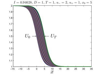
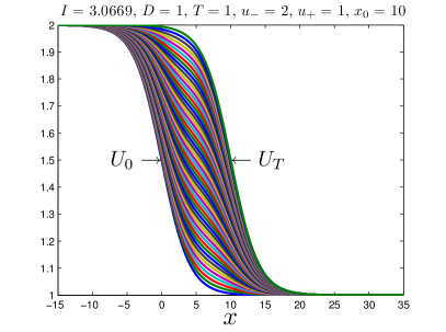
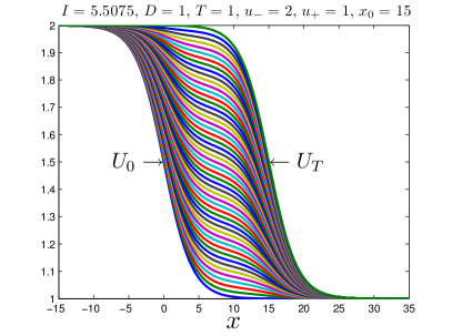
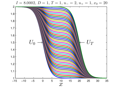
Fig. 1: The optimal paths and their values of $I$ in (40) in the case that $U_{T}(x)=U_{0}(x-x_{0})$ for different $x_{0}$. In each figure, we plot the curves indicating the optimal path at time $0,\Delta t,2\Delta t,\ldots,T=1$. We can see that for $x_{0}$ small, the optimal path is close to the linear shift traveling wave and for $x_{0}$ large, the optimal path looks like the linear interpolation of $U_{0}$ and $U_{T}$. These observations are consistent with the test function $v$ and $w$ we use for the upper bounds in Section 5.2 and 5.3.

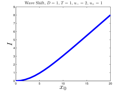
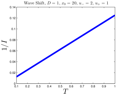
Fig. 2: Left: The optimal values of $I$ in (40) versus $x_{0}$ in the case that $U_{T}(x)=U_{0}(x-x_{0})$ for $x_{0}=0,1,2,\ldots,20$ with the same setting in Fig.1. We see that the curve is quadratic for $x_{0}$ small and linear for $x_{0}$ large (see (23)). Right: The reciprocal of the optimal values of $I$ in (40) versus $T$ in the case that $U_{T}(x)=U_{0}(x-x_{0})$ for $x_{0}=20$ and $T=0.1,0.2,\ldots,1$ with the same setting in Fig.1. We see that the curve is linear in $T$, which means the optimal $I$ is of $\Theta(1/T)$ (see also (23)).

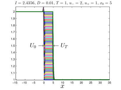
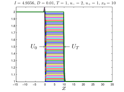
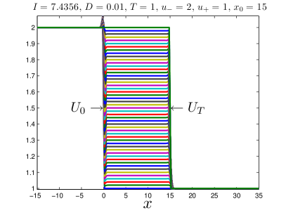
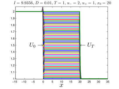
Fig. 3: The optimal paths and their values of $I$ in (40) in the case that $U_{T}(x)=U_{0}(x-x_{0})$ for different $x_{0}$. In each figure, we plot the curves indicating the optimal path at time $0,\Delta t,2\Delta t,\ldots,T=1$. Different from Fig.1, as the transition region is very small, we see nearly no shifted part but only the linear interpolation.

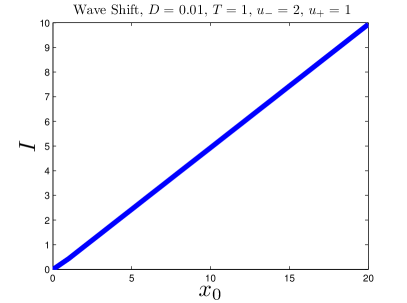
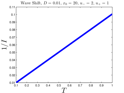
Fig. 4: Left: The optimal values of $I$ in (40) versus $x_{0}$ in the case that $U_{T}(x)=U_{0}(x-x_{0})$ for $x_{0}=0,1,2,\ldots,20$ with the same setting in Fig.3. As what we see in Fig.3, the optimal path is the linear interpolation and thus the curves is almost linear except a small perturbation around $x_{0}=0$. Right: The reciprocal of the optimal values of $I$ in (40) versus $T$ in the case that $U_{T}(x)=U_{0}(x-x_{0})$ for $T=0.1,0.2,\ldots,1$ with the same setting in Fig.3. We see that the curve is linear in $T$, which means the optimal $I$ is $\mathcal{O}(1/T)$.

6.5 Change of wave speeds

In this subsection we consider the rare event in which $u(0,x)=U_{0}(x)$ and $u(T,x)=U_{T}(x):=U_{1}(x)$ because of $\varepsilon\dot{W}$, where $U_{1}(x)$ is a traveling wave with $u_{1\pm}:=\lim_{x\to\pm\infty}U_{1}(x)$ which are different from $u_{\pm}=\lim_{x\to\pm\infty}U_{0}(x)$, and such that $\gamma_{1}=\frac{F(u_{1+})-F(u_{1-})}{u_{1+}-u_{1-}}$ is different from $\gamma=\frac{F(u_{+})-F(u_{-})}{u_{+}-u_{-}}$. This case does not belong to the class of problems addressed in the previous sections of this paper, in which the boundary conditions are fixed. But it is still possible to look for the optimal paths going from $U_{0}$ to $U_{T}$ and that minimize the rate function $I$.

The boundary conditions are more delicate to implement in this case. We know that $U_{0}$ and $U_{T}$ are very close to constants when $L$ and $R$ are far from their transition regions. In this case, the LDP implies that the optimal path around the boundaries should be very close to the linear interpolations of $U_{0}$ and $U_{T}$ in time. Therefore we let:

$$q_{1}^{n}=(1-\frac{n}{N})q_{1}^{0}+\frac{n}{N}q_{1}^{N},\quad q_{M}^{n}=(1-\frac{n}{N})q_{M}^{0}+\frac{n}{N}q_{M}^{N}.$$

It is possible not to set the boundary conditions and to optimize the boundary cells as well. Our numerical simulations show, however, that the solution in both cases is basically the same except for some oscillations near the boundaries. The oscillations come from the inappropriate discretization at the boundaries, and this is a limitation of the numerical discretization. We can have a few extra boundary conditions to reduce the unwanted oscillations at the boundaries. For example, we can additionally set

$$q_{2}^{n}=(1-\frac{n}{N})q_{2}^{0}+\frac{n}{N}q_{2}^{N},\quad q_{M-1}^{n}=(1-\frac{n}{N})q_{M-1}^{0}+\frac{n}{N}q_{M-1}^{N}.$$

The results are shown in Fig.5. We let $\gamma=0$ and $\gamma_{1}=3.5$ while we keep $u_{-}-u_{+}=u_{1-}-u_{1+}=1$ to indicate that $U_{0}$ and $U_{T}$ have roughly the same transition magnitude. We see that the values of the rate function are much larger than that of the anomalous wave displacements. This means that it is very unlikely to have changes of wave speeds compared to wave displacements.

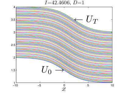
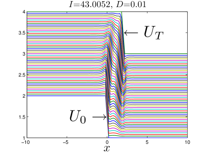
Fig. 5: The optimal paths and their values of $I$ in (40) in the case that $U_{0}$ and $U_{T}$ have different speeds. Here we let $\gamma=1.5$ in Burgers’ equation (41), and therefore the speed of $U_{0}$ is zero and the speed of $U_{T}$ is $3.5$. The differences between the left and right boundary values are kept the same so that $U_{0}$ and $U_{T}$ have the same transition magnitude. In each figure, we plot the curves indicating the optimal path at time $0,\Delta t,2\Delta t,\ldots,T=1$.

6.6 Weak shocks to strong shocks and strong shocks to weak shocks

We also consider the case that $U_{0}$ is a weak (strong) shock while $U_{T}$ is a strong (weak) shock. By a strong shock we mean that the difference between $u_{-}$ and $u_{+}$ is large. This case is also not in the range of our analytical framework, but we can still compute the rate function after we impose the suitable boundary conditions. We use the same boundary conditions as the ones in the previous subsection:

$$q_{1}^{n}=(1-\frac{n}{N})q_{1}^{0}+\frac{n}{N}q_{1}^{N},\quad q_{M}^{n}=(1-\frac{n}{N})q_{M}^{0}+\frac{n}{N}q_{M}^{N},$$

$$q_{2}^{n}=(1-\frac{n}{N})q_{2}^{0}+\frac{n}{N}q_{2}^{N},\quad q_{M-1}^{n}=(1-\frac{n}{N})q_{M-1}^{0}+\frac{n}{N}q_{M-1}^{N}.$$

From Fig.6 and Fig.7 we see that the optimal path of weak to strong and the one of strong to weak are significantly different, even if the reference strong and weak shocks are fixed. We note the very large value of the rate function compared to anomalous displacement, and how it depends on $D$. This confirms quantitatively the expectation that shock profiles are very stable and they are not easily perturbed except for displacements.

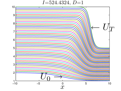
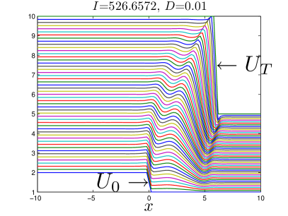
Fig. 6: The optimal paths and their values of $I$ in (40) in the case that $U_{0}$ is a weak shock while $U_{T}$ is a strong shock. Here we let $U_{0}$ has a small difference in the boundary values while $U_{T}$ has a large one. In each figure, we plot the curves indicating the optimal path at time $0,\Delta t,2\Delta t,\ldots,T=1$.

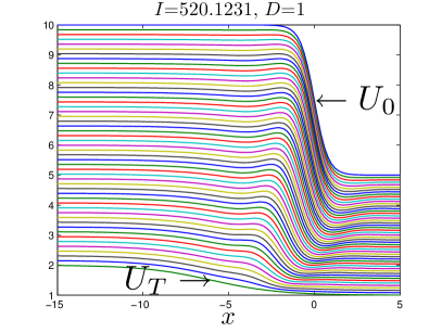
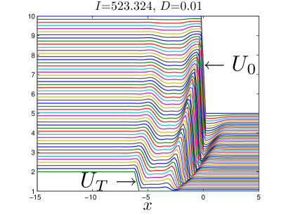
Fig. 7: The optimal paths and their values of $I$ in (40) in the case that $U_{0}$ is a strong shock while $U_{T}$ is a weak shock. Here we let $U_{0}$ has a large difference in the boundary values while $U_{T}$ has a small one. In each figure, we plot the curves indicating the optimal path at time $0,\Delta t,2\Delta t,\ldots,T=1$.

7 Direct numerical simulations with importance sampling

The large deviations probabilities calculated in Sections 5 and 6 are only the exponential decay rates of the probabilities but not the actual probabilities. In this section we use Monte Carlo methods to compute the actual probabilities numerically.

7.1 Burgers’ equation with spatially correlated random perturbations

We reformulate the discretized problem for Burgers’ equation when we have spatially correlated random perturbations. Given a traveling wave solution $U_{0}(x-\gamma t)$ of Burgers’ equation with $\lim_{x\to\pm\infty}U_{0}(x)=u_{\pm}$, we transform to moving coordinates

$$u_{t}+\Big{(}\frac{1}{2}(u-\gamma)^{2}\Big{)}_{x}=(Du_{x})_{x}+\varepsilon\dot{W}.$$ (46)

Then $U_{0}(x)$ is a stationary traveling wave of (46). The rare event we consider is

$$A_{\delta}=\{u\in{\cal E}^{1}\mbox{ such that }u(0,\cdot)=U_{0},\,\|u(T,\cdot)-U_{0}(\cdot-x_{0})\|_{L^{2}}\leq\delta\}.$$

Although for a discrete conservation law it is also possible to consider the other cases in Section 6, their probabilities are too small to compute by the basic Monte Carlo method so we omit them.

To compute $\mathbb{P}(u\in A_{\delta})$ numerically, we discretize the space and time domains uniformly as in Section 6.1: $L=x_{0}<\cdots<x_{M}=R$, $M\Delta x=R-L$ and $0=t_{0}<\cdots<t_{N}=T$, $N\Delta t=T$. Here $Q_{m}^{n}$ denotes the average of $u$ over the $m$-th cell at time $n\Delta t$, and evolves by the Euler method:

$$Q_{m}^{n+1}=Q_{m}^{n}-\frac{\Delta t}{\Delta x}(F_{m+\frac{1}{2}}^{n}-F_{m-\frac{1}{2}}^{n})+D\frac{\Delta t}{\left(\Delta x\right)^{2}}(Q_{m+1}^{n}-2Q_{m}^{n}+Q_{m-1}^{n})+\varepsilon\Delta W_{m}^{n},$$ (47)

for $m=2,\ldots,M-1$, $n=1,\ldots,N$, where $F_{m\pm 1/2}^{n}(Q^{n})$ are numerical fluxes of $(u-\gamma)^{2}/2$ constructed by Godunov’s method and $(\Delta W_{m}^{n})_{m=2,\ldots,M-1,n=1,\ldots,N}$ are Gaussian random variables with mean $0$ and covariance

$$\mathbb{E}(\Delta W_{m_{1}}^{n_{1}}\Delta W_{m_{2}}^{n_{2}})=\begin{cases}\frac{\Delta t}{\Delta x}C_{m_{1}m_{2}},\quad&n_{1}=n_{2},\\ 0,\quad&\text{otherwise.}\end{cases}$$

In order to make the problem more realistic, we assume that the variables $\Delta W_{m}^{n}$ are spatially correlated: $C_{m_{1}m_{2}}=\sigma^{2}\exp(-\frac{1}{l_{c}}|x_{m_{1}}-x_{m_{2}}|)$ and $C=(C_{ij})_{i,j=2}^{M-1}=\Phi\Phi^{T}$. Finally we impose the initial and boundary conditions: $Q_{m}^{0}=U_{0}(x_{m-1/2})$, $Q_{1}^{n}=u_{-}$ and $Q_{M}^{n}=u_{+}$.

7.2 Introduction to importance sampling

To estimate $\mathbb{P}(u\in A_{\delta})$, we may use the basic Monte Carlo method. The Monte Carlo strategy is as follows. We generate $K$ independent samples $\Delta W^{(k)}=(\Delta W_{m}^{n,(k)})_{m=2,\ldots,M-1,n=1,\ldots,N}$, $k=1,\ldots,K$, of the Gaussian vector $(\Delta W_{m}^{n})_{m=2,\ldots,M-1,n=1,\ldots,N}$, which give $K$ independent samples $Q^{(k)}=(Q_{m}^{n,(k)})_{m=1,\ldots,M,n=1,\ldots,N}$, $k=1,\ldots,K$ of the random vector $Q=(Q_{m}^{n})_{m=1,\ldots,M,n=1,\ldots,N}$. The basic Monte Carlo estimator is

$$\hat{P}^{MC}=\frac{1}{K}\sum_{k=1}^{K}1_{A_{\delta}}(Q^{(k)})$$ (48)

where

$$Q\in A_{\delta}\mbox{ if and only if }\Delta x\sum_{m=1}^{M}[Q_{m}^{N}-U_{0}(x_{m-\frac{1}{2}}-x_{0})]^{2}\leq\delta^{2}.$$ (49)

In other words, $\hat{P}^{MC}$ is the empirical frequency that $Q^{(k)}\in A_{\delta}$. It is an unbiased estimator $\mathbb{E}[\hat{P}^{MC}]=\mathbb{P}(Q\in A_{\delta})$. By the law of large numbers, it is strongly convergent $\hat{P}^{MC}\to\mathbb{P}(Q\in A_{\delta})$ almost surely as $K\to\infty$. Its variance is given by

$$\mathbf{Var}(\hat{P}^{MC})=\frac{1}{K}\mathbf{Var}(1_{A_{\delta}}(Q))=\frac{1}{K}\big{(}\mathbb{P}(Q\in A_{\delta})-\mathbb{P}(Q\in A_{\delta})^{2}\big{)}.$$

In order to have a meaningful estimation, the standard deviation of the estimator and $\mathbb{P}(Q\in A_{\delta})$ should be of the same order. Namely, the relative error

$$\frac{\mathbf{Var}^{\frac{1}{2}}(\hat{P}^{MC})}{\mathbb{P}(Q\in A_{\delta})}=\frac{1}{\sqrt{K}}\left(\frac{1}{\mathbb{P}(Q\in A_{\delta})}-1\right)^{\frac{1}{2}}$$

should be of order one (or smaller). This means that the number $K$ of Monte Carlo samples should be at least of the order of the reciprocal of the probability $\mathbb{P}(Q\in A_{\delta})$. We note that for $\varepsilon$ small, $\mathbb{P}(Q\in A_{\delta})$ decreases exponentially and so $K$ should be increased exponentially; the exponential growth of $K$ makes the basic Monte Carlo method computationally infeasible.

The well established way to overcome the difficulty of calculating rare event probabilities is to use importance sampling. The problem with basic Monte Carlo is that for small $\varepsilon$ there are very few samples in $A_{\delta}$ under the original measure $\mathbb{P}$ so the estimator is inaccurate. In importance sampling we change the original measure so that there is a significant fraction of $Q^{k}$ in $A_{\delta}$ under this new measure $\mathbb{Q}$, even for small $\varepsilon$. Since we use the biased measure $\mathbb{Q}$ to generate $Q^{(k)}$, it is necessary to weight the simulation outputs in order to get an unbiased estimator of $\mathbb{P}(Q\in A_{\delta})$. The correct weight is the likelihood ratio since we have:

$$\mathbb{P}(Q\in A_{\delta})=\mathbb{E}_{\mathbb{P}}[1_{A_{\delta}}(Q)]=\mathbb{E}_{\mathbb{Q}}\big{[}1_{A_{\delta}}(Q)\frac{d\mathbb{P}}{d\mathbb{Q}}(Q)\big{]}.$$

Then the importance sampling estimator is

$$\hat{P}^{IS}=\frac{1}{K}\sum_{k=1}^{K}1_{A_{\delta}}(Q^{(k)})\frac{d\mathbb{P}}{d\mathbb{Q}}(Q^{(k)}),$$ (50)

where $Q^{(k)}$ are generated under $\mathbb{Q}$. The estimator $\hat{P}^{IS}$ is unbiased $\mathbb{E}_{\mathbb{Q}}[\hat{P}^{IS}]=\mathbb{P}(Q\in A_{\delta})$ and its variance is

$$\mathbf{Var}_{\mathbb{Q}}(\hat{P}^{IS})=\frac{1}{K}\mathbf{Var}_{\mathbb{Q}}\big{(}1_{A_{\delta}}(Q)\frac{d\mathbb{P}}{d\mathbb{Q}}(Q)\big{)}$$

The main issue in importance sampling is how to choose a good $\mathbb{Q}$ to have a low $\mathbf{Var}_{\mathbb{Q}}[1_{A_{\delta}}(Q)\frac{d\mathbb{P}}{d\mathbb{Q}}(Q)]$. In many cases (see for example, [22, 21, 3, 20]), it can be shown that the change of measure suggested by the most probable path of the LDP is asymptotically optimal as $\varepsilon\to 0$. However, it is also well-known that in some cases (see [12]), the estimator by this strategy is worse than the basic Monte Carlo, and may even have infinite variance. However, because the rare event $A_{\delta}$ is convex and the discrete rate function $I$ is (numerically tested) essentially convex, the importance sampling estimator by this strategy is expected to be asymptotically optimal and we will see that it indeed works very well.

7.3 Importance sampling based on the most probable path

In this subsection we implement the importance sampling by using a biased distribution centered on the most probable path obtained in Section 6. From Section 6.1, $\bar{Q}:=\arg\inf_{Q\in A_{\delta}}I(Q)$ is the most probable path as $\varepsilon\to 0$ by the large deviation principle. We choose $\bar{h}=(\bar{h}^{n})_{n=1,\ldots,N}=(\bar{h}^{n}_{m})_{m=2,\ldots,M-1,n=1,\ldots,N}$ such that

$$\bar{Q}_{m}^{n+1} =\bar{Q}_{m}^{n}-\frac{\Delta t}{\Delta x}(F_{m+\frac{1}{2}}(\bar{Q}^{n})-F_{m-\frac{1}{2}}(\bar{Q}^{n}))$$ (51)

$$\quad+D\frac{\Delta t}{\left(\Delta x\right)^{2}}(\bar{Q}_{m+1}^{n}-2\bar{Q}_{m}^{n}+\bar{Q}_{m-1}^{n})+(\Phi\bar{h}^{n})_{m},$$

for $m=2,\ldots,M-1$, $n=1,\ldots,N$.

Assume that under the probability $\mathbb{Q}$, the vector $\Delta W^{n}:=(\Delta W^{n}_{m})_{m=2,\ldots,M-1}$ in (47) is multivariate Gaussian $\mathcal{N}(\varepsilon^{-1}\Phi\bar{h}^{n},\frac{\Delta t}{\Delta x}C)$ and $\mathbf{Cov}(\Delta W_{m_{1}}^{n_{1}},\Delta W_{m_{2}}^{n_{2}})=0$ if $n_{1}\neq n_{2}$. Denoting $\Delta W=(\Delta W^{n})_{n=1,\ldots,N}$, the likelihood ratio $d\mathbb{P}/d\mathbb{Q}$ can be computed explicitly:

$$\frac{d\mathbb{P}}{d\mathbb{Q}}(\Delta W)=\exp\left(-\frac{1}{2}\sum_{n=1}^{N}[\|\Phi^{-1}\Delta W^{n}\|_{2}^{2}-\|\Phi^{-1}\Delta W^{n}-\varepsilon^{-1}\bar{h}^{n}\|_{2}^{2}\right).$$ (52)

Note that under $\mathbb{Q}$, (47) can be written as

$$Q_{m}^{n+1}=Q_{m}^{n}-\frac{\Delta t}{\Delta x}(F_{m+\frac{1}{2}}^{n}-F_{m-\frac{1}{2}}^{n})+D\frac{\Delta t}{\left(\Delta x\right)^{2}}(Q_{m+1}^{n}-2Q_{m}^{n}+Q_{m-1}^{n})+(\Phi\bar{h}^{n})_{m}+\varepsilon\Delta\tilde{W}_{m}^{n},$$ (53)

where $\Delta\tilde{W}=(\Delta\tilde{W}_{m}^{n})_{m=2,\ldots,M-1,n=1,\ldots,N}$ is zero-mean, Gaussian with the spatial covariance $\frac{\Delta t}{\Delta x}C$, and white in time. Then (52) can be written as

$$\frac{d\mathbb{P}}{d\mathbb{Q}}(\Delta\tilde{W})=\exp\left(-\frac{1}{2}\sum_{n=1}^{N}\|\Phi^{-1}\Delta\tilde{W}^{n}+\varepsilon^{-1}\bar{h}^{n}\|_{2}^{2}-\|\Phi^{-1}\Delta\tilde{W}^{n}\|_{2}^{2}\right).$$ (54)

In summary, the importance sampling Monte Carlo strategy is implemented as follows:

1. Compute the optimal path $\bar{Q}=\arg\inf_{Q\in A_{\delta}}I(Q)$ and its residual $\bar{h}$ from (51).

2. Sample $K$ independent $\Delta\tilde{W}^{(k)}$ with the zero-mean, Gaussian distribution with the covariance $\frac{\Delta t}{\Delta x}C$ in space and white in time. Compute the corresponding $Q^{(k)}$ by (53).

3. The importance sampling estimator is

   $$\hat{P}^{IS}=\frac{1}{K}\sum_{k=1}^{K}1_{A_{\delta}}(Q^{(k)})\frac{d\mathbb{P}}{d\mathbb{Q}}(\Delta\tilde{W}^{(k)}),$$

   where $\frac{d\mathbb{P}}{d\mathbb{Q}}(\Delta\tilde{W})$ is defined in (54).

7.4 Simulations with importance sampling

We consider three estimators: the basic Monte estimator $\hat{P}^{MC}$ and two importance sampling estimators: $\hat{P}^{IS}_{0}$ and $\hat{P}^{IS}_{\delta}$, where $\hat{P}^{IS}_{0}$ uses $\bar{h}$ in (51) with $\bar{Q}=\arg\inf_{Q\in A_{0}}I(Q_{m}^{n})$ while $\hat{P}^{IS}_{\delta}$ uses $\bar{h}$ in (51) with $\bar{Q}=\arg\inf_{Q\in A_{\delta}}I(Q)$. The parameters for the simulations are listed in Table 1.

$\Delta x=0.5$	$\Delta t=0.05$	$L=-15$	$R=20$	$T=1$	$u_{-}=2$	$u_{+}=1$
$\gamma=1.5$	$D=1$	$x_{0}=5$	$\delta=\sqrt{0.5}$	$\sigma=1$	$l_{c}=5$	$K=10^{4}$

Table 1: The parameters for the Monte Carlo simulations.

As we mention before, we only test the wave displacement with $x_{0}=5$ and $D=1$ because the probabilities of the other cases in Section 6 are too small for $\hat{P}^{MC}$ to have meaningful samples.

First we find the optimal paths for $\inf_{Q\in A_{0}}I(Q)$ and $\inf_{Q\in A_{\delta}}I(Q)$. As before, $\inf_{Q\in A_{0}}I(Q)$ can be modeled as an unconstrained optimization problem and we solve it by the BFGS method while we solve $\inf_{Q\in A_{\delta}}I(Q)$ by sequential quadratic programming (SQP) [19].

From Fig.8 we note that $\inf_{Q\in A_{0}}I(Q)$ is much smaller than the corresponding one with spatially white noise. This is because with the correlated noise, it is easier to have simultaneous increments. In addition, $\inf_{Q\in A_{\delta}}I(Q)$ is significantly different from $\inf_{Q\in A_{0}}I(Q)$ because $\delta=\sqrt{0.5}$ is not very small. we will see that this difference significantly affects the performances of $\hat{P}^{IS}_{0}$ and $\hat{P}^{IS}_{\delta}$.

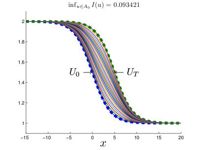
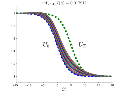
Fig. 8: The optimal paths for $\inf_{Q\in A_{0}}I(Q)$ and $\inf_{Q\in A_{\delta}}I(Q)$. With the spatially correlated noise, $\inf_{Q\in A_{0}}I(Q)$ is much lower than the one with the spatially white noise (see Fig.1).

Once $\arg\inf_{Q\in A_{0}}I(Q)$ and $\arg\inf_{Q\in A_{\delta}}I(Q)$ are obtained, we can construct $\hat{P}^{IS}_{0}$ and $\hat{P}^{IS}_{\delta}$. We estimate $\mathbb{P}(Q\in A_{\delta})$ by these three estimators for $100$ different $\varepsilon$ taken uniformly in $[0.01,0.2]$. For each $\varepsilon$ and estimator, we use $K=10^{4}$ samples. The (numerical) $99\%$ confidence intervals are defined by $\big{[}{\rm Mean}_{K}-2.6\,{\rm Std}_{K},{\rm Mean}_{K}+2.6\,{\rm Std}_{K}\big{]}$ where the (numerical) mean and standard deviation are

$${\rm Mean}_{K}=\frac{1}{K}\sum_{k=1}^{K}p^{(k)},\quad\quad{\rm Std}_{K}^{2}=\frac{1}{K}\sum_{k=1}^{K}(p^{(k)})^{2}-{\rm Mean}_{K}^{2},$$

with $p^{(k)}={\bf 1}_{A_{\delta}}(Q^{(k)})$ for $\hat{P}^{MC}$ and $p^{(k)}=d\mathbb{P}/d\mathbb{Q}(\Delta\tilde{W}^{(k)}){\bf 1}_{A_{\delta}}(Q^{(k)})$ for $\hat{P}^{IS}$. We find that $\hat{P}^{IS}_{\delta}$ has the best performance and $\hat{P}^{IS}_{0}$ also has the good performance for $0.1\leq\varepsilon\leq 0.2$. For $\epsilon<0.1$, because $\arg\inf_{Q\in A_{0}}I(Q)$ is not the optimal path, $\hat{P}^{IS}_{0}$ is even worse than $\hat{P}^{MC}$ due to the inappropriate change of measure. For $\epsilon<0.1$, because $\arg\inf_{Q\in A_{\delta}}I(Q)$ is the optimal path, $\hat{P}^{IS}_{\delta}$ dramatically outperforms $\hat{P}^{MC}$. This shows that large-deviations-driven importance sampling strategies can be efficient to estimate rare event probabilities in the context of perturbed scalar conservation laws.

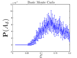
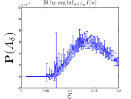
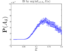
Fig. 9: The estimated probabilities and their $99\%$ confidence intervals by $\hat{P}^{MC}$, $\hat{P}^{IS}_{0}$ and $\hat{P}^{IS}_{\delta}$. $\hat{P}^{IS}_{\delta}$ has the best performance and $\hat{P}^{IS}_{0}$ also has the good performance for $0.1\leq\varepsilon\leq 0.2$. However $\hat{P}^{IS}_{0}$ works poorly for $\epsilon<0.1$.

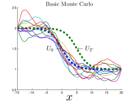
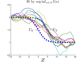
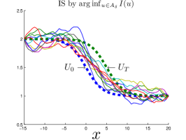
Fig. 10: Sample paths under these three probability measures with $\varepsilon=0.1$.

We plot the estimated probabilities and the relative error, the ratio of the (numerical) standard deviation to the (numerical) mean, in the log scale. Note that in the extreme case, the estimated probability is dominated by the value $p^{(k_{0})}$ of one realization over $K$ ($p^{(k_{0})}=1$ for $\hat{P}^{MC}$ and $p^{(k_{0})}=d\mathbb{P}/d\mathbb{Q}(\Delta\tilde{W}^{(k_{0})})$ for $\hat{P}^{IS}$), and the numerical variance is approximately $(p^{(k_{0})})^{2}/K$. Therefore the relative error is about $\sqrt{K}=100$. This is why the curves of the relative errors in Fig.11 saturate at $100$, and it also tells us that when the relative error reaches $\sqrt{K}$, the estimator is in the extreme case and so is not reliable.

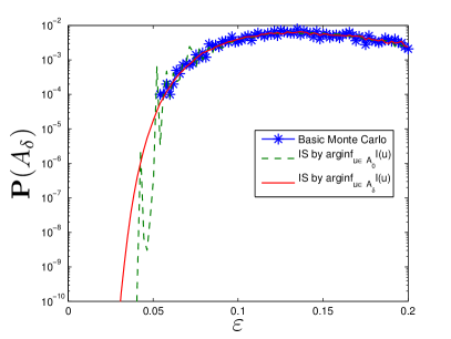
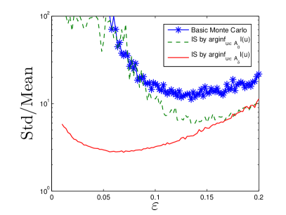
Fig. 11: The semilog plots of the estimated probabilities (left) and the relative errors (right).

8 Conclusion and open problems

We have analyzed here the small probabilities of anomalous shock profile displacements due to random perturbations using the theory of large deviations. We have obtained analytically upper and lower bounds for the exponential rate of decay of these probabilities and we have verified the accuracy of these bounds with numerical simulations. We have also used Monte Carlo simulations with importance sampling based on the analytically known rate function, which is efficient and gives very good results for rare event probabilities.

Appendix A Proof of Lemma 2

Taking a Fourier transform in $x$ we have

$$\hat{Z}(t,\xi)=\int_{0}^{t}e^{-D\xi^{2}(t-s)}d\hat{W}(s,\xi),$$

where $\hat{W}(t,\xi)=\int W(t,x)e^{-i\xi x}dx$ is a complex Gaussian process with mean zero and covariance

$$\mathbb{E}\big{[}\hat{W}(t,\xi)\overline{\hat{W}(t^{\prime},\xi^{\prime})}\big{]}=t\wedge t^{\prime}\,\hat{C}(\xi,\xi^{\prime}),$$

with $\hat{C}(\xi,\xi^{\prime})=\int e^{-i\xi x+i\xi^{\prime}x^{\prime}}C(x,x^{\prime})dxdx^{\prime}$. We find that

$$\mathbb{E}[|\hat{Z}(t,\xi)|^{2}]=\frac{1-e^{-2D\xi^{2}t}}{2D\xi^{2}}\hat{C}(\xi,\xi).$$

On the one hand, the fact that $\Phi$ is Hilbert-Schmidt from $L^{2}$ into $L^{2}$ implies that

$$\int\hat{C}(\xi,\xi)d\xi=2\pi\|\Phi(\cdot,\cdot)\|_{L^{2}(\mathbb{R}\times\mathbb{R})}^{2}$$

is finite. On the other hand we have $(1-e^{-s})/s\leq 1$ uniformly with respect to $s\in(0,\infty)$, so we get that for any $t\in[0,T]$

$$\int(1+\xi^{2})\mathbb{E}[|\hat{Z}(t,\xi)|^{2}]d\xi\leq 2\pi\big{(}T+\frac{1}{2D}\big{)}\|\Phi(\cdot,\cdot)\|_{L^{2}(\mathbb{R}\times\mathbb{R})}^{2},$$

which is equivalent by Parseval relation to

$$\mathbb{E}[\|{Z}(t)\|_{H^{1}}^{2}]\leq\big{(}T+\frac{1}{2D}\big{)}\|\Phi(\cdot,\cdot)\|_{L^{2}(\mathbb{R}\times\mathbb{R})}^{2},$$

which gives that $Z(t)\in L^{2}([0,T],H^{1}(\mathbb{R}))$ almost surely. Similarly we find

$$\mathbb{E}\big{[}|\hat{Z}(t,\xi)-\hat{Z}(t^{\prime},\xi)|^{2}\big{]} = \big{[}1-e^{-D\xi^{2}|t-t^{\prime}|}\big{]}\big{[}2-e^{-2D\xi^{2}t\wedge t^{\prime}}+e^{-D\xi^{2}(t+t^{\prime})}\big{]}\frac{\hat{C}(\xi,\xi)}{2D\xi^{2}}$$

$$\leq \big{[}1-e^{-D\xi^{2}|t-t^{\prime}|}\big{]}\frac{\hat{C}(\xi,\xi)}{D\xi^{2}}\leq|t-t^{\prime}|\hat{C}(\xi,\xi),$$

which gives

$$\mathbb{E}\big{[}\|Z(t)-Z(t^{\prime})\|_{L^{2}}^{4}\big{]}=\iint\mathbb{E}\big{[}|Z(t,x)-Z(t^{\prime},x)|^{2}|Z(t,x^{\prime})-Z(t^{\prime},x^{\prime})|^{2}\big{]}dxdx^{\prime}$$

$$\leq\iint\mathbb{E}\big{[}|Z(t,x)-Z(t^{\prime},x)|^{4}\big{]}^{1/2}\mathbb{E}\big{[}|Z(t,x^{\prime})-Z(t^{\prime},x^{\prime})|^{4}\big{]}^{1/2}dxdx^{\prime}$$

$$=3\iint\mathbb{E}\big{[}|Z(t,x)-Z(t^{\prime},x)|^{2}\big{]}\mathbb{E}\big{[}|Z(t,x^{\prime})-Z(t^{\prime},x^{\prime})|^{2}\big{]}dxdx^{\prime}$$

$$=3\Big{(}\int\mathbb{E}\big{[}|Z(t,x)-Z(t^{\prime},x)|^{2}\big{]}dx\Big{)}^{2}\leq 3(2\pi)^{2}|t-t^{\prime}|^{2}\|\Phi(\cdot,\cdot)\|_{L^{2}(\mathbb{R}\times\mathbb{R})}^{4},$$

where we have used the fact that ${Z}(t,x)-Z(t^{\prime},x)$ is a Gaussian random variable and Parseval equality. By Kolmogorov’s continuity criterium for Hilbert valued stochastic processes [4, Theorem 3.3] we find that that $Z(t)\in{\cal C}([0,T],L^{2}(\mathbb{R}))$ almost surely.

If $\Phi$ is Hilbert-Schmidt from $L^{2}$ into $H^{1}$, then

$$\int\xi^{2}\hat{C}(\xi,\xi)d\xi=2\pi\|\partial_{x}\Phi(\cdot,\cdot)\|_{L^{2}(\mathbb{R}\times\mathbb{R})}^{2}$$

is finite, and we can repeat the same arguments to show the final result.

Appendix B Proofs in Section 3

B.1 Proof of Propsition 4

From Lemma 2, $Z(t)=\int_{0}^{t}S(t-s)dW(s)$ is in $\mathcal{C}([0,T],H^{1}(\mathbb{R}))$ almost surely. We want to prove the existence and uniqueness in ${\cal E}^{1}$ of the solution to the equation

$$u(t)=S(t)U-\int_{0}^{t}S(t-s)[F(u(s))]_{x}ds+\varepsilon Z(t),$$ (55)

where $F$ is a $\mathcal{C}^{2}$ function with $\max\{\|F^{\prime}\|_{L^{\infty}},\|F^{\prime\prime}\|_{L^{\infty}}\}\leq C_{F}<\infty$.

To prove the existence we use the Picard iteration scheme: we define $u^{0}(t)\equiv U$ and

$$u^{n+1}(t)=S(t)U-\int_{0}^{t}S(t-s)[F(u^{n}(s))]_{x}ds+\varepsilon Z(t).$$

Therefore,

$$u^{n+1}(t)-U =S(t)U-U-\int_{0}^{t}S(t-s)[F^{\prime}(u^{n}(s))(u_{x}^{n}(s)-U_{x})]ds$$ (56)

$$\quad-\int_{0}^{t}S(t-s)[F^{\prime}(u^{n}(s))U_{x}]ds+\varepsilon Z(t).$$

It is easy to see that $u^{n}(t)-U\in\mathcal{C}([0,T],H^{1}(\mathbb{R}))$ for all $n$, and we first show that $\sup_{t\in[0,T]}\|u^{n}(t)-U\|_{H^{1}(\mathbb{R})}$ are uniformly bounded in $n$.

Lemma 20.

Let $a_{n}(t)=\|u^{n}(t)-U\|_{H^{1}}$. Then there exists a constant $C_{u}$ such that $a_{n}(t)\leq C_{u}$ for all $n$ and $t\in[0,T]$. As a consequence, we can choose sufficiently large $C_{u}$ such that $\|u^{n}_{x}(t)\|_{L^{2}}\leq C_{u}$ for all $n$ and $t\in[0,T]$.

Proof.

Note that $\sup_{t\in[0,T]}\|S(t)U-U\|_{H^{1}}$ and $\sup_{t\in[0,T]}\|\varepsilon Z(t)\|_{H^{1}}$ are bounded. In addition, by [23, Chap. 15, Sec. 1], $\|S(t-s)\|_{\mathcal{L}(L^{2},H^{1})}=\mathcal{O}((t-s)^{-1/2})$, then

$$\left\|\int_{0}^{t}S(t-s)[F^{\prime}(u^{n}(s))U_{x}]ds\right\|_{H^{1}} \leq\int_{0}^{t}\|S(t-s)\|_{\mathcal{L}(L^{2},H^{1})}\|F^{\prime}(u^{n}(s))U_{x}\|_{L^{2}}ds$$

$$\leq C_{F}\|U_{x}\|_{L^{2}}\int_{0}^{t}\|S(t-s)\|_{\mathcal{L}(L^{2},H^{1})}ds,$$

are uniformly bounded in $n$, and

$$\left\|\int_{0}^{t}S(t-s)[F^{\prime}(u^{n}(s))(u_{x}^{n}(s)-U_{x})]ds\right\|_{H^{1}}$$

$$\quad\leq\int_{0}^{t}\|S(t-s)\|_{\mathcal{L}(L^{2},H^{1})}\|F^{\prime}(u^{n}(s))(u_{x}^{n}(s)-U_{x})\|_{L^{2}}ds$$

$$\quad\leq C_{F}\int_{0}^{t}\|S(t-s)\|_{\mathcal{L}(L^{2},H^{1})}\|u_{x}^{n}(s)-U_{x}\|_{L^{2}}ds$$

$$\quad\leq C_{F}\int_{0}^{t}\|S(t-s)\|_{\mathcal{L}(L^{2},H^{1})}\|u^{n}(s)-U\|_{H^{1}}ds$$

$$\quad\leq C_{F}\left[\int_{0}^{t}\|S(t-s)\|_{\mathcal{L}(L^{2},H^{1})}^{p}ds\right]^{1/p}\left[\int_{0}^{t}\|u^{n}(s)-U\|_{H^{1}}^{q}ds\right]^{1/q}.$$

By letting $1/p+1/q=1$ with $1<p<2$ and $q>2$, we can have the following recursive inequality with a sufficiently large $C$:

$$a_{n+1}(t)\leq\frac{C}{2}+\frac{C}{2}\left[\int_{0}^{t}a_{n}^{q}(s)ds\right]^{1/q}.$$

By the convexity of $x\mapsto x^{q}$,

$$a_{n+1}^{q}(t)\leq\left(\frac{C}{2}+\frac{C}{2}\left[\int_{0}^{t}a_{n}^{q}(s)ds\right]^{1/q}\right)^{q}\leq\frac{C^{q}}{2}+\frac{C^{q}}{2}\int_{0}^{t}a_{n}^{q}(s)ds.$$ (57)

By noting that $a_{0}(t)=0$ and (57), it easy to see that $a_{n}^{q}(t)$ are uniformly bounded in $n$ and $t\in[0,T]$ and so are $a_{n}(t)$. ∎

To prove the convergence of $u^{n}(t)-U$ in $\mathcal{C}([0,T],H^{1}(\mathbb{R}))$, it suffices to prove that $\sum_{n=0}^{\infty}\sup_{t\in[0,T]}\|u^{n+1}(t)-u^{n}(t)\|_{H^{1}}<\infty$.

Lemma 21.

Let $b_{n}(t)=\|u^{n}(t)-u^{n-1}(t)\|_{H^{1}}$. Then $\sum_{n=0}^{\infty}\sup_{t\in[0,T]}b_{n}(t)<\infty$. As a consequence, $u^{n}(t)-U$ converges to $u(t)-U$ in $\mathcal{C}([0,T],H^{1}(\mathbb{R}))$ as $n\to\infty$ and $u(t)$ solves (55).

Proof.

By noting (55), Lemma 20 and $\|\cdot\|_{L^{\infty}}\leq C_{S}\|\cdot\|_{H^{1}}$ (the Sobolev embedding), we have

$$\|u^{n+1}(t)-u^{n}(t)\|_{H^{1}}$$

$$\leq\int_{0}^{t}\|S(t-s)\|_{\mathcal{L}(L^{2},H^{1})}\|F^{\prime}(u^{n}(s))[u_{x}^{n}(s)-u_{x}^{n-1}(s)]\|_{L^{2}}ds$$

$$\quad+\int_{0}^{t}\|S(t-s)\|_{\mathcal{L}(L^{2},H^{1})}\|u_{x}^{n-1}(s)[F^{\prime}(u^{n}(s))-F^{\prime}(u^{n-1}(s))]\|_{L^{2}}ds$$

$$\leq C_{F}\int_{0}^{t}\|S(t-s)\|_{\mathcal{L}(L^{2},H^{1})}\|u^{n}(s)-u^{n-1}(s)\|_{H^{1}}ds$$

$$\quad+\int_{0}^{t}\|S(t-s)\|_{\mathcal{L}(L^{2},H^{1})}\|u_{x}^{n-1}(s)\|_{L^{2}}\|F^{\prime}(u^{n}(s))-F^{\prime}(u^{n-1}(s))\|_{L^{\infty}}ds$$

$$\leq C_{F}\int_{0}^{t}\|S(t-s)\|_{\mathcal{L}(L^{2},H^{1})}\|u^{n}(s)-u^{n-1}(s)\|_{H^{1}}ds$$

$$\quad+C_{F}C_{S}C_{u}\int_{0}^{t}\|S(t-s)\|_{\mathcal{L}(L^{2},H^{1})}\|u^{n}(s)-u^{n-1}(s)\|_{H^{1}}ds$$

$$\leq C_{F}(1+C_{S}C_{u})\left[\int_{0}^{t}\|S(t-s)\|_{\mathcal{L}(L^{2},H^{1})}^{p}ds\right]^{1/p}\left[\int_{0}^{t}\|u^{n}(s)-u^{n-1}(s)\|_{H^{1}}^{q}ds\right]^{1/q},$$

where $1/p+1/q=1$ with $1<p<2$ and $q>2$. Then there exists a constant $C$ such that

$$b_{n+1}^{q}(t)\leq C\int_{0}^{t}b_{n}^{q}(s)ds.$$

Then $b_{n}^{q}(t)\leq b_{0}^{q}(t)C^{n}T^{n}/n!$ so $b_{n}(t)\leq b_{0}(t)(C^{n}T^{n}/n!)^{1/q}$ and it is easy to see that $\sum_{n=0}^{\infty}\sup_{t\in[0,T]}b_{n}(t)<\infty$. ∎

Finally we show that (55) has a unique solution in ${\cal E}^{1}$.

Lemma 22.

If $u,v\in{\cal E}^{1}$ solve (55), then $\sup_{t\in[0,T]}\|u(t)-v(t)\|_{H^{1}}=0$.

Proof.

Let $u,v\in{\cal E}^{1}$ solve (55). Using the same calculations in the proof of Lemma 21, we get

$$\|u(t)-v(t)\|_{H^{1}}\leq C_{F}(1+C_{S}C_{u})\int_{0}^{t}\|S(t-s)\|_{\mathcal{L}(L^{2},H^{1})}\|u(s)-v(s)\|_{H^{1}}ds.$$

By noting that $\|u(0)-v(0)\|_{H^{1}}=0$, $\sup_{t\in[0,T]}\|u(t)-v(t)\|_{H^{1}}=0$ by Gronwall’s inequality. ∎

B.2 Proof of Proposition 5

The LDP can be obtained following the strategy of [11, 6]. The first step of the proof uses the LDP for the laws of the stochastic convolution $\varepsilon Z$ on the space $\mathcal{C}([0,T],H^{1}(\mathbb{R}))$, where

$$Z(t)=\int_{0}^{t}S(t-s)dW(s).$$

The laws of $\varepsilon Z$ are Gaussian measures and the LDP with a good rate function is a consequence of the general result on LDP for centered Gaussian measures on real Banach spaces [8, 11].

The second step is to prove that the mapping $X(t)\mapsto u(t)-U$ is continuous from $\mathcal{C}([0,T],H^{1}(\mathbb{R}))$ into itself, where

$$u(t)=S(t)U-\int_{0}^{t}S(t-s)(F(u(s)))_{x}ds+\int_{0}^{t}S(t-s)X(s)ds.$$ (58)

Then the LDP for $u^{\varepsilon}$ is obtained by the contraction principle [7].

To prove the continuity of the mapping, given two pairs $(X,u)$ and $(Y,v)$ satisfying (58), we show that $v-u\to 0$ as $Y\to X$ in $\mathcal{C}([0,T],H^{1}(\mathbb{R}))$. By using essentially the same calculations in Lemma 21,

$$\|v(t)-u(t)\|_{H^{1}} \leq C_{F}(1+C_{S}C_{u})\int_{0}^{t}\|S(t-s)\|_{\mathcal{L}(L^{2},H^{1})}\|v(s)-u(s)\|_{H^{1}}ds$$

$$\quad+\int_{0}^{t}\|S(t-s)\|_{\mathcal{L}(H^{1},H^{1})}\|Y(s)-X(s)\|_{H^{1}}ds,$$

where $C_{u}=\sup_{t\in[0,T]}\|u_{x}(t)\|_{L^{2}}$. Noting that $\|S(t-s)\|_{\mathcal{L}(H^{1},H^{1})}=\mathcal{O}(1)$ and $\|S(t-s)\|_{\mathcal{L}(L^{2},H^{1})}=\mathcal{O}((t-s)^{-1/2})$, and by Gronwall’s inequality, there exists a constant $C$ such that for $t\in[0,T]$

$$\|v(t)-u(t)\|_{H^{1}}\leq Ce^{C\int_{0}^{T}(T-s)^{-1/2}ds}\int_{0}^{T}\|Y(s)-X(s)\|_{H^{1}}ds.$$ (59)

Because $\int_{0}^{T}(T-s)^{-1/2}ds<\infty$, $v-u\to 0$ as $Y\to X$ in $\mathcal{C}([0,T],H^{1}(\mathbb{R}))$.

B.3 Proof of Proposition 6

For each $n$, we let $h^{n}\in L^{2}([0,T],L^{2}(\mathbb{R}))$ such that $u=\mathcal{H}[h^{n}]$ and

$$\frac{1}{2}\int_{0}^{T}\|h^{n}(t,\cdot)\|_{L^{2}}^{2}dt-\frac{1}{n}<I(u)\leq\frac{1}{2}\int_{0}^{T}\|h^{n}(t,\cdot)\|_{L^{2}}^{2}dt.$$

Because $u\neq U(x-\gamma t)$, $I(u)>0$. We let $u^{n}$ be the mild solution of

$$u^{n}_{t}+(F(u^{n}))_{x}=(Du^{n}_{x})_{x}+(1-(nI(u))^{-1})^{1/2}\Phi h^{n},$$

$$u^{n}(0,x)=U(x).$$

Then $u^{n}-U\in\mathcal{C}([0,T],H^{1}(\mathbb{R}))$ and

$$I(u^{n})\leq\frac{1}{2}\int_{0}^{T}(1-(nI(u))^{-1})\|h^{n}(t,\cdot)\|_{L^{2}}^{2}dt\leq\frac{1}{2}\int_{0}^{T}\|h^{n}(t,\cdot)\|_{L^{2}}^{2}dt-\frac{1}{n}<I(u).$$

We show that $u^{n}-u\to 0$ in $\mathcal{C}([0,T],H^{1}(\mathbb{R}))$. Let $\alpha^{n}=(1-(nI(u))^{-1})^{1/2}$ and replace $(X,u)$ and $(Y,v)$ by $(u,\Phi h^{n})$ and $(u^{n},\alpha^{n}\Phi h^{n})$ respectively in (59). We have

$$\|u^{n}(t)-u(t)\|_{H^{1}} \leq Ce^{C\int_{0}^{T}(T-s)^{-1/2}ds}\int_{0}^{T}(1-\alpha^{n})\|\Phi\|_{\mathcal{L}(L^{2},H^{1})}\|h^{n}(s)\|_{L^{2}}ds$$

$$\leq 2Ce^{C\int_{0}^{T}(T-s)^{-1/2}ds}(1-\alpha^{n})\|\Phi\|_{\mathcal{L}(L^{2},H^{1})}\left(I(u)+\frac{1}{n}\right).$$

Then $u^{n}-u\to 0$ in $\mathcal{C}([0,T],H^{1}(\mathbb{R}))$ as $\alpha^{n}\to 1$.

Appendix C Proof of Proposition 7

We use the following technical result: If $f\in{\cal C}([0,T],H^{1}(\mathbb{R}))$, then $F(t)=\int_{0}^{t}S(t-s)\partial_{x}f(s)ds$ is such that $\int F(t,x)dx=0$ for any $t\in[0,T]$. Indeed, since $f(s)\in H^{1}$ and $H^{1}\subset L^{\infty}$, we have by integrating by parts:

$$F(t,x)=-\int_{0}^{t}\frac{1}{\sqrt{2\pi(t-s)}}\int\partial_{y}\big{(}e^{-\frac{(x-y)^{2}}{2(t-s)}}\big{)}f(s,y)dyds,$$

so that, for any $a<b$

$$\int_{a}^{b}F(t,x)dx=\int_{0}^{t}\frac{1}{\sqrt{2\pi(t-s)}}\int\big{(}e^{-\frac{(b-y)^{2}}{2(t-s)}}-e^{-\frac{(a-y)^{2}}{2(t-s)}}\big{)}f(s,y)dyds.$$

Let $\delta>0$. There exists $M$ such that $\int_{[-M,M]^{c}}f(s,y)^{2}dy<\delta^{2}$ for any $s\in[0,T]$. We can split the integral in $y$ into two pieces. The integral over $[-M,M]^{c}$ can be bounded by Cauchy-Schwarz inequality so we get

$$\big{|}\int_{a}^{b}F(t,x)dx\big{|}=\frac{\sqrt{2}}{\sqrt[4]{\pi}}\delta+\int_{0}^{t}\frac{1}{\sqrt{2\pi(t-s)}}\int_{-M}^{M}\big{(}e^{-\frac{(b-y)^{2}}{2(t-s)}}+e^{-\frac{(a-y)^{2}}{2(t-s)}}\big{)}f(s,y)dyds,$$

and therefore, by Lebesgue’s theorem

$$\limsup_{a\to-\infty,b\to+\infty}\big{|}\int_{a}^{b}F(t,x)dx\big{|}\leq\frac{\sqrt{2}}{\sqrt[4]{\pi}}\delta.$$

Since $\delta$ is arbitrary we get the desired technical result.

We then find by integrating (56) in $x$ that the center of $u^{\varepsilon}$ is given by (16). With the condition that $C$ is in $L^{1}(\mathbb{R}\times\mathbb{R})$, the last term is proportional to a Brownian motion.

Appendix D Proofs in Section 5

D.1 Proof of Lemma 12

The values of $\sigma$, $L_{0}$ and $l_{c}$ do not affect the result, so in the proof we set $\sigma=L_{0}=l_{c}=1$ and $\Phi^{l_{c}}_{L_{0}}=\Phi$ without loss of generality. $\Phi(x,x^{\prime})$ is Hilbert-Schmidt from $L^{2}$ to $H^{k}$ if and only if $\partial_{x}^{j}\Phi(x,x^{\prime})\in L^{2}(\mathbb{R}\times\mathbb{R})$ for $0\leq j\leq k$. Taking the two-dimensional Fourier transform on $\partial_{x}^{j}\Phi(x,x^{\prime})$, we have

$$\mathcal{F}_{\xi,\xi^{\prime}}\{\partial_{x}^{j}\Phi(x,x^{\prime})\} =\mathcal{F}_{\xi}\{\mathcal{F}_{\xi^{\prime}}\{\partial_{x}^{j}\Phi(x,x^{\prime})\}\}=\mathcal{F}_{\xi}\{\partial_{x}^{j}[\phi_{0}(x)\mathcal{F}_{\xi^{\prime}}\{\phi_{1}(x-x^{\prime})\}]\}$$

$$=\mathcal{F}_{\xi}\{\partial_{x}^{j}[\phi_{0}(x)e^{ix\xi^{\prime}}\hat{\phi}_{1}(-\xi^{\prime})\}]\}=(i\xi)^{j}\hat{\phi}_{1}(-\xi^{\prime})\mathcal{F}_{\xi}\{\phi_{0}(x)e^{ix\xi^{\prime}}\}$$

$$=(i\xi)^{j}\hat{\phi}_{1}(-\xi^{\prime})\hat{\phi}_{0}(\xi+\xi^{\prime}).$$

By a simple calculation it is easy to see that $(i\xi)^{j}\hat{\phi}_{1}(-\xi^{\prime})\hat{\phi}_{0}(\xi+\xi^{\prime})\in L^{2}(\mathbb{R}\times\mathbb{R})$ if $\phi_{0}$ and $\phi_{1}$ are both in $H^{j}(\mathbb{R})$.

D.2 Proof of Lemma 13

It suffices to show the case that $\delta_{n}=1/n$. For each $n$, let $u_{n}\in A_{1/n}$, such that $\mathcal{J}(A_{1/n})\leq I(u^{n})<\mathcal{J}(A_{1/n})+1/n$; $\{I(u^{n})\}$ are bounded from above by $\mathcal{J}(A_{1})+1<\infty$. Because $I$ is a good rate function and compactness is equivalent to sequentially compactness in $\mathcal{E}^{1}$, $\{u^{n}\}$ has a convergent subsequence $\{u^{n_{l}}\}$ whose limit $u^{*}$ is in $A$. As $I$ is lower semicontinuous, then

$$\mathcal{J}(A)\geq\lim_{n}\mathcal{J}(A_{1/n})=\lim_{l}I(u^{n_{l}})=\liminf_{l}I(u^{n_{l}})\geq I(u^{*})\geq\mathcal{J}(A).$$

D.3 Proof of Lemma 14

Because $\phi_{0}(x)\equiv 1$ on $x\in(-1,1)$ by Assumption 9,

$$\|[\phi_{0}^{-1}(\cdot/L_{0})-1]U_{x}(\cdot-(t/T)(\gamma T+x_{0}))\|_{L^{2}}^{2}$$

$$\quad=\int_{-\infty}^{-L_{0}}+\int_{L_{0}}^{\infty}\{[\phi_{0}^{-1}(x/L_{0})-1]U_{x}(x-(t/T)(\gamma T+x_{0}))\}^{2}dx$$

$$\quad=\int_{-\infty}^{-L_{0}-\frac{t}{T}(\gamma T+x_{0})}+\int_{L_{0}-\frac{t}{T}(\gamma T+x_{0})}^{\infty}\{[\phi_{0}^{-1}(x/L_{0}+\frac{t}{T}(\gamma T+x_{0})/L_{0})-1]U_{x}(x)\}^{2}dx.$$

Let $L_{0}=\gamma T+x_{0}+C_{v}$ with $C_{v}\geq 1$. Because $\phi_{0}^{-1}(x)\geq 1$ is monotonically increasing for $x\geq 0$ and $C_{v}\geq 1$,

$$[\phi_{0}^{-1}(x/L_{0}+\frac{t}{T}(\gamma T+x_{0})/L_{0})-1]^{2}\leq[\phi_{0}^{-1}(x+1)-1]^{2},\quad x\geq 0.$$

Similarly, because $\phi_{0}^{-1}(x)\geq 1$ is monotonically decreasing for $x\leq 1$,

$$[\phi_{0}^{-1}(x/L_{0}+\frac{t}{T}(\gamma T+x_{0})/L_{0})-1]^{2}\leq[\phi_{0}^{-1}(x)-1]^{2},\quad x\leq 0.$$

In addition, $C_{v}\leq L_{0}-\frac{t}{T}(\gamma T+x_{0})$ and $-C_{v}\geq-L_{0}-\frac{t}{T}(\gamma T+x_{0})$. Therefore,

$$\|[\phi_{0}^{-1}(\cdot/L_{0})-1]U_{x}(\cdot-(t/T)(\gamma T+x_{0}))\|_{L^{2}}^{2}$$

$$\quad\leq\int_{-\infty}^{-C_{v}}\{[\phi_{0}^{-1}(x)-1]U_{x}(x)\}^{2}dx+\int_{C_{v}}^{\infty}\{[\phi_{0}^{-1}(x+1)-1]U_{x}(x)\}^{2}dx.$$

By noting that $\phi_{0}^{-1}(x)$ has at most polynomial growth, there exists a uniform $C_{v}\geq 1$ for (27).

D.4 Proof of Lemma 15

It is easy to check from the properties of the traveling wave $U$ that $v_{t}+F(v)_{x}-Dv_{xx}\in\mathcal{C}([0,T],\mathcal{S}(\mathbb{R}))$. By (21) and (28), we have

$$v_{t}+F(v)_{x}-Dv_{xx}=\sigma\phi_{0}\Big{(}\frac{x}{L_{0}}\Big{)}\left[\frac{1}{l_{c}}\phi_{1}\Big{(}\frac{x}{l_{c}}\Big{)}*h^{l_{c}}_{L_{0}}(t,x)\right].$$

Taking the Fourier transform on the both sides,

$$\hat{h}^{l_{c}}_{L_{0}}(t,\xi)=\sigma^{-1}(\hat{\phi}_{1}(l_{c}\xi))^{-1}\mathcal{F}_{\xi}\{(v_{t}+F(v)_{x}-Dv_{xx})/\phi_{0}(\cdot/L_{0})\}.$$

Because $v_{t}+F(v)_{x}-Dv_{xx}\in\mathcal{S}(\mathbb{R})$ and $1/\phi_{0}(\cdot/L_{0})\in\mathcal{C}^{\infty}$ has at most polynomial growth, $\mathcal{F}_{\xi}\{(v_{t}+F(v)_{x}-Dv_{xx})/\phi_{0}(\cdot/L_{0})\}$ is well-defined and also in $\mathcal{C}([0,T],\mathcal{S}(\mathbb{R}))$. In addition, $1/|\hat{\phi}_{1}(l_{c}\xi)|$ also has at most polynomial growth and then indeed $h^{l_{c}}_{L_{0}}(t,\xi)\in L^{2}(\mathbb{R})$.

Because $\mathcal{F}_{\xi}\{(v_{t}+F(v)_{x}-Dv_{xx})/\phi_{0}(\cdot/L_{0})\}$ is in $\mathcal{C}([0,T],\mathcal{S}(\mathbb{R}))$ and $1/|\hat{\phi}_{1}(\xi)|$ has at most polynomial growth,

$$\|h^{l_{c}}_{L_{0}}(t,\cdot)\|_{L^{2}}^{2} \to\frac{1}{2\pi\sigma^{2}}\int|\hat{\phi}_{1}(0)|^{-2}|\mathcal{F}_{\xi}\{(v_{t}+F(v)_{x}-Dv_{xx})/\phi_{0}(\cdot/L_{0})\}|^{2}d\xi$$

$$=\frac{1}{\sigma^{2}}\|(v_{t}+F(v)_{x}-Dv_{xx})/\phi_{0}(\cdot/L_{0})\|_{L^{2}}^{2}.$$

as $l_{c}\to 0$, uniformly in $t\in[0,T]$. Then we have (29).

D.5 Proof of Proposition 16

For any pair $(u,h)$ satisfying (11),

$$\|h(t,\cdot)\|_{L^{2}}^{2} =\sup_{f,f\neq 0}\frac{\langle h(t,\cdot),f\rangle^{2}}{\langle f,f\rangle}\geq\frac{\langle h(t,\cdot),(\Phi^{l_{c}}_{L_{0}})^{T}1\rangle^{2}}{\langle(\Phi^{l_{c}}_{L_{0}})^{T}1,(\Phi^{l_{c}}_{L_{0}})^{T}1\rangle}$$

$$=\|(\Phi^{l_{c}}_{L_{0}})^{T}1\|_{L^{2}}^{-2}\langle\Phi^{l_{c}}_{L_{0}}h(t,\cdot),1\rangle^{2}=\|(\Phi^{l_{c}}_{L_{0}})^{T}1\|_{L^{2}}^{-2}\langle u_{t}+F(u)_{x}-Du_{xx},1\rangle^{2}.$$

Because $\Phi^{l_{c}}_{L_{0}}h\in{\cal C}([0,T],H^{1}(\mathbb{R}))$, we have $u-U\in{\cal C}([0,T],H^{1}(\mathbb{R}))$. Therefore $\lim_{x\to\pm\infty}u(t,x)=u_{\pm}$ and $\lim_{x\to\pm\infty}u_{x}(t,x)=0$ for all $t\in[0,T]$. Thus,

$$I(u) \geq\frac{1}{2}\|(\Phi^{l_{c}}_{L_{0}})^{T}1\|_{L^{2}}^{-2}\int_{0}^{T}\langle u_{t}+F(u)_{x}-Du_{xx},1\rangle^{2}dt$$

$$=\frac{1}{2}\|(\Phi^{l_{c}}_{L_{0}})^{T}1\|_{L^{2}}^{-2}\int_{0}^{T}\left(\int u_{t}(t,x)dx+F(u_{+})-F(u_{-})\right)^{2}dt.$$

By the Rankine-Hugoniot condition (3)

$$I(u) \geq\frac{1}{2}\|(\Phi^{l_{c}}_{L_{0}})^{T}1\|_{L^{2}}^{-2}\int_{0}^{T}\left(\int u_{t}(t,x)dx+\gamma(u_{+}-u_{-})\right)^{2}dt$$

$$=\frac{1}{2}\|(\Phi^{l_{c}}_{L_{0}})^{T}1\|_{L^{2}}^{-2}\int_{0}^{T}\left(\int[u_{t}(t,x)-\frac{d}{dt}U(x-\gamma t)]dx\right)^{2}dt$$

$$=\frac{1}{2}\|(\Phi^{l_{c}}_{L_{0}})^{T}1\|_{L^{2}}^{-2}\int_{0}^{T}\left(\frac{d}{dt}\int[u(t,x)-U(x-\gamma t)]dx\right)^{2}dt.$$

By the Schwarz inequality and noting that $u\in A$,

$$I(u) \geq\frac{1}{2}T^{-1}\|(\Phi^{l_{c}}_{L_{0}})^{T}1\|_{L^{2}}^{-2}\left(\int_{0}^{T}\frac{d}{dt}\int[u(t,x)-U(x-\gamma t)]dxdt\right)^{2}$$

$$=\frac{1}{2}T^{-1}\|(\Phi^{l_{c}}_{L_{0}})^{T}1\|_{L^{2}}^{-2}\left(\int[u(T,x)-U(x-\gamma T)]dx\right)^{2}$$

$$=\frac{1}{2}T^{-1}\|(\Phi^{l_{c}}_{L_{0}})^{T}1\|_{L^{2}}^{-2}\left(\int[U(x-\gamma T-x_{0})-U(x-\gamma T)]dx\right)^{2}$$

$$=\frac{1}{2}T^{-1}\|(\Phi^{l_{c}}_{L_{0}})^{T}1\|_{L^{2}}^{-2}\left(\int[U(x-x_{0})-U(x)]dx\right)^{2}.$$

D.6 Proof of Lemma 17

We first compute $(\Phi^{l_{c}}_{L_{0}})^{T}$. For any test functions $f$ and $g$,

$$\langle\Phi^{l_{c}}_{L_{0}}f,g\rangle =\int\sigma\phi_{0}(\frac{x}{L_{0}})\int\frac{1}{l_{c}}\phi_{1}(\frac{x-x^{\prime}}{l_{c}})f(x^{\prime})dx^{\prime}g(x)dx$$

$$=\int f(x^{\prime})\int\sigma\phi_{0}(\frac{x}{L_{0}})\frac{1}{l_{c}}\phi_{1}(\frac{x-x^{\prime}}{l_{c}})g(x)dxdx^{\prime}=\langle f,(\Phi^{l_{c}}_{L_{0}})^{T}g\rangle.$$

Thus $(\Phi^{l_{c}}_{L_{0}})^{T}g(x)=\sigma[\phi_{0}(\frac{x}{L_{0}})g(x)]*\frac{1}{l_{c}}\phi_{1}(-\frac{x}{l_{c}})$ and $(\Phi^{l_{c}}_{L_{0}})^{T}1(x)=\sigma\phi_{0}(\frac{x}{L_{0}})*\frac{1}{l_{c}}\phi_{1}(-\frac{x}{l_{c}})$. Then

$$\|(\Phi^{l_{c}}_{L_{0}})^{T}1\|_{L^{2}}^{2} =\frac{1}{2\pi}\sigma^{2}L_{0}^{2}\int\hat{\phi}_{0}^{2}(L_{0}\xi)\hat{\phi}_{1}^{2}(-l_{c}\xi)d\xi$$

$$\overset{l_{c}\to 0}{\to}\frac{1}{2\pi}\sigma^{2}L_{0}^{2}\int\hat{\phi}_{0}^{2}(L_{0}\xi)\hat{\phi}_{1}^{2}(0)d\xi=\sigma^{2}L_{0}\|\phi_{0}\|_{L^{2}}^{2}.$$

D.7 Proof of Lemma 18

The proof for $F(w)_{x}-Dw_{xx}$ is similar to the proof of Lemma 14 so we skip it. For $U(x-\gamma T-x_{0})-U(x)$, because $\phi_{0}(x)\equiv 1$ on $x\in(-1,1)$ by Assumption 9,

$$\|[\phi_{0}^{-1}(\cdot/L_{0})-1][U(\cdot-\gamma T-x_{0})-U]\|_{L^{2}}^{2}$$

$$=\int_{-\infty}^{-L_{0}}+\int_{L_{0}}^{\infty}\{[\phi_{0}^{-1}(x/L_{0})-1][U(x-\gamma T-x_{0})-U(x)]\}^{2}dx$$

$$\leq\int_{-\infty}^{-L_{0}}\{[\phi_{0}^{-1}(x/L_{0})-1][u_{-}-U(x)]\}^{2}dx$$

$$\quad+\int_{L_{0}}^{\infty}\{[\phi_{0}^{-1}(x/L_{0})-1][U(x-\gamma T-x_{0})-u_{+}]\}^{2}dx$$

$$=\int_{-\infty}^{-L_{0}}\{[\phi_{0}^{-1}(x/L_{0})-1][u_{-}-U(x)]\}^{2}dx$$

$$\quad+\int_{L_{0}-\gamma T-x_{0}}^{\infty}\{[\phi_{0}^{-1}(x/L_{0}+(\gamma T+x_{0})/L_{0})-1][U(x)-u_{+}]\}^{2}dx$$

$$\leq\int_{-\infty}^{-C_{w}}\{[\phi_{0}^{-1}(x)-1][u_{-}-U(x)]\}^{2}dx+\int_{C_{w}}^{\infty}\{[\phi_{0}^{-1}(x+1)-1][U(x)-u_{+}]\}^{2}dx.$$

The last inequality holds because $\phi_{0}^{-1}(x)\geq 1$ is increasing for $x\geq 0$, decreasing for $x<0$ and $L_{0}\geq 1$. Then we can find a uniform $C_{w}\geq 1$.

References

- [1] C. Cardon-Weber, Large deviations for a Burgers’-type SPDE, Stochastic Process. Appl., 84 (1999), pp. 53–70.
- [2] C. Cardon-Weber and A. Millet, A Support Theorem for a Generalized Burgers SPDE, Potential Analysis, 15 (2001), pp. 361–408.
- [3] J.-C. Chen, D. Lu, J.S. Sadowsky, and K. Yao, On importance sampling in digital communications. I. Fundamentals, Selected Areas in Communications, IEEE Journal on, 11 (1993), pp. 289 –299.
- [4] G. Da Prato and J. Zabczyk, Stochastic equations in infinite dimensions, vol. 44 of Encyclopedia of Mathematics and its Applications, Cambridge University Press, Cambridge, 1992.
- [5] R. Dautray and J.-L. Lions, Mathematical analysis and numerical methods for science and technology. Vol. 5, Springer-Verlag, Berlin, 1992.
- [6] A. de Bouard and E. Gautier, Exit problems related to the persistence of solitons for the Korteweg-de Vries equation with small noise, Discrete Contin. Dyn. Syst., 26 (2010), pp. 857–871.
- [7] A. Dembo and O. Zeitouni, Large deviations techniques and applications, vol. 38 of Stochastic Modelling and Applied Probability, Springer-Verlag, Berlin, 2010.
- [8] J.-D. Deuschel and D. W. Stroock, Large deviations, vol. 137 of Pure and Applied Mathematics, Academic Press Inc., Boston, MA, 1989.
- [9] W. E, W. Ren, and E. Vanden-Eijnden, Minimum action method for the study of rare events, Comm. Pure Appl. Math., 57 (2004), pp. 637–656.
- [10] M. I. Freidlin and A. D. Wentzell, Random perturbations of dynamical systems, vol. 260 of Grundlehren der Mathematischen Wissenschaften [Fundamental Principles of Mathematical Sciences], Springer-Verlag, New York, second ed., 1998.
- [11] É. Gautier, Large deviations and support results for nonlinear Schrödinger equations with additive noise and applications, ESAIM Probab. Stat., 9 (2005), pp. 74–97 (electronic).
- [12] P. Glasserman and Y. Wang, Counterexamples in importance sampling for large deviations probabilities, Ann. Appl. Probab., 7 (1997), pp. 731–746.
- [13] G. Iaccarino, R. Pecnik, J. Glimm, and D. Sharp, A QMU approach for characterizing the operability limits of air-breathing hypersonic vehicles, Reliability Engineering & System Safety, 96 (2011), pp. 1150 – 1160.
- [14] A. M. Il′in and O. A. Oleĭnik, Asymptotic behavior of solutions of the Cauchy problem for some quasi-linear equations for large values of the time, Mat. Sb. (N.S.), 51 (93) (1960), pp. 191–216.
- [15] C. K. R. T. Jones, R. Gardner, and T. Kapitula, Stability of travelling waves for non-convex scalar viscous conservation laws, Communications on Pure and Applied Mathematics, 46 (1993), pp. 505–526.
- [16] P. D. Lax, Hyperbolic systems of conservation laws. II, Comm. Pure Appl. Math., 10 (1957), pp. 537–566.
- [17] R. J. LeVeque, Finite volume methods for hyperbolic problems, Cambridge Texts in Applied Mathematics, Cambridge University Press, Cambridge, 2002.
- [18] M. Mariani, Large deviations principles for stochastic scalar conservation laws, Probab. Theory Related Fields, 147 (2010), pp. 607–648.
- [19] J. Nocedal and S. J. Wright, Numerical optimization, Springer Series in Operations Research and Financial Engineering, Springer, New York, second ed., 2006.
- [20] J. S. Sadowsky, On Monte Carlo estimation of large deviations probabilities, Ann. Appl. Probab., 6 (1996), pp. 399–422.
- [21] J. S. Sadowsky and J. A. Bucklew, On large deviations theory and asymptotically efficient Monte Carlo estimation, IEEE Trans. Inform. Theory, 36 (1990), pp. 579–588.
- [22] D. Siegmund, Importance sampling in the Monte Carlo study of sequential tests, Ann. Statist., 4 (1976), pp. 673–684.
- [23] M. E. Taylor, Partial differential equations III. Nonlinear equations, vol. 117 of Applied Mathematical Sciences, Springer, New York, second ed., 2011.
- [24] S. R. S. Varadhan, Asymptotic probabilities and differential equations, Comm. Pure Appl. Math., 19 (1966), pp. 261–286.
- [25] N. West, G. Papanicolaou, P. Glynn, and G. Iaccarino, A Numerical Study of Filtering and Control for Scramjet Engine Flow, in 20th AIAA Computational Fluid Dynamics Conference, vol. 4, 2011, pp. 3010–3028.
- [26] X. Zhou, W. Ren, and W. E, Adaptive minimum action method for the study of rare events, The Journal of Chemical Physics, 128 (2008), p. 104111.