Quantitative cw Overhauser DNP Analysis of Hydration Dynamics

Abstract

Liquid state Overhauser Effect Dynamic Nuclear Polarization (ODNP) has experienced a recent resurgence of interest. In particular, a new manifestation of the ODNP measurement [1] measures the translational mobility of water within 5-10 Å of an ESR-active spin probe (i.e. the local translational diffusivity$D_{local}$ near an electron spin resonance active molecule). Such spin probes, typically stable nitroxide radicals, have been attached to the surface or interior of macromolecules, including proteins [2, 3], polymers [4], and membrane vesicles [5]. Despite the unique specificity of this measurement, it requires only a standard X-band ($\sim$10 GHz) continuous wave (cw) electron spin resonance (ESR) spectrometer, coupled with a standard nuclear magnetic resonance (NMR) spectrometer. Here, we present a set of developments and corrections that allow us to improve the accuracy of quantitative ODNP and apply it to samples more than two orders of magnitude lower than were previously feasible.

An existing model for ODNP signal enhancements [6, 7, 8, 9] accurately predicts the ODNP enhancements for water that contains high ($\geq 10\;\mbox{mM}$) concentrations of spin probes, whether they be freely dissolved in solution [10, 1, 6] or covalently tethered to slowly tumbling macromolecular systems [1, 4]. This model yields a parameter called the coupling factor, $\xi$, which gives the efficiency of the ODNP polarization transfer in the presence of the spin label, and which depends only on the relative motion of the water molecules and the spin label. Measurements of the ODNP enhancements and relaxation times can extract the parameter $\xi$, allowing one to read out the local translational dynamics of the water near the spin probe. However, recent literature yields conflicting results for basic ODNP measurements of small spin probes dissolved in water [1, 6, 10, 11] and a closer inspection – especially at low concentrations of spin probes – reveals unexpected results that imply the breakdown of the existing model as a result of microwave-induced sample heating. Specifically, while the conventional model predicts that the enhancements should converge asymptotically to a maximum value, $E_{max}$, at high microwave powers, the enhancements instead continue to increase linearly. In part due to this breakdown of the model, the concentration regime below $\sim$100 µM was previously quite infeasible for quantitative Overhauser DNP studies.

The technique presented here feasibly quantifies the ODNP coupling factor at lower concentrations by separately determining the two fundamental relaxivities involved in ODNP: the local cross-relaxivity, $k_{\sigma}$, and the local self-relaxivity, $k_{\rho}$, whose ratio gives the coupling factor, $\xi=k_{\sigma}/k_{\rho}$. These relaxivities determine the concentration-dependent relaxation rates for the cross relaxation from the electrons to the protons, and for the self-relaxation from the protons near the spin probe to the bath (i.e. “lattice”), respectively. Enhancement vs. power ($E(p)$) curves acquired on cw ODNP instrumentation can quantify the cross-relaxivity ($k_{\sigma}$) for concentrations as low as tens of micromolar. Furthermore, such data can include a correction for the microwave heating effects previously mentioned. Independent measurements can provide accurate values for the self-relaxivity ($k_{\rho}$) that are not affected by microwave heating, and which will have even further improved accuracy when obtained from samples of larger volume or higher concentration. The more accurate value for the coupling factor, $\xi$, that results from this new technique more reliably quantifies the local translational diffusivity, $D_{local}$, near the spin probe and opens up the novel possibility of analyzing lower sample concentrations of $\leq 100\;\mbox{\textmu M}$ that are critical for biomolecular studies.

To demonstrate these improvements and compare to recent results, we repeat careful measurements of the coupling factor ($\xi$) between a small nitroxide probe (4-hydroxy-TEMPO) and otherwise unperturbed bulk water, at both high and low spin probe concentrations. At high concentrations, we measure a significantly higher extrapolated enhancement, $E_{max}$, than was previously measured or predicted by solely cw ODNP-based work [6]. At all concentrations, for the first time, the data measured by the cw ODNP instrumentation shown here agrees with the coupling factor values of 0.36 [1], 0.33-0.35 [12], or 0.33 [11, 10] that others have reported based on ODNP measurements augmented by FCR experiments and pulsed ESR experiments, or the value of 0.30 predicted by molecular dynamics simulations [13]. On the one hand, this observation resolves the debate revolving around the absolute value of the coupling factor between water and freely dissolved spin probes, which is an important reference value for the study of hydration water in biological and other macromolecular systems. Our data conclusively supports a values of 0.33 [11, 10] rather than 0.22 [1, 6]. On the other hand, contrary to conclusions drawn in previous literature [11, 14], this data implies that solely cw ODNP methods can provide quantitative and accurate coupling factors, and thus derive accurate hydration dynamics information. This is fortuitous; FCR and pulsed ESR tools will continue to present powerful and complementary capabilities, while the implementation of quantitative ODNP measurements on widely available and easy to use cw ODNP instrumentation has distinctly practical benefits for the end user.

I Introduction

Overhauser-effect dynamic nuclear polarization (ODNP) can achieve the hyperpolarization of nuclear spins in aqueous solutions at ambient temperatures.

It requires only the addition of molecules or moieties containing unpaired electron spins (i.e. spin probes) and the significant saturation of their electron spin resonance transitions with resonant microwave irradiation [15] in order to increase the NMR signal of a sample solution by up to two orders of magnitude [16, 10] relative to thermal polarization. However, its capabilities far exceed just the efficient signal amplification of room temperature solutions. Through even meager amplification of proton NMR signal of water, ODNP also provides an unprecedented measurement of local hydration dynamics, specifically quantifying the local diffusivity of water within only 5-10 Å (2-4 layers of water) around a spin probe. Since well established chemistry can attach stable nitroxide radical-based spin probes at arbitrarily chosen sites on proteins, lipid vesicles, synthetic polymers, and nucleic acids [17, 18], ODNP can target the local hydration dynamics near a variety of sites, which can reside either within the core or on the surface of proteins or macromolecular assemblies [3, 1, 2, 4].

Two variants of ODNP have been reported: one which retrieves the necessary information from the NMR signal while relying solely on the use of a cw microwave source that saturates the ESR transition (as in [6, 1]), and one which relies at least partially on the ability to apply microwave pulses and detect the resulting ESR free induction decay or spin echo (as in [10]). The pairing of ODNP with pulsed ESR has shown promise by rectifying the value for the coupling factor between water and the free spin probe, and yielding results that agree with the predictions of FCR [1, 11] and MD [13] studies. However, cw ODNP (i.e. relying only on cw ESR instrumentation) demonstrates complementary capabilities. Various recent studies have shown the promise of the less expensive and more accessible cw ODNP variant for the determination of hydration dynamics [1, 3, 2]. This is fortunate since many researchers and research facilities only have access to cw ESR instrumentation. In fact, thus far, only the cw ODNP method has been applied to the quantification of hydration water dynamics in biological and soft matter systems. However, a controversy over the accuracy of cw ODNP has persisted due to the fact that it was believed to report a value of the coupling factor of water near freely dissolved nitroxides [1] that disagreed with the value predicted from FCR measurements or the value observed by ODNP in combination with pulsed ESR. This contrast validates investigations into the improvement of the accuracy and reproducibility of the cw ODNP method.

The understanding of the physical processes underlying ODNP enhancement has remained relatively unchanged since Hausser and Stehlik [8] explained how the steady-state solution of the Solomon equations [19] could predict ODNP enhancements. Since then, researchers have applied this theory in a relatively unmodified form [10, 1] by extending the models to predict the influence of electron spin saturation [6, 7], or integrating earlier models [9, 20, 21] that assist in directly measuring the electron spin saturation [11]. More recent models of high field ODNP have included the effects of sample heating in order to predict the enhancements of free spin probes with the purpose of achieving maximal signal enhancements [22].

The predominant impact of microwave sample heating on the specific practical problem of extracting hydration dynamics, however, has not yet been elucidated or quantified. At X-band frequencies (near 10 GHz and 3 cm wavelengths), the generation of a significant magnetic field (i.e. $B_{1}$) inside a finite-sized sample necessarily implies the generation of an electric field that will heat aqueous samples, even if to a small extent. For instance, Bennati et. al. [10] have directly observed such heating in very large samples ($\geq 0.9\;\mbox{mm}$ ID) with an optical temperature sensor. Such a measurement records temperature increases of up to 70^oC. Their optical temperature sensor can not measure smaller diameter samples, which should exhibit less heating and therefore make more ideal ODNP samples. Therefore, they estimate heating in the smaller diameter samples based on the observed dielectric losses, which they calculate from changes in the microwave cavity $Q$ factor. For instance, they use the change in cavity $Q$ factor to predict an increase of sample temperature of at least 20^oC for a sample with 0.45 mm diameter and 10 mm length. Bennati et. al. further demonstrated a procedure for minimizing temperature variation by carefully constraining the sample volume to the region of minimal electric field. In their specific setup, they show negligible dielectric loss for a sample with 0.45 mm diameter and 3 mm length. However, not all cw ESR setups can measure changes in $Q$ at high power, especially while providing the precision required to measure these dielectric losses. This strategy may also overestimate the amount of sample heating, since it does not account for any heat transferred away from the sample and into the air that cools the cavity, which will become increasingly important with increased flow rates and decreased sample diameters. Furthermore, the predictions based on dielectric losses and the measurements of the temperature sensor do not agree for microwave irradiation times longer than 4 s. Moving forward, we should note that – as a key requirement – hydration dynamics experiments call for an easily repeatable and verifiable measurement of sample heating that can be implemented with existing cw ESR and ODNP systems.

The study of biological systems typically requires lower (hundreds of µM) concentrations of samples and consequently lower concentrations of the spin probes. One general effect we will present here is that even small sample heating can significantly lengthen the longitudinal relaxation time ($T_{1,0}$) of the bulk water – i.e. water in regions where dipolar interaction with the spin probe becomes insignificant. The lengthening of $T_{1,0}$ impacts the reproducibility of ODNP measurements in several ways that were not previously anticipated, and is particularly significant at lower spin probe concentrations.

We demonstrate how the temperature variation of the bulk water $T_{1,0}$, which researchers characterized and modeled over 35 years ago [23], does provide the most practically useful intrinsic probe of sample temperature in an ODNP experiment. For instance, we demonstrate how this approach can easily track the relative quality of different ODNP probe designs, and we propose its application towards further advances in quantitative ODNP, through optimization of ODNP hardware and iterative temperature compensation.

Finally, we combine modest, but meaningful, hardware improvements with a new experimental procedure and data analysis method. These advances both account for the lengthening of $T_{1,0}$ with increasing microwave power and help extract the cross-relaxivity, $k_{\sigma}$. The separate extraction of $k_{\sigma}$ specifically allows the measurements of translational hydration dynamics at very low concentrations, as low as 10 µM, while all these advances yield visible improvement in the overall accuracy of the measurement of local hydration dynamics at both low and moderate concentrations of spin probe.

II Theory

We begin by reviewing why the bulk water spin lattice ($T_{1}$) relaxation varies approximately linearly with temperature and discussing the physical origin of this change in temperature. Then, after reviewing the current model for ODNP enhancements, we model how we can account for this change in bulk water relaxation with increasing microwave power. This allows us to extract accurate and reproducible enhancement data and hydration dynamics results.

II.1 $T_{1,0}$ is a Sensitive Probe of Sample Temperature

We begin by reviewing a model for the temperature dependence of the NMR relaxation of pure water. Note that, for consistency, we refer to the time constant for this relaxation as the $T_{1,0}$ time. This is because the pure water treated in this section does not contain spin label. The following sections will cover the relevance of this model and the resulting $T_{1,0}$ times to the $T_{1}$ times of sample solutions that contain spin probes.

Hindman et. al. [23] established a model that fits the experimentally observed $T_{1,0}$ times across the full range of temperatures relevant to liquid water at atmospheric pressure. It includes relaxations induced by fluctuations in the proton-proton dipolar interactions and by fluctuations in the spin rotational interactions (see also [25]). Both the intermolecular and the intra-molecular dipolar contributions to the relaxation rate follow a temperature dependence consisting of the sum of two exponential terms, while the relaxation due to spin-rotational coupling varies directly with both temperature and the spin-rotational correlation time, $\tau_{sr}$. Explicitly,

$$\frac{1}{T_{1,0}}= \overbrace{A_{1}e^{\frac{B_{1}}{T}}+A_{2}e^{\frac{B_{2}}{T}}}^{\mbox{\small\parbox[c]{72.26999pt}{\centering nuclear-nuclear dipolar\@add@centering}}}+\overbrace{\frac{2}{9}k_{B}Th^{-2}\mbox{Tr}\left[\mathbf{I}\right]\mbox{Tr}\left[\mathbf{C}^{2}\right]\tau_{sr}}^{\mbox{\small spin rotational}},$$ (1)

where $\mathbf{I}$ indicates the moment of inertia of the water molecules, which is $\mbox{Tr}\left[\mathbf{I}\right]=5.8783\times 10^{-40}$ $\mbox{g}\cdot\;\mbox{cm}^{2}$, and $\mathbf{C}$ indicates the spin-rotation interaction tensor, where $\mbox{Tr}\left[\mathbf{C}^{2}\right]=4\pi^{2}1046.7\;\mbox{kHz}^{2}$. The weights of the two exponential terms that make up the dipolar relaxation are $A_{1}=4.6\times 10^{-9}\;\mbox{s}^{-1}$ and $A_{2}=6.3\times 10^{-4}\;\mbox{s}^{-1}$, with associated exponential constants $B_{1}=4787\;\mbox{K}$ and $B_{2}=1764\;\mbox{K}$ [23]. Hindman’s choice of 12.3 ps for the spin rotational coupling time, $\tau_{sr}$, fits the experimental data well. Note that, as discussed by Hindman et. al. [23], $\tau_{sr}$ is related to, but not numerically identical to, the rotational correlation times given by ${}^{17}O$ relaxation experiments.

Hindman’s model points out that at tens of  MHz, proton Larmor frequencies fall in a regime where neither the dipolar nor the spin-rotational relaxation mechanism depends significantly on the magnetic field. We measured several $T_{1,0}$ times with an ODNP probe in an ESR cryostat; these data fit well to the Hindman model, and imply the existence of a small additional relaxation contribution of $70\times 10^{-3}\;\mbox{s}^{-1}$, which likely arises from the presence of standard amounts of oxygen in the aqueous sample, unlike in Hindman s degassed water samples (fig. 1).

The spin rotational component in eq. 1 only contributes significantly at temperatures approaching 100^oC. Neglecting this component, the relaxation time, $T_{1,0}(T)$ has a derivative maximum at 30^oC. Importantly, (relative to the values of $B_{1}$ and $B_{2}$ of eq. 1) the range of temperatures relevant to ODNP studies of hydration dynamics (which generally probe hydration dynamics within $\pm 20^{o}$C of ambient temperature) falls near this derivative maximum. Thus, the $T_{1,0}$ time responds dramatically to small changes in temperature, and induces correspondingly significant changes in the resulting ODNP enhancements.

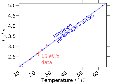
Figure 1: Hindman’s data (from [23]), for the longitudinal relaxation time, $T_{1,0}$, of water vs. temperature, $T$, at an NMR resonance frequency of 60  MHz, and the corresponding fit in blue (dark gray), accompanied by $T_{1,0}$ data that we measured at an NMR resonance frequency of 15 MHz at the sample conditions used throughout this paper in red (light gray). Since most applications of ODNP for the study of hydration dynamics will employ samples that are not deoxygenated, Hindman’s data has been adjusted by increasing the relaxation rate by $70\times 10^{-3}\;\mbox{s}^{-1}$ to account for the resulting additional relaxation mechanisms; the adjustment leads to a good match for the data we measured. (We denote the longitudinal relaxation time as $T_{1,0}$ to explicitly exclude the presence of spin probe).

This derivative maximum near ambient temperature makes the $T_{1,0}$ time of water an important intrinsic measurement of the sample temperature, which can track the changes in sample temperature with increasing microwave power. Obviously, the $T_{1,0}$ time will be most sensitive to temperature changes near ambient temperature. Furthermore, since the curvature (i.e. second derivative w.r.t. temperature) vanishes, the $T_{1,0}$ time also depends approximately linearly on temperature (fig. 1).

For standard measurements of the $T_{1}$ and $T_{1,0}$ times, we can fit the integrated signal intensities ($cM(\tau)$) from inversion recovery or saturation recovery experiments to the standard form

$$cM(\tau) =cM(\infty)+c\left(M(0)-M(\infty)\right)e^{-\tau/T_{1}},$$ (2)

where $\tau$ gives the magnetization recovery delay, $M(0)$ gives the initial magnetization in the recovery curve ($-M(\infty)$ for inversion recovery, 0 for saturation recovery), $M(\infty)$ gives the steady-state magnetization (i.e. after infinite recovery delay), and $c$ is a flexible fit parameter. Note that the “$T_{1}$” above could equally well be the $T_{1}$ of a sample with spin probe, or the $T_{1,0}$ of one without.

We will also require a method capable of measuring time-dependent variations in the $T_{1,0}$ time that occur on a timescale faster than $T_{1,0}$. By rapidly repeating saturation-recovery with a fixed recovery time, $\tau$, much shorter than $T_{1,0}$, we can repeat a train of acquisitions at a rate of two to three scans per $T_{1,0}$ period, and so avoid the recovery time of $5\times T_{1,0}$ between subsequent signal acquisitions required by inversion recovery measurements. Eq. 2 will still allow a relative comparison of $T_{1,0}$ times for the various acquisitions, even when $\tau$ is significantly small relative to $T_{1,0}$. Though intrinsically less accurate than an inversion recovery or saturation recovery experiment acquired over several recovery delay points, the faster experiment will allow us to determine – with about 1 s time resolution – how rapidly the sample temperature responds to changes in incident microwave power.

II.2 Source of the Microwave-Induced Heating Effect

The interaction between the electric field of the microwaves and the aqueous solution (which is a dielectric) induces changes in bulk water dynamics, which lead to the changes in relaxation time, $T_{1,0}$, that we measure. For convenience, our model will describe this change in dynamics simply as an increase in the temperature of the solution, i.e. as heating. However, before we consider the impact on the ODNP enhancements, we first examine the effects of the dielectric interaction. In particular, we note that – while sufficient within the scope of this article – a temperature-based description may provide only a limited insight into a more complex interaction.

Simply put, the electric field only induces specific modes of molecular motion. Excitation of a mode can contribute a mixture of adiabatic and irreversible changes to the molecular dynamics within the sample solution. Meanwhile, the air flowing around the capillary that contains the sample is actively removing heat from the system, even as heat is entering the system via the dielectric excitation. To the best of our knowledge, it has not been clarified whether or not one expects all modes of molecular motion to maintain a thermal equilibrium or not under such a setup.

We believe it is worthwhile to pause and clarify the effect of dielectric interactions in terms of the standard Debye model. Though, in this article, we will not quantitatively employ this equation, it helps us to classify the timescales and molecular motions associated with the dielectric interaction between the microwaves and the sample solution. Specifically, it gives a complex permittivity (i.e. complex dielectric coefficient), $\hat{\varepsilon}(\omega)$, that varies with the frequency, $\omega$, of the electric field of the radiation, namely,

$$\hat{\varepsilon}(\omega)= \varepsilon_{\infty}+\sum_{k}\frac{c_{k}}{1+i\omega\tau_{k}},$$ (3)

which is broken down in terms of $\varepsilon_{\infty}$ – the limiting dielectric permittivity at frequencies with periods far faster than the relevant relaxation times – and a sum over $k$ dielectric relaxation processes (i.e. mechanisms). The $\tau_{k}$ are the dielectric relaxation times associated with the various relaxation mechanisms, the $c_{k}$ are the coefficients describing the relative dominance of the different mechanisms, and $\omega$ is the angular frequency ($\left[\mbox{rad}/\mbox{s}\right]$) of the electric field of the radiation.

It is important to note that all dielectric interactions relevant for water at X-band (i.e. $\sim$10 GHz) frequencies necessarily involve changes to the molecular dynamics of the water. In pure water, there is only one mechanism that contributes significantly to the dielectric permittivity in the range of frequencies up to and including X-band microwaves (i.e. $\sim$10 GHz). The relevant molecular motions involve overall rotations of the water molecule about axes perpendicular to its electric dipole and require a finite relaxation time of $\tau_{k}=8.3\;\mbox{ps}$ [26]. Solutes introduced into the water can have various effects on this dielectric relaxation process: they may change the relaxation time, $\tau_{k}$, of the bulk water; they may inhibit the modes of motion that contribute to the 8.3 ps  process, leading to a decrease in the corresponding $c_{k}$ value; and/or – especially in the case of macromolecules – they may introduce new relaxation processes with slower relaxation times, thus introducing new terms to the sum over the $k$ dielectric relaxation mechanisms aside from the one corresponding to the 8.3 ps process [26, 27, 28].

By remembering that the microwave resonator (e.g. cavity) is simply an electric circuit, we come to better understand the meaning and relevance of the complex permittivity. A sample whose dielectric permittivity, $\hat{\varepsilon}(\omega)$, at the incident microwave frequency is entirely real-valued can sit in the electric field generated by the resonator without dissipating any power and therefore without generating any heat. Of course, the sample does change the capacitance (or, more generally, reactance) of the circuit because it cyclically stores and releases the energy of the applied electric field by changing the alignment of its molecular electric dipoles. The real part of the dielectric permittivity thus quantifies how much “reactive” or “adiabatic” molecular motion the electric field induces in the sample solution. By contrast, a sample with an imaginary-valued dielectric implies an increase in the effective resistance of the resonator, which in turn implies a conversion of microwave power into heat. Stated differently, the relative magnitude of the imaginary part gives the amount of incident radiation absorbed by the solution that is eventually dissipated as heat [29]. As this motion leads to a change in the heat in the system, unlike the molecular motion induced by the real part of the dielectric, we refer to it as “irreversible.”

The form of eq. 3 allows us to identify whether the contribution of a particular dielectric relaxation mechanism (i.e. $k$ term) is significant at a particular microwave frequency, and if so, whether the associated molecular motions cause adiabatic or irreversible changes to the molecular dynamics. Specifically, when the incident microwave frequency is much slower than the dielectric relaxation time ($\omega\ll 1/\tau_{k}$), $\hat{\varepsilon}$ is entirely real, corresponding to an adiabatic change in dynamics. At angular frequencies near $1/\tau_{k}$ the imaginary part of the $k^{th}$ mechanism (i.e. $\left|\Im\mathfrak{m}\left[c_{k}/1+i\omega\tau_{k}\right]\right|=c_{k}\omega\tau_{k}/1+\omega^{2}\tau_{k}^{2}$) rises to a broad maximum, which indicates irreversible changes in the dynamics. For example, for the primary relaxation process in bulk water at 8.3 ps [26], the water molecules will respond adiabatically to fields in the DC to low microwave regime. Over a broad range of frequencies near $1/2\pi\tau_{k}\approx 19\;\mbox{GHz}$, the sample absorbs microwaves, whose energy irreversibly drives the relatively disordered modes of motion associated with this relaxation process. Simultaneously, at these frequencies, the real component of the dielectric (i.e. $\Re\mathfrak{e}\left[c_{k}/1+i\omega\tau_{k}\right]=c_{k}/1+\omega^{2}\tau_{k}^{2}$) and adiabatic changes to the dynamics coming from that particular mode (i.e. the $k^{th}$ mode) fall to half their maximum amplitude, reaching zero at higher frequencies. Finally, at even higher frequencies ($\omega\gg 1/\tau_{k}$), the imaginary component and associated irreversibly driven motion associated with that particular mode become negligible as well.

Thus, the electric fields in the X-band regime will change the molecular dynamics of the solution in several ways that could potentially alter the NMR bulk relaxation time, $T_{1,0}$. In X-band ODNP experiments, we employ a microwave frequency of $\sim$10 GHz, which we expect will induce both adiabatic and irreversibly driven dipole reorientation in the bulk water. Each could potentially contribute to changes of the $T_{1,0}$ time. However, only the irreversibly driven dipole reorientation will change the actual sample temperature. Hydration water on bimolecular surfaces display slower modes of motion that may further complicate this picture. For instance, in a recent study of an aqueous solution of ribonuclease A at ambient temperature, Oleinikova et. al. present a dielectric relaxation time $\tau_{k}$ of 35 ps, which they assign to reorientation of the hydration water [28]. We expect the dielectric interaction to irreversibly drive some limited changes to the molecular dynamics of such hydration water. The extent to which these changes impact the translational hydration water dynamics, as measured by ODNP, as well as the rate of molecular exchange and heat transfer between the hydration water and the bulk water could both provide interesting information, but remain relatively undetermined.

This understanding provides an important background for the way we use the word “temperature” in this article. If we were to compare one sample that is irradiated by microwaves at $\sim$10 GHz, while simultaneously actively cooled by air flowing around the sample capillary tube (like in our experimental setup), to another sample of identical composition that is not irradiated but, rather, simply heated until it yields the same $T_{1,0}$ as the first sample, then we must concede that the molecular dynamics of the two samples may not match. Similarly, it is not trivial to determine what, if any, effect the adiabatically driven motion will have on the $T_{1,0}$ rate. All these complications could lead to a richer interpretation of the heating effect that may validate future studies. In particular, as previously explained (eq. 1), the value of $T_{1,0}$ depends primarily on proton-proton dipolar coupling, which lends one to believe that it would be more sensitive to the rotations of water molecules induced by the dielectric interaction. In fact, the temperature dependence of $T_{1,0}$ has even been shown to closely follow that of the rotational motion of the individual water molecules, as – for instance – observed by ¹⁷O NMR [23]. This fact, in combination with the previously mentioned complications lends interesting motivations to direct future publications towards investigating the observation (presented later) that the relaxivities $k_{\rho}$ and $k_{\sigma}$, which encode the information about the local dynamics of water near the spin probe, remain relatively constant with microwave power, despite relatively dramatic changes in $T_{1,0}$.

Setting these interesting possibilities aside, however, throughout this article we employ the definition of effective “temperature” to be the equilibrium temperature at which the $T_{1,0}$ is elevated to the same value that we observe under steady-state dielectric excitation. This is the definition most relevant to the changes in the ODNP measurements that we observe.

II.3 Impact of Heating on ODNP

Through changes in the $T_{1,0}$ time, increases in the effective temperature drive increases in the steady-state ODNP enhancement, as well as increases in the repetition delay necessary between each NMR acquisition. After reviewing the extant theory, which is derived predominantly from Hausser and Stehlik [8], we first explain how lengthened NMR relaxation times at high power can lead to artifacts in the ODNP enhancement vs. power, i.e. $E(p)$, data. Then we outline how the lengthened $T_{1,0}$ time leads to unexpectedly high values for the actual enhancement. Finally, we present a new strategy for data analysis that both compensates for these changes in $T_{1,0}$ and allows determination of the hydration dynamics at tens of micromolar concentrations.

II.3.1 Review of Previous Theory

For clarity, we note that while previous work by Han et. al. [1, 6, 2, 4, 30, 15] has denoted the coupling factor with $\rho$, here we will use $\xi$ for the coupling factor, since (consistently with other literature [10, 8, 31, 32]) we reserve $\rho$ for the local self-relaxation rate (table 2).

The polarization transferred from the electron spin to the protons is inverted relative to the thermal polarization of the protons. Thus, sufficient amounts of polarization transfer lead to enhanced and inverted NMR signal. The enhancement, $E$, is defined as the ratio between the ODNP-enhanced proton signal and the thermal signal. We also find it convenient to refer to the amount of “polarization transferred,” $1-E$. As shown by Hausser and Stehlik [8], the amount of polarization transferred can be broken down into a product,

$$1-E(p)=\xi s(p)f\left|\frac{\omega_{e}}{\omega_{H}}\right|,$$ (4)

where the coupling factor, $\xi$, the leakage factor, $f$, and the saturation factor, $s$, all affect the efficiency with which electron spin polarization, whose equilibrium population is approximately proportional to the ESR resonance frequency $\omega_{e}$, transfers to the inverted nuclear spin polarization, whose equilibrium population is approximately proportional to the proton Larmor frequency $\omega_{H}$. For nitroxide spin probes in aqueous solution, we have measured the ratio of $\omega_{e}$ to $\omega_{H}$ as 659.32. To extract the information pertaining to local hydration dynamics, we wish to accurately isolate the coupling factor, $\xi$, from the other parameters.

The leakage factor, $f$, gives the proportion of the total proton relaxation that is due to the local dipolar relaxation mechanisms

$$f=\frac{\rho}{\rho+T_{1,0}^{-1}}$$ (5)

Since the total longitudinal relaxation rate of a solution containing a spin probe, $T_{1}^{-1}$, is the sum of the bulk, $T_{1,0}^{-1}$, and the local dipolar relaxation rate, $\rho$, i.e.

$$T_{1}^{-1}=\rho+T_{1,0}^{-1},$$ (6)

one typically writes the leakage factor as

$$f=1-\frac{T_{1}}{T_{1,0}.},$$ (7)

since inversion recovery experiments can directly determine both $T_{1}$ and $T_{1,0}$.

The saturation factor, $s(p)$, gives the net saturation of all electron spins in the sample. In the absence of microwave power, $s=0$, while in the limit of microwave power, it approaches a value of $s_{max}$. For ¹⁴N nitroxides, $\frac{1}{3}\leq s_{max}\leq 1$, as discussed below. Standard ESR theory [33], as well as its specific application to ODNP [6, 7] indicates that (for well separated Lorentzian absorption lines), the saturation factor follows an asymptotic form

$$s(p)= \frac{s_{max}p}{p_{1/2}+p}.$$ (8)

Here, $p_{1/2}$ is the power needed to achieve half of the maximum possible saturation. For clarity, we can substitute this into eq. 4, yielding

$$1-E(p)=\xi f\left|\frac{\omega_{e}}{\omega_{H}}\right|\frac{s_{max}p}{p_{1/2}+p}.$$ (9)

A variety of factors, including the electron spin relaxation time and the electrical properties of the resonant cavity combine to determine the value of $p_{1/2}$. Therefore, the previously employed analysis extrapolates the enhancements to their asymptotic limit

$$\lim_{p\rightarrow\infty}E\equiv E_{max},$$ (10)

thus eliminating the dependence on $$p_{1/2}$$ to give (via 4 and 8)

$$1-E_{max}= \xi s_{max}f\left|\frac{\omega_{e}}{\omega_{H}}\right|.$$ (11)

Later, for reasons that will become obvious, we will refer to eq. 9-11 (where $f$ is assumed a constant) as the “uncorrected model” when it is employed to experimentally determine the coupling factor.

To determine $\xi$ from 11, one must still determine the value of $s_{max}$. Previously, Armstrong and Han [6] presented the most complete analysis describing the key mechanisms behind total electron spin saturation (i.e. the net contribution from all ESR lines). Their analysis is relevant for quantifying the ODNP effect for both freely dissolved spin probes and those tethered to larger molecular systems, as it describes the effects of both Heisenberg exchange and nitrogen spin relaxation on the three (or two) hyperfine states of ¹⁴N (or ¹⁵N) of stable nitroxide spin probes in order to predict $s_{max}$ as a function of free nitroxide spin probe concentration and nitrogen nuclear spin relaxation. Notably, they predict that for biological or polymer samples with covalently tethered spin probes, $s_{max}$ should closely approach 1 [6].

	Previous Notation of Han et. al.		Standard Notation
self-relaxation rate	$kC$	$\Rightarrow$	$\rho$
coupling factor	$\rho$	$\Rightarrow$	$\xi$

Table 1: For those more familiar with notation previously used by Han et al., this table translates to the standard notation.

	Standard Symbol	Relaxivities	Transition Rates
local dipolar self-relaxation rate	$\rho$	$k_{\rho}C$	$w_{0}+2w_{1}+w_{2}$
local dipolar cross-relaxation rate	$\sigma$	$k_{\sigma}C$	$w_{2}-w_{0}$
coupling factor	$\xi$	$\displaystyle\frac{k_{\sigma}}{k_{\rho}}$	$\displaystyle\frac{w_{2}-w_{0}}{w_{0}+2w_{1}+w_{2}}$
leakage factor	$f$	$\displaystyle\frac{k_{\rho}C}{k_{\rho}C+T_{1,0}^{-1}}$	$\displaystyle\frac{w_{0}+2w_{1}+w_{2}}{w_{0}+2w_{1}+w_{2}+w^{0}}$
nuclear longitudinal relaxation rate	$T_{1}^{-1}$	$k_{\rho}C+T_{1,0}^{-1}$	$w_{0}+2w_{1}+w_{2}+w^{0}$

Table 2: Each column summarizes an equivalent means for denoting a quantity: the terminology for the parameter, the symbol used in the standard notation, and equivalent expressions in terms of both the concentration-independent relaxivities and the transition rates, respectively. Wherever possible, all notation matches that of Solomon [19] and Hausser [8]. This work, which explores various concentration-dependent effects, makes frequent use of the concentration-independent relaxivities (even though the $k_{\rho}$, $k_{\sigma}$ notation is not used elsewhere). Furthermore, since $k_{\rho}$ and $k_{\sigma}$ explicitly denote relaxation processes localized (i.e. $\propto r^{-6}$) around the spin probe, they provide interesting information about the hydration dynamics, which is complementary to information derived from the coupling factor, $\xi$ (compare, for instance to [3, 34]). This publication does not make use of the transition rate notation [8, 19], but it is provided here in the third column for comparison.

In summary, the previous (i.e. uncorrected) analysis advises one to determine the enhancement at several values of microwave power and to extrapolate to an asymptotic limit of the signal enhancements, $E_{max}$, as a function of microwave power. The value of $E_{max}$ is then inserted into eq. 11. By employing inversion recovery experiments with and without spin probe to obtain (respectively) $T_{1}$ and $T_{1,0}$ as inputs for eq. 7, one could obtain a value for the leakage factor ($f$) needed for eq. 11. Finally, one can determine the value for $s_{max}$ in eq. 11 through one of several means: from a concentration series [6, 7], from calculations based on the known exchanges rates for small freely dissolved spin probes determined by Bennati et. al. [11], or from the reasonable approximation that $s_{max}\approx 1$ for most macromolecular (e.g. proteins, polymers, vesicles) samples with tethered spin probes. Researchers have employed the uncorrected analysis (eq. 11) fairly routinely to extract $\xi$. By way of the translational correlation time, $\tau_{c}$, given by the force free hard sphere model of relaxation [35], the value of $\xi$ can in turn determine the local translational diffusivity, $D_{local}$, of the biological water coupled to protein or soft matter surfaces or embedded in their interiors. (Detailed equations for the calculation of both $s_{max}$ and $D_{local}$ are reviewed at the end of the theory section.) With a series of differently positioned spin probes, one can map out the hydration dynamics at different sites of the macromolecule [1, 3, 36, 37, 4, 5, Kausik2009a, 30].

However, the analysis and experiment (i.e. eq. 11) previously employed in these and other investigations expects only the saturation factor, $s(p)$, to vary with microwave power, $p$, and does not account for the fact that both the $T_{1}$ time of the spin labeled sample – which is important for setting experimental parameters – as well as the leakage factor, $f$, vary with microwave power, as laid out in this work. Both these variations come predominantly from an underlying change in the $T_{1,0}$ time as the microwave power increases

$$T_{1,0}(p)\approx T_{1,0}(0)+p\left.\frac{\partial T_{1,0}}{\partial p}\right|_{p=0}.$$ (12)

We denote this more compactly as

$$T_{1,0}(p)\approx T_{1,0}+p\Delta T_{1,0},$$ (13)

where the parameter $T_{1,0}\equiv T_{1,0}(0)$ quantifies the bulk relaxation time in the absence of microwave irradiation, while the new parameter $\Delta T_{1,0}$ quantifies the variation of the bulk relaxation with incident microwave power. For the aqueous solution of free nitroxide spin probes studied here, $T_{1,0}(p)$ is exactly the relaxation time of pure water, which depends linearly on temperature, as discussed earlier. Since both the heat capacity and the dielectric absorption coefficient (and therefore the conversion of microwave power into temperature) of water should remain relatively constant near ambient temperature, we can anticipate that eq. 13 is a very good approximation. Indeed, we have experimentally verified that $T_{1,0}(p)$ remains linear with power (as will be shown in fig. 6). One easily could, but typically will not need to, include any higher order terms, such as $p^{2}\Delta^{2}T_{1,0}$.

II.3.2 Experimental Considerations

In the past, researchers set the repetition delay between NMR signal acquisitions by assuming that the $T_{1}$ of a sample remained constant, whether or not it was irradiated with microwaves. They either acquired signal at $5\times$ to $10\times T_{1}$ or acquired ODNP data with a fast repetition time ($\approx 0.5\;\mbox{s}$) in an Ernst angle experiment. We will demonstrate that, even though they represent the standard for most NMR experiments, the fast repetition experiments lead to large discrepancies in ODNP measurements. Specifically, because heating increases the bulk water relaxation time $T_{1,0}$, it selectively suppresses the amount of signal detected at high microwave powers ($p\gg T_{1,0}/\Delta T_{1,0}$), as shown below. Because this causes the $T_{1}$ of low concentration samples to lengthen considerably with even relatively small amounts of sample heating, this effect can easily lead to erroneous or inconsistent measurements of the enhancements; however, with appropriate consideration, this situation is easily avoided.

We now analyze this signal suppression in detail. As previously discussed, an ODNP experiment involves several scans that determine the enhancements at a series of different microwave powers, $E(p)$. Each scan generally consists of a train of resonant rf pulses of a constant flip angle, $\theta$, separated by a constant repetition delay, $t_{r}$. For instance, the optimized Ernst-angle experiment employs an angle such that $\cos(\theta)=\exp\left(-t_{r}/T_{1}\right)$. For a steady-state pulse train, the Bloch equations determine the fraction of available magnetization that the NMR relaxation between scans actually manages to recover; this is [38]

$$\frac{M_{pt}}{M_{\infty}}= \frac{1-\exp\left(-\displaystyle\frac{t_{r}}{T_{1}}\right)}{1-\cos(\theta)\exp\left(-\displaystyle\frac{t_{r}}{T_{1}}\right)}\sin(\theta).$$ (14)

Here, $M_{pt}$ gives the fraction of the ODNP-enhanced magnetization that the pulse train actually detects, while $M_{\infty}$ gives the total ODNP-enhanced magnetization in the absence of any pulses.

In order to explore how the change in $T_{1,0}$ with power affects samples of different spin probe concentrations differently we find it useful to explicitly denote the concentration, $C$, by making use of the self-relaxivity constant, $k_{\rho}$,

$$k_{\rho}=\frac{\rho}{C}$$ (15)

(table 2). From eq. 6 (the relationship between $T_{1}$ and $T_{1,0}$), and eq. 13 (the power dependence of $T_{1,0}$), we then retrieve the longitudinal relaxation for a given spin probe and hardware setup rate as a function of concentration and microwave power

$$T_{1}^{-1}(p)= k_{\rho}C+T_{1,0}^{-1}(p)$$

$$= k_{\rho}C+\left(T_{1,0}+p\Delta T_{1,0}\right)^{-1}.$$ (16)

We can measure or estimate $\Delta T_{1,0}$ for a specific hardware setup and type of sample composition, and we can also roughly estimate the relaxivity, $k_{\rho}$. Substitution of this value into eq. 14, directly leads to the amount of signal suppression as a function of microwave power,

$$\frac{M_{pt}}{M_{\infty}}= \frac{\sin(\theta)\left(1-\exp{\left(-t_{r}k_{\rho}C-t_{r}\left(T_{1,0}+p\Delta T_{1,0}\right)^{-1}\right)}\right)}{1-\cos(\theta)\exp{\left(-t_{r}k_{\rho}C-t_{r}\left(T_{1,0}+p\Delta T_{1,0}\right)^{-1}\right)}}.$$ (17)

At high spin probe concentration, the power dependence remains minimal (since the $t_{r}k_{\rho}C$ term dominates), leading to equal signal suppression at all microwave powers. Therefore, for instance, acquisition with a fast repetition delay at high concentrations gives accurate and reproducible data. However, at low spin probe concentrations, the power-dependent term arising from the bulk relaxation (the second term inside the exponential in eq. 17) becomes more significant; therefore, the signal suppression ($M_{pt}/M_{\infty}$) varies with microwave power, as previously mentioned. Such an experiment will not record the actual ODNP enhancement, $E$, but rather, an apparent enhancement, $EM_{pt}/M_{\infty}$. Because the signal suppression of eq. 17 obscures the true enhancement, we refer to it as an artifact.

To routinely avoid this artifact in the data, we simply employ eq. 16 to predict the longest $T_{1}$ that occurs during the ODNP experiment

$$T_{1,max}= \frac{T_{1,0}+p_{max}\Delta T_{1,0}}{k_{\rho}C\left(T_{1,0}+p_{max}\Delta T_{1,0}\right)+1},$$ (18)

which occurs for the ODNP scan that employs the maximum microwave power $p_{max}$. Again, we remind the reader that all the parameters above are either known or can be estimated. By employing a repetition time of at least $5\times T_{1,max}$, we can insure that the signal for each scan quantitatively includes all ODNP-enhanced magnetization, thus preventing artifacts. Of course, to acquire reproducible data, one must always measure the actual value of $T_{1,max}$ for a sample; this is not troublesome, since the same value is required for the correction described in the following section.

II.3.3 Impact of Heating on ODNP Enhancements

Now that the preceding section explains how to detect the actual enhancements, $E$, we can determine the effect of sample heating on the actual enhancements. Specifically, we examine how the change in bulk water relaxation impacts the leakage factor, and therefore (via. eq. 9) the enhancements. One can combine eqs. 5,13, and 15 to quantify how the leakage factor, $f$, varies with microwave power, p, and concentration, C:

$$f(p,C)= \frac{k_{\rho}CT_{1,0}\left(1+p\frac{\Delta T_{1,0}}{T_{1,0}}\right)}{1+k_{\rho}CT_{1,0}\left(1+p\Delta\frac{T_{1,0}}{T_{1,0}}\right)}.$$ (19)

Note that though the relaxivity, $k_{\rho}$, and thus the local water dynamics around the spin probes, does vary somewhat with temperature [12], we will find (in the results section) that for samples with concentrations of spin probe on the order of hundreds of micromolar or less (i.e. typically desirable concentrations for biological samples), the change in $p\Delta T_{1,0}$ overwhelms any variation due to changes in $k_{\rho}$.

Let us examine eq. 19 in the limiting extremes of spin probe concentration, $C$. At high concentration, where the relaxation of the water protons near the spin probe dominates over the relaxation of the water protons in the bulk (i.e. $Ck_{\rho}T_{1,0}\gg 1$), $f(p)$ has a value close to 1 and changes little with power. On the other hand, at low concentration (i.e. $Ck_{\rho}T_{1,0}\ll 1$), the denominator approaches 1 and $f(p)$ varies linearly with power.

If one applies the uncorrected analysis (eq. 11) to enhancement data taken from low concentration samples, the change in the leakage factor with power expressed by eq. 19 will obscure the true value of the coupling factor, $\xi$. From the expressions for $f(p,C)$ (eq. 19) and $1-E(p)$ (eq. 4), we can determine the effect of the changing leakage factor on the enhancements. We take the ratio of the amount of polarization transferred ($1-E(p)$) in the presence and absence of microwave heating that changes the bulk relaxation time. In other words, we can determine the ratio of the value expected by the uncorrected model to the actual value that we expect, including heating effects:

$$\frac{1-E_{\mbox{\scriptsize heating}}(p)}{1-E_{\mbox{\scriptsize no heating}}(p)} =\frac{f(p)}{f(0)}\quad\quad\quad\quad$$

$$=\frac{1+k_{\rho}CT_{1,0}}{1+k_{\rho}CT_{1,0}\left(1+p\frac{\Delta T_{1,0}}{T_{1,0}}\right)}\left(1+p\frac{\Delta T_{1,0}}{T_{1,0}}\right)$$ (20)

As long as the fractional change in the bulk water relaxation, $p\Delta T_{1,0}/T_{1,0}$, remains small enough, this “drift” in the net polarization transferred remains roughly linear with microwave power. We expect (and will see) that the drift in the leakage factor, $f$, leads to a linear variation of the enhancements in the high power regime (eq. 20), while the previous theory (eq. 11) expects the enhancements to approach their asymptotic maximum and, therefore, remain constant. This drift causes problems when attempting to reproducibly extrapolate the enhancements to the asymptotic maximum, $E_{max}$, as required by the uncorrected analysis. Not only will it prevent data from fitting the model perfectly, but also, even slight changes to the characteristics of the hardware can lead to changes in $\Delta T_{1,0}$; furthermore, changes to the range and spacing of the microwave powers, $p$, sampled by the experiment will lead to different weighting of data points with different leakage factors (eq. 20). Therefore, any attempt to extrapolate to the asymptotic maximum, $E_{max}$, will necessarily give varying results. As a result, for samples with nitroxide probe concentrations below about 1 mM ($\approx 1/k_{\rho}T_{1,0}$ for bulk water), the uncorrected analysis (eq. 11) only gives approximate values for the coupling factor, $\xi$. Still, the uncorrected analysis can accurately identify meaningful changes in the coupling factor ($\xi$) value and thus identify changes or trends in the translational hydration dynamics for similar samples. However, the reproducibly of such measurements critically depends on the exact duplication of both the experimental and hardware parameters for all the $\xi$ values that are being compared.

II.3.4 The Corrected Analysis

Having reviewed the relevant parts of the existing ODNP theory and pointed out its limitations, we now seek to increase the accuracy with which we extract the dynamic parameter $\xi$ from the enhancement values. We seek a new approach to data acquisition and analysis that can correct for those errors that arise as a result of dielectric absorption and heating (i.e. eq. 20). At the same time, we seek a method that can extract meaningful information about the hydration dynamics at low concentrations, where the leakage factor ($f$) (determined in eq. 7 and used in eq. 11) approaches zero, and thus would appear to make the coupling factor ($\xi$) ill-determined.

The equation that gives the enhancements (eq. 4) has historically been phrased in terms of the unitless leakage factor, $f$, and the unitless coupling factor, $\xi$. As we can already see from the complexity of eq. 20, this strategy poses a problem when attempting to analyze concentration-dependent effects such as dielectric heating. However, Hausser and Stehlik [8] derive $f$ and $\xi$ from three more fundamental rates: the rate of local dipolar cross-relaxation between the electron and the proton, $\sigma$, the local dipolar self-relaxation rate of the protons, $\rho$, and the intrinsic relaxation rate of the bulk water protons, $T_{1,0}^{-1}$ (all of which have units s^-1), which includes any relaxation driven by mechanisms that do not involve the spin probe. To these parameters, we add $\Delta T_{1,0}$, which is determined by the particular hardware configuration.

We note that the $T_{1,0}$ time depends only on the characteristics of the unlabeled solution. By contrast, $\sigma$ and $\rho$ come from interactions that scale with distance, $r$, from the spin label as $r^{-6}$. Thus, they depend only on the local water dynamics in the sample under investigation, and scale with spin label concentration. Therefore, rather than referring to $\rho$ and $\sigma$, we can refer to the self-relaxivity, $k_{\rho}$, defined earlier (eq. 15) and the similarly defined cross-relaxivity

$$k_{\sigma}=\frac{\sigma}{C}.$$ (21)

These relaxivity parameters have units $\mbox{s}^{-1}\mbox{M}^{-1}$ (table 2).

The corrected analysis now separately determines $k_{\sigma}$ (from the measurements of $E(p)$ and $T1(p)$) and $k_{\rho}$ (from the measurements of $T_{1,0}$ and $T_{1}$), as will be detailed below. While the values $E_{max}$ and $f$ of the uncorrected analysis (eq. 11) are both dependent on – but not linearly proportional to – the spin probe concentration, the bulk water relaxation rate, $T_{1,0}^{-1}$, and a heating-induced term of the form $p\Delta T_{1,0}$ (from eq. 13), the values of $k_{\sigma}$ and $k_{\rho}$ depend on neither the spin probe concentration, nor $T_{1,0}^{-1}$, nor $\Delta T_{1,0}$. As we will demonstrate, this allows one to bypass the heating effects and to determine meaningful information at low concentration. The ratio of these two local relaxivities

$$\xi=\frac{k_{\sigma}}{k_{\rho}},$$ (22)

gives the unitless coupling factor, and thus information about the translational correlation time $\tau_{c}$, which translates to a unique value for the local translational diffusivity, $D_{local}$.

We now outline the specifics of the analysis described above, which consists of the following steps:

1. Interpolate a small set of measurements of $T_{1}(p)$ to generate values corresponding to all microwave powers at which we measure the ODNP signal enhancements, $E(p)$.

2. Determine a set of $k_{\sigma}s(p)$ values at all microwave powers, $p$.

3. Find the asymptotic limit, $k_{\sigma}s_{max}$.

4. Determine $k_{\sigma}$.

5. Perform $T_{1}$ measurements in the absence of microwave power, on both the spin labeled sample and an unlabeled reference sample, in order to determine $k_{\rho}$.

6. Determine $\xi=k_{\sigma}/k_{\rho}$ which in turn yields the $\tau_{c}\propto\left(D_{I}+D_{SL}\right)^{-1}$ value.

Step 1

In order to quantify the $k_{\sigma}s_{max}$ values to ultimately determine $k_{\sigma}$, one must first determine $T_{1}(p)$ values for each $E(p)$ data point. Specifically, these values will be employed in step 2 to correct for heating effects. Typically, one does not have the experimental time to measure the $T_{1}(p)$ at all microwave powers ($p$), and so we need a method for interpolating the relatively few $T_{1}(p)$ values we measure to reasonably predict $T_{1}(p)$ at all microwave powers. From eq. 16, we recall the NMR $T_{1}$ rate in the absence of microwaves:

$$T_{1}^{-1}(0)=k_{\rho}C+T_{1,0}^{-1}$$

as well as the rate we expect when microwave power is applied (i.e. eq. 16 identically):

$$T_{1}^{-1}(p)=k_{\rho}C+\left(T_{1,0}+p\Delta T_{1,0}\right)^{-1}.$$ (23)

Subtraction of these two equations, followed by some rearrangement leads to the value

$$F_{linear}(p)\equiv\frac{1}{T_{1}^{-1}(p)-k_{\rho}C}\approx T_{1,0}+p\Delta T_{1,0}.$$ (24)

We can determine $k_{\rho}C$ from the $T_{1}$ data with power off (eq. II.3.4), namely

$$k_{\rho}C=T_{1}^{-1}(0)-T_{1,0}^{-1}.$$ (25)

As noted in eq. 24, $F_{linear}$ is an approximately linear function of microwave power. Thus, by fitting the values of $F_{linear}(p)$ to a straight line, then solving for

$$T_{1}(p)=\frac{1}{F_{linear}^{-1}(p)+k_{\rho}C}$$ (26)

one can retrieve an accurately interpolated value for $T_{1}(p)$.

We make two practical notes at this point: First, a thresholding procedure at high concentration where $T_{1}(p)^{-1}\approx k_{\rho}C$ is required to manually set $T_{1}(p)$ to $k_{\rho}C$ in order to prevent numerical blow-up of $F_{linear}$. Second, this interpolation procedure can be performed without the need for a $T_{1,0}$ measurement. Eq. 24 and eq. 26 do not depend very sensitively on the value of $T_{1,0}$. A reasonable first estimate of $T_{1,0}$ will usually suffice, and when it does not, one can determine $T_{1}(p)$ from a very closely spaced interpolation.

Step 2

With the help of eq. 22, 5, and 15, we rewrite the previous equation for the signal enhancements (eq. 4) in terms of the fundamental relaxivities

$$1-E(p)=\overbrace{\frac{k_{\sigma}}{k_{\rho}}}^{\mbox{\small$\xi$}}\overbrace{\frac{k_{\rho}C}{k_{\rho}C+T_{1,0}^{-1}(p)}}^{\mbox{\small$f$}}\left|\frac{\omega_{e}}{\omega_{H}}\right|s(p).$$ (27)

We can now multiply by the form of $T_{1}(p)$ given by eq. 16 ($T_{1}(p)=1/(k_{\rho}C+T_{1,0}^{-1}(p))$), then cancel and rearrange terms to arrive at

$$k_{\sigma}s(p)=\frac{1-E(p)}{CT_{1}(p)}\left|\frac{\omega_{H}}{\omega_{e}}\right|.$$ (28)

Note that this is mathematically equivalent to the typical equation for the enhancements, eq. 4. However, it clearly illustrates how the variation of the $T_{1}(p)$ time with microwave power, as given by eq. 23 (i.e. eq. 16), perturbs the DNP signal enhancements. By inserting a value of $T_{1}(p)$ that is experimentally measured at (or interpolated to) the correct microwave power, one can fully account for the change in $T_{1,0}(p)$ that arises from dielectric heating. Inserting the interpolated $T_{1}(p)$ values from step 1 into eq. 28 should yield $k_{\sigma}s(p)$ values that depend asymptotically on power

$$\frac{1-E(p)}{CT_{1}(p)}\left|\frac{\omega_{H}}{\omega_{e}}\right| = k_{\sigma}s(p)$$ (29)

$$= \frac{k_{\sigma}s_{max}p}{p_{1/2}+p}$$

(where we have substituted eq. 8), in spite of mismatch of the enhancements, $E(p)$, to the uncorrected model (i.e. eq. 4,11). Thus, one can then proceed to extract accurate values of $k_{\sigma}s_{max}$ in spite of the drift in the enhancements at high microwave powers that we previously noted in eq. 20.

Step 3

Extrapolating eq. 29 to infinite power then yields $k_{\sigma}s_{max}$ in the same fashion that the uncorrected analysis extrapolated the signal enhancements to infinite power to find $E_{max}$, i.e.

$$k_{\sigma}s_{smax}=\lim_{p\rightarrow\infty}\left(\frac{1-E(p)}{CT_{1}(p)}\left|\frac{\omega_{H}}{\omega_{e}}\right|\right).$$ (30)

Note that the previously employed, uncorrected, analysis employs measurements of both $f$ or $\xi$. In order to determine either of these values, one must perform measurements on two samples: both the spin-labeled sample and the sample where the spin probe has been removed. Therefore, sample preparation issues with either sample can lead to errors in the measurement, as can discrepancies between the two samples. By contrast, note how one can determine $k_{\sigma}$ from measurements on only the spin-labeled sample.

Step 4

As with the uncorrected model, Armstrong’s model [6] then predicts a value for $s_{max}\approx 1$ for most spin labeled biological or soft matter samples, giving $k_{\sigma}\approx k_{\sigma}s_{max}$ directly. In the case of samples with freely dissolved spin label, as employed in Bennati et. al. [11], we can neglect the effect of nitrogen relaxation. We can then calculate the value of

$$s_{max}=1-\frac{2}{3+3b^{\prime\prime}}$$ (31)

for ${}^{14}N$ nitroxides where, following the work of Hyde and Freed [9], $b^{\prime\prime}=w_{h}/6w_{e}$ gives a ratio between the rate of Heisenberg exchange, $w_{h}$, and the rate of electron relaxation, $w_{e}$. ELDOR (electron double resonance) curves that measure both numbers on ¹⁵N nitroxides are presented by Bennati et. al. in [11] and lead to a value of $b^{\prime\prime}=C\times 198.7\;\mbox{M}^{-1}$, where $C$ is the spin label concentration.

Step 5

By referencing the relaxation time of the spin labeled sample to that of the unlabeled sample, we can determine $k_{\rho}$. Specifically,

$$k_{\rho}=\frac{T_{1}^{-1}-T_{1,0}^{-1}}{C}.$$ (32)

We determine $k_{\rho}$ entirely from measurements in the absence of microwave power, so that, as can be seen from eq. 23, dielectric heating effects are not an issue. It is also clear from eq. 32 that the determination of $k_{\rho}$ (as well as $k_{\sigma}$ cf. eq. 30) requires an accurate knowledge of the spin label concentration, $C$. One can often determine accurate concentrations of both spin labeled and non spin labeled biomolecules via UV-visible spectrophotometry or determine accurate concentrations of spin labeled biomolecules via ESR. However, as will be discussed in the next step, the accurate determination of the coupling factor – the ultimate parameter of interest – again does not require knowledge of the absolute concentration.

Step 6

Finally, we find the ratio of the two relaxivities (i.e. $k_{\sigma}$ and $k_{\rho}$) to give the coupling factor, $\xi$ (i.e. eq. 22), and – by extension – the local translational diffusivity of the hydration water. Up to this point, it is true that the individually determined relaxivities are susceptible to systematic errors in the actual concentration of spin probe, $C$, relative to the nominal concentration of the spin probe (see expressions for the relaxivities in $k_{\sigma}$ cf. eq. 30). However, issues with solubility, dilution, etc. can scale the concentration in both the labeled and unlabeled sample. During calculation and application of the leakage factor, $f$, in the previous analysis, such errors could be factored out, as long as samples were prepared in the same way. This final step of the newly proposed analysis also cancels such systematic errors, i.e. $\xi=(k_{\sigma}\cancel{C})/(k_{\rho}\cancel{C})$, (eq.22) in the same fashion.

The local translational diffusion coefficients can then be determined from

$$D_{local}\approx\left(D_{H_{2}O}+D_{SL}\right)\left(\frac{\tau_{c,bulk}}{\tau_{c,site}}\right).$$ (33)

Here, $D_{SL}=4.1\times 10^{-10}~{}\mbox{m${}^{2}$s${}^{-1}$}$ (the approximate diffusivity of small TEMPO derivatives) and $D_{\mbox{H${}_{2}$0}}=2.3\times 10^{-9}~{}\mbox{m${}^{2}$s${}^{-1}$}$ [1]. Each $\tau_{c}$ is the translational correlation time of a spectral density function that predicts the observed coupling factor ($\xi_{bulk}$ or $\xi_{site}$). Physically, this correlation time can be described as the lifetime of the dipolar interaction between the electron spin of the spin probe and the proton spin of the water molecule. We note that the “translational correlation time” is not necessarily a uniquely defined property of the molecular dynamics of a particular system. Rather, its exact value will also depend on the nature of the interaction probed by a particular measurement. Thus, we can expect that, even though they should exhibit similar trends and relative values, the translational correlation times generated by dynamics stokes shift spectroscopy [39], ODNP, as well as various scattering measurements might well be different from each other, even for systems with the same dynamics. By analogy, the rotational correlation time differs for different measurements, depending on whether the measurement probes the relaxation of an interaction that depends on rank one spherical harmonics (e.g. dielectric spectroscopy) or rank two spherical harmonics (e.g. NMR quadrupolar relaxation) [40, 41, 23, 28]. This highlights the usefulness of translating this number (even approximately) to a local translational diffusion, $D_{local}$, which is uniquely defined based solely on the local molecular dynamics; this is precisely the role of eq. 33.

The coupling factor, $\xi_{bulk}$, corresponding to the correlation time of unrestricted water, $\tau_{c,bulk}$, comes from the analysis of samples of small, freely dissolved spin-probes; in the results section, we will confirm a result of $\xi_{bulk}=0.33$. The value of the coupling factor is specific to the approximate static field, $B_{0}$, employed in the ODNP experiment. Following previous literature [12, 10, 6, 1, 3, 34] we employ Hwang and Freed’s expression for the spectral density function of the dipolar interaction between the spin probe and the water. This expression derives from a force free hard sphere (FFHS) model of translational diffusion and is proportional to

$$J(z)=\Re\mathfrak{e}\left[\frac{1+\frac{z}{4}}{1+z+\frac{4z^{2}}{9}+\frac{z^{3}}{9}}\right]$$ (34)

for which

$$z=\sqrt{i\omega\tau_{c}}$$ (35)

and it determines the functional form of the spectral density function,

$$\xi(B_{0},\tau_{c})=$$ (36)

$$\quad\frac{6J\left((\gamma_{e}-\gamma_{H})B_{0}\tau_{c}\right)-J\left((\gamma_{e}+\gamma_{H})B_{0}\tau_{c}\right)}{6J\left((\gamma_{e}-\gamma_{H})B_{0}\tau_{c}\right)+3J\left(\gamma_{H}B_{0}\tau_{c}\right)+J\left((\gamma_{e}+\gamma_{H})B_{0}\tau_{c}\right)},$$

where $\gamma_{e}=g\mu_{B}/h$ and $\gamma_{H}$ are the gyromagnetic ratios for the electron and proton spin, respectively. In order to generate this coupling factor, $\xi_{bulk}$, of 0.33 at a static field ($B_{0}=\omega_{H}/\gamma_{H}$) corresponding to the experimental NMR resonance frequency of $\omega_{H}/2\pi=14.8\;\mbox{MHz}$ we must choose an FFHS spectral density function with $\tau_{c,bulk}=33.3\;\mbox{ps}$. Note that eq. 33-II.3.4 apply equally well to the coupling factor determined either from the corrected analysis, as presented here, or from a coupling factor that the previously employed, uncorrected, analysis determines from leakage factor, $f$, and asymptotic enhancement, $E_{max}$ values.

III Results

III.1 Heating Artifacts

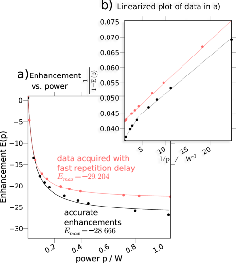
Figure 2: Fast repetition delays can generate a misleading artifact that alters the apparent enhancement as a function of microwave power. This artifact (here the difference between the red (gray) and black curves) can vary depending on the experimental setup and the exact value chosen for the repetition delay. It also obscures the underlying physics at work. We present data acquired with a 0.5 s repetition delay whose parameters and results (in red (gray)) match the parameters and results in [6]. An initial analysis would lead one to interpret the fact that the apparent enhancements (see eq. 17), $EM_{pt}/M_{\infty}$ – shown in red (gray), level off at high microwave powers (here, at powers higher than 0.4 W) as fairly rigorous evidence that the ESR transition saturates at those powers, following eq. 9. However, we repeat the experiment with a repetition delay exceeding $5\times$ the $T_{1}$ at maximum power (i.e. $T_{1,max}$, eq. 18), but otherwise identical conditions, and see that the amount of polarization transferred at high microwave power actually continues to increase in an approximately linear fashion. This latter set of data (in black) recovers all of the magnetization, and therefore more accurately quantifies the amount of polarization transferred, $1-E$, by ODNP, even thought it violates our previous expectations in that the enhancements, $E$, do not depend asymptotically on power as predicted by eq. 9. The best-fit asymptotic curve (in black) emphasizes this mismatch. Similarly, as seen from the inverse of eq. 9, a plot of $1/(1-E)$ vs. $1/p$ indicates an apparent match to the uncorrected model when it presents a straight line, as it does for the apparent enhancements of the fast repetition delay experiment in red (gray) and highlights the mismatch to the uncorrected model for the actual enhancements (in black) by presenting two regions with different slopes (at powers higher and lower than approximately 5$\;\mbox{W}^{-1}$). We note that the $E_{max}$ fits presented here are only presented to give a comparison of the two curves.

Among other results, the data by Armstrong et. al. in [6] provide one of the earlier benchmarks for ODNP measurements of the coupling factor between bulk water and small spin probes. The enhancement vs. microwave power, $E(p)$, experiments in [6] are set up as an Ernst-angle NMR signal acquisition with a repetition delay of 0.5 s. Repeating this experiment with the same parameters, we find that the apparent enhancements, $EM_{pt}/M_{\infty}$ (see eq. 17), clearly level off at high power and apparently approach an asymptote, as presented in fig. 2. Different coupling factor values reported by other researchers [12, 11, 13, 10], inconsistencies in our own repeated measurements of the coupling factor, and the theoretical analysis just presented (eq. 17) all motivate us to suspect the accuracy of these apparent enhancement values, especially since $0.5\;\mbox{s}\ll T_{1,max}$.

By acquiring a second set of data under the same conditions, but with a repetition delay that exceeds $5\times T_{1,max}$, we retrieve the accurate enhancement values, $E$ (fig. 2), for this sample and setup. As expected, increasing the relaxation delay beyond $5\times T_{1,max}$ does not significantly affect the results for the enhancements, $E(p)$. We observe that the actual amount of polarization transfered ($1-E$) at the highest microwave powers employed here (fig. 2) does not approach an asymptote but, rather, continues to increase as an approximately linear function of microwave power. Thus, the apparent enhancements, $EM_{pt}/M_{\infty}$, obtained with a 0.5 s repetition delay experiment level off with high microwave powers, not as a result of saturation of the ESR transition but, rather, as a result of the artifact of employing increasingly insufficiently long repetition delays leading to artificially suppressed enhancement values, $E$, as described by eq. 17.

We remind the reader that the magnitude of the artifact identified here will vary with the particular hardware setup, and even the exact positioning of the sample within the same microwave cavity and setup. For the remainder of the data presented here, we always ensure that the repetition delay exceeds $5\times T_{1,max}$.

One can now see how the determination of the actual enhancements, $E$, can present a significant roadblock for the previous analysis (eq. 9). A significant residual remains after the enhancements are fit to the asymptotic functional form that one previously expected (i.e. eq. 9). This prevents one from accurately extrapolating to the asymptotic limit, $E_{max}$. As presented in the following sections (III.3-III.6), one must invoke the corrected analysis presented here (eq. 29,30) in order to account for the slope in the enhancements at high microwave powers, and to accurately extract the hydration dynamics values from such data.

III.2 Identifying Sample Heating in ODNP Probes

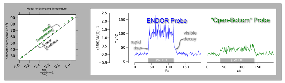
Figure 3: The simulated data in the left pane demonstrates how the short saturation-recovery $T_{1}$ experiment can predict the temperature of the sample. The value $\left(M(t)/M(0)\right)-1$ is the relative difference in the observed signal, $M(t)$. This plot assumes an initial temperature of $\sim 25^{o}$C, and thus an assumed initial $T_{1,0}$ of $\sim 2.5\;\mbox{s}$. The right pane displays the time-dependent response of the heating while cycling the microwave power from off to on. Data are presented both for the previously described home-built (“open-bottom”) probe design [6, 1, 42], as well as a sample positioned inside an ENDOR cavity. We find that the relatively ad-hoc, home-built “open-bottom” probe design demonstrates less sample heating than the commercial ENDOR setup. In addition, the time-dependent measurement of temperature in the ENDOR setup shows a decay that stretches over a few seconds, while this experiment cannot resolve the timescale of the temperature decay in the ad-hoc probe.

As discussed earlier, the measurements of $T_{1,0}$ can probe both the magnitude and the timescale of the change in sample temperature that microwave irradiation induces. We present two separate experiments, optimized, respectively, for measuring how the sample temperature varies as a function of the steady-state microwave power, as well as in time after a rapid change in microwave power.

A numerical calculation (left pane of fig. 3), based on the exponential $T_{1}$ decay (eq. 2) and the Hindman model (eq. 1) verifies that the relative change in magnetization, $\left(M(0)/M(T)\right)-1$, remains a linear function of temperature from 20^oC to 80^oC during the single-scan short-recovery $T_{1,0}$ experiments previously described in sec. II.1. This linear relationship relies on both the approximately linear dependence of magnetization on $T_{1,0}$ when short recovery delays are employed (here $\tau=0.5\;\mbox{s}\ll T_{1,0}$) and on the approximately linear dependence of $T_{1,0}$ on temperature.

These single-scan short-recovery $T_{1,0}$ experiments can quickly test the performance of the NMR probe configurations best suitable for ODNP experiments. Specifically, since a commercially designed ENDOR cavity has a built-in rf coil, we expected that it might present less perturbation of the electric field in the cavity, and so demonstrate less sample heating or a significantly faster temperature response than home-built ODNP probe designs. We performed the single-scan short-recovery $T_{1,0}$ experiment on water loaded into a capillary and placed inside a commercial ENDOR cavity (Bruker ER 801). In this setup, variable capacitors were added inside an aluminum box outside the cavity in order to tune and match the ENDOR rf coil so it could be used for NMR signal detection. In order to position the sample in the center of the cavity, a slightly larger capillary (1.2 mm o.d.) with one fused end holds the sample capillary (0.6 mm i.d. 0.84 mm o.d. quartz). We then compared the performance of this ENDOR probe to the home-built NMR saddle-coil probe design previously described in [6, 42, 2, 37]. After loading a sample capillary into a homebuilt NMR probe, we inserted it into a typical TE101 rectangular microwave cavity and again performed the single-scan short-recovery $T_{1,0}$ experiment. Surprisingly, the temperature of the sample in the home-built ODNP probe remains lower overall and responds on a similar or faster timescale than the temperature of the sample in the ENDOR cavity (fig. 3), i.e. presents better ODNP performance. This data also offers insight into the time that these ODNP probes need to equilibrate the temperature after the application of microwave irradiation. For both the ENDOR and the home-built setups, the temperature of the sample responds to changes in the microwave power within less than five seconds. Thus, we can acquire accurate ODNP enhancement values without including additional waiting periods longer than the length of the $5\times T_{1}$ recovery period, i.e. typically no more than 10-12 s.

Like others (e.g. [10]), we initially assumed that the transfer of heat through the capillary wall does not likely vary significantly between different probes and hardware setups. However, the unexpected difference in sample heating observed in the ENDOR vs. home-built probe indicates that the difference in their heat transfer can be significant. Specifically, in the ENDOR setup, two layers of quartz (the sample capillary wall and the wall of the outer capillary used for positioning) and an intermediate, insulating layer of air come between the cooling air and the sample. We hypothesize that this insulation may cause increased heat retention in the sample. This would imply that the transfer of heat through the capillary wall contributes significantly towards cooling the sample and should be considered when designing an ODNP probe.

With this knowledge, we present an ODNP probe in which the NMR probe and sample are contained inside a 3 mm quartz tube that passes entirely through the top and bottom openings of the microwave cavity (“pass-through design”). In the previously described home built design (i.e. “open-bottom design”), the sample tube and rf coil protrude from an enclosed glass tube that is held in the cavity from the top, and where the cooling air enters the cavity through the microwave waveguide on the side of the cavity. Therefore, small variations in the iris coupling and sample positioning can lead to variation in the air-flow near the sample. In the new pass-through design, air flows through the 3 mm quartz tube, and thus over and across the NMR coil and sample capillary (0.6 mm i.d. 0.84 mm o.d. quartz, for both designs), resulting in more consistent sample cooling. Additionally, in the previously described “open-bottom” design, only the collet at the top of the cavity stabilizes the sample position, while the pass-through design holds the sample tube more firmly and reproducibly at the center of the cavity by fastening at the top and bottom, preventing radial displacement of the sample capillary.

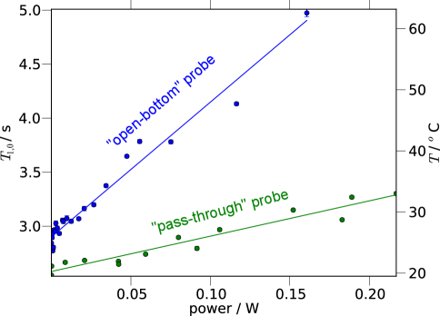
Figure 4: A series of experiments show how the $T_{1,0}$ of pure water increases with increasing microwave power for two different hardware setups. The model of fig. 1 (from [23]) then converts the $T_{1}$ values to temperatures ($y-$axis on the right). Even with cooling air, the temperature can increase significantly with power in the open-bottom setup (design presented in previous publications [6, 1, 42]) and the curve presented here can vary dramatically as the probe position or the cavity matching changes. However, the improved pass-through probe design [43] reduces the heating to a reproducible level that is less than the lowest heating seen with the open-bottom design, while retaining the same sample size of 3.5 µL and a design that one can insert into any functioning cw ESR cavity. Most importantly, the method illustrated here allows us to intrinsically probe the sample heating and will permit the development of further improved systems.

We measured the $T_{1,0}$ time (eq. 2) of water inside the new pass-through probe design as a function of incident microwave power. The Hindman model (fig. 1) can then determine the sample temperature from the value of $T_{1,0}$ (fig. 4) at each microwave power increment. These measurements (fig. 3) confirm the significantly reduced sample heating with the pass-through probe design relative to the previously presented open-bottom design from [42]. Likely, both the more consistent positioning of the sample in the area of minimal electric field and the more consistent air cooling contribute to the improved performance of the pass-through probe (cf. fig. 4). Furthermore (not shown in this plot), in repeated measurements, the pass-through probe presents a reproducible dependence of temperature on microwave power. By contrast, upon removing and reinserting the NMR probe, measurements taken with the open-bottom design can vary significantly. In fact, the variation of sample heating due to small changes in the sample positioning proves more problematic than the overall increase in the amplitude of sample heating itself. This is because the irreproducible variations in heating seen with the open-bottom design block any attempts to systematically correct for the change in $T_{1,0}$ as a function of power, while one can correct for reproducible heating effects, as will be shown.

In summary, the $T_{1,0}$ of water allows us to identify the experimental setup that optimizes the $B_{1,\mu w}/E_{\mu w}$ ratio ($B_{1,\mu w}$ and $E_{\mu w}$ are the microwave magnetic and electric field amplitudes, respectively). In consequence, this procedure allows one to optimize the ratio of the saturation, $s(p)$, to the dielectric heating. However, even in an improved setup, the dielectric heating still introduces measurable changes in the bulk water relaxation time. In turn, the theory predicts that these changes lead to measurable changes in the signal enhancements, especially for samples with low concentrations (i.e. $\leq 500\;\mbox{\textmu M}$) of nitroxide spin probes.

III.3 Observation of Enhancements and Relaxation Times

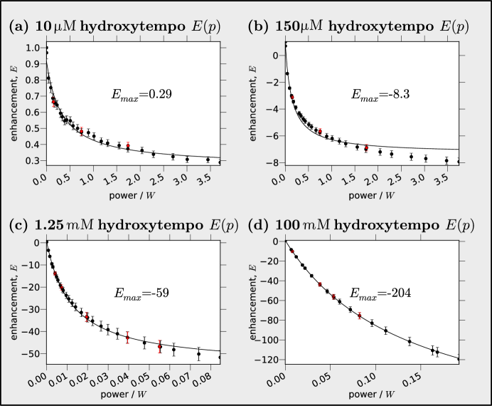
Figure 5: These plots show the ODNP signal enhancement, $E(p)$, as a function of power, $p$, for three different concentrations of 4-hydroxy-TEMPO spin probes dissolved in water. We integrate the enhanced signal intensity and normalize it against the unenhanced signal intensity (i.e. $E(0)=1$) in order to determine the unitless value of $E$ displayed along the $y-$axis. The solid lines show the best fit to the uncorrected model (eq. 9). The 100 mM sample follows the expected functional form, while the 150 µM sample clearly does not. Because of the residual misfit, we can only assign a rigorous meaning to the $E_{max}$ for the 100 mM concentration sample, where it gives the value that the enhancements asymptotically approach with increasing microwave power. For all the data, the repetition delay, $t_{rd}$, between NMR scans satisfies $t_{rd}>5T_{1,max}$ (see eq. 18) in order to prevent artifactual suppression of the enhancements at higher powers (as in fig. 2), while the dense sampling of data points plays a critical role in clearly identifying the misfit to the uncorrected model that occurs at the lower concentrations. The spectrometer acquires the black points in order of increasing microwave power; to check for reproducibility (e.g. lack of sample loss during the experiment), it then acquires the red (gray) points in order of decreasing microwave power.

Eq. 20 predicts that the enhancements observed for low concentration samples at higher microwave power will present a non-asymptotic (approximately linear) dependence on the microwave power. As a result, they should deviate significantly from the uncorrected model (eq. 9).

To test this prediction, we acquired the enhancement vs. microwave power, $E(p)$ (fig. 5), curves for three different concentrations, 150 µM, 1.5 mM, and 100 mM, of 4-hydroxy-TEMPO spin probes freely dissolved in water (fig. 5). At a 100 mM concentration of free spin probe, where $k_{\rho}CT_{1,0}\sim 100\gg 1$, we expect the leakage factor to remain constant with power. Thus, the uncorrected model (eq. 9) should still predict the enhancements accurately. Indeed, the observed ODNP signal enhancements fit well to the expected asymptotic curve (depicted with the solid line), which extrapolates to an $E_{max}$ of -204. This $E_{max}$ value agrees reasonably with recent literature data that draws from pulsed ESR and FCR measurements [10], while significantly exceeding previous predictions gleaned from cw ODNP measurements [6]. However, for samples with 150 µM free spin probe concentration and lower, where $k_{\rho}CT_{1,0}\leq 0.15\ll 1$ (cf. eq. 20), even the best fit of the enhancements ($E(p)$) to the uncorrected model does deviate significantly (fig. 5b), as predicted by eq. 20.

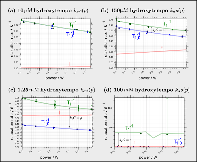
Figure 6: These plots show the variation of the bulk relaxation rate, $T_{1,0}^{-1}$, total relaxation rate, $T_{1}^{-1}$, and leakage factor, $f$, as a function of microwave power for four different concentrations of spin probe. We will shortly show that by accounting for the decrease in $T_{1}^{-1}$ as a function of microwave power, the corrected model removes the misfit to the uncorrected model that we displayed in fig. 5. These plots also allow one to track the dipolar self-relaxation rate, $\rho=k_{\rho}C$, which is the difference between the total ($T_{1}^{-1}$) and bulk ($T_{1,0}^{-1}$) relaxation rates and graphically appears as the distance between the two respective lines (black arrow). This data does not exclude the possibility that $\rho$ might slightly vary with power at high concentrations. However, at low concentrations, which are more important to biological studies, any change in the self-relaxivity, $k_{\rho}$, with increasing microwave power is insignificant compared to the change in $T_{1,0}$ and microwave power. By calculating the power variation of $f=\rho/T_{1}^{-1}$, we can see how dielectric heating impacts the leakage factor differently for different concentration of spin probe. At high spin probe concentration (100 mM), the leakage factor, $f$, does not vary significantly, since it has a value of $f\approx 1$ for all microwave powers, which is why the high probe concentrations demonstrate close adherence even to the uncorrected model (fig. 5). By contrast, at low concentration, the leakage factor varies significantly, exhibiting an approximately linear dependence on power (as derived by eq. 20).

In a similar fashion, we can acquire the total relaxation rate, $T_{1}^{-1}(p)$, as a function of power, and compare it to the bulk water relaxation rate, $T_{1,0}^{-1}(p)$. This allows us to estimate the leakage factor, $f$ (in fig. 6). As predicted by eq. 19, $f$ changes as a function of microwave power for lower concentrations, while remaining consistently close to 1 for all microwave powers at very high concentrations (approaching 100 mM, where $k_{\rho}CT_{1,0}\gg 1$). The relaxation data of fig. 6 also allows us to analyze the assumptions of the corrected analysis, so that we can understand these assumptions before proceeding to apply the corrected analysis to extract hydration dynamics information. In particular, (like the uncorrected analysis) the corrected analysis does not account for how dielectric heating might alter the self-relaxivity, $k_{\rho}$, and cross-relaxivity, $k_{\sigma}$ (table 2). We can measure the self-relaxation rate, $\rho=k_{\rho}C$, which (following eq. 16) is the difference between the total relaxation rate, $T_{1}^{-1}$, and the bulk water relaxation rate, $T_{1,0}^{-1}$, as shown in fig. 6. The observation of this value confirms an important feature of the corrected model. Namely, at low spin probe concentrations ($<2\;\mbox{mM}$) the sizable variation in the bulk water relaxation rate ($T_{1,0}^{-1}$) with microwave power by far exceeds any variation of the self-relaxation rate ($\rho=k_{\rho}C$), so that any variation in $k_{\rho}$ with temperature is insignificant.

Surprisingly, these observations do contradict the intuitive notion that dielectric heating should primarily effect changes in the parameters traditionally regarded as containing all of the dynamic information relevant to the Overhauser effect: namely, the self-relaxivity (typically simply called the relaxivity), $k_{\rho}$, the cross-relaxivity, $k_{\sigma}$, and, the ratio between these two values, the coupling factor, $\xi$. This is because uniformly, and especially at biologically relevant lower concentrations ($\leq 500\;\mbox{\textmu M}$) of nitroxide probes, heating-induced variation in the relaxivities that encode the local dynamic information plays a far less important role in determining the ODNP signal enhancements than does heating-induced variation in the bulk water relaxation, $T_{1,0}^{-1}$. Obviously, in cases where one employs cw ODNP to measure hydration dynamics with spin probe concentrations greater than 1 mM (where $k_{\rho}C$ begins to dominate the relaxation rates), or when more advanced instrumentation allows one can distinguish more subtle changes in relaxivity, one may wish to revisit variation of $k_{\rho}$ and $k_{\sigma}$ with microwave power as a secondary correction. (Bennati et. al. have already performed extensive modeling, based on FCR data [12] that would assist in such an effort.) However, currently, the most important step in compensating for small, residual sample heating is that of correcting for the variation in the bulk water relaxation.

III.4 Separate Calculation of $k_{\sigma}$ and $k_{\rho}$

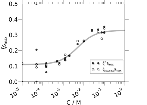
Figure 7: This figure presents a series of (unaveraged and uncorrected) measurements of $\xi s_{max}=k_{\sigma}s_{max}/k_{\rho}$ calculated by two different methods. First, we determined $(1-E_{max})/T_{1}(0)$ (i.e. uncorrected $k_{\sigma}s_{max}$) and $k_{\rho}$ eq. 32 from each sample independently. The ratio of the two yields the (closed circles) $\xi^{*}s_{max}$ values presented, where we use the star to indicate that $\xi^{*}$ was extracted by the ill-determined method. Note that, in the terminology of the standard uncorrected analysis, $\xi^{*}s_{max}=(1-E_{max})/f$. The resulting data has very high scatter at low concentration – note in particular the outliers prevalent at lower spin probe concentration, $C$, of which the values lying at the limits of the $y$-axis have been thresholded, since the calculated values have such high errors that they are not physically realistic. In the second set of data ($\xi_{accurate}s_{max}$, open circles), we calculate $k_{\sigma}$ in the same way, but always use an average value of $k_{\rho}$ determined from higher concentration data. The gray line gives 0.33 $s_{max}(C)$, where $s_{max}$ is given by eq. 31, with the value of $b^{\prime\prime}$ as determine by Bennati et. al. [11]. Note that the value of $b^{\prime\prime}$ determines the concentration at which the inflection point (near a concentration of 4 mM) of the gray curve occurs; the fact that the data follows the curve through its inflection point means that the value of $b^{\prime\prime}$ is similar to that predicted by a ratio of the rates measured in [11].

The study by Armstrong and Han [6] obtains $\xi$ by extrapolating a relatively evenly spaced series of concentrations between 0 and 15 mM, and is thus heavily weighted by the low concentration values. This led us initially to hypothesize that the difference between the higher coupling factor of 0.33 [10] and the lower value of 0.22 [6] arose from the fact that, at very low concentration, some finite population of bulk water does not diffusively exchange with the water near the spin probe on a timescale less than the NMR $T_{1}$ time; this would result in having a continuum of different water populations with slightly different enhancement values, and would have the effect of lowering the enhancement at low concentration. Rudimentary calculations led to the conclusion that this effect did not play an important role.

To investigate this issue further, we can ask what might be gained by separately calculating the cross-relaxivity, $k_{\sigma}$, and the self-relaxivity, $k_{\rho}$, as previously described in the theory section. Fig. 7 shows the same raw data processed in two ways. In one case, we calculate the product of the coupling factor and the saturation factor, which we denote with $\xi^{*}s_{max}(C)$ (where the star – or lack of – indicates the method of processing) to indicate an ill-determined $\xi^{*}$ value, which follows the calculations used in previous studies. For the second case, when we determine $\xi s_{max}(C)$ via the corrected analysis, we acknowledge that $k_{\rho}$ determined from the low-concentration samples has a very high percentage error; the error comes from the fact that the total $T_{1}$ relaxation is dominated by the bulk water relaxation, $T_{1,0}$ so that $k_{\rho}C$ is difficult to determine (cf. eq. 16 – because the difference between $T_{1}^{-1}$ and $T_{1,0}^{-1}$ in eq. 25 is very small and is divided by a very small concentration, $C$). Thus, a value for $k_{\rho}$, taken from an average of the higher concentration data, should be more accurate. In fact, when we apply this value of $k_{\rho}$ for the calculation of all $\xi s_{max}$ values at all concentrations, the scatter of the data is dramatically reduced, and even at concentrations as low as 10 µM, a clear and meaningful trend becomes apparent.

Interestingly, without further correction, the shape of $\xi s_{max}$ vs. spin probe concentration matches the predictions of Bennati et. al. [12, 11]. Thus, this data unequivocally supports the higher value of 0.33 as the correct value for the coupling factor between water and freely dissolved spin label, as opposed to the lower value of 0.22 previously used as a reference. This data also appears to support a value of $b^{\prime\prime}/C$ (i.e. the ratio of the Heisenberg spin exchange and electron spin relaxation rates in eq. 31) that is at least the same order of magnitude as the value of $198.7\;\mbox{M}^{-1}$ determined from the data of Türke et. al. ([11]).

This leads to the remaining hypotheses that either the results of Armstrong and Han [6] are strongly affected by the presence of dimethyl-sulfoxide in their solution (i.e. that it genuinely perturbs the hydration dynamics), that the artifact noted earlier (arising from the significant lengthening of the $T_{1,0}$ with microwave power) resulted in artificial suppression of the signals at high microwave powers, or that one or both of these effects combine with a large error when extrapolating measurements of $\leq 15\;\mbox{mM}$ to $s_{max}$ at high concentration. Low concentrations of $\leq 15\;\mbox{mM}$ may not be a sufficiently high spin probe concentrations for extrapolating to high concentration, and may lead to large errors either when explicitly extrapolating $s_{max}$ to high concentrations, or when implicitly doing so by extrapolating $E_{max}$ to high concentrations, as done in [6]. Regardless, these results support the conclusion that the higher measured value of the coupling factor, 0.33 [12, 11, 10], is indeed the correct value for the coupling factor between water and freely dissolved, small nitroxide spin probes, and that even rudimentary cw DNP instrumentation and analysis can quantify this value without the need for pulsed ESR and/or FCR instrumentation.

III.5 Application of the Improved Analysis

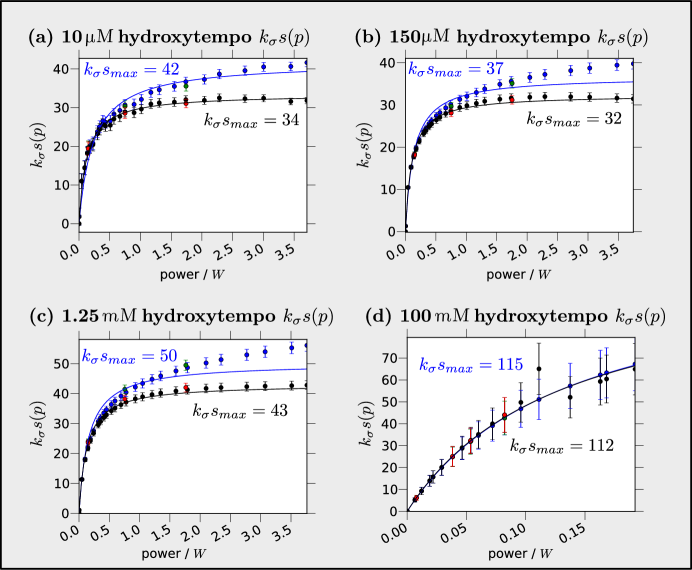
Figure 8: These plots present the product of the cross-relaxation with the electron saturation factor, i.e. $k_{\sigma}s(p)$, for the same series of experiments as fig. 5. The uncorrected curves, in blue (gray), present $(1-E(p))/T_{1}(0)$ and so have the same shape as the curves in fig. 6 (though inverted); note that – due to the imperfection in the uncorrected model – these are only apparent values of $k_{\sigma}s(p)$. The black curves and points present the $k_{\sigma}s(p)$ product, as determined by the corrected analysis (i.e. $(1-E(p))/T_{1}(p)$ as determined by eq. 29,24,26). With knowledge of the maximum possible saturation factor, $s_{max}$, one can extract the coupling factor directly from the fit shown (as in table 3). The corrected data for the low concentration samples clearly level off at high microwave power, indicating that the highest microwave powers employed here significantly saturate the electron spin transition. Even at low concentration, the uncorrected data never level off, since heating induces a continuous increase in the leakage factor, resulting in a continuous increase in enhancements. The data for the higher concentration samples do not level off simply because ESR transitions require the application of more intense microwave radiation before they saturate appreciably (i.e. $p_{1/2}$ is greater as a result of the fast Heisenberg exchange and subsequent broad ESR linewidth). The three sets of data fit to different values of the $k_{\sigma}s_{max}$ value because $s_{max}$ remains closer to $1/3$ at low concentration, while at high concentrations, Heisenberg exchange drives $s_{max}$ close to 1.

We can now analyze the difference between the uncorrected analysis (eq. 9,11), and the analysis that corrects for the dielectric heating effect (eq. 29,30). As reviewed previously, whether one seeks to retrieve the translational correlation time, $\tau_{c}$, or the local translational diffusivity of the hydration water, $D_{local}$, one first needs to extract an accurate value for the coupling factor, $\xi$. The uncorrected analysis employs the $E(p)$ curves and $E_{max}$ values of fig. 5 directly to calculate the hydration dynamics via eq. 11. However, in order to compare the two models on an equivalent basis, we employ eq. 29. For the uncorrected model, we plot $k_{\sigma}s(p)=\left(1-E(p)\right)/T_{1}(0)$, where $E(p)$ is the data of fig. 5 and $T_{1}(0)$ is the NMR longitudinal relaxation time in the absence of microwave power. We then measure $T_{1}(p)$, interpolated where necessary via eq. 24 and 26, as shown in fig. 6. We insert the interpolated $T_{1}(p)$ values into eq. 29 and plot the resulting corrected $k_{\sigma}s(p)$ values in fig. 8 as well.

At 100 mM, and, to a lesser extent, at 1.25 mM spin probe concentrations the $k_{\sigma}s(p)$ curves generated by both models match closely for all microwave powers (fig. 8d). The high spin probe concentration leads to a fast self-relaxation rate, $k_{\rho}C$. Since the self relaxation rate, $k_{\rho}C$, does not exhibit large changes with microwave power, it masks the change in the bulk water relaxation rate, $T_{1,0}^{-1}$, with microwave power.

At the lower concentrations of 10-150 µM, the $T_{1}$ time changes significantly with microwave power (as seen in fig. 6). Therefore, the apparent values of $k_{\sigma}s(p)$ that the uncorrected model generates differ significantly from the corrected values of $k_{\sigma}s(p)$. Most significantly, the data generated by the corrected analysis (eq. 29,30) indeed level off visibly upon saturation of the ESR transition at high microwave power (fig. 8a-b), as predicted by the asymptotic model for ESR saturation (eq. 8). These corrected data should therefore remain consistent despite any changes in the hardware parameters, which would affect only $\Delta T_{1,0}$. The corrected values of $k_{\sigma}s(p)$ will also contribute less error associated with misfit to the model. Finally, since the corrected values of $k_{\sigma}s(p)$ level off at high power, we gain confidence that they approach the asymptotic $k_{\sigma}s_{max}$ value closely, and that extrapolation to infinite power will generate less error. These two gains in accuracy become more significant at lower spin probe concentrations and at higher microwave powers.

We can also address the question of whether or not dielectric heating might alter the fundamental relaxation rate, $k_{\sigma}$. Interestingly, the fact that all the data fit well to the corrected model implies that $k_{\sigma}$ does not vary significantly as a function of microwave power.

Table 3 collects the numerical results from these experiments. Like in our initial analysis, these data support the higher coupling factor value of 0.33. We should note that additional experiments (data not shown) were done to verify that we choose a field relative to the cavity frequency that is positioned exactly on the ESR resonance. We also note that the error analysis of the fitting procedure is relatively complex, and will be the subject of future publication.

	10 µM		150 µM		1.25 mM		100 mM
	uncorrected	corrected	uncorrected	corrected	uncorrected	corrected	uncorrected	corrected
$k_{\sigma}s_{max}$ / $\mbox{s}^{-1}\mbox{M}^{-1}$	42	34	37	32	50	43	115	112
$s_{max}$[11, 9]	—- 0.334 —-		—- 0.352 —-		—- 0.465 —-		—- 0.968 —-
$k_{\sigma}$	126	102	105	91	107	92.7	119	116
$k_{\rho}$ / $\mbox{s}^{-1}\mbox{M}^{-1}$	—- (-137) 353.4 —-		—- (391) 353.4 —-		—- (357) 353.4 —-		—- 353.4 —-
$\xi$	0.36	0.29	0.30	0.26	0.31	0.26	0.34	0.33
$\xi^{*}$	(-0.94)	(-0.74)	(0.27)	(0.23)	(0.30)	(0.26)	(0.34)	(0.33)
$\tau_{c,bulk}$/ ps	26	47	44	59	40	58	31	34

Table 3: This table gives the cross relaxivity, self relaxivity, and coupling factor for the dipolar interaction between water and free spin probes at ambient temperature, measured at four representative 4-hydroxy-TEMPO spin probe concentrations. The gray numbers in parentheses present the inaccurate values that result from attempting to calculate $k_{\rho}$ from samples with very low concentrations of spin probe (i.e. where eq. 25 has a significant error), as previously discussed. As also demonstrated in fig. 7, the resulting attempt to calculate a value of $\xi^{*}$ gives data with sometimes physically unrealistic values (as seen here since $\xi$ must lie in the range $0<\xi<0.5$). Therefore, we focus on the data for the four representative 4-hydroxy-TEMPO spin probe concentrations, where we have employed the value of $k_{\rho}$ measured at 100 mM. We calculate a value of $\xi$ both with and without the correction for the change in the $T_{1}(p)$ times as a function of power (as given by eq. 29 and fig. 8), labeled as “corrected” and “uncorrected,” respectively. Note that at low concentrations, where the bulk water relaxation is more important, the correction is more significant. The various rows of this table outline the various steps of the corrected analysis, as given at the end of the theory section II.3.4; the values of $s_{max}$ are calculated via. eq. 31, with $b^{\prime\prime}/C=198.7\;\mbox{M}^{-1}$. At all concentrations, the measured values of the coupling factor, $\xi$, more closely agree with the values of Bennati et. al. [11], as well as the values predicted by FCR [1, 12] and MD simulations [13], than those previously extrapolated by Armstrong et. al. [1, 6]. It is important to note that the difference in the coupling factor measured at different concentrations does not indicate whether or not the corrected data is accurate; rather correcting for the variation of $T_{1}(p)$ with microwave power must always generate results that are more accurate than when such a correction is not performed.

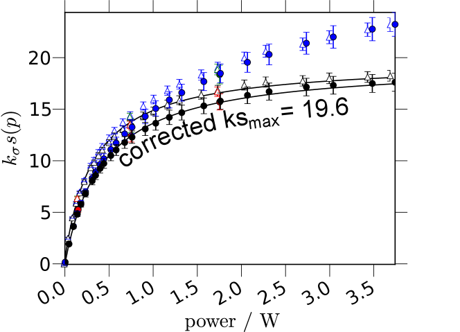
Figure 9: This demonstrates the effect of the corrected analysis on an ODNP measurement taken for a mixture of tethered TEMPO label (3% mole ratio) embedded in a DOPC lipid. Since a chemical bond attaches it to the very large vesicle membrane, we expect the spin probe to exhibit an $s$ of near 1 (as shown in [6]) leading to $k_{\sigma}s_{max}\approx k_{\sigma}$. This is confirmed by the fact that a solution containing 32.0 mM lipids (circles) and a 4.89 mM lipids (open triangles), i.e. 9.6 mM and 150 µM of spin probe, yield closely agreeing $k_{\sigma}s_{max}$ values of 19.6 and 19.5, respectively. The values plotted here are scaled by the $T_{1}$, following eq. 29. Therefore, despite the similar appearance of the two lines, the 32 mM sample does indeed exhibit much higher values of enhancements ($E_{max}\approx-20$) than the diluted sample ($E_{max}\approx-4.9$). For clarity, we have omitted the best fit lines for the uncorrected data in blue (gray), which – like for the free label – exhibits misfit beyond the bounds of the experimental error. The best fit values for the uncorrected $k_{\sigma}s_{max}$ are 24.5 $\mbox{s}^{-1}\mbox{M}^{-1}$ for the 32 mM DOPC sample and 23.2 $\mbox{s}^{-1}\mbox{M}^{-1}$ for the 9.6 mM DOPC sample (we use the average value of 23.9 $\mbox{s}^{-1}\mbox{M}^{-1}$ in the analysis in the text). The slight difference in the powers at which the two samples saturate likely indicates a slight difference in the $B_{1}$ conversion ratio (related to the cavity $Q$ factor) after loading the two samples.

III.6 Application to a Sample with Tethered Spin Probes

An application of the new analysis to an example biological system helps to clarify the importance of the preceding results. We selected 200 nm diameter unilamellar vesicles made of DOPC lipid, dissolved in water at two different concentrations: 4.89 mM and 32.0 mM. We perform inversion recovery measurements to determine the value of $T_{1,0}(p)$ as a function of microwave power, $p$. For the ODNP (i.e. $E(p)$) and $T_{1}(p)$ measurements, we prepare another sample that also includes 3 mole % of a lipid with a tethered nitroxide probe located at the surface of the lipid bilayer.

Biologically relevant systems with tethered spin probes tend to give results that one can interpret in a more straightforward manner than one can interpret the results from freely dissolved spin probes. Specifically, because the tethering to larger biological systems restricts the TEMPO spin probe dynamics, we can assume that nitrogen relaxation drives $s_{max}$ to closely approach 1, as explained in [6]. It follows that the extrapolated value of $k_{\sigma}s_{max}$ conveniently approximates the cross relaxivity, $k_{\sigma}$.

At the same time, the same motional restriction also typically causes tethered spin probes to exhibit a faster ESR relaxation time than untethered spin probes and thus makes the ESR transition harder to saturate. Specifically, notice how $k_{\sigma}s(p)$ for a free spin probe of 150 µM concentration in fig. 8b begins to level off near 1 W of microwave output power, while the $k_{\sigma}s(p)$ values for the 4.89 mM sample of DOPC with a spin probe concentration of 150 µM do not begin to level off until about 3 W, as presented in fig. 9. The experiments on DOPC here employ approximately the same range of power as the free spin label studies presented earlier in this publication. Arguably, the free spin label studies exceed the powers strictly necessary to achieve clear ESR saturation at low concentrations when they employed microwave output powers of up to 2-3 W. However, for the ODNP study of the lipid vesicle surface, enhancements must be acquired at output powers approaching 3 W before saturation becomes evident. The use of such high powers can lead to rather significant heating effects, making the corrected analysis even more important to quantitatively determining the coupling factor. In the case of the DOPC sample, we observe an uncorrected value of $k_{\sigma}s_{max}\approx k_{\sigma}$ that differs from the corrected value by more than 20%.

Like in the free spin probe study, in order to avoid using an ill-determined leakage factor, we do not calculate $\xi$ for the uncorrected analysis from $\left(1-E_{max}\right)/659.32f$. Rather, we first determine the value of $k_{\sigma}$ for both the corrected and uncorrected analyses. Then, we compare the $T_{1}$ times of the labeled and unlabeled samples in the absence of microwave power from the 32 mM sample, namely 314 $\mbox{s}^{-1}\mbox{M}^{-1}$, in order to retrieve a reliable value of $k_{\rho}$ that we can use to calculate the coupling factor from eq. 22 ($\xi=k_{\sigma}/k_{\rho}$), for both the high and low concentration samples (following eq. 32). We retrieve a corrected value of the coupling factor $\xi=0.062$, while we retrieve an uncorrected value of 0.076.

Similarly, we can determine the value of $\tau_{c,site}$ corresponding to $\xi_{site}$, which is measured at a local site in or on the macromolecule where the spin probe is tethered. The corrected vs. uncorrected analyses measure different values for $\xi_{site}$ (fig. 9), leading to correlation times of 226 ps vs. 263 ps, respectively. In previous work, researchers determined $\xi_{site}$ based on the uncorrected analysis; through the discussions and demonstrations presented here, it is clear that the corrected analysis should be used instead. The correction of the value of $\xi_{site}$ implies a measurable correction for the local translational diffusion coefficient. Insertion of the two values for $\tau_{c,site}$ into eq. 33 determines that, in this case, the two values of $D_{local}$ generated from the corrected and uncorrected analyses differ by more than 16%. Since other samples with tethered spin probes should present similar ESR and ¹⁴N relaxation times, we expect them to exhibit similar differences. Thus, previous ODNP studies presenting relative trends for the $\xi_{site}$, $\tau_{c,site}$ or $D_{local}$ values remain valid, but their absolute values need to be cautiously reexamined, as will be further detailed.

One should remain cautious that even the corrected method laid out here might not apply in a straightforward fashion to chemical systems where the small residual changes in temperature with increasing microwave power might induce a transition in the structure and dynamics of the sample. Fortunately, most or all previously investigated samples that one would suspect of presenting such problems – such as macromolecules that undergo a glass transition [5, 37], or proteins that undergo aggregation [2], folding, or unfolding [3] – the transition temperature does not fall between room temperature and the temperature at the maximum microwave power ($\approx 35^{o}C$). However, even in other systems that undergo transitions within the experimental temperature range, the methodology presented here should remain very useful by registering and highlighting any sudden changes in $k_{\rho}$ and/or $\xi$ as an unexpected change in $\xi s(p)$ (i.e. misfit to the corrected model) with increasing microwave power, $p$.

III.7 The Corrected Analysis in Context

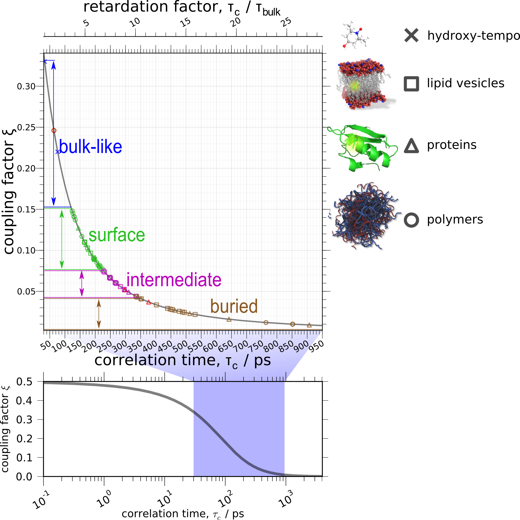
Figure 10: Here, we collect data for the coupling factor, $\xi$, between a spin probe attached to specific, known biological sites and the nearby (within 5-10 Å) hydration water. Even though these data come from previous publications that employ the uncorrected analysis, the results reproducibly fall within a particular zone corresponding to the spin probe location (i.e. exposed, intermediate, or buried as defined in the text). The exceptions to this trend are the lipid. The vesicle doxyl-stearic acid labels (not shown) consistently show significantly higher dynamics than their tempo-PC analogs (which are presented in this plot). Hyaluronic acid [4], a polyelectrolyte which exhibits exceptionally fast, i.e. bulk-like, dynamics. The unfolded protein mfp151 [4], exhibits buried-like dynamics, and because of this is believed to have a some amount of local structure near the spin labeled site [4]. The native (i.e. folded) state V66R1 site in ApoMb (Apo-myoglobin) [3] exhibits intermediate dynamics, even though it is believed to be on the surface of the protein. The retardation factor $\tau_{c}/\tau_{c,bulk}=D_{H_{2}O}/D_{local}$ gives the slow-down of the translational hydration dynamics relative to bulk water; the measurement for $\tau_{c,bulk}$ sets the value of 1 on the retardation axis and, therefore, for the absolute values of the diffusivities. Both the correct value (at $\tau_{c}/\tau_{c,bulk}=1$) and the previously employed value (at $\tau_{c}/\tau_{c,bulk}=2.3$) are shown above with a blue “x” above. Of course, if the previously employed value were used to set the value of 1 on the retardation axis, the value of the diffusion would change for all the data points shows.

In this section, we can now analyze how the new methodology will lead to a reinterpretation or adjustment of previously acquired results. Specifically, we will present how corrections for sample heating can lead to changes in the values determined for the coupling factor, $\xi$, in a given study. Here, an important parameter of biophysical significant is the retardation factor of the ODNP-measured translational diffusion dynamics near a spin probe functionalized onto a biomolecular system, relative to that of bulk water. In order to extract such retardation factors, we need to accurately determine the coupling factor between the freely dissolved spin probes and bulk water, which we use to quantify the translational correlation time, $\tau_{c,bulk}$. Past studies have had much greater difficulty in employing the uncorrected analysis to extract consistent values for the translational correlation time of water interacting with freely dissolved spin probes than in employing the uncorrected analysis to extract consistent values for the translational correlation time of water interacting with spin probes tethered to macromolecules. Previous ODNP dynamics studies (excluding [4, 37]) employ a relatively low value of 0.22 as the reference value for the coupling factor of bulk water. Eq. II.3.4 implies that this corresponds to a translational correlation time of $\tau_{c,bulk}=76\;\mbox{ps}$. However, the results here clearly support the higher bulk water coupling factor of 0.33, which rather implies (via. eq. II.3.4) a choice of $\tau_{c,bulk}=33.3\;\mbox{ps}$. Eq. 33 points out that the local diffusivities, $D_{local}$, for all soft matter and biological samples are approximately proportional to the ratio of the coupling factor in freely diffusing water, $\tau_{c,bulk}$, to the coupling factor within a local volume around the tethered spin probe in a particular sample, $\tau_{c,site}$. Therefore, a choice of the higher (and correct) reference value of the bulk water coupling factor means that the values of $D_{local}$ for all samples are about two-fold slower relative to bulk water than was previously thought.

Given the existing controversy on the bulk water coupling factor, most ODNP studies in the literature anticipated such a dilemma. Therefore, they reported local hydration dynamics in terms of the translational correlation times, $\tau_{c,site}$, rather than in terms of the local hydration water diffusion coefficient, $D_{local}$, since the value of $\tau_{c,site}$ does not depend on the bulk water coupling factor. Since we have found unequivocal agreement that the bulk water coupling factor is $\xi_{bulk}=0.33$, we are now at liberty to use either $\tau_{c,site}$ or $D_{local}$, to describe the site-specific local hydration dynamics, depending on the context. However, as eluded to before, comparisons between the value of $D_{local}$ for the local translational hydration dynamics determined by different techniques are valid, while such comparisons based on the absolute value of $\tau_{c,site}$ are not necessarily valid.

The lower concentration ($\leq 1.25\;\mbox{mM}$) values in table 3 exhibit differences between the corrected and uncorrected values of 15 - 20%, while, as noted before, the DOPC sample exhibits a heating correction of greater than 20%. Therefore, we expect if samples were re-analyzed with the corrected analysis, the value of the measured coupling factor would decrease by up to 20%, though this number may vary. On the one hand, the pass-through probe employed here significantly minimizes the potential amount of net heating in the system. On the other hand, the microwave powers and the Q of the cavity employed in previous studies likely varies with each study, and are not necessarily as high as those used here. Thus, one can predict that moving an experiment to a different instrument, or even positioning the NMR probe slightly differently, can easily induce changes in $\Delta T_{1,0}$. Either changes in $\Delta T_{1,0}$, or changes in the microwave powers sampled could cause the measured values of $\xi_{site}$ to vary. Furthermore, each different protocol may or may not have employed sufficiently long recycle delays (i.e. delays that exceeded $5\times T_{1,max}$ of eq. 18). Therefore, in addition to a systematic decrease in the measured values of $\xi_{site}$, the corrected analysis may lead to a decreased scatter in the coupling factor value for a given sample, especially for samples with low spin concentrations. Because the heating correction is on the order of 20% for the well-controlled hardware setup shown here, and – as previously noted – we expect the previous setups to be significantly less well-controlled, we believe that a conservative estimate of the scatter in the measurement of the coupling factor, $\xi_{site}$, is about 5%.

The corrected analysis should remove any dependence on $\Delta T_{1,0}$ to allow one to determine an absolute value of $\tau_{c,site}$ and $D_{local}$, and to accurately and reproducibly reduce the scatter across different protocols and instruments. However, despite the previous inaccuracy in the absolute values of $D_{local}$, previous publications reproducibly employ measurements of the coupling factor to identify meaningful and biologically significant trends and transitions associated with changes in the local hydration dynamics [4, 37, 3, 2, 5, 30]. Since these studies employ the uncorrected analysis, the successful identifications that they achieve depend on the consistency of various experimental parameters. In particular, the researchers who acquired the datasets for previous measurements empirically discovered the need to only compare coupling factors determined in precisely the same position in the same cavity, from enhancements acquired over the same sampling of microwave powers. Such an experimental scheme ensures relatively consistent heating effects, i.e. a relatively uniform dependence on $\Delta T_{1,0}$. Therefore, it is crucial to emphasize that all qualitative trends and comparisons within each dataset, as previously published, should remain after correction.

Finally, to alleviate concerns over comparing data that come from different studies (i.e. datasets), we analyze a subset of previously published studies to estimate an upper limit on the error associated with comparing these different studies. It is worth noting that most of the data we review here are acquired on the same microwave cavity and NMR probe design and come from samples with relatively high, $\geq 500\;\mbox{\textmu M}$, spin probe concentrations, where the correction to the $\xi_{site}$ values (and, therefore, the $\tau_{c,site}$ and $D_{local}$ values) should be smaller than for lower concentration samples. For all these samples it is also known whether the spin probe resides within the hydrophobic core of a macromolecule or near the surface of a macromolecule.

When we compare this collection of measurements (fig. 10), we find that we can sort the dynamics into four categories. With the exception of the polyelectrolyte hyaluronic acid, which exhibits very fast hydration dynamics [4], bulk water is the only sample to exhibit $\xi>0.15$. Thus, we can classify this zone ($\xi>0.15$) as “bulk-like,” i.e. significantly faster than the dynamics observed on any labeled compounds. Researchers have routinely observed values of the coupling factor $0.075<\xi<0.15$ for surface dynamics of macromolecular systems, including unfolded proteins and uncomplexed polyelectrolytes, as well as the surface of lipid vesicles, and folded globular proteins [4, 3, 37, 44, 30, 5]. Researchers have routinely observed value of the coupling factor $0.042<\xi<0.075$ for samples where one expects intermediate dynamics, including surface labeled vesicles in the presence of viscogens such as 20% PEG [4] or binding agents such as $\geq 35\;\mbox{\textmu M}$ P188 [37], lipid vesicles with spin labels attached at the carbon positions immersed five to ten C-C bonds into the lipid bilayer (i.e. for label molecules 10 Doxyl PC, 7 Doxyl PC, and 5 Doxyl PC) [5], and the surface of the partially folded molten globule state of ApoMb [3]. Researchers have routinely observed value of the coupling factor $\xi<0.042$ for samples where one expects the spin labeled site to be buried inside a macromolecular complex; such samples include complexed polyelectrolytes [44, 4], aggregated protein fibrils [4, 2], buried sites of natively folded and molten globule states of ApoMb [3], and lipid vesicles where the spin label is attached 14 bonds deep into the vesicle (i.e. 14 Doxyl PC) [5, 37].

Interestingly, at this level of resolution, the location (i.e. surface vs. buried) of the site under investigation seems to be the primary determinant of the translational hydration dynamics, regardless of whether the site resides on a protein, membrane vesicle, or polymer. Thus, the cw ODNP method can already classify the location of the site based on its hydration dynamics (fig. 10). With the improvements presented here, future studies will reproducibly resolve and classify sub-categories of dynamics, allowing us to map out the hydration-dynamics-based landscape of proteins, lipid vesicles, and other soft matter systems on a finer, absolute scale. Previous research suggests that changes in the surface hydration dynamics should correlate strongly with the interfacial forces that drive biological and polymeric transitions [45, 46, 39, 47, 48]. As seen from the ApoMb and vesicle data, interesting effects, such as protein folding and complexation, initiate at sites with intermediate-regime hydration dynamics. Therefore, there is particular interest in such high resolution investigations into the rich variation of the hydration dynamics within the intermediate regime.

IV Conclusions

The corrected analysis proposed here (eq. 29,30) represents a significant improvement in the ability of cw ODNP to accurately quantify hydration dynamics. It is the first model to fit accurately acquired (i.e. without artifacts) enhancement vs. power, $E(p)$, data for low ($\leq 500\;\mbox{\textmu M}$) concentrations of spin probes. The data also resolves the debate over the determination of the bulk water coupling factor, pointing out that the higher value (0.33, 0.33-0.35, 0.36, and 0.30 from [11], [12], [1], and [13], respectively), rather than one previously determined by Armstrong et. al. (0.22 from [1]), should be used as the reference value for measurements of hydration dynamics. Entirely cw ODNP instrumentation can retrieve the resulting high $E_{max}$ values, without the need for pulsed ESR instrumentation, despite previous predictions [1, 6]. From one point of view, this agreement supports the validity of the FCR, MD, and pulsed ESR measurements, which employ similarly high spin probe concentrations. From another point of view, it supports the validity of the experimental strategy proposed in [1], which employs solely cw ODNP hardware as a viable quantitative analytical tool for determining the coupling factor, $\xi$. This conclusion is particularly promising and advantageous to the ODNP and analytical biochemistry communities since, as previously mentioned, cw ODNP hardware requires significantly less user training and expenditure than pulsed ESR hardware, and thus is more broadly available.

The results presented here outline standard tests that will facilitate further hardware development and clarify how one can proceed further in the task of developing cw ODNP as a generally applicable, push-button analytical tool for the quantification of local hydration dynamics. For the development of new NMR probes and/or ESR cavities, the measurement of the longitudinal NMR relaxation of bulk water, $T_{1,0}(p)$, as a function of microwave power, $p$, gives a complete test of the hardware’s ability to regulate the sample temperature in the presence of the strong microwave fields. However, the results actually support a better and faster standardized test of newly implemented hardware systems – namely, the corrected cw ODNP analysis for $\leq 150\;\mbox{\textmu M}$ 4-hydroxy-TEMPO. The enhancements and relaxation times of such low concentration systems change significantly in order to clearly indicate any heating effects (as in fig. 5a), while at the same time indicating the relative power conversion ratio (inversely proportional to $\sqrt{p_{1/2}}$ on resonance) of the system. Therefore, this standardized test will give a clear and quick indication of both how much power the system requires before it will appreciably saturate the ESR transition, as well as how much dielectric heating the hardware subjects the sample to at the required powers.

Five clear conclusions dominate this presentation: by measuring the bulk relaxivity, one can intrinsically probe the sample temperature and thus develop the next generation of cw ODNP hardware; by measuring and accounting for $T_{1,max}$, one can acquire reproducible signal enhancement data for a particular system; by implementing the new analysis presented here, one can recover accurate values of $\xi$, even in the presence of moderate sample heating; by repeating measurements at high concentration carefully, cw ODNP can retrieve values of the coupling factor that do indeed agree with predictions given by pulsed ESR and FCR measurements taken at similar concentrations; finally, by independently measuring $k_{\sigma}$, one can access information about the translational dynamics, even at concentrations of less than a hundred micromolar, opening up opportunities to study a wide range of new systems of biological significance. In addition to the method of calculating the self-relaxivity, $k_{\rho}$, at high concentration in order to determine the coupling factor, $\xi$, this also opens up the possibility of independently verifying the concentration (for instance, by UV-visible or IR spectroscopy) and observing trends in a fashion similar to how trends are currently observed in the coupling factor.

The results here also make it clear what comes next in the task of developing cw ODNP as an analytical tool for the quantification of local hydration dynamics. Systematic comparisons between measurements taken on different instruments or microwave cavities should now agree quantitatively. In particular, experiments that observe the change in the coupling factor across the various frequencies possible with X-band equipment would offer interesting insight into how accurately the existing models describe the hydration dynamics and should be possible with tunable cavity setups (similar extensions for the S- through Q-bands would be similarly interesting). However, until now, an understanding of ODNP that was capable of reproducibly extracting dynamics under variable conditions of sample heating and cooling was lacking, while such variations inevitably occur in a cavity with a tuning range of several  GHz (compare to [42]). This study also paves the way for further improved methodologies that compensate for sample heating, if they prove necessary. As previously discussed, even the significant improvements developed here might not suffice for some particularly difficult systems. For such systems, a properly integrated and automated cryostat can adjust air surrounding the sample to a lower temperature that compensates for the microwave heating. One can iteratively optimize such a compensation against the criterion that the $T_{1,0}$ remains constant with increasing microwave power. Such a procedure should yield a completely stable sample temperature throughout the course of the ODNP experiment, and negate any concerns over changing sample temperature. The current study also points out the clear benefit of the development of an error analysis that properly accounts for, among other detailed effects, the correlated error present in the $E(p)$ data, as well as the development of software and hardware to more fully automate ODNP measurements. In particular, this data indicates that the primary bottleneck for quantitative accuracy in ODNP is the NMR relaxation (i.e. $T_{1}$) measurements; a detailed statistics would help to highlight this fact, and more importantly, help to identify experimental strategies where the impact of such errors on the ultimate value of $D_{local}$ were minimized. Finally, while previous studies could distinguish between surface, intermediate, and buried chemical sites on different systems, or compare the modulation in hydration dynamics within the same system, the new methodology presented here opens up the possibility of classifying different types of surface or buried sites based on more subtle differences in their local hydration dynamics reproducibly, i.e. even across different studies and instruments.

References

- Armstrong and Han [2009] B. D. Armstrong and S. Han, Journal of the American Chemical Society (2009).
- Pavlova et al. [2009] A. Pavlova, E. McCarney, D. Peterson, F. Dahlquist, J. Lew, and S. Han, Physical Chemistry Chemical Physics 11, 6833 (2009), ISSN 1463-9076.
- Armstrong et al. [2011] B. D. Armstrong, J. Choi, C. López, D. A. Wesener, W. Hubbell, S. Cavagnero, and S. Han, Journal of the American Chemical Society 133, 5987 (2011).
- Ortony et al. [2011] J. Ortony, C. Cheng, J. Franck, R. Kausik, A. Pavlova, J. Hunt, and S. Han, New Journal of Physics 13, 015006 (2011).
- Kausik and Han [2011] R. Kausik and S. Han, Physics Chemistry Chemical Physics c0cp02512g (2011).
- Armstrong [2007] B. Armstrong, The Journal of Chemical Physics 127, 104508 (2007).
- Bates and Drozdoski [1977] R. D. Bates and W. S. Drozdoski, Journal of Chemical Physics 67, 4038 (1977).
- Hausser and Stehlik [1968] K. H. Hausser and D. Stehlik, Advances in Magnetic Resonance 3, 79 (1968).
- Hyde et al. [1968] J. Hyde, J. Chien, and J. Freed, The Journal of Chemical Physics 48, 4211 (1968).
- Türke et al. [2010] M.-T. Türke, I. Tkach, M. Reese, P. Höfer, and M. Bennati, Physical Chemistry Chemical Physics 12, 5893 (2010), ISSN 1463-9084.
- Türke and Bennati [2011] M. Türke and M. Bennati, Physical Chemistry Chemical Physics (2011).
- Bennati et al. [2010] M. Bennati, C. Luchinat, G. Parigi, and M.-T. Türke, Physical Chemistry Chemical Physics : PCCP 12, 5902 (2010), ISSN 1463-9084.
- Sezer et al. [2009] D. Sezer, M. Prandolini, and T. Prisner, Physical Chemistry Chemical Physics (2009).
- Hofer et al. [2008] P. Hofer, G. Parigi, C. Luchinat, P. Carl, G. Guthausen, M. Reese, T. Carlomagno, C. Griesinger, M. Bennati, and P. Höfer, Journal of the American Chemical Society 130, 3254 (2008), ISSN 1520-5126.
- Lingwood and Han [2011] M. Lingwood and S. Han, Annual Reports on NMR Spectroscopy 73, 83 (2011).
- Villanueva-Garibay et al. [2010] J. Villanueva-Garibay, G. Annino, P. Bentum, and A. Kentgens, Physical Chemistry Chemical Physics 12, 5846 (2010).
- Cai et al. [2006] Q. Cai, A. K. Kusnetzow, W. L. Hubbell, I. S. Haworth, G. P. C. Gacho, N. Van Eps, K. Hideg, E. J. Chambers, and P. Z. Qin, Nucleic acids research 34, 4722 (2006), ISSN 1362-4962.
- Qin et al. [2007] P. Qin, I. Haworth, and Q. Cai, Nature Protocols (2007).
- Solomon [1955] I. Solomon, Physical Review 99, 559 (1955).
- Yin et al. [1987] J. J. Yin, M. Pasenkiewicz-Gierula, and J. S. Hyde, Proceedings of the National Academy of Sciences of the United States of America 84, 964 (1987), ISSN 0027-8424.
- Popp and Hyde [1982] C. Popp and J. Hyde, Proceedings of the National Academy of Sciences of the United States of America 79, 2559 (1982), ISSN 0027-8424.
- van Bentum et al. [2011] P. J. M. van Bentum, G. H. A. van der Heijden, J. A. Villanueva-Garibay, and A. P. M. Kentgens, Physical Chemistry Chemical Physics 13, 17831 (2011), ISSN 1463-9084.
- Hindman et al. [1973] J. Hindman, A. Svirmickas, and M. Wood, The Journal of Chemical Physics (1973).
- Quesson et al. [2000] B. Quesson, J. a. de Zwart, and C. T. Moonen, Journal of Magnetic Resonance Imaging 12, 525 (2000), ISSN 1053-1807.
- Green and Powles [1965] D. K. Green and J. G. Powles, Proceedings of the Physical Society 85, 87 (1965), ISSN 0370-1328.
- Kaatze [1989] U. Kaatze, Journal of Chemical and Engineering Data 34, 371 (1989).
- Halle [2004] B. Halle, Philosophical transactions of the Royal Society of London. Series B, Biological sciences 359, 1207 (2004), ISSN 0962-8436.
- Oleinikova et al. [2004] A. Oleinikova, P. Sasisanker, and H. Weingärtner, The Journal of Physical Chemistry B 108, 8467 (2004), ISSN 1520-6106.
- Jackson [1999] J. Jackson, in Classical Electrodynamics (1999), chap. 7.
- Kausik and Han [2009] R. Kausik and S. Han, Journal of the American Chemical Society 131, 18254 (2009), ISSN 1520-5126.
- Cavanagh [1996] J. Cavanagh, Protein NMR spectroscopy: Principles and practice (Academic Press, 1996).
- Abragam [1961] A. Abragam, The Principles of Nuclear Magnetism (Oxford University Press, 1961).
- Poole [1996] C. Poole, Electron Spin Resonance: A Comprehensive Treatise on Experimental Techniques (Dover, 1996).
- Hodges et al. [1997] M. W. Hodges, D. S. Cafiso, C. F. Polnaszek, C. C. Lester, and R. G. Bryant, Biophysical journal 73, 2575 (1997), ISSN 0006-3495.
- Hwang and Freed [1975] L. Hwang and J. Freed, The Journal of Chemical Physics 63, 4017 (1975).
- McCarney et al. [2008] E. R. McCarney, B. D. Armstrong, R. Kausik, and S. Han, Langmuir 24, 11 (2008), ISSN 0743-7463.
- Cheng et al. [2012] C.-Y. Cheng, J.-Y. Wang, R. Kausik, K. Y. C. Lee, and S. Han, Journal of Magnetic Resonance 215, 115 (2012), ISSN 1096-0856.
- Cavanagh et al. [2006] J. Cavanagh, W. J. Fairbrother, A. G. Palmer, M. Rance, and N. J. Skelton, p. 257 (2006).
- Zhong et al. [2011] D. Zhong, S. K. Pal, and A. H. Zewail, Chemical Physics Letters 503, 1 (2011), ISSN 00092614.
- Böttcher and Belle [1974] C. Böttcher and O. V. Belle, Journal of The Electrochemical Society (1974).
- Huntress [1970] W. Huntress (1970).
- Armstrong et al. [2008] B. Armstrong, M. Lingwood, E. McCarney, E. Brown, P. Blümler, and S. Han, Journal of Magnetic Resonance 191, 273 (2008), ISSN 1090-7807.
- [43] J. M. Franck, G. Wylde, and S. Han, (in preparation).
- Kausik et al. [2009] R. Kausik, A. Srivastava, P. A. Korevaar, G. Stucky, J. H. Waite, and S. Han, Macromolecules 42, 7404 (2009), ISSN 0024-9297.
- Frauenfelder et al. [2009] H. Frauenfelder, G. Chen, J. Berendzen, P. Fenimore, H. Jansson, B. McMahon, I. Stroe, J. Swenson, and R. Young, Proceedings of the National Academy of Sciences 106, 5129 (2009).
- Heyden et al. [2010] M. Heyden, J. Sun, S. Funkner, G. Mathias, H. Forbert, M. Havenith, and D. Marx, Proceedings of the National Academy of Sciences 107, 12068 (2010).
- Zhang and Cremer [2010] Y. Zhang and P. Cremer, Annual Review of Physical Chemistry 61, 63 (2010).
- Patel et al. [2010] A. Patel, P. Varilly, and D. Chandler, The Journal of Physical Chemistry B 114, 1632 (2010).