The robustness of interdependent clustered networks (25 Sep)

Abstract

It was recently found that cascading failures can cause the abrupt breakdown of a system of interdependent networks. Using the percolation method developed for single clustered networks by Newman [Phys. Rev. Lett. 103, 058701 (2009)], we develop an analytical method for studying how clustering within the networks of a system of interdependent networks affects the system’s robustness. We find that clustering significantly increases the vulnerability of the system, which is represented by the increased value of the percolation threshold $p_{c}$ in interdependent networks.

1 Introduction

In a system of interdependent networks, the functioning of nodes in one network is dependent upon the functioning of nodes in other networks of the system. The failure of nodes in one network can cause nodes in other networks to fail, which in turn can cause further damage to the first network, leading to cascading failures and catastrophic consequences. Power blackouts across entire countries have been caused by cascading failures between the interdependent communication and power grid systems [1, 2]. Because infrastructures in our modern society are becoming increasingly interdependent, understanding how systemic robustness is affected by these interdependencies is essential if we are to design infrastructures that are resilient [3, 4, 5, 6]. In addition to research carried out on specific systems [7, 8, 9, 10, 11, 12, 13, 14, 15, 16], a mathematical framework [17] and its generalizations [18, 19, 20] have been developed recently. These studies use a percolation approach to analyze a system of two or more interdependent networks subject to cascading failure [21, 22]. It was found that interdependent networks are significantly more vulnerable than their stand-alone counterparts. The dynamics of cascading failure are strongly affected by the structure patterns of network components and by the interaction between networks. This research has focused almost exclusively on random interdependent networks in which clustering within component networks is small or approaches zero. Clustering quantifies the propensity for two neighbors of the same vertex to also be neighbors of each other, forming triangle-shaped configurations in the network [23, 25, 24]. Unlike random networks in which there is very little or no clustering, real-world networks exhibit significant clustering. Recent studies have shown that, for single networks, both bond percolation and site percolation in clustered networks have higher epidemic thresholds compared to the unclustered networks [26, 27, 28, 29, 30, 31].

Here we present a mathematical framework for understanding how the robustness of interdependent networks is affected by clustering within the network components. We extend the percolation method developed by Newman [26] for single clustered networks to coupled clustered networks. We find that interdependent networks that exhibit significant clustering are more vulnerable to random node failure than networks without significant clustering. We are able to simplify our interdependent networks model—without losing its general applicability—by reducing its size to two networks, A and B, each having the same number of nodes $N$. The $N$ nodes in A and B have bidirectional dependency links to each other, establishing a one-to-one correspondence. Thus the functioning of a node in network A depends on the functioning of the corresponding node in network B and vice versa. Each network is defined by a joint distribution $P_{st}$ (generating function $G_{0}(x,y)=\sum_{s,t=0}^{\infty}P_{st}x^{s}y^{t}$) that specifies the fraction of nodes connected to $s$ single edges and $t$ triangles [26]. The conventional degree of each node is thus $k=s+2t$. The clustering coefficient $c$ is

$$c =\frac{3\times(\mbox{number of triangles in network})}{\mbox{number of connected triples}}$$

$$=\frac{N\sum_{st}tP_{st}}{N\sum_{k}\left(\begin{array}[]{c}k\\ 2\end{array}\right)P_{k}}.$$ (3)

2 Site Percolation of single clustered networks

We begin by studying the generating function of remaining nodes after a fraction of $(1-p)$ nodes is randomly removed from one clustered network. After the nodes are removed, we define $t^{\prime}_{i}$ to be the number of triangles of which node $i$ is a part, $d^{\prime}_{i}$ to be the number of single edges that form triangles prior to attack, and $n^{\prime}_{i}$ to be the number of stand-alone single edges prior to attack. This network is thus defined by the joint distribution $P_{n^{\prime},t^{\prime},d^{\prime}}$. The probability that a node has $n^{\prime}$ single edges from single edges is the sum of all the probabilities that nodes with more than $n^{\prime}$ single edges will have exactly $n^{\prime}$ edges remaining, which is $Q_{1}(n^{\prime})\equiv\sum\limits_{s=n^{\prime}}^{\infty}\left(\begin{array}[]{c}s\\ n^{\prime}\end{array}\right)p^{n^{\prime}}(1-p)^{s-n^{\prime}}$. Similarly, the probability that a node has $t^{\prime}$ triangles is the sum of all the probabilities that nodes with more than $t^{\prime}$ triangles will have exactly $t^{\prime}$ triangles remaining. Since the probability that a triangle will survive is $p^{2}$, the sum is $Q_{2}(t^{\prime})\equiv\sum\limits_{t=t^{\prime}}^{\infty}\left(\begin{array}[]{c}t\\ t^{\prime}\end{array}\right)p^{2t^{\prime}}(1-p^{2})^{t-t^{\prime}}$. The probability that a triangle corner will have one edge broken is $\frac{2p(1-p)}{1-p^{2}}$ and the probability that it will have both edges broken is $\frac{(1-p)^{2}}{1-p^{2}}$. Thus the probability that a node had $d^{\prime}$ single edges forming triangles prior to their destruction is $Q_{3}(d^{\prime})\equiv\left(\begin{array}[]{c}t-t^{\prime}\\ d^{\prime}\end{array}\right)[\frac{2p(1-p)}{1-p^{2}}]^{d^{\prime}}[\frac{(1-p)^{2}}{1-p^{2}}]^{t-t^{\prime}-d^{\prime}}$. Combining these three, we have the corresponding generating function

$$G(x,y,z,p)=\sum\limits_{n^{\prime},t^{\prime},d^{\prime}}P_{n^{\prime},t^{\prime},d^{\prime}}x^{n^{\prime}}y^{t^{\prime}}z^{d^{\prime}}$$

$$=\sum\limits_{n^{\prime}=0}^{\infty}x^{n^{\prime}}Q_{1}(n^{\prime})\sum\limits_{t^{\prime}=0}^{\infty}y^{t^{\prime}}Q_{2}(t^{\prime})\sum\limits_{d^{\prime}=0}^{t-t^{\prime}}z^{d^{\prime}}Q_{3}(d^{\prime})P_{s,t}$$

$$=G_{0}(xp+1-p,yp^{2}+2zp(1-p)+(1-p)^{2}).$$ (4)

We define $s^{\prime}=n^{\prime}+d^{\prime}$ to be the total number of single links of a node after attack. The joint degree distribution after attack is $P^{\prime}_{s^{\prime},t^{\prime}}$ which satisfies $P^{\prime}_{s^{\prime},t^{\prime}}=\sum_{n^{\prime}=0}^{s^{\prime}}P_{n^{\prime},t^{\prime},d^{\prime}}$, with $d^{\prime}=s^{\prime}-n^{\prime}$. The generating function of $P^{\prime}_{s^{\prime},t^{\prime}}$ is

$$G_{0}(x,y,p)=\sum_{s^{\prime},t^{\prime}}P^{\prime}_{s^{\prime},t^{\prime}}x^{s^{\prime}}y^{t^{\prime}}$$

$$=\sum_{s^{\prime}=0}^{\infty}\sum_{n^{\prime}=0}^{s^{\prime}}\sum_{t^{\prime}}P_{n^{\prime},t^{\prime},d^{\prime}}x^{s^{\prime}}y^{t^{\prime}}$$

$$=\sum_{n^{\prime},d^{\prime},t^{\prime}}P_{n^{\prime},t^{\prime},d^{\prime}}x^{n^{\prime}}y^{t^{\prime}}x^{d^{\prime}}$$

$$=G(x,y,x,p).$$ (5)

Therefore, the generating function of the remaining network after attack is

$$G_{0}(x,y,p)=G_{0}(xp+1-p,yp^{2}+2xp(1-p)+(1-p)^{2}).$$ (6)

The size of the giant component $g(p)$ of the remaining network according to Ref. [26] is

$$g(p)=1-G_{0}(u,v^{2},p),$$ (7)

where

$$u=G_{q}(u,v^{2},p),$$ (8)

$$v=G_{r}(u,v^{2},p),$$

and $G_{q}(x,y,p)=\frac{1}{\mu}\frac{\partial{G_{0}(x,y,p)}}{\partial{x}}$, $G_{r}(x,y,p)=\frac{1}{\nu}\frac{\partial{G_{0}(x,y,p)}}{\partial{y}}$ where $\mu$ and $\nu$ are the average number of single links and triangles per node, respectively.

As an example, consider the case when $(1-p)$ fraction of nodes are removed randomly from a network with doubly Poisson degree distribution

$$P_{st}=e^{-\mu}\frac{\mu^{s}}{s!}e^{-\nu}\frac{\nu^{t}}{t!},$$ (9)

where the parameters $\mu$ and $\nu$ are the average numbers of single edges and triangles per vertex, respectively. According to Eq. (3), the clustering coefficient is $c=\frac{2\nu}{2\nu+(\mu+2\nu)^{2}}$. Then, $G_{0}(x,y)=e^{\mu(x-1)}e^{\nu(y-1)}$ and $G_{0}(x,y,p)=G_{q}(x,y,p)=G_{r}(x,y,p)=e^{[\mu p+2p(1-p)\nu](x-1)}e^{\nu p^{2}(y-1)}$, and $u=v=1-g(p)$, leading to

$$g(p)=1-e^{[\mu p+2p(1-p)\nu]g(p)}e^{\nu p^{2}(g(p)^{2}-2g(p))}.$$ (10)

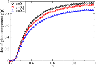
Figure 1: Size of giant component $g(p)$ in single networks with degree distribution Eq. (9) and average degree $\langle k\rangle=4$, as a function of $p$, the fraction of remaining nodes after random removal of nodes. Curves are from theory Eq. 10, symbols are from simulation.

This equation is a closed-form solution for the giant component $g(p)$ and can be solved numerically. The critical case appears when the derivatives of the both sides of Eq. (10) are equal. That leads to the critical condition $\langle k\rangle p_{c}=1$, which is independent of clustering. However the degree distribution of the doubly Poisson model changes as we keep the average degree and change the clustering coefficient. When the degree distribution is fixed, the critical threshold actually increases as clustering increases  [29, 30]. Furthermore, Fig. 1 shows the resulting giant component as a function of $p$. Note that single networks with higher clustering have smaller giant components.

3 Degree-Degree Correlation

When constructing clustering in a network, it is usually impossible to avoid generating degree-degree correlations. To better understand the effect of clustering on degree-degree correlations, we present an analytical expression of degree correlation as a function of the clustering coefficient for a doubly Poisson-clustered network—see Eq. (9).

The degree-degree correlation [32] can be expressed as

$$\rho_{D}=\frac{N_{1}N_{3}-N_{2}^{2}}{N_{1}\sum\limits_{i=1}^{N}d_{i}^{3}N_{2}^{2}}$$ (11)

where $N_{m}$ is the total number of $m$ hop walks between all possible node pairs $(i,j)$ including cases $i=j$.

The generating function of the degree of a node in the network is $\sum\limits_{s,t=0}^{\infty}P_{st}z^{s+2t}=G_{0}(z,z^{2})$. Let $q_{st}$ be the fraction of nodes with $s$ single edges and $t$ triangles that are reached by traversing a random single link, where $s$ includes the traversed link and $r_{st}$ is the fraction of nodes with $s$ single edges and $t$ triangles reached by traversing a link of a triangle, $q_{st}=\frac{sP_{s,t}}{\langle s\rangle},r_{st}=\frac{tP_{s,t}}{\langle t\rangle}$. Their corresponding generating functions are $G_{q}(x,y)=\frac{1}{\langle s\rangle}\frac{\partial G_{0}(x,y)}{\partial x}x$ and $G_{r}(x,y)=\frac{1}{\langle t\rangle}\frac{\partial G_{0}(x,y)}{\partial y}y$. Moreover, $N_{3}=\sum\limits_{i}\sum\limits_{j}a_{ij}N_{2}(j)$, where $N_{2}(j)$ is the total number of two-hop walks starting from node $j$. The number of three-hop walks from a node $i$ is equal to the total number of two-hop walks starting from all of its neighbors. Thus, $N_{3}=\sum\limits_{j}k_{j}N_{2}(j)$, where the number of two-hop walks starting from a node $j$ with degree $k_{j}$ will be counted $k_{j}$ times in $N_{3}$. Equivalently, $N_{3}=N\sum\limits_{st}(s+2t)P_{s,t}N_{2}(s,t)$, where $N_{2}(s,t)$ is the number of two hop walks from a node with $s$ single edges and $t$ triangles. The generating function of the number of single edges and of triangles reached in two hops from a random node is $G_{2}(x,y)=\sum\limits_{st}P_{s,t}\cdot G_{q}^{s}(x,y)\cdot G_{r}^{2t}(x,y)$. The generating function of the total number of links and of triangles reached within three hops starting from all nodes is $G_{3}(x,y)=N\sum\limits_{st}P_{s,t}\cdot\left(G_{q}(x,y)\right)^{s(s+2t)}\cdot\left(G_{r}(x,y)\right)^{2t(s+2t)}$. The number $N_{k}$ of $k$-hop walks can be approximated by its mean in a large network

$$N_{1} = N\langle k\rangle,$$

$$N_{2} = N\frac{\partial G_{2}}{\partial x}\left|x=1,y=1\right.+2N\frac{\partial G_{2}}{\partial y}\left|x=1,y=1\right.$$

$$N_{3} = \frac{\partial G_{3}}{\partial x}\left|x=1,y=1\right.+2\frac{\partial G_{3}}{\partial y}\left|x=1,y=1\right.$$

When both $s$ and $t$ follow a Poisson distribution,

$$G_{0}(x,y) = e^{\mu(x-1)}e^{\nu(y-1)}$$

$$G_{q}(x,y) = G_{0}(x,y)x$$

$$G_{r}(x,y) = G_{0}(x,y)y.$$

In this case,

$$N_{1} = N\langle k\rangle$$

$$N_{2} = N\left\langle k\right\rangle\left(\frac{\left\langle k\right\rangle}{1-c}+1\right)$$

$$N_{3} = \left(\langle k\rangle^{3}+2\langle k\rangle^{2}+4\nu\langle k\rangle+\langle k\rangle+6\nu\right)N\text{ }$$

$$\sum\limits_{i=1}^{N}d_{i}^{3} = \left(\left\langle k\right\rangle^{3}+3\left\langle k\right\rangle^{2}+(6\nu+1)\left\langle k\right\rangle+6\nu\right)N,$$

which together with Eq. (11) leads to

$$\rho_{D}=\frac{c-c^{2}-\langle k\rangle c^{2}}{1-c+\langle k\rangle c-2\langle k\rangle c^{2}},$$ (12)

where c is the clustering coefficient, Eq. (3).

Figure 2 shows the relation between the degree correlation and the clustering coefficient $c$ for a Poissonian network [see Eq. (9)], for two given average degrees ($\langle k\rangle=3$ and 4). The figure shows a positive degree-degree correlation across the entire range, which means the model is assortative [29]. The degree-degree correlation increases until $c$ achieves half of its maximum and then decreases to zero when $c$ reaches its maximum. When $c$ is 0 or the maximum, the nodes connect to either all single links or all triangles, respectively.

4 Percolation on Interdependent Clustered Networks

To study how clustering within interdependent networks affects a system’s robustness, we apply the interdependent networks framework [17]. In interdependent networks A and B, a fraction $(1-p)$ of nodes is first removed from network A. Then the size of the giant components of networks A and B in each cascading failure step is defined to be $p_{1}$, $p_{2}$, …, $p_{n}$, which are calculated iteratively

$$\begin{array}[]{l}p_{n}=\mu_{n-1}g_{A}(\mu_{n-1}),\mbox{n is odd,}\\ p_{n}=\mu_{n}g_{B}(\mu_{n}),\mbox{n is even,}\end{array}$$ (13)

where $\mu_{0}=p$ and $\mu_{n}$ are intermediate variables that satisfy

$$\begin{array}[]{l}\mu_{n}=pg_{A}(\mu_{n-1}),\mbox{n is odd,}\\ \mu_{n}=pg_{B}(\mu_{n-1}),\mbox{n is even.}\end{array}$$ (14)

As interdependent networks A and B form a stable mutually-connected giant component, $n\rightarrow\infty$ and $\mu_{n}=\mu_{n-2}$, the fraction of nodes left in the giant component is $p_{\infty}$. This system satisfies

$$\begin{array}[]{l}x=pg_{A}(y),\\ y=pg_{B}(x),\end{array}$$ (15)

where the two unknown variables $x$ and $y$ can be used to calculate $p_{\infty}=xg_{B}(x)=yg_{A}(y)$. Eliminating $y$ from these equations, we obtain a single equation

$$x=pg_{A}[pg_{B}(x)].$$ (16)

The critical case ($p=p_{c}$) emerges when both sides of this equation have equal derivatives,

$$1=p^{2}\frac{dg_{A}}{dx}[pg_{B}(x)]\frac{dg_{B}}{dx}(x)|_{x=x_{c},p=p_{c}},$$ (17)

which, together with Eq. (16), yields the solution for $p_{c}$ and the critical size of the giant mutually-connected component, $p_{\infty}(p_{c})=x_{c}g_{B}(x_{c})$.

Consider for example the case in which each network has doubly-Poisson degree distributions as in Eq. (9). From Eq. (15), we have $x=p(1-u_{A})$, $y=p(1-u_{B})$, where

$$\begin{array}[]{l}u_{A}=v_{A}=e^{[\mu_{A}y+2y(1-y)\mu_{A}](u_{A}-1)+\nu_{A}p^{2}(v_{A}^{2}-1)},\\ u_{B}=v_{B}=e^{[\mu_{B}x+2x(1-x)\mu_{B}](u_{B}-1)+\nu_{B}p^{2}(v_{B}^{2}-1)}.\\ \end{array}$$

If the two networks have the same clustering, $\mu\equiv\mu_{A}=\mu_{B}$ and $\nu\equiv\nu_{A}=\nu_{B}$, $p_{\infty}$ is then

$$p_{\infty}=p(1-e^{\nu p_{\infty}^{2}-(\mu+2\nu)p_{\infty}})^{2}.$$ (18)

The giant component, $p_{\infty}$, for interdependent clustered networks can thus be obtained by solving Eq. (18). Note that when $\nu=0$ we obtain from Eq. (18) the result obtained in Ref. [17] for random interdependent ER networks. Figure 3a, using numerical simulation, compares the size of the giant component after $n$ stages of cascading failure with the theoretical prediction of Eq. (13). When $p=0.7$ and $p=0.64$, which are not near the critical threshold ($p_{c}=0.6609$), the agreement with simulation is perfect. Below and near the critical threshold, the simulation initially agrees with the theoretical prediction but then deviates for large $n$ due to the random fluctuations of structure in different realizations [17]. By solving Eq. (18), we have $p_{\infty}$ as a function of $p$ in Fig. 3b for a given average degree and several values of clustering coefficients and in Fig. 4a for a given clustering and for different average degree values. As the figure shows, when higher clustering within a network is introduced, the percolation transition yields a higher value of $p_{c}$ (see inset of Fig. 3b).

When clustering changes in this doubly Poisson distribution model, degree distribution and degree-degree correlation also change. First, to address the influence of the degree distribution, we study the critical thresholds of shuffled clustered networks. Shuffled clustered networks have neither clustering nor degree-degree distribution but keep the same degree distribution as the original clustered networks. The brown dashed curve in Fig. 3b represents the giant component of interdependent shuffled clustered networks with original clustering $c=0.2$. The figure shows that the difference in $p_{c}$ between the $c=0$ network and the shuffled $c=0.2$ network is only $0.01$, while the difference between the $c=0$ and the $c=0.2$ networks is $0.12$. In addtion, $c=0.2$ clustered networks has no degree-degree correlation (Fig. 2), which means the $0.12$ shift of $p_{c}$ is due to clustering and not to a change in degree distribution. We also show the critical thresholds of interdependent shuffled clustered networks as the red dashed line in the inset of Fig. 3b. Note that the change of degree distribution barely shifts the critical threshold. We next discuss the effect of the degree-degree correlation on the change of critical threshold. From Ref. [34], the degree assortativity alone monotonously [??? JDM] increases the percolation critical threshold of interdependent networks. Because in our case degree-degree correlation first increases and then decreases (see Fig. 2), while critical the threshold of interdependent networks increases monotonously [???] as clustering increases, we conclude that clustering alone increases the value of $p_{c}$. Thus clustering within networks reduces the robustness of interdependent networks. This probably occurs because clustered networks contain some links in triangles that do not contribute to the giant component, and in each stage of cascading failure the giant component will be smaller than in the unclustered case.

We also study the effect of the mean degree $\langle k\rangle$ on the percolation critical point. Figures 4a and 4b both show that, when clustering is fixed, the percolation critical point of interdependent networks decreases as the average degree $\langle k\rangle$ of network increases, making the system more robust. Figure 4b also shows that a larger minimum average degree is needed to maintain the network against collapse without any node removal as clustering increases.

5 Conclusion and Summary

To conclude, based on Newman’s single network clustering model, we present a generating-function formalism solution for site percolation on both single and interdependent clustered networks. We also derive an analytical expression, Eq. (12), for degree-degree correlation as a function of the clustering coefficient for a doubly-Poisson network. Our results help us better understand the effect of clustering on the percolation of interdependent networks. We discuss the influence of a change of degree distribution and the degree-degree correlation associated with clustering in the model on the critical threshold of interdependent networks and conclude that $p_{c}$ for interdependent networks increases when networks are more highly clustered.

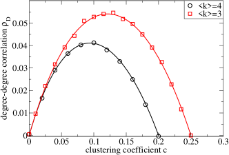
Figure 2: Degree-degrees correlation as a function of the clustering coefficient for Poisson network (Eq. (9)) with average degree $\langle k\rangle=3$ and 4. Curves are from theory (Eq. 12) and symbols from simulations.

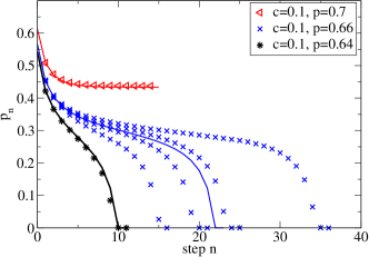
(a)

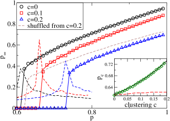
(b)

Figure 3: (a) Size of mutually connected giant component as a function of cascading failure steps $n$. Results are for $c=1$, $p=0.64$ (below $p_{c}$), $p=0.66$ (at $p_{c}$) and $p=0.7$ (above $p_{c}$). Lines represent theory (Eqs. (13) and (14)) and dots are from simulations. Note that at $p_{c}$ there are large fluctuations. (b) Size of giant component, $p_{\infty}$, in interdependent networks with both networks having clustering via degree distribution Eq. (9) and average degree $\langle k\rangle=4$, as a function of $p$. Dashed lines are number of interactions (NOI) before cascading failure stops obtained by simulation [33]. The star curve is for shuffled $c=0.2$ network, which keeps the same degree distribution but without clustering and without degree-degree correlation. Inset: Green squares and solid line represents critical thresholds, $p_{c}$, of interdependent networks as a function of clustering coefficient $c$. Red dashed line represents critical threshold of shuffled interdependent networks which originally has clustering coefficient $c$. The shuffled networks have zero clustering and degree-degree correlation, but has the same degree distribution as the original clustered networks. In all figures, symbols and dashed lines represent simulation, solid curves represent theoretical results.

(a)

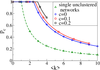
(b)

Figure 4: (a) Size of giant component as a function of $p$ for fixed clustering coefficient $c=0.1$ and different average degrees. From right to left $\langle k\rangle=3,4,5,...,9$. (b) Critical threshold $p_{c}$ as a function of average degree for different clustering coefficients. The solid curves are for interdependent networks and the dashed curve is for single networks. Symbols and curves represent simulation and theoretical predictions respectively.

- [1] Rosato V., et al. Int. J. Crit. Infrastruct. 4 (2008) 63.
- [2] US-Canada Power System Outage Task Force: Final report on the August 14th 2003 Blackout in the United States and Canada, (The Task Force, 2004).
- [3] Peerenboom J., Fischer R., and Whitefield R., Proc. CRIS/DRM/IIIT/NSF Workshop Mitigating the Vulnerability of critical Infrastructures to Catastrophic Failures (2001).
- [4] Rinaldi S., Peerenboomand J., and Kelly T., IEEE Control. Syst. Magn. 21 (2001) 11.
- [5] Yagan O., Qian D., Zhang J., and Cochran D., Special Issue of IEEE Transactions on Parallel and Distributed Systems (TPDS) on Cyber-Physical Systems (2012).
- [6] Vespignani A., Nature (London) 464 (2010) 984.
- [7] Zimmerman R., 2004 IEEE Int. Conf. Syst. Man Cybern. 5 (2005) 4059.
- [8] Mendonca D. and Wallace W., J. Infrast. Syst. 12 (2006) 260.
- [9] Robert B., Morabito L., and Christie R. D., Int. J. Crit. Infrastruct. 4 (2008) 353.
- [10] Reed D. A., Kapur K. C., and Christie R. D., IEEE Syst. J. 3 (2009) 174.
- [11] E. Bagheri and Ghorbani A. A., Inform. Syst. Front. 12 (2009) 115.
- [12] Mansson D., Thottappillil R., Backstrom M., and Ludvika H. V. V., IEEE Trans. Electromagn. Compat. 95 (2009) 46.
- [13] Johansson J. and Hassel H., Reliab. Eng. Syst. Saf. 95 (2010) 1335.
- [14] Bashan A., et al., Nature Communication 3, (2012) 702.
- [15] Li W., et al., Phys. Rev. Lett 108, (2012) 228702.
- [16] Bashan A., et al., arXiv:1206.2062, (2012).
- [17] Buldyrev S. V., et al. Nature (London) 464 (2010) 1025.
- [18] Parshani R., et al. Phys. Rev. Lett. 105 (2010) 048701.
- [19] Huang X., Gao J., Buldyrev S. V., Havlin S., and Stanley H. E., Phys. Rev. E (R) 83 (2011) 065101.
- [20] Shao J., Buldyrev S. V., Havlin S., and Stanley H. E., Phys. Rev. E 83 (2011) 036116.
- [21] Gao J., Buldyrev S. V., Stanley H. E., and Havlin S., Nature Physics 8 (2011) 40.
- [22] Gao J., Buldyrev S. V., Havlin S., and Stanley H. E., Phys. Rev. Lett. 107 (2011) 195701.
- [23] Watts D. J. and Strogatz S. H., Nature (London) 393 (1998) 440.
- [24] Newman M. E. J. and Park J., Phys. Rev. E 68 (2003) 036122.
- [25] Serrano M. A. and Boguñá M., Phys. Rev. E 74 (2006) 056114.
- [26] Newman M. E. J., Phys. Rev. Lett. 103 (2009) 058701.
- [27] Miller J. C., Phys. Rev. E 80 (2009) 020901(R).
- [28] Gleeson J. P., Phys. Rev. E 80 (2009) 036107.
- [29] Gleeson J. P., S. Melnik, and A. Hackett, Phys. Rev. E 81 (2010) 066114.
- [30] A. Hackett, S. Melnik, and Gleeson J. P., Phys. Rev. E 83 (2011) 056107.
- [31] Molina C. and Stone L. doi: 10.1016/j.jtbi.2012.08.036.
- [32] Van Mieghem P., Wang H., Ge X., Tang S., and Kuipers F. A., Eur. Phys. J. B 76 (2010) 643.
- [33] Parshani R. et al., Proc. Natl. Acad. Sci. USA 108 (2011) 1007.
- [34] Zhou D., D’Agostino G., Scala A., and Stanley H. E., arXiv:1203.0029v1 (2012).