The SL2S Galaxy-scale Gravitational Lens Sample. I. The alignment of mass and light in massive early-type galaxies at $z=0.2-0.9$

Abstract

We study the relative alignment of mass and light in a sample of 16 massive early-type galaxies at $z=0.2-0.9$ that act as strong gravitational lenses. The sample was identified from deep multi-band images obtained as part of the Canada France Hawaii Telescope Legacy Survey as part of the Strong Lensing Legacy Survey (SL2S). Higher resolution follow-up imaging is available for a subset of 10 systems. We construct gravitational lens models and infer total enclosed mass, elongation, and position angle of the mass distribution. By comparison with the observed distribution of light we infer that there is a substantial amount of external shear with mean value $\langle\gamma_{\rm ext}\rangle=0.12\pm 0.05$, arising most likely from the environment of the SL2S lenses. In a companion paper, we combine these measurements with follow-up Keck spectroscopy to study the evolution of the stellar and dark matter content of early-type galaxies as a function of cosmic time.

1. Introduction

The last two decades have seen the emergence of a hierarchical model for the formation of structure in the universe. The main ingredients, dominating the overall dynamics of the universe, are non-relativistic particles that do not interact with light or baryons except through gravity (i.e., cold dark matter), and the mysterious dark energy (Perlmutter et al. 1999; Riess et al. 1998), i.e., a term in the stress-energy tensor of the universe characterized by negative pressure (or equivalently a cosmological constant).

The familiar standard model particles move and interact with each other within this skeleton of unknown particles and fields (White & Rees 1978). Although standard model particles represent only a small minority of the total energy budget of the universe (Komatsu et al. 2011), they play a crucial role in the formation of galaxies, and their constituents stars and planets. In those overdense regions of the universe, interactions between standard model particles alter their dynamics and spatial distribution. Indirectly, through gravitational interactions, this so-called baryonic physics in turn modifies the properties of the underlying dark matter distribution (Blumenthal et al. 1986; Gnedin et al. 2004; Duffy et al. 2010). Understanding the interplay between baryons and dark matter at sub-galactic scales is crucial not only for any effort to understand how galaxies form and evolve, but also may shed light on the properties of the dark matter itself (e.g., self-interaction cross-section; Spergel & Steinhardt 2000; Loeb & Weiner 2011).

From an observational point of view, it is very challenging to measure accurately the relative distribution of baryonic and dark matter on sub-galactic scales. By-and-large, traditional methods require the presence of a luminous tracer (e.g., hot plasma, cold gas, or stars), whose kinematics are then interpreted to reconstruct the underlying gravitational potential (e.g., Saglia et al. 1992; Gerhard et al. 2001; Humphrey et al. 2006; Franx et al. 1994). Gravitational lensing (especially strong lensing at sub-galactic scales; Treu 2010) provides an additional and powerful tool to shed light on dark matter. By exploiting the deflection of light rays from background sources it need not rely on the presence of luminous tracers in the deflector. Furthermore, gravitational lensing is only sensitive to the total gravitational potential and therefore can provide accurate measurements of mass and mass distribution independent of its dynamical state or nature.

The combination of strong gravitational lensing with other diagnostic tools, such as stellar kinematics (e.g., Miralda-Escude 1995; Natarajan & Kneib 1996; Treu & Koopmans 2002, 2004; Koopmans & Treu 2003; Sand et al. 2004; Gavazzi 2005; Koopmans et al. 2006, 2009b; Grillo et al. 2008; Czoske et al. 2008, 2012; Barnabè et al. 2009b, a, 2011; Sonnenfeld et al. 2012), weak lensing (Gavazzi et al. 2007; Lagattuta et al. 2010; Auger et al. 2010), stellar populations synthesis methods (e.g., Grillo et al. 2009; Auger et al. 2009, 2010; Thomas et al. 2011; Tortora et al. 2010; Treu et al. 2010; Spiniello et al. 2011, 2012), etc., is particularly effective. By breaking a number of degeneracies inherent to each method alone one can give precise answers to a number of questions. What is the relative abundance of dark and luminous matter in the inner parts of galaxies? Are dark matter density profiles universal as those predicted by simulations? Are halos as triaxial as predicted by simulations? How much of the dark matter observed in galaxies is baryonic (i.e., low-mass stars and high-mass stars remnants) and how much is non-baryonic?

Until a few years ago, answers to these questions based on strong gravitational lensing where mostly limited by the small samples of known lenses. In fact, strong lensing is a relatively rare phenomenon, and in general only $\sim 1/1000$ background galaxy will have a massive foreground deflector sufficiently well aligned along the line of sight to produce multiple images (e.g., Turner et al. 1984; Schneider et al. 1992; Chae 2003). However, this situation is changing rapidly owing to the dedicated efforts of a number of groups in exploiting massive imaging and spectroscopic surveys such as the Sloan Lens ACS Survey (SLACS), the Boss Emission Lines Lens Survey (BELLS), the HST Archive Galaxy-scale Gravitational Lens Survey, or the Strong Lensing Legacy Survey (SL2S) to find samples of strong lenses (Browne et al. 2003; Bolton et al. 2006; Marshall et al. 2009; Treu et al. 2011; Brownstein et al. 2012). In the past few years, dedicated searches using a variety of techniques and wavelengths have delivered well over 200 galaxy-scale strong lenses.

1.1. The Strong Lensing Legacy Survey

The SL2S (Cabanac et al. 2007) is a dedicated effort to find strong lens systems in the Canada-France-Hawaii Telescope Legacy Survey (CFHTLS) with the goal of answering fundamental questions about the distribution of mass and light. It consists of two main efforts: the group and cluster-scale survey (Limousin et al. 2009; More et al. 2012; Verdugo et al. 2011) and this present series that is concerned with the follow-up and analysis of the galaxy-scale sample (R. Gavazzi et al., in preparation).

The candidates are identified using the RingFinder algorithm which detects compact rings around centers of isolated galaxies ($\lesssim 10^{13}M_{\sun}$), and works by looking for blue features in excess of an early-type galaxies (ETGs) smooth light distribution that are consistent with the presence of lensed arcs. After selecting a sample of bright ($i_{\rm AB}\leq 22.5$) red galaxies in the redshift range $0.1\leq z\leq 0.8$, a scaled, Point Spread Function (PSF) matched version of the $i$-band image was subtracted from the $g$-band image. The rescaling in this operation is performed such that the ETG light is efficiently removed, leaving only objects with a spectral energy distribution different from that of the target galaxy. These typically blue residuals are then characterized with an object detector, and analyzed for their position, ellipticity, and orientation, and those with properties consistent with lensed arcs are kept as lens candidates. In practice, we require the blue excess to be elongated (axis ratio $b/a<1/2$) and tangentially aligned ($\pm 25^{\circ}$) with respect to the center of the foreground potential deflector. We also consider favorably multiple residual objects with similar colors. The objects are searched for within an annulus of inner and outer radius $0\farcs 5$ and $2\farcs 7$, respectively. The lower bound is chosen to discard fake residual coming from the unresolved inner structure of the deflector, inaccurate PSFs, etc. The outer bound is chosen to limit the detection of the many singly imaged objects that only experience a modest amount of shear (see, R. Gavazzi et al., in preparation, for further details). A sample of several hundred good candidates was visually inspected and ranked for follow-up Hubble Space Telescope (HST) imaging and Very Large Telescope (VLT) or Keck spectroscopy. These observations are required to confirm the actual lensing nature of the systems and to allow accurate lens modeling. In practice, our selection process finds about 2-3 lens candidates per square degree. Extensive follow-up shows that the sample is 50%-60% pure (see, R. Gavazzi et al., in preparation). The SL2S galaxy-scale sample provides an ideal higher-$z$ complement to the SLACS: the deflectors have similar distribution in size and velocity dispersion, but they have a median redshift of $\sim 0.5$ (cf. $z_{d}\sim 0.2$ for SLACS), extending the baseline for evolutionary studies back to two thirds of the current age of the universe.

In this series we construct lens models for a pilot sample of confirmed SL2S galaxy-scale lenses for which Keck spectroscopy is available, and interpret them by themselves and in combination with stellar kinematics and stellar population synthesis models (Paper II; Ruff et al. 2011). This first paper presents lens models for 16 confirmed systems as well as one candidate which proved impossible to model with simple gravitational potentials and was therefore discarded as a strong lens. We use the results of the lens modeling to discuss relative orientation of mass and light and their flattening. Following the approach of many lens surveys before us (e.g., Bolton et al. 2006, 2008b; Treu et al. 2006; Koopmans et al. 2006), we carry out this pilot analysis using standard but relatively simple models, in order to provide an initial benchmark and to illustrate the quality of the data and the potential of the survey. Specifically, the models presented here are based on singular isothermal elliptical potentials and simply parameterized sources. Using the Einstein radii presented here, the companion Paper II discusses the relative abundance of mass and light and the evolution of the mass density profile by combining the SL2S, SLACS, and Lens Structure and Dynamics (LSD) samples. We are currently working to enlarge the sample substantially and gather more follow-up data. Future papers of this series will present the enlarged sample as well as more sophisticated lens models designed to exploit the richer dataset and sample size.

This paper is organized as follows. In Section 2 we introduce the CFHT and HST data used in the analysis. In Section 3 we describe our modeling techniques. Section 4 describes the lens models and presents our results on the relative alignment of mass and light. A brief discussion of the properties of the lensed sources is also presented. Section 5 concludes with a brief summary.

Throughout this paper magnitudes are given in the AB system. We assume a concordance cosmology with matter and dark energy density $\Omega_{m}=0.3$, $\Omega_{\Lambda}=0.7$, and Hubble constant $H_{0}$=70 km s^-1Mpc^-1.

2. Observations

2.1. CFHT Data

The CFHTLS consists of two main components of sufficient depth and image quality to be interesting for lens searches. Both are imaged in the $u^{*}$, $g$, $r$, $i$ and $z$ bands with the 1 deg² field-of-view Megacam Camera. The multi epoch Deep Survey covers four pointing of 1 deg² each. Two different image stacks were produced: D-85 contains the 85% best seeing images whereas the D-25 only includes the 25% best seeing images. For finding lenses we only considered the better resolution stacks. In the T06 data release (Goranova et al. 2009) used for this study they reach a typical depth of $u^{*}\simeq 26.18$, $g=\simeq 25.96$, $r\simeq 25.43$, $i\simeq 25.08$, and $z\simeq 24.57$ (80% completeness for point sources) with typical FWHM PSFs of $0\farcs 75$, $0\farcs 69$, $0\farcs 64$, $0\farcs 62$ and $0\farcs 61$, respectively. The Wide survey is a single epoch imaging survey, covering approximately 171 deg² in 4 patches of the sky. It reaches a typical depth of $\rm u^{*}\simeq 25.35$, $\rm g\simeq 25.47$, $\rm r\simeq 24.83$, $\rm i\simeq 24.48$, and $\rm z\simeq 23.60$ (AB mag of 80% completeness limit for point sources) with typical FWHM PSFs of $0\farcs 85$, $0\farcs 79$, $0\farcs 71$, $0\farcs 64$ and $0\farcs 68$, respectively. Owing to the greater survey solid angle, the Wide component is our main source of lens candidates.

Around each candidate lens and in each CFHTLS band, we produce cutout images 101 pixels (i.e.  $18\farcs 8$) wide. Nearby stars within 5 arcmin from a given lens are used to produce a PSF model. The 17 systems analyzed in this study are shown in Figures 1-4 and listed in Table 2.

2.2. HST Follow-up Imaging

In order to confirm the lensing hypothesis and allow for detailed lens modeling, 65 galaxy-scale lens candidates have been observed with the HST as snapshot programs during cycles 15, 16, 17 (GOs 10876, 11289, PI: J.-P. Kneib; GO 11588, PI: R. Gavazzi). The observations started with the Advanced Camera for Surveys (ACS), then switched to the Wide Field and Planetary Camera 2 (WFPC2) after the failure of ACS, and finally turned to the Wide Field Camera 3 (WFC3) after Servicing Mission 4. Approximately, 50% of the lens candidates were confirmed as lenses in this way. A more comprehensive description of the efficiency of the SL2S lens finding strategy will be given by R. Gavazzi et al. (in preparation).

Ten of the galaxy-scale systems were observed with HST early enough to be included in our first Keck spectroscopic follow-up campaign and are the subject of papers I and II. The remaining systems will be presented at the end of our Keck and HST observing campaigns in the next papers of this series. Of these ten systems, three were observed in two bands, with ACS or WFC3 whereas the others were observed only in a single WFPC2 band as detailed in Table 1.

All the WFPC2 data were reduced using standard MultiDrizzle recipes. The cosmic ray removal worked well because the 1200 s exposure time was split into three exposures. The “drizzling” was performed by preserving the CCD frame orientation and pixel scale to avoid producing correlated noise. The ACS and WFC3 observations consisted of single or double exposures only and therefore we relied on LA-Cosmic (van Dokkum 2001) on individual exposures for cosmic ray removal, before combining them with swarp (Bertin et al. 2002). As for WFPC2, images are kept in the natural CCD frame. Exposure times and final pixel scales are given in Table 1.

Table 1 Summary of HST observations.

name	instrument/filter	exp. time	pixel scale
		(sec)	(arcsec)
SL2SJ021411$-$040502	ACS/F606W	400	0.05
	ACS/F814W	800	0.05
SL2SJ021737$-$051329	ACS/F606W	400	0.05
	ACS/F814W	800	0.05
SL2SJ022511$-$045433	WFPC2/F606W	1200	0.1
SL2SJ022610$-$042011	WFPC2/F606W	1200	0.1
SL2SJ022648$-$040610	WFPC2/F606W	1200	0.1
SL2SJ023251$-$040823	WFPC2/F606W	1200	0.1
SL2SJ140123$+$555705	WFPC2/F606W	1200	0.1
SL2SJ141137$+$565119	WFC3/F475X	720	0.04
	WFC3/F600LP	720	0.04
SL2SJ221326$-$000946	WFPC2/F606W	1200	0.1
SL2SJ221407$-$180712	WFPC2/F606W	1200	0.1

3. Modeling methodology

In order to model the light distribution of a galaxy-scale gravitational lens, one has to disentangle the contribution of the foreground deflector and that of the background lensed arc-like features. The former is generally a red ETG and the former a dimmer, blue, and presumably star-forming, more distant source. The light distribution of an ETG generally has a regular shape sufficiently well described by a Sérsic (Sersic 1968) or even a de Vaucouleurs profile (de Vaucouleurs 1948) with very small color gradients. Blue background sources are also well represented by Exponential profiles (Newton et al. 2011). The separation of these two components is relatively straightforward for ETGs deflectors and they can generally be fitted independently for most applications. However, very detailed investigations of the source properties of high signal-to-noise data might require a simultaneous fit of both components (e.g., Marshall et al. 2007), especially with ground-based data (F. Brault et al., in preparation) and bright arcs. We describe our procedure to fit the foreground deflector in Section 3.1. In Section 3.2 we describe how we use the residual lensed images to model the gravitational potential of the deflector and the intrinsic surface brightness of the source.

3.1. Foreground Deflector

We used the versatile galfit software (Peng et al. 2002) to perform the subtraction of the foreground deflector as it allows to account for boxyness/diskyness of isophotes. It generally yields good image subtraction with a Sérsic profile (see Figure 1) but the recovered Sérsic indices $n$ and effective radii $R_{\rm eff}$ are quite degenerate.

We thus used a generic Sérsic profile with more degrees of freedom to get as good a deflector subtraction as possible and we also applied a strong $n=4$ prior to get a more precise value of $R_{\rm eff}$. In the same vein, the fit of the $n=4$ foreground lens also yields a robust measurement of ellipticity and orientation of the light distribution. These values are reported in Table 2.

Fits are performed in all the available bands of a given lens using $18\farcs 8$ on a side cutout images and suitable PSF either inferred from the neighboring stars or from TinyTim (Krist et al. 2011) in the case of HST data. The formal errors on each parameter are generally very small because they only account for statistical errors and not modeling errors associated with the mismatches between the form of the assumed and observed light distribution. A more realistic estimate of the total uncertainties on the recovered ellipticity, orientation and effective radius can be made by estimating the filter-to-filter dispersion on these parameters when HST data are missing. When HST imaging is available, shape parameters characterizing the deflector are more robustly measured and we adopt the formal errors from galfit.

3.2. Lensed Features and Mass Modeling

For lens modeling we used a dedicated code sl_fit developed for and tested on galaxy-scale strong lenses (e.g., Gavazzi et al. 2007, 2008, 2011; Tu et al. 2009). The code fits model parameters of simple analytic lensing potentials. It uses the full surface brightness distribution observed in the image plane and attempts to explain it with one or more simple analytic light components described by an exponential radial profile with elliptical shape (see, e.g., Marshall et al. 2007; Bolton et al. 2008a; Newton et al. 2011, for similar techniques).

The lensing potential is assumed to be made of a singular isothermal ellipsoid (SIE), centered on the main deflector. This is the simplest mass profile that has been shown to yield a description of the mass distribution of massive ETGs sufficient to derive Einstein radius, position angle, and ellipticity (e.g., Rusin et al. 2003; Rusin & Kochanek 2005; Koopmans et al. 2006; Gavazzi et al. 2007; Koopmans et al. 2009a; Barnabè et al. 2011). The convergence profile of the central mass component is given by

$$\kappa(x,y)=\frac{b}{2\xi},$$ (1)

where the scaling parameter $b$ is the Einstein radius $R_{\rm Ein}$ (e.g., Schneider et al. 1992; Kormann et al. 1994). $b$ is related to the velocity dispersion of the deflector through $b/1\arcsec=(\sigma_{v}/186.21\,\,{\rm km\,s}^{-1})^{2}D_{\rm ls}/D_{\rm s}$, where $D_{\rm ls}$ and $D_{\rm s}$ are angular diameter distance between the lens and the source and between the observer and the source, respectively. $\xi^{2}=qx^{2}+y^{2}/q$ is the radial coordinate that accounts for the ellipsoidal symmetry of the isodensity contours and $q$ is the minor-to-major axis ratio. The orientation of the major axis P.A._tot is allowed to vary, although this is not explicit in the definition of Equation (1). We do not assume a priori that the orientation of the total mass distribution is correlated to that of the observed stellar component. In this way, the total potential can capture (and mix because of substantial degeneracies) internal and external quadrupolar terms in the potential (Keeton et al. 1997). We also add an external shear parameter when more information is available (see the case of SL2SJ021737$-$051329 described below), sufficient to break the degeneracy between external shear and orientation of the galaxy potential.

As in the previous step, when we fitted the foreground light distribution, we weigh pixels with the image inverse total variance (including sky, foreground, and lensed features). The $\chi^{2}$ term relating the observed light distribution $I(\mathbf{x}_{i})$ at pixel $i$ and the intrinsic source light distribution $S(\mathbf{y})$ is thus:

$$\chi^{2}=\sum_{i}\frac{\left[I(\mathbf{x}_{i})-S(\mathbf{x}_{i}-\boldsymbol{\alpha}(\mathbf{x_{i}}|\mathbf{p}_{\rm p})|\mathbf{p}_{s})\right]^{2}}{\sigma_{i}^{2}}\;,$$ (2)

where $\mathbf{p}_{\rm p}=[b,q,{\rm P.A.}_{\rm SIE}]$ contains the parameters that determine the gravitational potential and $\mathbf{p}_{s}=[x_{\rm s},y_{\rm s},q_{\rm s},{\rm P.A.}_{\rm s},m_{\rm s},r_{\rm s}]$ is the section of the parameter space that describes the source light distribution, namely, its center $\mathbf{x}_{s}$, its ellipticity $q_{\rm s}$, its orientation P.A._s, its magnitude $m_{\rm s}$, and half-light radius $r_{\rm s}$.

The optimization of these nine parameters is performed using Monte Carlo Markov Chain techniques. Reported model parameters and confidence intervals are taken from the 0.50, 0.16, and 0.84 quantiles. However, because of the simplicity of both the model potential and model source light distribution, we generally end up with very small formal errors on the recovered model parameters that should be substantially increased. Bolton et al. (2008a) estimated that relative errors on $R_{\rm Ein}$ should be about 5%. We thus add this dominant contribution in quadrature to the statistical errors in Table 2 and do the same for the axis ratio $q_{\rm SIE}$ by adding a $\pm 0.07$ absolute error on consistent with Newton et al. (2011) and even more conservative than the $\pm 0.05$ error quoted by Bolton et al. (2008a).

4. Results

In this section we describe the lens model of each system (Section 4.1). In addition, we study the shape and relative orientation of the light and total mass distributions as they do are independent of the source and deflector redshift (Section 4.2). Results depending on spectroscopic information (source and deflector redshifts and velocity dispersion) along with a novel method proposed to mitigate the nuisance due to the ignorance of the source redshift are presented in Paper II.

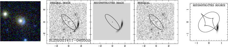
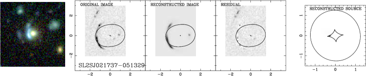
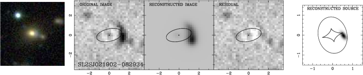
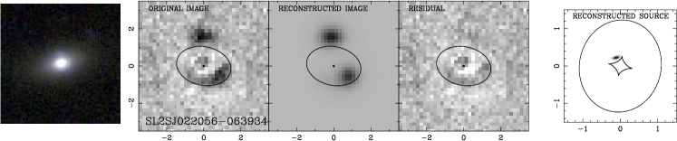
Figure 1.— Results of the lens modeling analysis. For each row, a system is shown with, from left to right, a $18\farcs 8\times 18\farcs 8$ CFHTLS gri composite image of the system, the lensed features with the deflector subtracted off with galfit (data), the best-fit model prediction (model), the residual (data$-$model) and the associated source plane light distribution. The critical lines are overlaid in the first three panels whereas the caustics lines are shown in the last one.

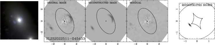
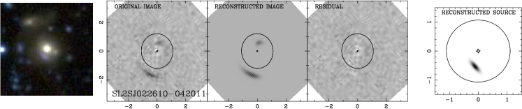
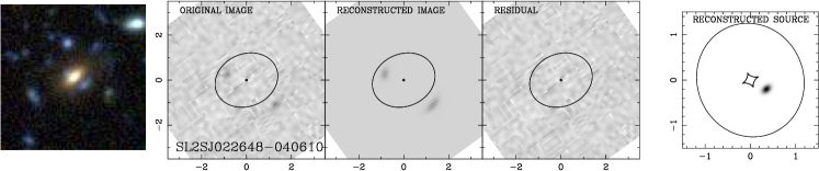
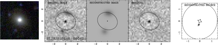
Figure 2.— Lens models (continued).

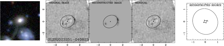
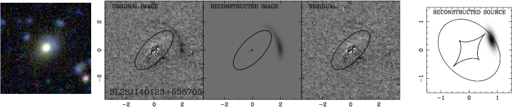
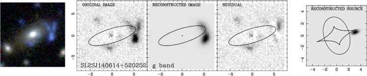
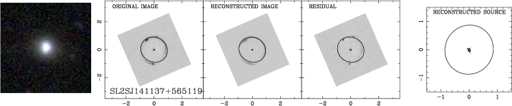
Figure 3.— Lens models (continued). Note the different plotting range for the third row corresponding to SL2SJ140614+520252.

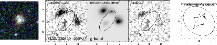
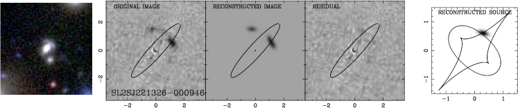
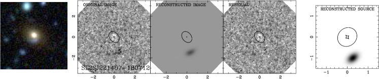
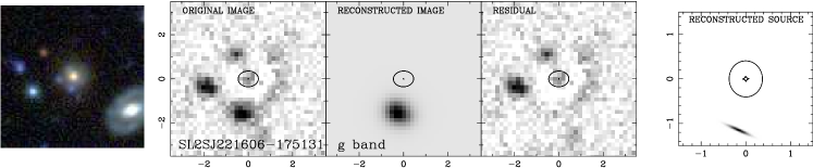
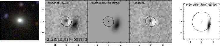
Figure 4.— Lens models (continued). Note that the system in the third row, SL2SJ221606-175131, is not a satisfying model of a lens and we disqualify it as being an actual gravitational lens.

4.1. Notes on Individual Lens Models

For each lens in the sample we describe the resulting best-fit model.

• SL2SJ021411$-$040502 can be reproduced by a single SIE potential + Exponential source model, located just outside the caustic. We note a small axis ratio $q_{\rm SIE}\sim 0.33$ this seems at odds with the more circular light distribution $q_{*}\sim 0.89$. This can be explained by the presence of a neighbor galaxy at the same redshift as $z_{\rm d}$ about 8″and ${\rm P.A.}\sim 65^{\circ}$ which enhances the elongation of the potential. An alternative solution with a slightly lower likelihood is found where the source is located just inside the caustic and the lensing configuration consists of three merging images (one of which is barely visible in the HST image). This solution has a larger Einstein radius (by $\sim$30%), a slightly rounder potential, and a different position angle (elongation almost east–west). For the present study we adopt the solution with the highest likelihood although the secondary solution cannot be excluded completely without deeper HST data.

• SL2SJ021737$-$051329 has been studied by in detail by Tu et al. (2009). Our results are in agreement with theirs. A simple SIE + Exponential source yields a good fit, even though a better fit is achieved by introducing both internal ellipticity through the SIE potential and external shear (consistent with the presence of a nearby group of galaxies). Similar conclusions were recently found by Cooray et al. (2011) using additional near-IR CANDELS data. The source redshift is $z_{\rm s}=1.847$ (Paper II). This implies that the source half-light radius is $R_{\rm eff,s}=0\farcs 081^{+0.028}_{-0.016}\simeq 0.69^{+0.24}_{-0.13}\,{\rm kpc}$ for an F606W magnitude $m_{\rm s}=24.45\pm 0.10$. The system is lensing a second source at $z_{s2}\sim 2.3$ that we do not consider here for consistency with the other systems. However, regardless of whether the second source is modeled or not, the good signal-to-noise ratio and the favorable image configuration allows us to break the degeneracy between external shear and internal ellipticity and we therefore get constraints on both. We find an external shear $\gamma_{\rm ext}=0.064\pm 0.003$ with an orientation P.A.${}_{\rm ext}=89\fdg 7\pm 0\fdg 4$. We see that the light is well aligned with the external shear and about $\sim 33\deg$ misaligned with the SIE component. The SIE mass component is found to have a rather circular distribution ($q_{\rm SIE}=0.91\pm 0.07$, Table 2), we thus do not consider this apparently strange behavior too seriously as some of the mass ellipticity (internal quadrupole) could be exchanged with external shear with a slightly different mass profile (Tu et al. 2009).

• SL2SJ021902$-$082934 is another ”cusp” configuration with a marginal candidate counter image on the opposite side. The lack of HST imaging implies that we had to consider the CFHT $g$-band image. We can see an additional source westward of the arc that has a color similar of the deflector and should not be considered as a lensed feature. Since we can achieve a good fit of the arc without introducing this perturbation we neglect it.

• SL2SJ022056$-$063934 is a minor axis cusp configuration. The single source component does not perfectly capture the faint tail of the inner arc although most of the flux is well recovered, even with ground-based resolution.

• SL2SJ022511$-$045433 is a low-redshift bright deflector with another bright minor axis cups configuration. The source redshift is $z_{\rm s}=1.199$ (Paper II). We report here the result with a single source component of magnitude $m_{s}=24.14\pm 0.04$ in the F606W band and half-light radius $R_{\rm eff,s}=0\farcs 125\pm 0\farcs 003\simeq 1.037\pm 0.025\,{\rm kpc}$. Note that we also attempted to account for the fainter extension of the furthest arc (on the east of the deflector), with a secondary component. This would even lower the residuals on the two multiple images without changing the results on the recovered potential parameters. Accounting for this component the source would be $\sim 0.36$ mag brighter.

• SL2SJ022610$-$042011 is a typical large impact parameter double configuration implying a substantial differential magnification of the two multiple images. In addition, these two are nearly aligned with the center of the deflector. This is consistent with the potential being close to circularly symmetric ($q_{\rm SIE}\sim 0.92$). This system has a known source redshift $z_{\rm s}=1.232$. We can thus estimate the source half-light radius $R_{\rm eff,s}=0\farcs 160\pm 0\farcs 011\simeq 1.332\pm 0.092\,{\rm kpc}$ for an F606W magnitude $m_{\rm s}=25.10\pm 0.08$.

• SL2SJ022648$-$040610 is another double configuration with a more balanced magnification ratio between the two images involving a slightly more elongated potential. We note that the deflector looks like an edge-on S0 galaxy with an elongated light distribution. However, the total potential is considerably more circular.

• SL2SJ022648$-$090421 is also modeled using Megacam $g$ band data and shows a minor axis cusp configuration with little deviation between light and SIE orientations. This is the faintest source we reconstruct with $m_{\rm s}=27.13\pm 0.14$.

• SL2SJ023251$-$040823 is a double system with the source close to the cusp.

• SL2SJ140123+555705 shows a dim cusp-like arc. Even though we cannot identify the counterimage, the substantial bending of the arc breaks the degeneracy between shear and intrinsic source ellipticity and allows us to measure the Einstein radius with good accuracy $R_{\rm Ein}=1\farcs 19\pm 0\farcs 07$, comparable to the other cases.

• SL2SJ140614+520252 is another cusp configuration on a larger scale, as $R_{\rm Ein}=3\farcs 02\pm 0\farcs 15$. Some blue light excesses are seen in the $g$-band image shown in Figure 3 and only the main “naked” cusp arc is captured by our model. However, we can see that the other western component is not multiply imaged as the source would fall outside the caustic. Thus, it does not provide more information and we verified that its inclusion does not change our conclusions on the lensing potential. Even by ignoring this second singly imaged source component, we find that this system involves the brightest source of the sample with $g$ band $m_{\rm s}=23.50\pm 0.03$. We could not find a solution with a lensed source reproducing the southern and northeastern blue excesses. The lens potential is highly elongated with $q_{\rm SIE}=0.290\pm 0.015$. This is probably due to the additional contribution of a nearby galaxy about $8\farcs 3$ in the southeast direction that corresponds to the major axis of the already quite elongated light component.

• SL2SJ141137+565119 is the only system having WFC3 imaging presented here. The signal-to-noise ratio is good and allows us to get tight constraints on the potential and on the source whose redshift is found to be $z_{\rm s}=1.420$. The source half-light radius in the F475X band is $R_{\rm eff,s}=0\farcs 0.058\pm 0\farcs 001\simeq 0.490\pm 0.008\,{\rm kpc}$ and its magnitude is $m_{\rm s}=25.86\pm 0.04$. We note that the addition of a very compact core would improve the fit further as our single source component does not reproduce the full complexity of the source light distribution. Our best-fit model nevertheless captures most of the extended Einstein ring.

• SL2SJ220629+005728 is modeled using the $g$-band Megacam image. However, we see in the color cutout image that a small red satellite lies on top of the lensed blue features. We thus need to disentangle both contributions by simultaneously fitting to the $g$ and $i$ bands one lensed source and one foreground unlensed source centered in the red satellite. This satellite also contributes to the lens potential through a point mass component of unknown mass. We find that this perturbing mass has to be $M_{\rm pert}\leq 2\times 10^{9}\,M_{\odot}$ (68% CL). Getting HST imaging data would significantly improve the accuracy of the decomposition and the constraints on $M_{\rm pert}$. The Einstein radius estimate is robust with respect to the inclusion (or not) of the perturbing potential.

• SL2SJ221326$-$000946 is an edge-on disk galaxy in which both the potential and the light distribution are highly elongated: $q_{\rm SIE}=0.191\pm 0.014$ and $q_{*}=0.277\pm 0.007$ with a small $\Delta{\rm P.A.}\sim 10\fdg 4\pm 0\fdg 6$ misalignment.

• SL2SJ221407$-$180712 does not exhibit any counterimage nor a strong curvature of the main outer image. This implies that the model cannot be constrained well and we can only place upper limits on the Einstein radius $R_{\rm Ein}=0\farcs 41\pm 0\farcs 23$. The results on the potential elongation and orientation are thus very loose and we do not consider this system in the statistical analysis of Section 4.2. Note that the small upper limit on $R_{\rm Ein}$ is consistent with other mass constraints in Paper II.

• SL2SJ221606$-$175131 has a relatively symmetric configuration. Its similarity to a classic quad configuration lead us to include it in the lens candidate sample. However, we could not find any sensible lens model able to reproduce in detail the image configuration. Therefore we cannot conclude that this system is a lens, or more precisely, that the blue features about 1$\arcsec$ from the center of the ETG originate from a unique background source. We speculate that it could be due to low surface brightness star formation at the ETG’s redshift. We thus exclude this system from the statistical analysis below, although better imaging data would be useful to revisit this system by constructing more complex models of the source and potential.

• SL2SJ221929$-$001743 does not have HST imaging and the CFHT data do not allow us to constraint tightly the potential parameters as we cannot identify unambiguously a counterimage. In addition, the arc does not display a strong curvature at the resolution of ground-based imaging. We thus get weaker constraints on the Einstein radius $R_{\rm Ein}=0\farcs 74\pm 0\farcs 14$ than for other systems. HST imaging would significantly improve the mass model. Given the redshift of the source $z_{\rm s}=1.023$, we infer a source half-light radius $R_{\rm eff,s}=0\farcs 384^{+0.073}_{-0.054}\simeq 3.03^{+0.59}_{-0.43}\,{\rm kpc}$ and a $g$ band intrinsic magnitude $m_{\rm s}=24.08\pm 0.21$.

4.2. Alignment of Mass and Light

The top panel of Figure 5 compares the ellipticity of the stellar component to that of the mass model. For the vast majority of the objects the ellipticities are tightly correlated. This is expected since stellar mass makes up a significant fraction of the total mass within the Einstein radius. However, there are few interesting outliers. The flattened light distribution of SL2SJ022648$-$040610 is consistent with a disky galaxy living in significantly rounder halo. Perhaps more surprising are the cases of SL2SJ021411$-$040502 and SL2SJ220629+005728, where the stars are almost round, while the potential is significantly flattened. In both cases the source of the ellipticity of the mass distribution seems to be external shear, associated with a satellite. In general, the relation between light and mass ellipticity seems to have significantly more scatter than that found for the SLACS sample, $\langle q_{\rm SIE}/q_{*}\rangle=0.95$ with scatter 0.48, as opposed to 0.99 with scatter 0.11 (Koopmans et al. 2006). As we discuss in the next paragraph this is probably due to a much more significant role played by external shear.

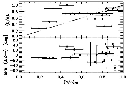
Figure 5.— Top panel: correlation between axis ratio of the light and of the mass distribution. Bottom panel: angular offset between the major axis of the mass distribution and that of the light as a function of axis ratio of the mass distribution. SL2SJ021737$-$051329 is not included because this system was modeled including external shear.

The bottom panel of Figure 5 shows the angular offset between light and mass P.A. as a function of mass ellipticity. Even neglecting the points with $q_{\rm SIE}>0.85$, where clearly the position angle is not very well measured since the potential is so circular, there is considerable scatter around zero. For the entire sample the rms scatter is 25 deg, while if we limit ourselves to $q_{\rm SIE}<0.85$ the scatter is still 18 deg. Again this is considerable higher than the 10 deg found for the SLACS sample (Koopmans et al. 2006) in general, and closer to the values found for the subset of SLACS lenses that reside in overdense environments (Treu et al. 2009). A simple calculation, based on Equation (22) in the paper by Keeton et al. (1997) and assuming that the direction of external shear is randomly distributed with respect to that of the mass of the galaxies shows that this is consistent with a relatively large average external shear. This is illustrated in Figure 6 where we show the expected rms fluctuation of the position angles as a function of average external shear. Regardless of whether the rounder objects are included or not, it seems that external shear $\langle\gamma_{\rm ext}\rangle=0.12\pm 0.05$ is required on average. The mean and error on this quantity are estimated by propagating the sampling variance associated with the measurement of the $\pm 25^{\circ}$ rms dispersion in the light-mass misalignment angle. The small sample size prevents us from further estimations like the scatter about this mean value which, in turn, will be addressed in a forthcoming paper (Sonnenfeld et al., in preparation). This level of external shear is fairly common among galaxy-scale gravitational lenses (e.g., Keeton et al. 1997; Holder & Schechter 2003), and it is likely due to the environment of the lenses (Auger et al. 2007; Treu et al. 2009; Auger 2008; Wong et al. 2011), since massive ETGs typically reside at the centers of groups. The lower level of external shear in the SLACS sample, $\langle\gamma_{\rm ext}\rangle\lesssim 0.035$ (Koopmans et al. 2006), is most likely due to the smaller size of their Einstein radius relative to the characteristic scale of the galaxy (half effective radius typically), and therefore the more relevant role played by stellar mass in defining the potential within the critical curve. It is also possible that part of the observed misalignments between the light and the gravitational potential might arising from intrinsic misalignments between the galaxy and its halo. This is also expected to be a larger effect in SL2S than in SLACS, owing to the larger size of the Einstein radius relative to the effective radius. We will explore this issue further in future papers of this series with a larger sample and better data.

Finally, we also note that, despite the likely greater influence of the environment relative to SLACS, the SL2S lenses do not require as large a quadrupolar term as CLASS radio source or quasars (Keeton et al. 1997). This might be due to the fact that extended sources are not as sensitive to the magnification bias that would boost the fraction of highly magnified quads. In turn, the only unambiguous quad systems here are J141137+565119 and J021737$-$051329. Two out of 16 lenses (excluding J221606$-$175131) are quads.

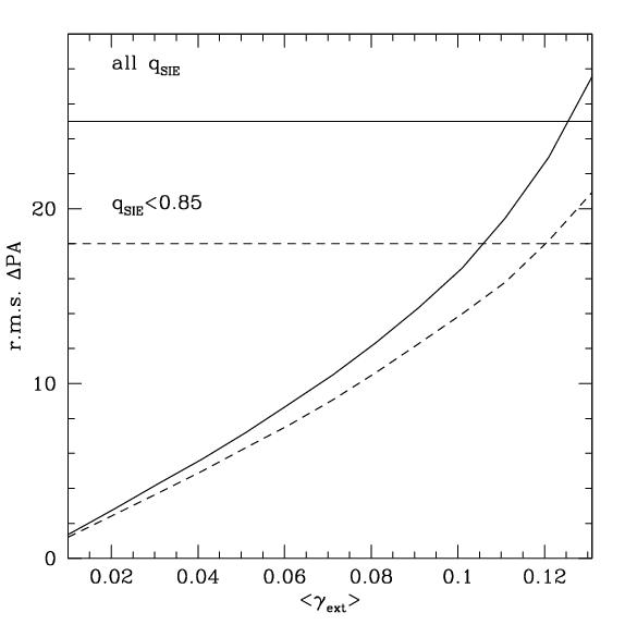
Figure 6.— The curves represent the expected rms fluctuations of the offset in P.A. as a function of average external shear. The horizontal lines represent the values measured for the SL2S sample. The solid lines refer to the whole sample, while the dashed lines refer to the subsample with mass axis ratio $q_{\rm SIE}<0.85$.

5. Summary

In this paper we presented gravitational lens models of a pilot sample of 16 galaxy-scale lenses identified as part of the SL2S Survey. HST imaging is available for 10/16 systems, while for the others the modeling is based on ground-based CFHTLS imaging. After removing the light from the foreground deflector we used the surface brightness distribution of the background source to constrain mass models of the deflector galaxy. For each system we derived Einstein radius, position angle, and ellipticity of the mass distribution described as a SIE. These parameters are used in Paper II in combination with spectroscopic information to study the relative distribution of stellar and dark matter in ETGs and its evolution with cosmic time. In this paper we focused on the relative orientation and ellipticity of the luminous and total mass distribution, which does not require spectroscopic information. We found that the ellipticity of mass and light are correlated except for three outliers. In one case the presence of a disk makes the light distribution significantly flatter than the overall mass distribution. In two cases, the presence of a nearby galaxy introduces significant external shear in the overall mass distribution. In addition, we found that the position angle of mass and light is on average aligned, albeit with rms scatter of 18-25 deg, significantly larger than what is found for the lower redshift SLAC sample. We interpreted this scatter as most likely due to substantial external shear, on average $\langle\gamma_{\rm ext}\rangle=0.12\pm 0.05$, resulting from the environment (physically related to the main deflector galaxy or along the line of sight). The physical scale of the SL2S Einstein radii is greater that for SLACS: $R_{\rm Ein}/R_{\rm eff}\simeq 1.1$ versus 0.5 for SLACS (Auger et al. 2010). In addition, we found only two quad lenses in this pilot sample, suggesting that magnification bias is less effective in boosting the statistics of extended lensed sources as compared with samples comprising point sources.

In Paper II we combine our lensing information with stellar kinematics to infer the cosmic evolution of the mass density profile of massive galaxies. Given the sample size in these first two papers of the series, the role of environment and external shear cannot be explored further, neither in terms of astrophysical signal, nor in terms of systematic uncertainty on the mass density slope. However, the follow-up imaging and spectroscopy of SL2S candidates are still ongoing and we plan to investigate these issues with a much larger sample in future papers of this series. The parallel effort of measuring the redshift of sources with Keck and XShooter on VLT will also allow us to explore the population of lensed sources with greater detail.

Table 2Summary of key observables.

name	$z_{\rm d}$	$m_{i}$	input	$R_{\rm Eff}$	$R_{\rm Ein}$	$q_{\rm SIE}$	P.A.SIE	$q_{\rm*}$	P.A.∗	source mag
		(AB)		(arcsec)	(arcsec)
SL2SJ021411$-$040502	0.609	18.78	ACS/F606W	$0.94\pm 0.05$	$0.92\pm 0.07$	$0.33\pm 0.08$	$42.3\pm 1.3$	$0.89\pm 0.02$	$53.6\pm 4.0$	$24.30\pm 0.12$
SL2SJ021737$-$051329	0.646	19.47	ACS/F606W	$0.77\pm 0.04$	$1.27\pm 0.06$	$0.91\pm 0.07$	$124.3\pm 2.4$	$0.92\pm 0.02$	$91.2\pm 4.5$	$24.45\pm 0.10$
SL2SJ021902$-$082934	0.390	19.33	Megacam/g	$0.90\pm 0.08$	$0.92\pm 0.06$	$0.53\pm 0.09$	$102.0\pm 4.1$	$0.73\pm 0.01$	$79.7\pm 1.0$	$25.35\pm 0.19$
SL2SJ022056$-$063934	0.330	18.35	Megacam/g	$1.47\pm 0.04$	$1.25\pm 0.06$	$0.73\pm 0.07$	$76.6\pm 2.1$	$0.57\pm 0.01$	$105.0\pm 0.5$	$25.74\pm 0.09$
SL2SJ022511$-$045433	0.238	16.84	WFPC2/F606W	$1.90\pm 0.09$	$1.77\pm 0.09$	$0.58\pm 0.07$	$26.3\pm 0.2$	$0.75\pm 0.01$	$26.0\pm 0.7$	$24.14\pm 0.04$
SL2SJ022610$-$042011	0.494	18.78	WFPC2/F606W	$0.56\pm 0.03$	$1.15\pm 0.06$	$0.92\pm 0.08$	$5.3\pm 10.9$	$0.83\pm 0.01$	$56.2\pm 1.2$	$25.10\pm 0.08$
SL2SJ022648$-$040610	0.766	20.01	WFPC2/F606W	$1.20\pm 0.06$	$1.31\pm 0.07$	$0.82\pm 0.07$	$112.1\pm 5.2$	$0.34\pm 0.01$	$131.8\pm 0.6$	$26.17\pm 0.09$
SL2SJ022648$-$090421	0.456	18.32	Megacam/g	$1.30\pm 0.04$	$1.58\pm 0.09$	$0.83\pm 0.08$	$68.1\pm 4.2$	$0.81\pm 0.01$	$61.6\pm 0.9$	$27.13\pm 0.14$
SL2SJ023251$-$040823	0.352	18.58	WFPC2/F606W	$0.81\pm 0.04$	$1.10\pm 0.06$	$0.80\pm 0.07$	$122.0\pm 0.8$	$0.68\pm 0.01$	$110.2\pm 0.8$	$26.39\pm 0.08$
SL2SJ140123$+$555705	0.526	19.14	WFPC2/F606W	$0.76\pm 0.04$	$1.19\pm 0.07$	$0.49\pm 0.08$	$126.7\pm 6.5$	$0.73\pm 0.01$	$136.0\pm 1.1$	$25.19\pm 0.17$
SL2SJ140614$+$520252	0.480	18.29	Megacam/g	$2.15\pm 0.16$	$3.02\pm 0.15$	$0.29\pm 0.07$	$107.2\pm 0.1$	$0.48\pm 0.01$	$120.4\pm 0.6$	$23.50\pm 0.03$
SL2SJ141137$+$565119	0.322	18.49	WFC3/F475X	$0.76\pm 0.04$	$0.92\pm 0.05$	$0.90\pm 0.07$	$61.4\pm 0.3$	$0.88\pm 0.01$	$17.7\pm 1.4$	$25.86\pm 0.04$
SL2SJ220629$+$005728	0.704	20.59	Megacam/g	$2.25\pm 0.24$	$1.34\pm 0.07$	$0.46\pm 0.07$	$143.3\pm 0.2$	$0.99\pm 0.02$	$108.8\pm 5.1$	$25.81\pm 0.08$
SL2SJ221326$-$000946	0.338	20.00	WFPC2/F606W	$0.41\pm 0.02$	$1.08\pm 0.05$	$0.19\pm 0.07$	$138.0\pm 0.5$	$0.28\pm 0.01$	$148.4\pm 0.6$	$25.14\pm 0.04$
SL2SJ221407$-$180712	0.650	20.43	WFPC2/F606W	$0.57\pm 0.03$	$0.41\pm 0.23$	$0.69\pm 0.16$	$62.3\pm 46.9$	$0.73\pm 0.01$	$57.5\pm 0.8$	$25.29\pm 0.32$
SL2SJ221606$-$175131	0.860	20.68	Megacam/g	$0.93\pm 0.08$	–	–	–	$0.87\pm 0.01$	$57.4\pm 3.1$	$25.67\pm 0.07$
SL2SJ221929$-$001743	0.289	17.78	Megacam/g	$1.00\pm 0.03$	$0.74\pm 0.14$	$0.75\pm 0.16$	$85.3\pm 35.5$	$0.74\pm 0.01$	$84.3\pm 0.6$	$24.08\pm 0.21$

Note. — Effective radii and associated errors are estimated from the mean and standard deviation of a galfit de Vaucouleurs fit in each of the $r$, $i$, and $z$ Megacam bands when HST imaging is not available. When one or more HST bands are available, $R_{\rm eff}$ is measured on the reddest one (See table 1) but the error is still obtained from the Megacam bands. (a) As discussed in Section 4.1, we could not model SL2SJ221606$-$175131 as a lens and therefore do not report lensing parameters for this system.

References

- Auger (2008) Auger, M. W. 2008, MNRAS, 383, L40
- Auger et al. (2007) Auger, M. W., Fassnacht, C. D., Abrahamse, A. L., Lubin, L. M., & Squires, G. K. 2007, AJ, 134, 668
- Auger et al. (2009) Auger, M. W., Treu, T., Bolton, A. S., et al. 2009, ApJ, 705, 1099
- Auger et al. (2010) Auger, M. W., Treu, T., Bolton, A. S., et al. 2010, ApJ, 724, 511
- Barnabè et al. (2011) Barnabè, M., Czoske, O., Koopmans, L. V. E., Treu, T., & Bolton, A. S. 2011, MNRAS, 415, 2215
- Barnabè et al. (2009a) Barnabè, M., Czoske, O., Koopmans, L. V. E., et al. 2009a, MNRAS, 399, 21
- Barnabè et al. (2009b) Barnabè, M., Nipoti, C., Koopmans, L. V. E., Vegetti, S., & Ciotti, L. 2009b, MNRAS, 393, 1114
- Bertin et al. (2002) Bertin, E., Mellier, Y., Radovich, M., et al. 2002, in Astronomical Society of the Pacific Conference Series, Vol. 281, Astronomical Data Analysis Software and Systems XI, ed. D. A. Bohlender, D. Durand, & T. H. Handley, 228
- Blumenthal et al. (1986) Blumenthal, G. R., Faber, S. M., Flores, R., & Primack, J. R. 1986, ApJ, 301, 27
- Bolton et al. (2008a) Bolton, A. S., Burles, S., Koopmans, L. V. E., et al. 2008a, ApJ, 682, 964
- Bolton et al. (2006) Bolton, A. S., Burles, S., Koopmans, L. V. E., Treu, T., & Moustakas, L. A. 2006, ApJ, 638, 703
- Bolton et al. (2008b) Bolton, A. S., Treu, T., Koopmans, L. V. E., et al. 2008b, ApJ, 684, 248
- Browne et al. (2003) Browne, I. W. A. et al. 2003, MNRAS, 341, 13
- Brownstein et al. (2012) Brownstein, J. R., Bolton, A. S., Schlegel, D. J., et al. 2012, ApJ, 744, 41
- Cabanac et al. (2007) Cabanac, R. A., Alard, C., Dantel-Fort, M., et al. 2007, A&A, 461, 813
- Chae (2003) Chae, K. 2003, MNRAS, 346, 746
- Cooray et al. (2011) Cooray, A., Fu, H., Calanog, J., et al. 2011, ArXiv e-prints: 1110.3784
- Czoske et al. (2008) Czoske, O., Barnabè, M., Koopmans, L. V. E., Treu, T., & Bolton, A. S. 2008, MNRAS, 384, 987
- Czoske et al. (2012) Czoske, O., Barnabè, M., Koopmans, L. V. E., Treu, T., & Bolton, A. S. 2012, MNRAS, 419, 656
- de Vaucouleurs (1948) de Vaucouleurs, G. 1948, Annales d’Astrophysique, 11, 247
- Duffy et al. (2010) Duffy, A. R., Schaye, J., Kay, S. T., et al. 2010, MNRAS, 405, 2161
- Franx et al. (1994) Franx, M., van Gorkom, J. H., & de Zeeuw, T. 1994, ApJ, 436, 642
- Gavazzi (2005) Gavazzi, R. 2005, A&A, 443, 793
- Gavazzi et al. (2011) Gavazzi, R., Cooray, A., Conley, A., et al. 2011, ApJ, 738, 125
- Gavazzi et al. (2008) Gavazzi, R., Treu, T., Koopmans, L. V. E., et al. 2008, ApJ, 677, 1046
- Gavazzi et al. (2007) Gavazzi, R., Treu, T., Rhodes, J. D., et al. 2007, ApJ, 667, 176
- Gerhard et al. (2001) Gerhard, O., Kronawitter, A., Saglia, R. P., & Bender, R. 2001, AJ, 121, 1936
- Gnedin et al. (2004) Gnedin, O. Y., Kravtsov, A. V., Klypin, A. A., & Nagai, D. 2004, ApJ, 616, 16
- Goranova et al. (2009) Goranova, Y., Hudelot, P., Magnard, F., et al. 2009, The CFHTLS T0006 Release, Tech. rep., Terapix – Institut d’Astrophysique de Paris, http://terapix.iap.fr/cplt/T0006/T0006-doc.pdf
- Grillo et al. (2009) Grillo, C., Gobat, R., Lombardi, M., & Rosati, P. 2009, A&A, 501, 461
- Grillo et al. (2008) Grillo, C., Gobat, R., Rosati, P., & Lombardi, M. 2008, A&A, 477, L25
- Holder & Schechter (2003) Holder, G. P. & Schechter, P. L. 2003, ApJ, 589, 688
- Humphrey et al. (2006) Humphrey, P. J., Buote, D. A., Gastaldello, F., et al. 2006, ApJ, 646, 899
- Keeton et al. (1997) Keeton, C. R., Kochanek, C. S., & Seljak, U. 1997, ApJ, 482, 604
- Koekemoer et al. (2002) Koekemoer, A. M., Fruchter, A. S., Hook, R. N., & Hack, W. 2002, in The 2002 HST Calibration Workshop : Hubble after the Installation of the ACS and the NICMOS Cooling System, ed. S. Arribas, A. Koekemoer, & B. Whitmore, p337
- Komatsu et al. (2011) Komatsu, E., Smith, K. M., Dunkley, J., et al. 2011, ApJS, 192, 18
- Koopmans et al. (2009a) Koopmans, L. V. E., Barnabe, M., Bolton, A., et al. 2009a, Astronomy, 2010, 159
- Koopmans et al. (2009b) Koopmans, L. V. E., Bolton, A., Treu, T., et al. 2009b, ApJ, 703, L51
- Koopmans & Treu (2003) Koopmans, L. V. E. & Treu, T. 2003, ApJ, 583, 606
- Koopmans et al. (2006) Koopmans, L. V. E., Treu, T., Bolton, A. S., Burles, S., & Moustakas, L. A. 2006, ApJ, 649, 599
- Kormann et al. (1994) Kormann, R., Schneider, P., & Bartelmann, M. 1994, A&A, 284, 285
- Krist et al. (2011 ) Krist, J. E., Hook, R. N., & Stoehr, F. 2011 in (SPIE, Optical Modeling and Performance Predictions V), 81270J
- Lagattuta et al. (2010) Lagattuta, D. J., Fassnacht, C. D., Auger, M. W., et al. 2010, ApJ, 716, 1579
- Limousin et al. (2009) Limousin, M., Cabanac, R., Gavazzi, R., et al. 2009, A&A, 502, 445
- Loeb & Weiner (2011) Loeb, A. & Weiner, N. 2011, Physical Review Letters, 106, 171302
- Marshall et al. (2009) Marshall, P. J., Hogg, D. W., Moustakas, L. A., et al. 2009, ApJ, 694, 924
- Marshall et al. (2007) Marshall, P. J. et al. 2007, ApJ, 671, 1196
- Miralda-Escude (1995) Miralda-Escude, J. 1995, ApJ, 438, 514
- More et al. (2012) More, A., Cabanac, R., More, S., et al. 2012, ApJ, 749, 38
- Natarajan & Kneib (1996) Natarajan, P. & Kneib, J.-P. 1996, MNRAS, 283, 1031
- Newton et al. (2011) Newton, E. R., Marshall, P. J., Treu, T., et al. 2011, ApJ, 734, 104
- Peng et al. (2002) Peng, C. Y., Ho, L. C., Impey, C. D., & Rix, H.-W. 2002, AJ, 124, 266
- Perlmutter et al. (1999) Perlmutter, S., Aldering, G., Goldhaber, G., et al. 1999, ApJ, 517, 565
- Riess et al. (1998) Riess, A. G., Filippenko, A. V., Challis, P., et al. 1998, AJ, 116, 1009
- Ruff et al. (2011) Ruff, A. J., Gavazzi, R., Marshall, P. J., et al. 2011, ApJ, 727, 96
- Rusin & Kochanek (2005) Rusin, D. & Kochanek, C. S. 2005, ApJ, 623, 666
- Rusin et al. (2003) Rusin, D., Kochanek, C. S., & Keeton, C. R. 2003, ApJ, 595, 29
- Saglia et al. (1992) Saglia, R. P., Bertin, G., & Stiavelli, M. 1992, ApJ, 384, 433
- Sand et al. (2004) Sand, D. J., Treu, T., Smith, G. P., & Ellis, R. S. 2004, ApJ, 604, 88
- Schneider et al. (1992) Schneider, P., Ehlers, J., & Falco, E. E. 1992, Gravitational Lenses (Springer-Verlag Berlin Heidelberg New York)
- Sersic (1968) Sersic, J. L. 1968, Atlas de galaxias australes (Cordoba, Argentina: Observatorio Astronomico)
- Sonnenfeld et al. (2012) Sonnenfeld, A., Treu, T., Gavazzi, R., et al. 2012, ApJ, 752, 163
- Spergel & Steinhardt (2000) Spergel, D. N. & Steinhardt, P. J. 2000, Physical Review Letters, 84, 3760
- Spiniello et al. (2011) Spiniello, C., Koopmans, L. V. E., Trager, S. C., Czoske, O., & Treu, T. 2011, MNRAS, 417, 3000
- Spiniello et al. (2012) Spiniello, C., Trager, S. C., Koopmans, L. V. E., & Chen, Y. P. 2012, ApJ, 753, L32
- Thomas et al. (2011) Thomas, J., Saglia, R. P., Bender, R., et al. 2011, MNRAS, 415, 545
- Tortora et al. (2010) Tortora, C., Napolitano, N. R., Romanowsky, A. J., & Jetzer, P. 2010, ApJ, 721, L1
- Treu (2010) Treu, T. 2010, ARA&A, 48, 87
- Treu et al. (2010) Treu, T., Auger, M. W., Koopmans, L. V. E., et al. 2010, ApJ, 709, 1195
- Treu et al. (2011) Treu, T., Dutton, A. A., Auger, M. W., et al. 2011, MNRAS, 417, 1601
- Treu et al. (2009) Treu, T., Gavazzi, R., Gorecki, A., et al. 2009, ApJ, 690, 670
- Treu et al. (2006) Treu, T., Koopmans, L. V., Bolton, A. S., Burles, S., & Moustakas, L. A. 2006, ApJ, 640, 662
- Treu & Koopmans (2002) Treu, T. & Koopmans, L. V. E. 2002, ApJ, 575, 87
- Treu & Koopmans (2004) Treu, T. & Koopmans, L. V. E. 2004, ApJ, 611, 739
- Tu et al. (2009) Tu, H., Gavazzi, R., Limousin, M., et al. 2009, A&A, 501, 475
- Turner et al. (1984) Turner, E. L., Ostriker, J. P., & Gott, III, J. R. 1984, ApJ, 284, 1
- van Dokkum (2001) van Dokkum, P. G. 2001, PASP, 113, 1420
- Verdugo et al. (2011) Verdugo, T., Motta, V., Muñoz, R. P., et al. 2011, A&A, 527, A124
- White & Rees (1978) White, S. D. M. & Rees, M. J. 1978, MNRAS, 183, 341
- Wong et al. (2011) Wong, K. C., Keeton, C. R., Williams, K. A., Momcheva, I. G., & Zabludoff, A. I. 2011, ApJ, 726, 84