Subsampling at Information Theoretically Optimal Rates

Abstract

We study the problem of sampling a random signal with sparse support in frequency domain. Shannon famously considered a scheme that instantaneously samples the signal at equispaced times. He proved that the signal can be reconstructed as long as the sampling rate exceeds twice the bandwidth (Nyquist rate). Candès, Romberg, Tao introduced a scheme that acquires instantaneous samples of the signal at random times. They proved that the signal can be uniquely and efficiently reconstructed, provided the sampling rate exceeds the frequency support of the signal, times logarithmic factors.

In this paper we consider a probabilistic model for the signal, and a sampling scheme inspired by the idea of spatial coupling in coding theory. Namely, we propose to acquire non-instantaneous samples at random times. Mathematically, this is implemented by acquiring a small random subset of Gabor coefficients. We show empirically that this scheme achieves correct reconstruction as soon as the sampling rate exceeds the frequency support of the signal, thus reaching the information theoretic limit.

I Introduction

I-A Definitions

For the sake of simplicity, we consider a discrete-time model (analogous to the one of [4]) and denote signals in time domain as $x\in{\mathbb{C}}^{n}$, $x=(x(t))_{1\leq t\leq n}=(x(1),\dots,x(n))^{\sf T}$. Their discrete Fourier transform is denoted by $\widehat{x}\in{\mathbb{C}}^{n}$, $\widehat{x}=(\widehat{x}(\omega))_{\omega\in\Omega_{n}}$, where $\Omega_{n}=\{\omega=2\pi k/n:k\in\{0,1,\dots,\\ n-1\}\}$. The Fourier transform $\widehat{x}=({\sf F}x)$ is given by

$$\widehat{x}(\omega)=\langle b_{\omega},x\rangle=\sum_{t=1}^{n}\overline{b_{\omega}(t)}\;x(t)\,,\quad b_{\omega}(t)\equiv\frac{1}{\sqrt{n}}\,e^{i\omega t}\,.$$ (1)

Here $\langle\,\cdot\,,\,\cdot\,\rangle$ denotes the standard scalar product on ${\mathbb{C}}^{n}$. Also, for a complex variable $z$, $\overline{z}$ is the complex conjugate of $z$. Notice that $(b_{\omega})_{\omega\in\Omega_{n}}$ is an orthonormal basis of ${\mathbb{C}}^{n}$. This implies Parseval’s identity $\langle\widehat{x}_{1},\widehat{x}_{2}\rangle=\langle x_{1},x_{2}\rangle$. In addition, the inverse transform is given by

$$x(t)=\sum_{\omega\in\Omega_{n}}\widehat{x}(\omega)\,b_{\omega}(t)=\frac{1}{\sqrt{n}}\sum_{\omega\in\Omega_{n}}\widehat{x}(\omega)\,e^{i\omega t}\,.$$ (2)

We will denote by $T_{n}=\{1,\dots,n\}$ the time domain, and will consider signals that are sparse in the Fourier domain.

A sampling mechanism is defined by a measurement matrix $A\in{\mathbb{R}}^{m\times n}$. Measurement vector $y=(y(1),\dots,y(m))^{\sf T}\in{\mathbb{R}}^{m}$ is given by

$$y=Ax+w\equiv y_{0}+w\,,$$ (3)

where $w$ is a noise vector with variance $\sigma^{2}$, and $y_{0}$ is the vector of ideal (noiseless) measurements. In other words, $y(i)=\langle a_{i},x\rangle$ where we let $a_{1}^{*},\dots a_{m}^{*}$ be the rows of $A$. Instantaneous sampling corresponds to vectors $a_{i}$ that are canonical base vectors.

Measurements can also be given in terms of the Fourier transform of the signal:

$$y=A_{{\sf F}}\widehat{x}+w\,,\;\;\;\;\;\;\;\;A_{{\sf F}}=A{\sf F}^{*}\,.$$ (4)

The rows of $A_{{\sf F}}$ are denoted by $\widehat{a}_{1}^{*},\dots,\widehat{a}_{m}^{*}$, and obviously $\widehat{a}_{i}={\sf F}a_{i}$. Here and below, for a matrix $M$, $M^{*}$ is the hermitian adjoint of $M$, i.e. $M^{*}_{ij}=\overline{M_{ji}}\,$.

I-B Information theory model

In [4], Candès, Romberg, Tao studied a randomized scheme that samples the signal instantaneously at uniformly random times. Mathematically, this corresponds to choosing the measurement vectors $a_{i}$ to be a random subset of the canonical basis in ${\mathbb{C}}^{n}$. They proved that, with high probability, these measurements allow to reconstruct $x$ uniquely and efficiently, provided $m\geq C|S|\log n$, where $S=\{\omega\in\Omega:\,\widehat{x}(\omega)\neq 0\}$ is the frequency support of the signal.

In this paper, we consider a probabilistic model for the signal $\widehat{x}$, namely we assume that the components $\widehat{x}(\omega)$, $\omega\in\Omega$ are i.i.d. with ${\mathbb{P}}\{\widehat{x}(\omega)\neq 0\}\leq{\varepsilon}$ and ${\mathbb{E}}\{|\widehat{x}(\omega)|^{2}\}\leq C<\infty$. The distribution of $\widehat{x}(\omega)$ is assumed to be known. Indeed, information theoretic thinking has led to impressive progress in digital communication, as demonstrated by the development of modern iterative codes [14]. More broadly, probabilistic models can lead to better understanding of limits and assumptions in relevant applications to digital communication and sampling theory.

I-C Related work

Following [4] that considers a discrete-time model, the author in [3] studied the sampling problem for multi band, spectrum-sparse continuous-time signals and showed that blind reconstruction near Landau rate is possible with high probability.

The sampling scheme developed here is inspired by the idea of spatial coupling, that recently proved successful in coding theory [7, 16, 10, 11] and was introduced to compressed sensing by Kudekar and Pfister [9]. The basic idea, in this context, is to use suitable band diagonal sensing matrices. Krzakala et al. [8] showed that, using the appropriate message passing reconstruction algorithm, and ‘spatially-coupled’ sensing matrices, a random $k$-sparse signal $\widehat{x}\in{\mathbb{R}}^{n}$ can be recovered from $k+o(n)$ measurements. This is a surprising result, given that standard compressed sensing methods achieve successful recovery from $\Theta(k\log(n/k))$ measurements.

The results of [8] were based on statistical mechanics methods and numerical simulations. A rigorous proof was provided in [5] using approximate message passing (AMP) algorithms [6] and the analysis tools provided by state evolution [6, 2]. Indeed, [5] proved a more general result. Consider a non-random sequence of signals $\widehat{x}^{(n)}\in{\mathbb{R}}^{n}$ indexed by the problem dimensions $n$, and such that the empirical law of the entries of $\widehat{x}^{(n)}$, $p^{(n)}_{\widehat{X}}(t)=n^{-1}\sum_{i=1}^{n}\delta_{\widehat{x}^{(n)}_{i}}$, converges weakly to a limit $p_{\widehat{X}}$ with bounded second moment. Then, spatially-coupled sensing matrices under AMP reconstruction achieve (with high probability) robust recovery of $\widehat{x}^{(n)}$, as long as the number of measurements is $m\geq\overline{d}(p_{\widehat{X}})+o(n)$. Here $\overline{d}(p_{\widehat{X}})$ is the (upper) Renyi information dimension of the probability distribution $p_{\widehat{X}}$. This quantity first appeared in connection with compressed sensing in the work of Wu and Verdú [17]. Taking an information-theoretic viewpoint, Wu and Verdú proved that the Renyi information dimension is the fundamental limit for analog compression.

I-D Contribution

Using spatial coupling and (approximate) message passing, the approaches of [8, 5] allow successful compressed sensing recovery from a number of measurements achieving the information-theoretic limit. While these can be formally interpreted as sampling schemes for the discrete-time sampling problem introduced in Section I-A, they present in fact several unrealistic features. In particular, the entries of $A$ are independent Gaussian entries with zero mean and suitably chosen variances. It is obviously difficult to implement such a measurement matrix through a physical sampling mechanism.

The present paper aims at showing that the spatial coupling phenomenon is –in the present context– significantly more robust and general than suggested by the constructions of [8, 5]. Unfortunately, a rigorous analysis of message passing algorithms is beyond reach for sensing matrices with dependent or deterministic entries. We thus introduce an ensemble of sensing matrices, and show numerically that, under AMP reconstruction, they allow recovery at undersampling rates close to the information dimension. Similar simulations were already presented by Krzakala et al. [8] in the case of matrices with independent entries.

Our matrix ensemble can be thought of as a modification of the one in [4] for implementing spatial coupling. As mentioned above, [4] suggests to sample the signal pointwise (instantaneously) in time. In the Fourier domain (in which the signal is sparse) this corresponds to taking measurements that probe all frequencies with the same weight. In other words, $A_{{\sf F}}$ is not band-diagonal as required in spatial coupling. Our solution is to ‘smear out’ the samples: instead of measuring $x(t_{*})$, we modulate the signal with a wave of frequency $\omega_{*}$, and integrate it over a window of size $W^{-1}$ around $t_{*}$. In Fourier space, this corresponds to integrating over frequencies within a window $W$ around $\omega_{*}$. Each measurement corresponds to a different time-frequency pair $(t_{*},\omega_{*})$. While there are many possible implementations of this idea, the Gabor transform offers an analytically tractable avenue. Our method can be thought of as a subsampling of a discretized Gabor transform of the signal.

In [13], Gabor frames have also been used to exploit the sparsity of signals in time and enable sampling multipulse signals at sub-Nyquist rates.

II Sampling scheme

II-A Constructing the sensing matrix

The sensing matrix $A$ is drawn from a random ensemble denoted by $\mathcal{M}(n,m_{1},L,\ell,\xi,\delta)$. Here $n,m_{1},L,\ell$ are integers and $\xi,\delta\in(0,1)$. The rows of $A$ are partitioned as follows:

$${\sf R}=\big{\{}\cup_{k=1}^{m_{1}}{\sf R}_{k}\big{\}}\cup{\sf R}_{0},$$ (5)

where $|{\sf R}_{k}|=L$, and $|{\sf R}_{0}|=\lfloor n\delta\rfloor$. Hence, $m=m_{1}L+\lfloor n\delta\rfloor$. Notice that $m/n=(m_{1}L+\lfloor n\delta\rfloor)/n$. Since we will take $n$ much larger than $m_{1}L$, the undersampling ratio $m/n$ will be arbitrary close to $\delta$. Indeed, with an abuse of language, we will refer to $\delta$ as the undersampling ratio.

We construct the sensing matrix $A$ as follows:

$1)$ For each $k\in\{1,\cdots,m_{1}\}$, and each $r\in{\sf R}_{k}$, $a_{r}=b_{2\pi k/n}$.

$2)$ The rows $\{a_{r}\}_{r\in{\sf R}_{0}}$ are defined as

$$a_{r}(t)=a(t;t_{r},\omega_{r})\,,$$ (6)

where $\{t_{r}\}_{r\in{\sf R}_{0}}$ are independent and uniformly random in $T_{n}$, and $\{\omega_{r}\}_{r\in{\sf R}_{0}}$ are equispaced in $\Omega_{n}$. Finally, for $t_{*}\in T_{n}$, and $\omega_{*}\in\Omega_{n}$, we define

$$a(t;t_{*},\omega_{*})=\frac{1}{C_{\ell}}\,e^{i\omega_{*}t}\,P_{\xi,\ell}(t_{*},t)\,,\;C_{\ell}=\Big{\{}\sum_{t\in T_{n}}P_{\xi,\ell}(t_{*},t)^{2}\Big{\}}^{1/2}.$$

Here $P_{\xi,\ell}(t_{*},t)$ is the probability that a random walk on the circle with $n$ sites $\{1,\dots,n\}$ starting at time $0$ at site $t_{*}$ is found at time $\ell$ at site $t$. The random walk is lazy, i.e. it stays on the same position with probability $1-\xi\in(0,1)$ and moves with probability $\xi$ choosing either of the adjacent sites with equal probability.

Notice that the probabilities $P_{\xi,\ell}(t_{*},t)$ satisfy the recursion

$$\begin{split}P_{\xi,\ell+1}(t_{*},t)&=(1-\xi)\,P_{\xi,\ell}(t_{*},t)+\frac{\xi}{2}\,P_{\xi,\ell}(t_{*}-1,t)\\ &+\frac{\xi}{2}\,P_{\xi,\ell}(t_{*}+1,t)\,,\;\;P_{\xi,0}(t_{*},t)={\mathbb{I}}(t=t_{*})\,,\end{split}$$ (7)

where sums on $T_{n}$ are understood to be performed modulo $n$. We can think of $P_{\xi,\ell}$ as a discretization of a Gaussian kernel. Indeed, for $1\ll\ell\ll n^{2}$ we have, by the local central limit theorem,

$$P_{\xi,\ell}(t_{*},t)\approx\frac{1}{(2\pi\xi\ell)^{1/2}}\,\exp\Big{\{}-\frac{(t-t_{*})^{2}}{2\xi\ell}\Big{\}}\,.$$ (8)

and hence $C_{\ell}\approx(4\pi\xi\ell)^{-1/4}$.

The above completely define the sensing process. For the signal reconstruction we will use AMP in the Fourier domain, i.e. we will try to reconstruct $\widehat{x}$ from $y=A_{{\sf F}}\widehat{x}+w$. It is therefore convenient to give explicit expressions for the measurement matrix in this domain.

$1)$ For each $k\in\{1,\cdots,m_{1}\}$, and each $r\in{\sf R}_{k}$, we have $\hat{a}_{r}=e_{k}$, where $e_{k}\in{\mathbb{R}}^{n}$ refers to the $k^{\rm th}$ standard basis element, e.g., $e_{1}=(1,0,0,\cdots,0)$. These rows are used to sense the extreme of the spectrum frequencies.

$2)$ For $r\in{\sf R}_{0}$, we have $\widehat{a}_{r}(\omega)=\widehat{a}(\omega;t_{r},\omega_{r})$, where

$$\widehat{a}(\omega;t_{*},\omega_{*}) =\frac{1}{C_{\ell}\sqrt{n}}\,e^{-i(\omega-\omega_{*})t_{*}}\,\big{(}1-\xi+\xi\cos(\omega-\omega_{*})\big{)}^{\ell}.$$

Again, to get some insight, we consider the asymptotic behavior for $1\ll\ell\ll n^{2}$. It is easy to check that $\widehat{a}$ is significantly different from $0$ only if $\omega-\omega_{*}=O(\ell^{-1/2})$ and

$$\widehat{a}(\omega;t_{*},\omega_{*})\approx\frac{1}{C_{\ell}\sqrt{n}}\,\exp\Big{\{}-i(\omega-\omega_{*})t_{*}-\frac{1}{2}\xi\ell(\omega-\omega_{*})^{2}\Big{\}}\,.$$

Hence the measurement $y_{i}$ depends on the signal Fourier transform only within a window of size $W=O(\ell^{-1/2})$, with $1/n\ll W\ll 1$. As claimed in the introduction, we recognize that the rows of $A$ are indeed (discretized) Gabor filters. Also it is easy to check that $A_{{\sf F}}$ is roughly band-diagonal with width $W$.

II-B Algorithm

We use a generalization of the AMP algorithm for spatially-coupled sensing matrices [5] to the complex setting. Assume that the empirical law of the entries of $\widehat{x}^{(n)}$ converges weakly to a limit $p_{\widehat{X}}$, with bounded second moment. The algorithm proceeds by the following iteration (initialized with $\widehat{x}^{1}_{i}={\mathbb{E}}\{\widehat{X}\}$ for all $i\in[n]$). For $\widehat{x}^{t}\in{\mathbb{C}}^{n}$, $r^{t}\in{\mathbb{C}}^{m}$,

$$\begin{split}\widehat{x}^{t+1}&=\eta_{t}(\widehat{x}^{t}+(Q^{t}\odot A_{{\sf F}})^{*}r^{t})\,,\\ r^{t}&=y-A_{{\sf F}}\widehat{x}^{t}+{\sf b}^{t}\odot r^{t-1}+{\sf d}^{t}\odot\overline{r}^{t-1}\,.\end{split}$$ (9)

Here $\eta_{t}(v)=(\eta_{t,1}(v_{1}),\dots,\eta_{t,n}(v_{n}))$, where $\eta_{t,i}:{\mathbb{C}}\to{\mathbb{C}}$ is a scalar denoiser. In this paper we assume that the prior $p_{\widehat{X}}$ is known and use the posterior expectation denoiser

$$\eta_{t,i}(v_{i})={\mathbb{E}}\{\widehat{X}|\widehat{X}+s_{i}^{-1/2}Z=v_{i}\}\,,\;\;s_{i}=\sum_{a\in[m]}W_{ai}\phi_{a}(t)^{-1}\,,$$

where $\widehat{X}\sim p_{\widehat{X}}$ and $Z\sim{\sf N}_{{\mathbb{C}}}(0,1)$ is a standard complex normal random variable, independent of $\widehat{X}$. Also, $\,\overline{r}^{t}$ is the complex conjugate of $r^{t}$ and $\odot$ indicates Hadamard (entrywise) product. The matrix $Q^{t}\in{\mathbb{R}}^{m\times n}$, and the vector ${\sf b}^{t}\in{\mathbb{R}}^{m}$ are given by

$$Q^{t}_{ai} = \frac{\phi_{a}(t)^{-1}}{\sum_{b\in[m]}W_{bi}\phi_{b}(t)^{-1}}\,,$$ (10)

$${\sf b}^{t}_{a} = \sum_{i\in[n]}Q^{t-1}_{ai}\,W_{ai}\,\partial\eta_{t-1,i}\,,$$ (11)

$${\sf d}^{t}_{a} = \sum_{i\in[n]}Q^{t-1}_{ai}\,(A_{{\sf F}})^{2}_{ai}\,\overline{\partial}\eta_{t-1,i}\,,$$ (12)

where $W_{ai}\equiv|(A_{{\sf F}})_{ai}|^{2}$ and $\partial\eta_{t,i}\equiv\partial\eta_{t,i}(\widehat{x}^{t}_{i}+((Q^{t}\odot A_{{\sf F}})^{*}r^{t})_{i})$, $\overline{\partial}\eta_{t,i}\equiv\overline{\partial}\eta_{t,i}(\widehat{x}^{t}_{i}+((Q^{t}\odot A_{{\sf F}})^{*}r^{t})_{i})$. Throughout, $\eta_{t,i}(v)$ is viewed as a function of $v$, $\overline{v}$, and $v$, $\overline{v}$ are taken as independent variables in the sense that $\partial\overline{v}/\partial v=0$. Then, $\partial\eta_{t,i}$ and $\overline{\partial}\eta_{t,i}$ respectively denote the partial derivative of $\eta_{t,i}$ with respect to $v$ and $\overline{v}$. Also, derivative is understood here on the complex domain. (These are the principles of Wirtinger’s calculus for the complex functions [15]). Finally, the sequence $\{\phi(t)\}_{t\geq 0}$ is determined by the following state evolution recursion.

$$\phi_{a}(t+1)=\sigma^{2}+\sum_{i\in[n]}W_{ai}\,{\sf mmse}\Big{(}\sum_{b\in[m]}W_{bi}\phi_{b}(t)^{-1}\Big{)}\,.$$ (13)

Here ${\sf mmse}(\,\cdot\,)$ is defined as follows. If $\widehat{X}\sim p_{\widehat{X}}$ and $Y=\widehat{X}+s^{-1/2}Z$ for $Z\sim{\sf N}_{{\mathbb{C}}}(0,1)$ independent of $\widehat{X}$, then

$${\sf mmse}(s)\equiv\frac{1}{2}\,{\mathbb{E}}\big{\{}\big{|}\widehat{X}-{\mathbb{E}}[\widehat{X}|Y]\,\big{|}^{2}\big{\}}\,.$$ (14)

III Numerical simulations

We consider a Bernoulli-Gaussian distribution $p_{\widehat{X}}=(1-{\varepsilon})\delta_{0}+{\varepsilon}\,\gamma_{{\mathbb{C}}}$, where $\gamma_{{\mathbb{C}}}$ is the standard complex gaussian measure and $\delta_{0}$ is the delta function at $0$. We construct a random signal $(\widehat{x}(\omega))_{\omega\in\Omega_{n}}$ by sampling i.i.d. coordinates $\widehat{x}(\omega)\sim p_{\widehat{X}}$. We have $\overline{d}(p_{\widehat{X}})={\varepsilon}$ [17] and

$$\eta_{t,i}(v_{i})=\frac{{\varepsilon}\gamma_{1+s_{i}^{-1}}(v_{i})}{{\varepsilon}\gamma_{1+s_{i}^{-1}}(v_{i})+(1-{\varepsilon})\gamma_{s_{i}^{-1}}(v_{i})}\cdot\frac{1}{1+s_{i}^{-1}}v_{i},$$ (15)

where $\gamma_{\sigma^{2}}(z)=1/(\pi\sigma^{2})\exp\{-z\overline{z}/\sigma^{2}\}$ is the density function of the complex normal distribution with mean zero and variance $\sigma^{2}$.

III-A Evolution of the algorithm

Our first set of experiments aims at illustrating the spatial coupling phenomenon and checking the predictions of state evolution. In these experiments we use ${\varepsilon}=0.1$, $\sigma=0.001$, $\delta=0.15$, $n=5000$, $\ell=800$, $m_{1}=20$, $L=3$, and $\xi=0.5$.

State evolution yields an iteration-by-iteration prediction of the AMP performance in the limit of a large number of dimensions. State evolution can be proved rigorously for sensing matrices with independent entries [2, 1]. We also refer to [5] for a heuristic derivation which provides the right intuition in the case of spatially-coupled matrices. We expect however the prediction to be robust and will check it through numerical simulations for the current sensing matrix $A_{{\sf F}}$. In particular, state evolution predicts that

$${\mathbb{E}}\{|\widehat{x}^{t}_{i}(y)-\widehat{x}_{i}|^{2}\}\approx{\sf mmse}\Big{(}\sum_{a\in{\sf R}}W_{a,i}\phi_{a}^{-1}(t-1)\Big{)}\,.$$ (16)

Figure 1 shows the evolution of profile $\phi(t)\in{\mathbb{R}}^{m}$, given by the state evolution recursion (13). This clearly demonstrates the spatial coupling phenomenon. In our sampling scheme, additional measurements are associated to the first few coordinates of $\widehat{x}$, namely, $\widehat{x}_{1},\cdots,\widehat{x}_{m_{1}}$. This has negligible effect on the undersampling rate ratio because $m_{1}L/n\to 0$. However, the Fourier components $\widehat{x}_{1},\cdots,\widehat{x}_{m_{1}}$ are oversampled. This leads to a correct reconstruction of these entries (up to a mean square error of order $\sigma^{2}$). This is reflected by the fact that $\phi$ becomes of order $\sigma^{2}$ on the first few entries after a few iterations (see $t=5$ in the figure). As the iteration proceeds, the contribution of these components is correctly subtracted from all the measurements, and essentially they are removed from the problem. Now, in the resulting problem the first few variables are effectively oversampled and the algorithm reconstructs their values up to a mean square error of $\sigma^{2}$. Correspondingly, the profile $\phi$ falls to a value of order $\sigma^{2}$ in the next few coordinates. As the process is iterated, all the variables are progressively reconstructed and the profile $\phi$ follows a traveling wave with constant velocity. After a sufficient number of iterations ($t=400$ in the figure), $\phi$ is uniformly of order $\sigma^{2}$.

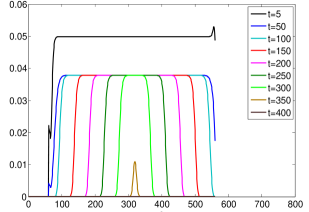
Figure 1: Profile $\phi_{a}(t)$ versus $a$ for several iteration numbers.

In order to check the prediction of state evolution, we compare the empirical and the predicted mean square errors

$${\sf MSE}_{\rm AMP} = \frac{1}{n}\|\widehat{x}^{t}(y)-\widehat{x}\|_{2}^{2},$$ (17)

$${\sf MSE}_{\rm SE} = \frac{1}{n}\sum_{i=1}^{n}{\sf mmse}\Big{(}\sum_{a\in{\sf R}}W_{a,i}\phi_{a}^{-1}(t-1)\Big{)}.$$ (18)

The values of ${\sf MSE}_{\rm AMP}$ and ${\sf MSE}_{\rm SE}$ versus iteration are depicted in Fig. 2. (Values of ${\sf MSE}_{\rm AMP}$ and the bar errors correspond to $M=30$ Monte Carlo instances). This verifies that the state evolution provides an iteration-by iteration prediction of AMP performance. We observe that ${\sf MSE}_{\rm AMP}$ (and ${\sf MSE}_{\rm SE}$) decreases linearly versus iteration.

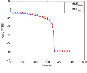
Figure 2: Comparison of ${\sf MSE}_{{\rm AMP}}$ and ${\sf MSE}_{{\rm SE}}$ across iteration.

III-B Phase diagram

In this section, we consider the noiseless compressed sensing setting, and reconstruction through different algorithms and sensing matrix ensembles.

Let $\mathcal{A}$ be a sensing matrix–reconstruction algorithm scheme. The curve ${\varepsilon}\mapsto\delta_{\mathcal{A}}({\varepsilon})$ describes the sparsity-undersampling tradeoff of ${\cal A}$ if the following happens in the large-system limit $n,m\to\infty$, with $m/n=\delta$. The scheme ${\cal A}$ does (with high probability) correctly recover the original signal provided $\delta>\delta_{\mathcal{A}}({\varepsilon})$, while for $\delta<\delta_{\mathcal{A}}({\varepsilon})$ the algorithm fails with high probability. We will consider three schemes. For each of them, we consider a set of sparsity parameters ${\varepsilon}\in\{0.1,0.2,0.3,0.4,0.5\}$, and for each value of ${\varepsilon}$, evaluate the empirical phase transition through a logit fit (we omit details, but follow the methodology described in [6]).

III-B1 Scheme I

We construct the sensing matrix as described in Section II-A and for reconstruction, we use the algorithm described in Section II-B. An illustration of the phase transition phenomenon is provided in Fig. 4. This corresponds to ${\varepsilon}=0.2$ and an estimated phase transition location $\delta=0.23$.

As it is shown in Fig. 3, our results are consistent with the hypothesis that this scheme achieves successful reconstruction at rates close to the information theoretic lower bound $\delta>\overline{d}(p_{\widehat{X}})={\varepsilon}$. (We indeed expect the gap to decrease further by taking larger values of $\ell$, $n$.)

III-B2 Scheme II

The sensing matrix $A_{{\sf F}}$ is obtained by choosing $m$ rows of the Fourier matrix ${\sf F}$ at random. In time domain, this corresponds to sampling at $m$ random time instants as in [4]. Reconstruction is done via AMP algorithm with posterior expectation as the denoiser $\eta$. More specifically, through the following iterative procedure.

$$\begin{split}\widehat{x}^{t+1}&=\eta_{t}(\widehat{x}^{t}+A^{*}r^{t})\,,\\ r^{t}&=y-A\widehat{x}^{t}+\frac{1}{\delta}r^{t-1}\langle\partial\eta_{t-1}\rangle+\frac{1}{\delta}\overline{r}^{t-1}\langle\overline{\partial}\eta_{t-1}\rangle\,.\end{split}$$ (19)

Here $\eta_{t}(v)=(\eta_{t}(v_{1}),\dots,\eta_{t}(v_{n}))$, where $\eta_{t}(v_{i})={\mathbb{E}}\{\widehat{X}|\widehat{X}+\phi_{t}^{1/2}Z=v_{i}\}$ and $Z\sim{\sf N}_{{\mathbb{C}}}(0,1)$. Also $\partial\eta_{t,i}\equiv\partial\eta_{t}(\widehat{x}_{i}^{t}+(A^{*}r^{t})_{i})$, $\overline{\partial}\eta_{t,i}\equiv\overline{\partial}\eta_{t}(\widehat{x}_{i}^{t}+(A^{*}r^{t})_{i})$ and for a vector $u\in{\mathbb{R}}^{n}$, $\langle u\rangle=n^{-1}\sum_{i=1}^{n}u_{i}$.

The sequence $\phi_{t}$ is determined by state evolution

$$\phi_{t+1}=\frac{1}{\delta}{\sf mmse}(\phi_{t}^{-1})\,,\;\;\phi_{0}={\rm Var}(\widehat{X})/\delta.$$ (20)

When $A$ has independent entries $A_{ij}\sim{\sf N}(0,1/m)$, state evolution (20) predicts the performance of the algorithm (19) [2]. Therefore, the algorithm successfully recovers the original signal with high probability, provided

$$\delta>\tilde{\delta}({\varepsilon})=\sup_{s\geq 0}s\cdot{\sf mmse}(s)\,.$$ (21)

As shown in Fig. 3, the empirical phase transition for scheme II is very close to the prediction $\tilde{\delta}({\varepsilon})$. Note that schemes I, II both use posterior expectation denoising. However, as observed in [8], spatially-coupled matrices in scheme I significantly improve the performances.

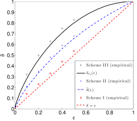
Figure 3: Phase transition lines for Schemes I, II, III.

III-B3 Scheme III

We use the spatially-coupled sensing matrix described in Section II-A, and an AMP algorithm with soft-thresholding denoiser

$$\eta_{ST}(z;\theta)=\Big{(}1-\frac{\theta}{|z|}\Big{)}_{+}z\,.$$ (22)

The algorithm is defined as in Eq. (9), except that the soft-thresholding denoiser is used in lieu of the posterior expectation. Formally, let $\eta_{t}(v)=(\eta_{t,1}(v_{1}),\cdots,\eta_{t,n}(v_{n}))$ with

$$\eta_{t,i}(v_{i})=\eta_{ST}(v_{i},\alpha^{*}({\varepsilon})s_{i}^{-1/2}),\,\;s_{i}=\sum_{a\in[m]}W_{ai}\phi_{a}(t)^{-1},$$ (23)

and the sequence of profiles $\{\phi(t)\}_{t\geq 0}$ is given by the following recursion.

$$\phi_{a}(t+1)=\sum_{i\in[n]}W_{ai}\,{\mathbb{E}}\{|\eta_{t,i}(\widehat{X}+s_{i}^{-1/2}Z;\alpha^{*}s_{i}^{-1/2})-\widehat{X}|^{2}\}.$$

Finally $\alpha^{*}=\alpha^{*}({\varepsilon})$ is tuned to optimize the phase transition boundary. This is in fact a generalization of the complex AMP (CAMP) algorithm that was developed in [12] for unstructured matrices. CAMP strives to solve the standard convex relaxation

$$\mbox{minimize}\|\widehat{x}\|_{1}=\sum_{\omega\in\Omega_{n}}|\widehat{x}(\omega)|\,,\mbox{ subject to }A_{{\sf F}}\widehat{x}=y.$$

For a given ${\varepsilon}$, we denote by $\delta_{\ell_{1}}({\varepsilon})$ the phase transition location for $\ell_{1}$ minimization, when sensing matrices with i.i.d. entries are used. This coincides with the one of CAMP with optimally tuned $\alpha=\alpha^{*}({\varepsilon})$ [18, 12].

The empirical phase transition of Scheme III is shown in Fig. 3. The results are consistent with the hypothesis that the phase boundary coincides with $\delta_{\ell_{1}}$. In other words, spatially-coupled sensing matrix does not improve the performances under $\ell_{1}$ reconstruction (or under AMP with soft-thresholding denoiser). This agrees with earlier findings by Krzakala et al. for Gaussian matrices ([8], and private communications). This can be inferred from the the state evolution map. For AMP with posterior expectation denoiser, and for ${\varepsilon}<\delta<\tilde{\delta}({\varepsilon})$, the state evolution map has two stable fixed points; one of order $\sigma^{2}$, and one much larger. Spatial coupling makes the algorithm converge to the ‘right’ fixed point. However, the state evolution map corresponding to the soft-thresholding denoiser is concave and has only one stable fixed point, much larger than $\sigma^{2}$. Therefore, spatial coupling is not helpful in this setting.

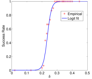
Figure 4: Phase transition diagram for Scheme I, and ${\varepsilon}=0.2$.

References

- [1] M. Bayati, M. Lelarge, and A. Montanari. Universality in message passing algorithms. submitted, 2012.
- [2] M. Bayati and A. Montanari. The dynamics of message passing on dense graphs, with applications to compressed sensing. IEEE Trans. on Inform. Theory, 57:764–785, 2011.
- [3] Y. Bresler. Spectrum-blind sampling and compressive sensing for continuous-index signals. In ITA, pages 547–554, 2008.
- [4] E. Candes, J. K. Romberg, and T. Tao. Robust uncertainty principles: Exact signal reconstruction from highly incomplete frequency information. IEEE Trans. on Inform. Theory, 52:489 – 509, 2006.
- [5] D. L. Donoho, A. Javanmard, and A. Montanari. Information-theoretically optimal compressed sensing via spatial coupling and approximate message passing. arXiv:1112.0708, 2011.
- [6] D. L. Donoho, A. Maleki, and A. Montanari. Message Passing Algorithms for Compressed Sensing. PNAS, 106:18914–18919, 2009.
- [7] A. Felstrom and K. Zigangirov. Time-varying periodic convolutional codes with low-density parity-check matrix. IEEE Trans. on Inform. Theory, 45:2181–2190, 1999.
- [8] F. Krzakala, M. Mézard, F. Sausset, Y. Sun, and L. Zdeborova. Statistical physics-based reconstruction in compressed sensing. arXiv:1109.4424, 2011.
- [9] S. Kudekar and H. Pfister. The effect of spatial coupling on compressive sensing. In 48th Annual Allerton Conference, pages 347 –353, 2010.
- [10] S. Kudekar, T. Richardson, and R. Urbanke. Threshold Saturation via Spatial Coupling: Why Convolutional LDPC Ensembles Perform So Well over the BEC. IEEE Trans. on Inform. Theory, 57:803–834, 2011.
- [11] S. Kudekar, T. Richardson, and R. Urbanke. Spatially Coupled Ensembles Universally Achieve Capacity under Belief Propagation. arXiv:1201.2999, 2012.
- [12] A. Maleki, L. Anitori, A. Yang, and R. Baraniuk. Asymptotic Analysis of Complex LASSO via Complex Approximate Message Passing (CAMP). arXiv:1108.0477, 2011.
- [13] E. Matusiak and Y. C. Eldar. Sub-Nyquist sampling of short pulses. In ICASSP, pages 3944–3947, 2011.
- [14] T. Richardson and R. Urbanke. Modern Coding Theory. Cambridge University Press, Cambridge, 2008.
- [15] P. J. Schreier and L. L. Scharf. Statistical signal processing of complex-valued data : the theory of improper and noncircular signals. Cambridge University Press, Cambridge, 2010.
- [16] A. Sridharan, M. Lentmaier, D. J. C. Jr, and K. S. Zigangirov. Convergence analysis of a class of LDPC convolutional codes for the erasure channel. In 43rd Annual Allerton Conference, Monticello, IL, Sept. 2004.
- [17] Y. Wu and S. Verdú. Rényi Information Dimension: Fundamental Limits of Almost Lossless Analog Compression. IEEE Trans. on Inform. Theory, 56:3721–3748, 2010.
- [18] Z. Yang, C. Zhang, and L. Xie. On phase transition of compressed sensing in the complex domain. IEEE Signal Processing Letters, 19:47–50, 2012.