On the Turaev-Viro Endomorphism, and the colored Jones polynomial

Abstract.

By applying a variant of the TQFT constructed by Blanchet, Habegger, Masbaum, and Vogel, and using a construction of Ohtsuki, we define a module endomorphism for each knot $K$ by using a tangle obtained from a surgery presentation of $K$. We show that it is strong shift equivalent to the Turaev-Viro endomorphism associated to $K$. Following Viro, we consider the endomorphisms that one obtains after coloring the meridian and longitude of the knot. We show that the traces of these endomorphisms encode the same information as the colored Jones polynomials of $K$ at a root of unity. Most of the discussion is carried out in the more general setting of infinite cyclic covers of 3-manifolds.

1. Introduction

1.1. History

Walker first noticed [Wa1] that the endomorphism induced in a $2+1$-TQFT (defined over a field) by the exterior of a closed off Seifert surface of a knot in zero-framed surgery along the knot can be used to give lower bounds for the genus of the knot. He did this by showing the number of non-zero eigenvalues of this endomorphism counted with multiplicity is an invariant [Wa1], i.e. it does not depend on the choice of the Seifert surface. Thus the number of such eigenvalues must be less than or equal to the dimension of the vector space that the TQFT assigns to a closed surface of this minimal genus.

Next Turaev and Viro [TV], again assuming the TQFT is defined over a field, saw that the similarity class of the induced map on the vector space associated to a Seifert surface modulo the generalized $0$-eigenspace was a stronger invariant. If the TQFT is defined over a more general commutative ring, the second author observed that the strong shift equivalence class of the endomorphism is an invariant of the knot [G3]. Strong shift equivalence (abbreviated SSE) is a notion from symbolic dynamics which we will discuss in §2.4 below. For a TQFT defined over a field $F$, the similarity class considered by Turaev-Viro is a complete invariant of SSE. In this case, the vector space modulo the generalized $0$-eigenspace together with the induced automorphism, considered as a module over $F[t,t^{-1}]$, is called the Turaev-Viro module. It should be considered as somewhat analogous to the Alexander module. The order of the Turaev-Viro module is called the Turaev-Viro polynomial and lies in $F[t,t^{-1}]$. We will refer to the endomorphisms constructed as above (and those in the same SSE class) as Turaev-Viro endomorphisms.

In [G1, G2], Turaev-Viro endomorphisms were studied and methods for computing the endomorphism explicitly were given. These methods adapted Rolfsen’s surgery technique of studying infinite cyclic covers of knots. This method requires finding a surgery description of the knot; that is a framed link in the complement of the unknot such that the framed link describes $S^{3}$ and the unknot represents the original knot. Moreover each of the components of the framed link should have linking number zero with the unknot. For this method to work, it is important that the surgery presentation have a nice form. In this paper, we will show that all knots have a surgery presentations of this form (in fact an even nicer form that we will call standard.) Another explicit method of computation was given by Achir, and Blanchet [AB]. This method starts with any Seifert surface. The second author also considered the further invariant obtained by decorating a knot with a colored meridian (this was needed to give formulas for the Turaev-Viro endomorphism of a connected sum, and to use the Turaev-Viro endomorphism to compute the quantum invariants of branched cyclic covers of the knot).

Ohtsuki [O1, O2] arrived at the same invariant as the Turaev-Viro polynomial but from a very different point of view. Ohtsuki extracts this invariant from a surgery description of a knot (alternatively of a closed 3-manifold with a primitive one dimensional cohomology class) and the data of a modular category. His method starts from any surgery description standard or not. This is a significant advantage of his approach. Ohtsuki’s proof of the invariance of the polynomial in [O1] is only sketched. He stated that his invariant is the same as the Turaev-Viro polynomial, but does not give an explanation.

Recently Viro has returned to these ideas [V1, V2]. He has studied the Turaev-Viro endomorphism of a knot after coloring both the meridian and the longitude of the knot. Viro observed that a weighted sum of the traces of these endomorphisms is the colored Jones polynomial evaluated at a root of unity.

In [G1, G2, G3], Turaev-Viro endomorphisms were defined more generally for infinite cyclic cover of 3-manifolds. Suppose $(M,\chi)$ is a closed connected oriented $3$-manifold $M$ with $\chi\in H^{1}(M,{\mathbb{Z}})$ such that $\chi:H_{1}(M,{\mathbb{Z}})\rightarrow{\mathbb{Z}}$ is onto. Let $M_{\infty}$ be the infinite cyclic cover of $M$ corresponding to $\chi$. Choose a surface $\Sigma$ in $M$ dual to $\chi$. By lifting $\Sigma$ to $M_{\infty}$, we obtain a fundamental domain $E$ with respect to the action of ${\mathbb{Z}}$ on $M_{\infty}$. $E$ is a cobordism from a surface $\Sigma$ to itself. Let $(V,Z)$ be a $2+1$-TQFT on the cobordism category of extended $3$-manifolds and extended surfaces. Applying $(V,Z)$ to $E$ and $\Sigma$, we can construct an endomorphism $Z(E):V(\Sigma)\rightarrow V(\Sigma)$. In [G3], it is proved that the strong shift equivalent class of $Z(E):V(\Sigma)\rightarrow V(\Sigma)$ is an invariant of the pair $(M,\chi)$, i.e. it does not depend on the choice of $\Sigma$. We denote this SSE class by $\mathcal{Z}(M,\chi)$. We will sometimes refer to a pair $(M,\chi)$ as above, informally, as a 3-manifold with an infinite cyclic covering.

The knot invariants discussed above can be obtained as special cases of the above invariants of 3-manifolds with an infinite cyclic covering. For any oriented knot $K$ in $S^{3}$, we obtain an extended $3$-manifold $S^{3}(K)$ by doing $0$-surgery along $K$. We choose $\chi$ to be the integral cohomology class that evaluates to $1$ on a positive meridian of $K$. Then it is easy to see that the invariant $\mathcal{Z}(S^{3}(K),\chi)$ corresponding to $(S^{3}(K),\chi)$ only depends on $K$. If our TQFT is defined for 3-manifolds with colored links, one may obtain further invariants by coloring the meridian and the longitude (a little further away) of the knot.

For the knot invariants discussed above, it is required, in general, that $K$ be oriented This is so that the exterior of a Seifert surface acquires a direction as a cobordism from the Seifert surface to itself. However, we decided to delay mentioning this technicality. To avoid issues that arise from phase anomalies in TQFT, in this paper, we work with extended manifolds as in Walker [Wa2] and Turaev [T]. In this introduction, we omit mention of the integer weights and lagrangian subspaces of extended manifolds. We discuss extended manifolds carefully in the main text.

1.2. Results of this paper

Inspired by Ohtsuki, we construct a SSE class ${Z}(M,\chi)$ from a framed ( or banded) tangle in $S^{2}\times I$ that arises in a surgery presentation of $(M,\chi)$. We call this the tangle endomorphism. Moreover we show that the endomorphism (or square matrix) that Ohtsuki considers in this situation is well defined up to SSE. By relating the definition of the Turaev-Viro endomorphism to Ohtsuki’s matrix, we give a different proof of the invariance of Ohtsuki’s invariant. In fact, we show that Ohtsuki’s matrix has the same SSE class as the Turaev-Viro endomorphism, i.e. $\mathcal{Z}(M,\chi)={Z}(M,\chi)$. We do not prove these results in the general case of a TQFT arising from a modular category. We only work in the context of the skein approach for TQFTs associated to $SO(3)$ and $SU(2)$. We work with a modified Blanchet-Habegger-Masbaum-Vogel approach [BHMV2] as outlined in [GM2]. This theory is defined over a slightly localized cyclotomic ring of integers. It is worthwhile studying endomorphisms defined up to strong shift equivalence over this ring rather than passing to a field.

We show that the traces of the Turaev-Viro polynomial of knots with the meridian and longitude colored turns out to encode exactly the same information as the colored Jones polynomial evaluated at a root of unity.

1.3. Organization of this paper

In section 2, we discuss extended manifolds, a variant of the TQFT constructed in [BHMV2], surgery presentations and the definition of SSE. In section 3, we construct an endomorphism for each framed tangle in $S^{2}\times I$ and apply it to the tangle obtained from a surgery presentation of an infinite cyclic cover of a 3-manifold. We call it the tangle endomorphism. Then we state Theorem 3.7 which states that the SSE class of a tangle endomorphism constructed from a surgery presentation of $(M,\chi)$ is an of invariant $(M,\chi)$. In section 4, we discuss technical details concerning the Turaev-Viro endomorphism for $(M,\chi)$, and the method of calculating $\mathcal{Z}(M,\chi)$ introduced in [G1]. In section 5, we relate the tangle endomorphism associated to a nice surgery presentation to the corresponding Turaev-Viro endomorphism. In section 6, we prove Theorem 3.7. In section 7, we give formulas relating the colored Jones polynomial to the traces of Turaev-Viro endomorphism of a knot whose meridian and longitude are colored. In section 8, we compute two examples to illustrate these ideas.

1.4. Convention

All surfaces and 3-mainifolds are assumed to be oriented.

2. Preliminaries

2.1. Extended surfaces and extended $3$-manifolds.

For each integer $p\geq 3$, Blanchet, Habegger, Masbaum and Vogel define a TQFT from quantum invariants of $3$-manifolds at $2p$th root of unity over a $2+1$-cobordism category in [BHMV2]. The cobordism category has surfaces with $p_{1}$-structures as objects and $3$-manifolds with $p_{1}$-structures as morphisms. They introduce $p_{1}$-structures in order to resolve the framing anomaly. Following [G4, GM2], we will adapt the theory by using extended surfaces and extended $3$-manifolds in [Wa2, T] instead of $p_{1}$-structures to resolve the framing anomaly. In the following, all homology groups have rational coefficients except otherwise stated.

Definition 2.1.

An extended surface $(\Sigma,\lambda(\Sigma))$ is a closed surface $\Sigma$ with a lagrangian subspace $\lambda(\Sigma)$ of $H_{1}(\Sigma)$ with respect to its intersection form, which is a symplectic form on $H_{1}(\Sigma)$.

Definition 2.2.

An extended $3$-manifold $(M,r,\lambda(\partial M))$ is a $3$-manifold with an integer $r$, called its weight, and whose oriented boundary $\partial M$ is given an extended surface structure with lagrangian subspace $\lambda(\partial M)$. If $M$ is a closed extended 3-manifold, we may denote the extended 3-manifold simply by $(M,r)$.

Remark 2.3.

Suppose we have an extended $3$-manifold $(M,r,\lambda(\partial M))$ and $\Sigma\subset\partial M$ is a closed surface. Then

$$\lambda(\partial M)\cap H_{1}(\Sigma)$$

need not be a lagrangian subspace of $H_{1}(\Sigma)$.

Definition 2.4.

Suppose we have an extended $3$-manifold $(M,r,\lambda(\partial M))$ and $\Sigma\subset\partial M$ is a closed surface. If $\lambda(\partial M)\cap H_{1}(\Sigma)$ is a lagrangian subspace of $H_{1}(\Sigma)$, we call $\Sigma$ equipped with this lagrangrian a boundary surface of the extended 3-manifold $(M,r,\lambda(\partial M))$.

Notation 2.5.

If $\Sigma$ is a surface, we use $\bar{\Sigma}$ to denote the surface $\Sigma$ with the opposite orientation.

Proposition 2.6.

Suppose $(V_{1},\omega_{1})$ and $(V_{2},\omega_{2})$ are two symplectic vector spaces. Consider the symplectic vector space $V_{1}\oplus V_{2}$ with symplectic form $\omega_{1}\oplus\omega_{2}$. We can identify $V_{1}$ and $V_{2}$ as symplectic subspaces of $V_{1}\oplus V_{2}$. If $\lambda\subset V_{1}\oplus V_{2}$ is a lagrangian subspace such that $\lambda\cap V_{1}$ is a lagrangian subspace of $V_{1}$, then $\lambda\cap V_{2}$ is a lagrangian subspace of $V_{2}$.

Proof.

Since $\lambda\cap V_{1}=\text{span}<a_{1},\cdots,a_{n}>$ where $n=\frac{1}{2}\text{dim}(V_{1})$, we can assume that

$$\lambda=\text{span}<(a_{1},0),\cdots,(a_{n},0),(c_{1},b_{1}),\cdots,(c_{m},b_{m})>,$$

where $m=\frac{1}{2}\text{dim}V_{2}$. Since for any $i,j$

$$0 = \omega_{1}\oplus\omega_{2}((a_{i},0),(c_{j},b_{j}))$$

$$= \omega_{1}(a_{i},c_{j})+\omega(0,b_{j})$$

$$= \omega_{1}(a_{i},c_{j}),$$

we have $c_{j}\in(\lambda\cap V_{1})^{\perp}=\lambda\cap V_{1}$. Therefore,

$$\lambda=\text{span}<(a_{1},0),\cdots,(a_{n},0),(0,b_{1}),\cdots,(0,b_{m})>.$$

That means $\text{dim}(\lambda\cap V_{2})=m$. So $\lambda\cap V_{2}$ is a lagrangian subspace in $V_{2}$. ∎

Corollary 2.7 ([GM2]).

Suppose we have an extended $3$-manifold $(M,r,\lambda(\partial M))$ and $\Sigma\subset\partial M$ is a boundary surface. Then $\partial M-\Sigma$, equipped with the lagrangian $H_{1}(\partial M-\Sigma)\cap\lambda(\partial(M))$, is also a boundary surface.

Proof.

This follows from Proposition 2.6. ∎

In the next three definitions, we describe the morphisms and the composition of morphisms in $\mathcal{C}$, a cobordism category whose objects are extended surfaces.

Definition 2.8.

Let $(M,r,\lambda(\partial M))$ be an extended $3$-manifold. Suppose

$$\partial M=\bar{\Sigma}\cup\Sigma^{\prime},$$

and this boundary has been partitioned into two boundary surfaces $\bar{\Sigma}$, called (minus) the source, and $\Sigma^{\prime}$, called the target. We write

$$(M,r,\lambda(\partial M)):(\Sigma,\lambda(\bar{\Sigma}))\rightarrow(\Sigma^{\prime},\lambda(\Sigma^{\prime})),$$

and call $(M,r,\lambda(\partial M))$ an extended cobordism.

Definition 2.9.

Let $\Sigma$ be a boundary surface of an extended $3$-manifold $(M,r,\lambda(\partial M))$ with inclusion map

$$i_{\Sigma,M}:\Sigma\rightarrow M.$$

Let $\Sigma^{\prime}$ be $\partial M-\Sigma$ with inclusion map

$$i_{\Sigma^{\prime},M}:\Sigma^{\prime}\rightarrow M.$$

Then we define

$$\lambda_{M}(\Sigma)=i^{-1}_{\Sigma,M}(i_{\Sigma^{\prime},M}(\lambda(\Sigma^{\prime}))).$$

We define the composition of morphisms in $\mathcal{C}$ as the extended gluing of cobordisms.

Definition 2.10.

Let $(M,r,\lambda(\partial M))$ and $(M^{\prime},r^{\prime},\lambda(\partial M^{\prime}))$ be two extended $3$-manifolds. Suppose $(\Sigma,\lambda(\Sigma))$ is a boundary surface of $(M,r,\lambda(\partial M))$ and $(\bar{\Sigma},\lambda(\Sigma))$ is a boundary surface of $(M^{\prime},r^{\prime},\lambda(\partial M^{\prime}))$. Then we can glue $(M,r,\lambda(\partial M))$ and $(M^{\prime},r^{\prime},\lambda(\partial M^{\prime}))$ together with the orientation reversing identity from $\Sigma$ to $\bar{\Sigma}$ to form a new extended $3$-manifold. The new extended $3$-manifold has

1. base manifold: $M\cup_{\Sigma}M^{\prime}$

2. lagrangian subspace:

   $$[\lambda(\partial M)\cap H_{1}(\partial M-\Sigma)]\oplus[\lambda(\partial M^{\prime})\cap H_{1}(\partial M^{\prime}-\bar{\Sigma})],$$

3. weight:

   $$r+r^{\prime}-\mu(\lambda_{M}(\Sigma),\lambda(\Sigma),\lambda_{M^{\prime}}(\bar{\Sigma})),$$

   where $\mu$ is the Maslov index as in [T].

Definition 2.11.

Let $(M,r,\lambda(\partial M))$ be an extended $3$-manifold with a boundary surface of the form $\Sigma\cup\bar{\Sigma}$. Then we define the extended $3$-manifold obtained by gluing $\Sigma$ and $\bar{\Sigma}$ together to be the extended $3$-manifold that results from gluing $(M,r,\lambda(\partial M))$ and $(\Sigma\times[0,1],0,\lambda(\Sigma\cup\bar{\Sigma}))$ along $\Sigma\cup\bar{\Sigma}$. In the special case that $\partial M=\Sigma\cup\bar{\Sigma}$, we call the resulting extended $3$-manifold the closure of $(M,r,\lambda(\partial M))$.

Remark 2.12.

One should think of the weight of an extended $3$-manifold $M$ as the signature of some background $4$-manifold [Wa2]. See also [G4, p. 399].

Lemma 2.13.

Let $(R,r,\lambda(\partial R))$ be a morphism from $(\Sigma,\lambda(\Sigma))$ to $(\Sigma^{\prime},\lambda(\Sigma^{\prime}))$ and $(S,s,\lambda(\partial S))$ be a morphism from $(\Sigma^{\prime},\lambda(\Sigma^{\prime}))$ to $(\Sigma,\lambda(\Sigma))$. Then the extended $3$-manifold we obtain by gluing $(R,r,\lambda(\partial R))$ to $(S,s,\lambda(\partial S))$ along $\Sigma^{\prime}$ first and then closing it up along $\Sigma$ is the same as the one we obtained from gluing $(S,s,\lambda(\partial S))$ to $(R,r,\lambda(\partial R))$ along $\Sigma$ first and then closing it up along $\Sigma^{\prime}$.

Proof.

This can be seen from $4$-manifold interpretation of weights in [Wa2, GM2].∎

Extended surfaces may also be equipped with banded points: this is an embedding of the disjoint union of oriented intervals. By a framed link, we will mean what is called a banded link in [BHMV2, p.884], i.e. an embedding of the disjoint union of oriented annuli. Framed $1$-manifold are defined similarly. Extended $3$-manifolds are sometimes equipped with framed links, or framed 1-manifolds or more generally trivalent fat graphs. By a trivalent fat graphs, we will mean what is called a banded graph in [BHMV2, p.906]. The framed links, framed 1-manifolds and trivalent fat graphs must meet the boundary surfaces of a 3-manifold in banded points with the induced “banding”. Of course, we could have used the word “banded” in all cases, but the other terminology is more common.

There is a surgery theory for extended $3$-manifolds. We refer the reader to [GM2, §2]. Here we give extended version of Kirby moves [K]. These moves relate framed links in $S^{3}$ where $S^{3}$ is itself equipped with an integer weight. The result of extended surgery of $S^{3}$ with its given weight along the link is preserved by these moves. Moreover (but we do not use this) if surgery along two framed links in weighted copies of $S^{3}$ result in the same extended manifold then there is sequence of extended Kirby moves relating them.

Definition 2.14.

The extended Kirby-$1$ move is the regular Kirby-$1$ move with weight of manifold changed accordingly. More specifically, if we add an $\epsilon$-framed unknot to the surgery link, then we change the weight of the manifold by $-\epsilon$, where $\epsilon=\pm 1$. If we delete an $\epsilon$-framed unknot from the surgery link, then we change the weight of the manifold by $\epsilon$. The extended Kirby-$2$ move is the regular Kirby-$2$ move with the weight remaining the same.

2.2. A variant of the TQFT of Blanchet, Habegger, Masbaum and Vogel.

Suppose a closed connected $3$-manifold $M$ is obtained from $S^{3}$ by doing surgery along a framed link $L$, then $(M,r)$ is obtained from $(S^{3},r-\sigma(L))$ by doing extended surgery along $L$. Here $\sigma(L)$ is the signature of the linking matrix of $L$. Warning this is different than the signature of $L$ . The quantum invariant of $(M,r)$ at a $2p$th root of unity $A$ is then defined as:

$$Z((M,r))=\eta\kappa^{r-\sigma(L)}<L(\omega)>,$$

where

$$\Delta_{k}=<U(e_{k})>,\hskip 7.22743pt\eta^{-1}=\sqrt{\sum_{k}\Delta_{k}^{2}},\hskip 7.22743pt\omega=\sum_{k}\eta\Delta_{k}e_{k},\hskip 7.22743pt\kappa=<U_{+}(\omega)>.$$

We use $<\ >$ to denote the Kauffman bracket evaluation of a linear combination of colored links in $S^{3}$, and $\mathcal{L}(x)$ to denote the satellization of a framed link $\mathcal{L}$ by a skein $x$ of the solid torus. Moreover $e_{k}$ denotes the skein class in the solid torus obtained by taking the closure of $f_{k}$, the Jones-Wenzl idempotent in the $k$-strand Temperley-Lieb algebra. Here $U$ denotes the zero framed unknot and $U_{+}$ is the unknot with framing $+1$. The sum is over the colors $0\leq k\leq p/2-2$ if $p$ is even and $0\leq k\leq p-3$ with $k$ even if $p$ is odd. One has that $\kappa$ is a square root of $A^{-6-p(p+1)/2}$. The choice of square root here determines the choice in the square root in the formula of $\eta^{-1}$, or vice-versa. See the formula for $\eta$ in [BHMV2, page 897]. The closed connected manifold $M$ may also have an embedded $p$-admissibly colored fat trivalent graph $G$ in the complement of the surgery, then

$$Z((M,r),G)=\eta\kappa^{r-\sigma(L)}<L(\omega)\cup G>.$$

By following the exactly the same procedure in [BHMV2], we can construct a TQFT for the category of extended surfaces and extended $3$-manifolds from quantum invariants. The TQFT assigns to each extended surface $(\Sigma,\lambda(\Sigma))$, possibly with some banded colored points, a module $V(\Sigma,\lambda(\Sigma))$ over $k_{p}={\mathbb{Z}}[{\frac{1}{p}},A,\kappa]$, and assigns to each extended cobordism $M$, with a $p$-admissibly colored trivalent fat graph meeting the banded colored points,

$$(M,r,\lambda(M)):(\Sigma,\lambda({\Sigma}))\rightarrow(\Sigma^{\prime},\lambda(\Sigma^{\prime}))$$

a $k_{p}$-module homomorphism:

$$Z((M,r,\lambda(M))):V((\Sigma,\lambda({\Sigma}))\rightarrow V((\Sigma^{\prime},\lambda(\Sigma^{\prime}))).$$

Then by using this TQFT, we can produce a Turaev-Viro endomorphism associated to each weighted closed 3-manifold equipped with a choice of infinite cyclic cover using the procedure described in §1.

Notation 2.15.

We introduce some notations that will be used later.

1. $\Lambda^{(l)}_{k}=\eta^{l}\Delta^{l}_{k}f_{k}$,

2. $\omega^{(l)}=\sum_{k}\eta^{l}\Delta^{l}_{k}e_{k}$,

3. $\Theta(a,b,c)$ is the Kauffman bracket of the left diagram in Figure 1,

4. $Tet(a,b,c,d,e,f)$ is the Kauffman bracket of the right diagram in Figure 1.

Figure 1. On the left is $\Theta(a,b,c)$, and on the right is ${\operatorname{Tet}}(a,b,c,d,e,f)$.

2.3. Surgery presentations

The earliest use of surgery presentations, that we are aware of, was by Rolfsen [R1] to compute and study the Alexander polynomial. In this paper we consider surgery descriptions for extended closed 3-manifolds with an infinite cyclic cover. We will use these descriptions for extended 3-manifolds that contain certain colored trivalent fat graphs. As this involves no added difficulty, we will not always mention these graphs in this discussion.

Definition 2.16.

Let $K_{0}\cup L$ be a framed link inside $(S^{3},s)$ where $K_{0}$ is an oriented $0$-framed unknot, and the linking numbers of the components of $L$ with $K_{0}$ are all zero. Let $D_{0}$ be a disk in $S^{3}$ with boundary $K_{0}$ which is transverse to $L$. Suppose $(M,r)$ is the result of extended surgery along $K_{0}\cup L$, then there exists a unique epimorphism $\chi:H_{1}(M,{\mathbb{Z}})\rightarrow{\mathbb{Z}}$ which agrees with the linking number with $K_{0}$ on cycles in $S^{3}\setminus(K_{0}\cup L)$. We will call $(D_{0},L,s)$ a surgery presentation of $((M,r),\chi)$. We remark that, in this situation, we will have $s=r-\sigma(L)$. If there are graphs $G^{\prime}$ in $M$ and $G$ in $S^{3}\setminus(K_{0}\cup L)$ (transverse to $D_{0}$) related by the surgery, we will say $(D_{0},L,s,G)$ a surgery presentation of $((M,r),\chi,G^{\prime})$.

If the result of surgery along $L$ returns $S^{3}$ with the image of $K_{0}$ after surgery becoming a knot oriented knot $K$, and the linking numbers of the components of $L$ with $K_{0}$, then $K_{0}\cup L$ is a surgery presentation of $K$ as in Rolfsen. The manifold obtained by surgery along $K_{0}\cup L$ in $S^{3}$ is the same as $0$-framed surgery along $K$ in $S^{3}$.

The following Proposition is proved in section 4 of [O1] for non-extended manifolds. The extended version involves no extra difficulty

Proposition 2.17.

Every extended connected $3$-manifold with an epimorphism $\chi:H_{1}(M,{\mathbb{Z}})\rightarrow{\mathbb{Z}}$ has a surgery presentation.

Every surgery presentation can be described by diagram as in Figure 2 which we will refer to as a surgery presentation diagram.

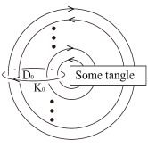
Figure 2. A surgery presentation diagram. Of course, the tangle must be such that each closed component of $L$ has zero linking number with $K_{0}$. Notice the orientation on $K_{0}$.

Definition 2.18.

If a surgery presentation diagram is in the form of Figure 3, then we say this surgery presentation diagram is in standard form. We will also say that a surgery presentation $(D_{0},L,s,G)$ is standard if it has a surgery presentation diagram in standard form.

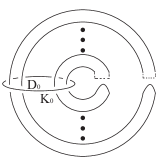
Figure 3. The dotted part could be knotted or linked with other strands within the tangle box. The bottom turn-backs are simple arcs without double points under the projection. Each component of $L$ intersects the flat disc $D_{0}$ bounded by the trivial knot algebraically $0$ times, but geometrically $2$ times.

Ohtsuki [O1, bottom of p. 259] stated a proposition about surgery presentations of knots which is similar to the following proposition. Our proof is similar to the proof that Ohtsuki indicated. We will call a Kirby-$1$ move in a surgery presentation a small Kirby-$1$ move if a disk which bounds the created or deleted component is in the complement of $D_{0}$. We will call a Kirby-$2$ move in a surgery presentation a small Kirby-$2$ move if it involves sliding a component other than $K_{0}$ over another component that is in the complement of $D_{0}$. A $D_{0}$-move is a choice of a new spanning disk $D^{\prime}$ with $D_{0}\cap D^{\prime}=K_{0}$ followed by an ambient isotopy that moves $D^{\prime}$ to the original position of $D_{0}$ and moves $L$ at the same time.

Proposition 2.19.

A surgery presentation described by a surgery presentation diagram can be transformed into a surgery presentation described by a surgery presentation diagram in standard form by a sequence of isotopies of $L\cup G$ relative to $D_{0}$, small Kirby-$1$ moves, small Kirby-$2$ moves, and $D_{0}$-moves. Therefore, every extended $3$-manifold with an epimorphism $\chi:H_{1}(M,{\mathbb{Z}})\rightarrow{\mathbb{Z}}$ has a standard surgery presentation.

Proof.

We need to prove that we can change a surgery presentation described by a surgery diagram as in Figure 2 into surgery presentation described by a diagram as in Figure 3 using the permitted moves.

Let

$$m=\max_{L_{i}\text{\ is a component of\ }L}|L_{i}\cap D_{0}|.$$

We will prove the theorem by induction on $m$. Since each component $L_{i}$ has linking number 0 with $K_{0}$, it is easy to see that $m$ is even.

If $m=0$, then $L$ can be taken to be contained in the tangle box.

When $m=2$, we may

• first do a $D_{0}$ move to shift $D_{0}$ slightly;

• then perform an isotopy relative to the new $D_{0}$ of $L$ so that the points on intersection of the image of the old $D_{0}$ with each components of $L$ are adjacent to each other;

• then do another $D_{0}$-move to move the old $D_{0}$ back to its original position.

Now the arcs emitted from the bottom edge of the tangle are in a correct order. But the diagram in Figure 2 may differ from a standard tangle in the way that the arcs emitted from bottom edge of the tangle box are not in the specified simple form. This means they could be knotted and linked with each other. However we may perform small Kirby-$1$ and small Kirby-$2$ moves as in Figure 4 to unknot and unlink these arcs so that the resulting diagram has standard form.

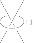
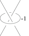
Figure 4. We use $+1$ or $-1$ surgery on unknot to change the crossing.

We now prove that the theorem holds for all links with $m=2n$ where $n\geq 2,$ assuming it holds for all links with $m\leq 2n-2$. Suppose the component $L_{1}$ intersects $D_{0}$ geometrically $2n$ times. Because $L_{1}$ has linking number $0$ with $K_{0}$, we have that at least one arc, say $\alpha$ of $L_{1}$ in Figure 2 which joins two points on the bottom of the tangle box, i.e. it is a “turn-back”. For each crossing with exactly one arc from $\alpha$, we can make the arc $\alpha$ to be the top arc (in the direction perpendicular to the plane of the diagram) by using the moves of Figure 4, which just involve some small Kirby-$1$ and small Kirby-$2$ moves. Then it is only simply linked to other components by some new trivial components with framing $\pm 1$. Then by using isotopies relative to $D_{0}$, we can slide the arc $\alpha$ towards bottom of the tangle, with the newly created unknots stretched vertically in the diagram so that they intersect each horizontal cross-section in at most 2-points. See the central illustration Figure 5 where $\alpha$ is illustrated by two vertical arcs meeting a small box labeled $X$. This small box contains the rest of $\alpha$. Now perform a $D_{0}$ move which has the effect of pulling the turn-back across $D_{0}$. Those trivial components will follow the turn back and pass through $D_{0}$. But since at the beginning, those components have geometric intersection $0$ with $D_{0}$, they have geometric intersection $2$ with $D_{0}$ now. After this process, $L_{1}\cap D_{0}$ is reduced by $2$. This process does not change the number of intersections with $D_{0}$ of the other components of the original $L$.

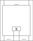
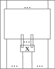
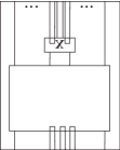
Figure 5. Moves which reduce the number of intersections of a component of $L$ with $D_{0}$. We perform small K-moves and isotopies to change to the middle picture. We perform a $D_{0}$-move to change to the right hand picture.

We do this process for all components $L_{j}$ with $|L_{j}\cap D_{0}|=2n$. Then the new link has $m\leq 2n-2$. By our induction hypothesis, we can transform $K_{0}\cup L$ into a standard form using the allowed moves. ∎

2.4. Strong shift equivalence.

We will discuss SSE in the category of free finitely generated modules over a commutative ring with identity. This notion arose in symbolic dynamics. For more information, see [Wag, LM] and references therein.

Definition 2.20.

Suppose

$$X:V\rightarrow V,Y:U\rightarrow U$$

are module endomorphisms. We say $X$ is elementarily strong shift equivalent to $Y$ if there are two module morphisms

$$R:V\rightarrow U,S:U\rightarrow V$$

such that

$$X=SR,Y=RS.$$

We denote this by $X\approx Y$.

Definition 2.21.

Suppose

$$X:V\rightarrow V,Y:U\rightarrow U$$

are module endomorphisms. We say $X$ is strong shift equivalent to $Y$ if there are finite number of module endomorphisms $\{X_{1},...,X_{n}\}$ such that

$$X\approx X_{1}\approx X_{2}...\approx X_{n}\approx Y.$$

We denote this by $X\sim Y$.

It is easy to see that if $X\sim Y$, then ${\operatorname{Trace}}(X)={\operatorname{Trace}}(Y)$.

Proposition 2.22.

Let $X$ be a module endomorphism of $V$. Suppose $V=U\oplus W$ where $U$ and $W$ are free finitely generated modules such that $U$ in the kernel of $X$, and let $\hat{X}$ be the induced endomorphism of $W$, then $\hat{X}$ is SSE to $X.$

Proof.

Suppose ${\operatorname{Rank}}(U)=m$, and ${\operatorname{Rank}}(W)=n$. The result follows from the following block matrix equations.

$$\left[\begin{array}[]{c}v_{m\times n}\\ \hline\cr\hat{X}_{n\times n}\end{array}\right]_{(n+m)\times n}\cdot\left[\begin{array}[]{c|c}0_{n\times m}&I_{n}\end{array}\right]_{n\times(n+m)}=\left[\begin{array}[]{c|c}0_{m\times m}&v_{m\times n}\\ \hline\cr 0_{n\times m}&\hat{X}_{n\times n}\end{array}\right]_{(n+m)\times(n+m)}$$

$$\left[\begin{array}[]{c|c}0_{n\times m}&I_{n}\end{array}\right]_{n\times(n+m)}\cdot\left[\begin{array}[]{c}v_{m\times n}\\ \hline\cr\hat{X}_{n\times n}\end{array}\right]_{(n+m)\times n}=\left[\hat{X}_{n\times n}\right]_{n\times n}$$

∎

If $T$ is an endomorphism of a vector space $V$, let $N(T)$ denote the generalized $0$-eigenspace for $T$, and $T_{\flat}$ denote the induced endomorphism on $V/N(T)$. The next proposition may be deduced from more general statements made in [BH, p. 122, Prop(2.4) ]. For the convenience of the reader, we give direct proof.

Proposition 2.23.

Let $T$ and $T^{\prime}$ be endomorphisms of vector spaces. $T$ and $T^{\prime}$ are SSE if and only if $T_{\flat}$ and $T_{\flat}^{\prime}$ are similar.

Proof.

The only if implication is well-known [LM, Theorem 7.4.6]. The if implication follows from the easy observations that similar transformations are strong shift equivalent and that $T$ is strong shift equivalent to $T_{\flat}$. This second fact follows from the repeated use of the following observation: If $x\neq 0$ is in the null space of $T$, $<x>$ denotes the space spanned by $x$, and $T_{x}$ denotes the induced map on $V/<x>$, then $T$ and $T_{x}$ are strong shift equivalent. This follows from Proposition 2.22 with $U=<x>$. ∎

3. The tangle morphism

In this section, we will assign a $k_{p}$-module homomorphism to any framed tangle in $S^{2}\times I$ enhanced with an embedded $p$-admissibly colored trivalent fat graph in the complement of the tangle. By slicing a surgery presentation for an infinite cyclic cover of an extended $3$-manifold and applying the TQFT, we obtain such a tangle, and thus a $k_{p}$-module endomorphism. The idea of constructing this endomorphism is inspired by the work of Ohtsuki in [O1].

There is a unique lagrangian for a 2-sphere. Thus we can consider any 2-sphere as an extended manifold without specifying a lagrangian. Similarly, we let $(S^{2}\times I,r)$ denote the extended manifold $S^{2}\times I$ with weight $r$, as there is no need to specify a lagrangian.

Definition 3.1.

Let $S$ be a 2-sphere equipped with $m$ ordered uncolored banded points, and $u$ ordered banded points colored by $x_{1},\cdots,x_{u}$. We define $S(i_{1},i_{2},\cdots i_{m})$ to be this 2-sphere where the $m$ uncolored banded points have been colored by $(i_{1},i_{2},\cdots i_{m})$ (and the $u$ points already colored remain colored).

We define

$$V(S)=\sum_{i_{1},...,i_{m}}V(S(i_{1},i_{2},\cdots i_{m})).$$

Here $V(S(i_{1},i_{2},\cdots i_{m}))$ is the module for a extended 2-sphere with $m$ uncolored banded points colored by $(i_{1},\cdots,i_{m})$ and $u$ banded points colored by $(x_{1},\cdots,x_{u})$ obtained by applying the TQFT that we introduced in §2.

By an $(m,n)$-tangle in $(S^{2}\times I,r)$, we mean a properly embedded framed 1-manifold in $(S^{2}\times I,r)$ with $m$ endpoints on $S_{0}=S^{2}\times\{0\}$, $n$ points on $S_{1}=S^{2}\times\{1\}$, with possibly some black dots on its components and a (possibly empty) colored trivalent fat graph (in the complement of the 1-manifold) meeting $S_{0}$ in $u$ colored points $x_{1},\cdots,x_{u}$ and meeting $S_{1}$ in $t$ colored points $y_{1},\cdots,y_{t}$. Thus $S_{0}$ is a 2-sphere with $m$ ordered uncolored banded points and $u$ colored banded points. Similarly $S_{1}$ is a 2-sphere with $n$ ordered uncolored banded points and $t$ colored banded points. For any $(m,n)$-tangle, we will define a homomorphism from ${V(S_{0})}$ to ${V(S_{1})}$.

Before doing that, we introduce some definitions. From now on, we will not explicitly mention the banding on the selected points of a surface or the framing of a tangle, or the fattening of a trivalent graph. Each comes equipped with such and the framing/fattening of a link/graph induces the banding on its boundary points. Nor will we mention the ordering chosen for uncolored sets of points.

Definition 3.2.

Suppose we have a $(m,n)$-tangle in $(S^{2}\times I,r)$ with a colored trivalent graph with $u$ edges colored by $x_{1},\cdots,x_{u}$ meeting $S^{2}\times\{0\}$ and $t$ edges colored by $y_{1},\cdots,y_{t}$ meeting $S^{2}\times\{1\}$. Suppose we color the $m$ endpoints from the tangle on $S_{0}=S^{2}\times\{0\}$ by $i_{1},\cdots,i_{m}$ and color the $n$ endpoints from the tangle on $S_{1}=S^{2}\times\{1\}$ by $j_{1},\cdots,j_{n}$. We say that the coloring $(i_{1},\cdots,i_{n},j_{1},\cdots,j_{m})$ is legal if the two endpoints of the same strand have the same coloring. We denote the tangle with the endpoints so-colored by $T^{n,(j_{1},...,j_{n})}_{m,(i_{1},...,i_{m})}$. For an example, see Figure 6.

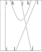
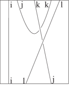
Figure 6. The coloring in first diagram is a legal coloring and the one in the second diagram is a illegal coloring for $k\neq j$. In this example, the colored trivalent graph is empty.

Definition 3.3.

Suppose we have $T^{n,(j_{1},...,j_{n})}_{m,(i_{1},...,i_{m})}$, a $(i_{1},\cdots,i_{m},j_{1},\cdots,j_{n})$ colored $(m,n)$-tangle as in Definition 3.2. We define a homomorphism

$${V(S_{0}(i_{1},\cdots,i_{m}))}\stackrel{{\scriptstyle{Z(T^{n,(j_{1},...,j_{n})}_{m,(i_{1},...,i_{m})})}}}{{\longrightarrow}}{V(S_{1}(j_{1},\cdots,j_{n}))}$$

as follows.

• If $(i_{1},\cdots,i_{m},j_{1},\cdots,j_{n})$ is a illegal coloring. We take the homomorphism to be the zero homomorphism.

• If $(i_{1},\cdots,i_{m},j_{1},\cdots,j_{n})$ is a legal coloring. We decorate uncolored components of the tangle by some skeins in $2$ cases:

  1. If there are $l$ black dots on the component, $l\in\{0,1,2,\cdots\}$, and the component has two endpoints with color $k$, $k\in\{i_{1},\cdots,i_{m},j_{1},\cdots,j_{n}\}$, then we decorate the component by $\Lambda^{(l)}_{k}$.

  2. If there are $l$ black dots on the component, $l\in\{0,1,2,\cdots\}$, and the component lies entirely in $S^{2}\times(0,1)$, then we decorate the component by $\omega^{(l)}$.

  Then we apply $Z$ to $(S^{2}\times I,r)$ with the tangle ${T^{n}_{m}}$, so decorated, to get the morphism ${Z(T^{n,(j_{1},...,j_{n})}_{m,(i_{1},...,i_{m})})}$.

Now we are ready to define the homomorphism for a tangle ${T^{n}_{m}}$.

Definition 3.4.

Suppose we have a $(m,n)$-tangle ${T^{n}_{m}}$. We define the homomorphism for the tangle, denoted by ${Z(T^{n}_{m})}$, to be

$${V(S_{0})}\stackrel{{\scriptstyle\sum{Z(T^{n,(j_{1},...,j_{n})}_{m,(i_{1},...,i_{m})})}}}{{\longrightarrow}}{V(S_{1})}$$

where ${Z(T^{n,(j_{1},...,j_{n})}_{m,(i_{1},...,i_{m})})}$ is as in Definition 3.3 and the sum runs over all colorings $(i_{1},\cdots,i_{m},j_{1},\cdots,j_{n})$.

Proposition 3.5.

For a tangle $T_{1}$ in $(S^{2}\times I,r)$ and a tangle $T_{2}$ in $(S^{2}\times I,s)$, we have

$$Z(T_{2}\circ T_{1})=Z(T_{2})Z(T_{1}),$$

where $T_{2}\circ T_{1}$ in $(S^{2}\times I,r+s)$ means gluing $T_{2}$ on the top of $T_{1}$. Here, of course, we assume that the top of $T_{1}$ and the bottom of $T_{2}$ agree.

Proof.

This follows from the functoriality of the original TQFT. ∎

Now we can construct tangle endomorphisms for an extended closed $3$-manifold with an embedded colored trivalent graph, and choice of infinite cyclic cover. Given $((M,r),\chi,G^{\prime})$, we choose a surgery presentation $(D_{0},L,s,G)$. We put one black dot somewhere on each component of $L$ away from $D_{0}$. By doing a $0$-surgery along $K_{0}$, we obtain $(S^{2}\times S^{1},s)$ with link $L$ and trivalent graph $G$, where $D_{0}$ can be completed to $S^{2}\times\{p\}$ for some point $p$ on $S^{1}$. We cut $S^{2}\times S^{1}$ along $S^{2}\times\{p\}$ . Then we obtain a tangle $\mathcal{T}^{n}_{n}$ in $(S^{2}\times I,s)$. Here $n=|\mathcal{T}^{n}_{n}\cap(S^{2}\times\{1\})|=|\mathcal{T}^{n}_{n}\cap(S^{2}\times\{0\})|$. Let $Z(\mathcal{T}^{n}_{n})$ denote tangle endomorphism associated to $\mathcal{T}^{n}_{n}$.

Lemma 3.6.

If $\mathcal{T}^{n}_{n}$ is constructed as above, then the SSE class of $Z(\mathcal{T}^{n}_{n})$ is independent of the positioning of the black dots.

Proof.

By definition, we can move a black dot on the component of the tangle $\mathcal{T}^{n}_{n}$ anywhere without changing the tangle endomorphism $Z(\mathcal{T}^{n}_{n})$. We move the black dot to near bottom or near top and cut the tangle $\mathcal{T}^{n}_{n}$ into two tangles $S$ and $T$, where $T$ is a trivial tangle with the black dot. For an example, see Figure 7. Then we switch the position of $S$ and $T$ and move the black dot in resulting tangle to near the other end of that component. Then we do the process again. By doing this, we can move it to any arc of the tangle $\mathcal{T}^{n}_{n}$, which belongs to the same component of the link $L$. But for each step, $Z(ST)=Z(S)Z(T)$ is strong shift equivalent to $Z(TS)=Z(T)Z(S)$. Therefore, the lemma is true. ∎

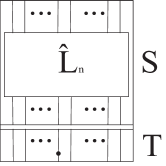
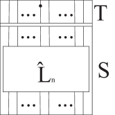
Figure 7. Here $T$ is the trivial part with the black dot.

Thus the SSE class of the tangle endomorphism $Z(\mathcal{T}^{n}_{n})$ constructed as above depends only on a surgery presentation $(D_{0},L,s,G)$. Thus we can denote this class by $Z(D_{0},L,s,G)$.

Theorem 3.7.

Let $(D_{0},L_{1},s_{1},G_{1})$ and $(D_{0},L_{2},s_{2},G_{2})$ be two surgery presentations for $((M,r),\chi,G^{\prime})$, an extended closed $3$-manifold with an embedded colored trivalent graph, and choice of infinite cyclic cover. Then

$$Z(D_{0},L_{1},s_{1},G_{1})=Z(D_{0},L_{2},s_{2},G_{2}).$$

Thus we may denote this SSE class by $Z((M,r),\chi,G^{\prime})$.

This theorem will be proved in section 6, after the way has been prepared in sections 4 and, 5.

4. The Turaev-Viro endomorphism

In §1, we introduced the basic idea of the Turaev-Viro endomorphism. In this section, we will include the technical details.

Remark 4.1.

The discussion in this section and the next section works for $3$-manifolds with an embedded $p$-admissibly colored trivalent graph. For simplicity, we usually omit mention of the trivalent graph. Thus we will write $((M,r),\chi)$ instead of $((M,r),\chi,G^{\prime})$. This is according to the philosophy that we should think of the colored trivalent graph $G^{\prime}$ as simply some extra structure on $M$.

Lemma 4.2.

Let $(M,r,\lambda(\partial M)_{1})$ be an extended cobordism from $(\Sigma,\lambda(\Sigma)_{1})$ to itself and $(M,r,\lambda(\partial M)_{2})$ be an extended cobordism from $(\Sigma,\lambda(\Sigma)_{2})$ to itself. Then $Z((M,r,\lambda(\partial M)_{1}))$ is strong shift equivalent to $Z((M,r,\lambda(\partial M)_{2}))$.

Proof.

First we notice that

$$\lambda(\partial M)_{1}=\lambda(\Sigma)_{1}\oplus\lambda(\Sigma)_{1}\in H_{1}(\Sigma)\oplus H_{1}(\bar{\Sigma}),$$

$$\lambda(\partial M)_{2}=\lambda(\Sigma)_{2}\oplus\lambda(\Sigma)_{2}\in H_{1}(\Sigma)\oplus H_{1}(\bar{\Sigma}).$$

Then we have

$$(M,r,\lambda(\partial M)_{1})$$

$$=(\Sigma\times I,0,\lambda(\Sigma)_{1}\oplus\lambda(\Sigma)_{2})\cup_{(\Sigma,\lambda(\Sigma)_{2})}(M,r,\lambda(\Sigma)_{2}\oplus\lambda(\Sigma)_{1}),$$

$$(M,r,\lambda(\partial M)_{2})$$

$$=(M,r,\lambda(\Sigma)_{2}\oplus\lambda(\Sigma)_{1})\cup_{(\Sigma,\lambda(\Sigma)_{1})}(\Sigma\times I,0,\lambda(\Sigma)_{1}\oplus\lambda(\Sigma)_{2}).$$

Here we consider $(M,r,\lambda(\Sigma)_{2}\oplus\lambda(\Sigma)_{1})$ as a cobordism from $(\Sigma,\lambda(\Sigma)_{2})$ to $(\Sigma,\lambda(\Sigma)_{1})$. Then by the functoriality of $Z$, we have the conclusion. ∎

Lemma 4.3.

Suppose we have a closed extended 3-manifold $((M,r),\chi)$ with an infinite cyclic covering. We obtain two extended fundamental domains $M_{1}$ and $M_{2}$ by slicing along two extended surfaces $(\Sigma,\lambda(\Sigma))$ and $(\Sigma^{\prime},\lambda(\Sigma^{\prime}))$ which are dual to $\chi$. We obtain two morphisms

$$(M_{1},r_{1},\lambda(\Sigma)\oplus\lambda(\Sigma)):(\Sigma,\lambda(\Sigma))\rightarrow(\Sigma,\lambda(\Sigma)),$$

$$(M_{2},r_{2},\lambda(\Sigma^{\prime})\oplus\lambda(\Sigma^{\prime})):(\Sigma^{\prime},\lambda(\Sigma^{\prime}))\rightarrow(\Sigma^{\prime},\lambda(\Sigma^{\prime})),$$

with weight $r_{1},r_{2}$ respectively such that the closures of both cobordism having weight $r$. Then

$$Z((M_{1},r_{1},\lambda(\Sigma)\oplus\lambda(\Sigma)))\sim Z((M_{2},r_{2},\lambda(\Sigma^{\prime})\oplus\lambda(\Sigma^{\prime})).$$

Proof.

We just need prove the case where $\Sigma$ and $\Sigma^{\prime}$ are disjoint from each other. See [L1, Proof of Theorem 8.2], [G3]. Since $\Sigma^{\prime}$ is disjoint from $\Sigma$, we can choose a copy of $(\Sigma^{\prime},\lambda(\Sigma^{\prime}))$ inside $(M_{1},r_{1},\lambda(\Sigma)\oplus\lambda(\Sigma))$. We cut along $\Sigma^{\prime}$ and get two $3$-manifolds $T,S$. We assign to $T,S$ extended $3$-manifold structures, denoted by $(T,t,\lambda(\Sigma)\oplus\lambda(\Sigma^{\prime}))$ and $(S,s,\lambda(\Sigma^{\prime})\oplus\lambda(\Sigma))$, such that if we glue $R$ to $S$ along $\Sigma^{\prime}$, we get $(M_{1},r_{1},\lambda(\Sigma)\oplus\lambda(\Sigma))$ back. We need to choose appropriate weights $t,s$ for $T,S$. Using Definition 2.10, we see that such $t,s$ exists. Now we just need prove that if we glue $S$ to $T$ along $\Sigma$, we obtain $(M_{2},r_{2},\lambda(\Sigma^{\prime})\oplus\lambda(\Sigma^{\prime}))$. Actually, it is easy to see that after gluing, we have the right base manifold and lagrangian subspace. What we need to prove is that we get the right weight. This follows from Lemma 2.13. ∎

As a consequence of the two lemmas above, we have the following:

Proposition 4.4.

For a tuple $((M,r),\chi)$ and $(M_{1},r_{1},\lambda(\Sigma_{1})\oplus\lambda(\Sigma_{1}))$ given as in Lemma 4.3, the strong shift equivalent class of the map $Z((M_{1},r_{1},\lambda(\Sigma_{1})\oplus\lambda(\Sigma_{1})))$ is independent of the choice of the extended surface $(\Sigma_{1},\lambda(\Sigma_{1}))$. Thus we may denote this SSE class by $\mathcal{Z}((M,r),\chi)$.

Next, we work towards constructing a fundamental domain for an extended $3$-manifold $((M,r),\chi)$ with an infinite cyclic covering. Suppose we have a surgery presentation $(D_{0},L,s)$ in standard form for $((M,r),\chi)$, here $s=r-\sigma(L)$ [GM2, Lemma(2.2)]. We do $0$-surgery along $K_{0}$ and get a link $L$ in $(S^{2}\times S^{1},s)$. We cut $S^{2}\times S^{1}$ along the 2-sphere containing $D_{0}$ in this product structure and obtain a tangle $T$ in $(S^{2}\times I,s)$ in standard form. Here, we say that a tangle is in standard form if it comes from slicing a surgery presentation diagram in standard form. Then we drill out tunnels along arcs which meet the bottom and glue them back to the corresponding place on the top. We obtain a cobordism $\hat{E}$ from $\Sigma_{g}$ to itself with a link $\hat{L}$ embedded in it as in Figure 8, where $\Sigma_{g}$ is a genus $g$ closed surface. See [G1, Figure 3] for example. Moreover, we identify $\Sigma_{g}$ with a standard surface as pictured in Figure 9. We denote by $\lambda_{\mathcal{A}}$ the lagrangian subspace spanned by the curves labelled by $a_{i}$ in Figure 9. We assign the lagrangian subspace $\lambda_{\mathcal{A}}$ to each connected component of the boundary of $\hat{E}$. Moreover, we assign the weight $s$ to it. Thus we obtain an extended cobordism $(\hat{E},s,\lambda_{\mathcal{A}}\oplus\lambda_{\mathcal{A}})$.

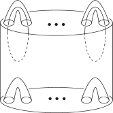
Figure 8. The extended cobordism $(\hat{E},s,\lambda_{\mathcal{A}}\oplus\lambda_{\mathcal{A}})$ containing a framed link $\hat{L}$. If we do extended surgery along $\hat{L}$, we get a fundamental domain $E$. If, instead, we color $\hat{L}$ by $\omega$, we obtain another cobordism $E^{\prime}$.

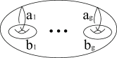
Figure 9. A surface in standard position.

Proposition 4.5.

The closure of $(\hat{E},s,\lambda_{\mathcal{A}}\oplus\lambda_{\mathcal{A}})$ is $(S^{3}(U),s,0)$, where $U$ is a $0$-framed unknot.

Proof.

It is easy to see that the closure of $\hat{E}$ is $S^{3}(U)$. Then we just need to prove that the weight of the closure is $s$. By the gluing formula and Definition 2.11, we have that the weight on $S^{3}(U)$ is

$$s+0-\mu(\lambda_{E}(\Sigma_{g}\cup\bar{\Sigma}_{g}),\lambda(\Sigma_{g}\cup\bar{\Sigma}_{g}),\lambda_{\Sigma_{g}\times[0,1]}(\Sigma_{g}\cup\bar{\Sigma}_{g})).$$

Now let

$$H_{1}(\Sigma_{g})=<a_{1},\cdots,a_{g},b_{1},\cdots,b_{g}>,H_{1}(\bar{\Sigma}_{g})=<a^{\prime}_{1},\cdots,a^{\prime}_{g},b^{\prime}_{1},\cdots,b^{\prime}_{g}>.$$

Then

$$\lambda_{E}(\Sigma_{g}\cup\bar{\Sigma}_{g}) = i_{\Sigma_{g}\cup\bar{\Sigma}_{g},E}^{-1}(0)$$

$$= \{(x,y)\mid x\in<a_{1},\cdots,a_{g}>,y\in<b^{\prime}_{1},\cdots,b^{\prime}_{g}>\}.$$

$$\lambda_{\Sigma_{g}\times[0,1]}(\Sigma_{g}\cup\bar{\Sigma}_{g}) = i_{\Sigma_{g}\cup\bar{\Sigma}_{g},\Sigma_{g}\times[0,1]}^{-1}(0)$$

$$= <(a_{i},-a^{\prime}_{i}),(b_{i},-b^{\prime}_{i})\mid i=1,\cdots,g>.$$

$$\lambda(\Sigma_{g}\cup\bar{\Sigma}_{g}) = \lambda_{\mathcal{A}}\oplus\lambda_{\mathcal{A}}$$

$$= \{(x,y)\mid x\in<a_{1},\cdots,a_{g}>,y\in<a^{\prime}_{1},\cdots,a^{\prime}_{g}>\}$$

So

$$\lambda(\Sigma_{g}\cup\bar{\Sigma}_{g})+\lambda_{E}(\Sigma_{g}\cup\bar{\Sigma}_{g})$$

$$= \{(x,y)\mid x\in<a_{1},\cdots,a_{g}>,y\in<a^{\prime}_{1},\cdots,a^{\prime}_{g}>+<b^{\prime}_{1},..,b^{\prime}_{g}>\}$$

$$= \{(x,y)\mid x\in<a_{1},\cdots,a_{g}>,y\in H_{1}(\bar{\Sigma}_{g})\}.$$

Therefore,

$$\lambda_{\Sigma_{g}\times[0,1]}(\Sigma_{g}\cup\bar{\Sigma}_{g})\cap[\lambda(\Sigma_{g}\cup\bar{\Sigma}_{g})+\lambda_{E}(\Sigma_{g}\cup\bar{\Sigma}_{g})]$$

$$= <(a_{i},-a^{\prime}_{i})\mid i=1,\cdots,g>.$$

It is easy to see that the bilinear form defined in [W] is identically $0$ on $<(a_{i},-a^{\prime}_{i})\mid i=1,\cdots,g>$. So we have

$$\mu(\lambda_{E}(\Sigma_{g}\cup\bar{\Sigma}_{g}),\lambda(\Sigma_{g}\cup\bar{\Sigma}_{g}),\lambda_{\Sigma_{g}\times[0,1]}(\Sigma_{g}\cup\bar{\Sigma}_{g}))=0.$$

Then we get the conclusion. ∎

Proposition 4.6.

Let $(E,s,\lambda_{\mathcal{A}}\oplus\lambda_{\mathcal{A}})$ be the result of extended surgery along the embedded link $\hat{L}$ in $(\hat{E},s,\lambda_{\mathcal{A}}\oplus\lambda_{\mathcal{A}})$ constructed as above starting with a standard surgery presentation diagram for $((M,r),\chi)$. $(E,s,\lambda_{\mathcal{A}}\oplus\lambda_{\mathcal{A}})$ is a fundamental domain for $((M,r),\chi)$.

Proof.

The closure of $(E,s,\lambda_{\mathcal{A}}\oplus\lambda_{\mathcal{A}})$ can be obtained by performing extended surgery on the closure of $(\hat{E},s,\lambda_{\mathcal{A}}\oplus\lambda_{\mathcal{A}})$. This uses the commutative property of gluing discussed in [GM2]. Thus the closure of $E$ is diffeomorphic to $M$, and by [GM2, Lemma 2.2], we see that the closure of $(E,s,\lambda_{\mathcal{A}}\oplus\lambda_{\mathcal{A}})$ has weight $r$. ∎

.

Proposition 4.7.

Let $(E^{\prime},s,\lambda_{\mathcal{A}}\oplus\lambda_{\mathcal{A}})$ be the extended cobordism obtained by coloring the link $\hat{L}$ in $(\hat{E},s,\lambda_{\mathcal{A}}\oplus\lambda_{\mathcal{A}})$ by $\omega$. The SSE class $\mathcal{Z}((M,r),\chi)$ is given by

$$Z(E^{\prime},s,\lambda_{\mathcal{A}}\oplus\lambda_{\mathcal{A}}).$$

Proof.

The equality $Z(E,s,\lambda_{\mathcal{A}}\oplus\lambda_{\mathcal{A}})=Z(E^{\prime},s,\lambda_{\mathcal{A}}\oplus\lambda_{\mathcal{A}})$ follows from the surgery axiom [GM2, Lemma 11.1] for extended surgery. ∎

5. The relation between the Turaev-Viro endomorphism and the tangle endomorphism.

In this section, we will prove the following theorem.

Theorem 5.1.

If $((M,r),\chi)$ is an extended $3$-manifold with an infinite cyclic covering having a surgery presentation $(D_{0},L,s)$ in standard form, then $\mathcal{Z}((M,r),\chi)=Z(D_{0},L,s)$.

Proof.

For simplicity, we indicate the proof in case that $((M,r),\chi)$ does not have a colored trivalent graph. The argument may easily be adapted to the more general case.

We obtain a tangle $\hat{L}_{n}$ from the surgery presentation $(D_{0},L,s)$, and we place black dots on segments in the top part. We will directly compute two matrices for these two endomorphisms with respect to some bases.

Step 1: Compute the entry for the Turaev-Viro endomorphism. We will use the basis in [BHMV2] for $V(\Sigma_{g})$, where $\Sigma_{g}$ is genus $g$ surface. Specifically we choose our spine to be a lollipop graph, as in [GM1]. We show one example of elements as in Figure 10.

Figure 10. An example of elements in the basis for $V(\Sigma_{g})$ constructed in [BHMV2].

Using the method employed in [G2, §8], we can compute the entries of the matrix, with respect to this basis by computing the quantum invariants of colored links in a connected sum of $S^{1}\times S^{2}$’s . We have

$$(i_{1},\cdots,i_{g})\text{-}(j_{1},\cdots,j_{g})\text{\ entry of\ }Z((E^{\prime},s,\lambda_{\mathcal{A}}\oplus\lambda_{\mathcal{A}})$$

$$= \frac{\eta\kappa^{s-\sigma(L^{\prime})}<\text{the first diagram in Figure \ref{tventry}}>}{\eta\kappa^{-\sigma(L^{\prime\prime})}<\text{the first diagram in Figure \ref{JS}}>}.$$

where $L^{\prime}$ as in Figure 11 and $L^{\prime\prime}$ as in Figure 12.

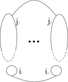
Figure 11. $L^{\prime}$ is consisted of components colored with $\omega$.

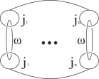
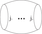
Figure 12. $L^{\prime\prime}$ is consisted of components colored with $\omega$.

By using fusion and Lemma 6 in [L2] and the fact that

$$\sigma(L^{\prime})=\sigma(L^{\prime\prime})=0,$$

we have

$$(i_{1},\cdots,i_{g})\text{-}(j_{1},\cdots,j_{g})\text{\ entry of\ }Z((E^{\prime},-\sigma(L),\lambda_{\mathcal{A}}\oplus\lambda_{\mathcal{A}})$$

$$= \frac{\eta\kappa^{s}\eta^{n}\Delta_{j_{1}}\cdots\Delta_{j_{n}}<U(\omega)>^{n}<\text{the second diagram in Figure \ref{tventry}}>}{\eta<U(\omega)>^{n}<\text{the second diagram in Figure \ref{JS}}>}$$

$$= \frac{\kappa^{s}\eta^{n}\Delta_{j_{1}}\cdots\Delta_{j_{n}}<\text{the second diagram in Figure \ref{tventry}}>}{<\text{the second diagram in Figure \ref{JS}}>}$$

where $U(\omega)$ is the $0$-framing unknot colored with $\omega$.

Step 2: Compute the entry for tangle endomorphism.

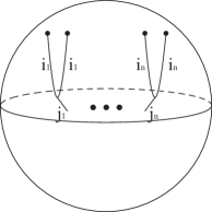
Figure 13. Elements in a basis for ${V(S^{2};2n)}$ which do not automatically vanish under $Z(\hat{L}_{n})$ have this form.

By gluing the tangle in $(S^{2}\times I,s)$ to the basis element in Figure 13, we can see that

$$(i_{1},\cdots,i_{g})\text{-}(j_{1},\cdots,j_{g})\text{\ entry of\ }Z(\hat{L}_{n})$$

$$= \frac{\kappa^{s}\eta^{n}\Delta_{j_{1}}\cdots\Delta_{j_{n}}<\text{the second diagram in Figure \ref{tventry}}>}{<\text{the second diagram in Figure \ref{JS}}>}$$

for $(i_{1},\cdots,i_{n},j_{1},\cdots,j_{n})$ a legal coloring, and is zero otherwise.

Step 3: The two matrices are strong shift equivalent. By above discussion, it is easy to see that if the matrix for Turaev-Viro endomorphism is $X$, then a matrix for tangle endomorphism is the block matrix $\begin{bmatrix}X&0\\ 0&0\end{bmatrix}.$ We see that this block matrix is strong shift equivalent to $X$ by Proposition 2.22. ∎

6. Proof of Theorem 3.7

Lemma 6.1.

The transformation process in Proposition 2.19 does not change the strong shift equivalent class of the tangle endomorphism.

Proof.

A small extended Kirby-$1$ move adds a $\pm 1$ framed $\omega$ to all the different decorations of $\mathcal{T}^{n}_{n}$ which go into the definition of $Z(\mathcal{T}^{n}_{n})$. This would seem to multiply $Z(\mathcal{T}^{n}_{n})$ by $\kappa^{\pm 1}$. But a small extended Kirby-$1$ move also changes $\sigma(L)$ by $\pm 1,$ and thus changes the weight $s$ of $S^{2}\times I\supset\mathcal{T}^{n}_{n}$ by $\mp 1$. These two effects of the move cancel out and $Z(\mathcal{T}^{n}_{n})$ is unchanged. The small Kirby-$2$ moves preserves all the summands of $Z(\mathcal{T}^{n}_{n})$, by a well known handle slide property of $\omega.$ See [KL, Lemma 21] for instance. Two tangles related by a $D_{0}$ move are obtained by cutting $S^{2}\times S^{1}$ along two different $S^{2}$’s. Suppose if we cut $S^{2}\times S^{1}$ along $S_{0}=S^{2}\times\{p_{0}\}$, we obtain a tangle $\hat{L}_{n}$. If we cut along $S_{1}=S^{2}\times\{p_{1}\}$, we obtain a tangle $\hat{L}^{\prime}_{m}$. By those two cutting, we obtain two homomorphisms

$$Z(\hat{L}_{n}):{V(S_{1})}\rightarrow{V(S_{1})}$$

and

$$Z(\hat{L}^{\prime}_{m}):{V(S_{0})}\rightarrow{V(S_{0})}.$$

Now suppose we cut $S^{2}\times S^{1}$ along $S^{2}\times\{p_{0}\}$ and $S^{2}\times\{p_{1}\}$, we get a $(n,m)$-tangle in $(S^{2}\times I,0)$, denoted by $T_{1}$, and a $(m,n)$-tangle, denoted by $T_{2}$. $T_{1}$ defines a homomorphism

$$Z(T_{1}):{V(S_{1})}\rightarrow{V(S_{0})},$$

and $T_{2}$ defines a homomorphism

$$Z(T_{2}):{V(S_{0})}\rightarrow{V(S_{1})}.$$

It is easy to see that

$$Z(\hat{L}_{n})=Z(T_{2})Z(T_{1}),$$

and

$$Z(\hat{L}^{\prime}_{m})=Z(T_{1})Z(T_{2}).$$

Therefore, $Z(\hat{L}_{n})$ is strong shift equivalent to $Z(\hat{L}^{\prime}_{m}).$ ∎

Lemma 6.2.

Suppose we have two surgery presentations $(D_{0},L_{1},s_{1},G_{1})$ and $(D_{0},L_{2},s_{2},G_{2})$ for $(M,r,\chi,G^{\prime})$ in standard form, then

$$Z(D_{0},L_{1},s_{1},G_{1})=Z(D_{0},L_{2},s_{2},G_{2}).$$

Proof.

This easily follows from Propositions 5.1. ∎

Proof of Theorem 3.7.

By Proposition 2.19, and Lemma 6.1, we can transform $(D_{0},L_{1},s_{1},G_{1})$ and $(D_{0},L_{2},s_{2},G_{2})$ so that they are standard without changing the SSE class of their induced tangle endomorphism. Then the result follows from Lemma 6.2. ∎

7. Colored Jones polynomials and Turaev-Viro endomorphisms

In this section, we assume, for simplicity, that $p$ is odd. Similar formulas could be given for $p$ even, by the same methods. We let $J(K,i)$ denote the bracket evaluation of a knot diagram of $K$ with zero writhe colored $i$ at a primitive $2p$th root of unity $A$. Letting $U$ denote the unknot, we have that $J(U,i)=\Delta_{i}$. In particular, $J(U,1)=-A^{2}-A^{-2}$. This is one normalization of the colored Jones polynomial at a root of unity.

Remark 7.1.

Using [BHMV1, Lemma 6.3], we have that:

$$J(K,i+p)=-J(K,i)\text{, and }J(K,i+(p-1)/2)=J(K,-i+(p-3)/2).$$

Without losing information, we can restrict our attention to $J(K,2i)$ for $0\leq i\leq(p-3)/2.$ For other $c$, $J(K,c)=\pm J(K,2i)$ for some $0\leq i\leq(p-3)/2,$ using the above equations.

Let $(S^{3}(K),i,j,0))$ denote 0-framed surgery along an oriented knot $K$ in $S^{3}$ decorated with a meridian to $K$ colored $i$ and a longitude little further away from $K$ colored $j$ and equipped with the weight zero. Let $\chi$ be the homomorphism from $H_{1}(M)$ to ${\mathbb{Z}}$ which sends a meridian to one. Let ${\operatorname{TV}}(K,i,j)$ denote the SSE class of the Turaev-Viro endomorphism $\mathcal{Z}(S^{3}(K),i,j,0)),\chi)$. The vector space associated to a 2-sphere with just one colored point which is colored by an odd number is zero. Using this fact, and a surgery presentation, one sees that

$${\operatorname{TV}}(K,i,j)=0\text{ if $i$ is odd.}$$

The second author studied ${\operatorname{TV}}(K,i,0)$ [G1, G2]. The idea of adding the longitude with varying colors is due to Viro [V1, V2]. The least interesting case, of this next theorem, when $j=0$ already appeared in [G1, Corollary 8.3].

Theorem 7.2 (Viro).

For $0\leq j\leq p-2$,

$$J(K,j)=\sum_{i=0}^{(p-3)/2}\Delta_{2i}{\operatorname{Trace}}({\operatorname{TV}}(K,2i,j)).$$

Proof.

One has that $0$-framed surgery along $K$ with the weight zero is the result of extended surgery of $S^{3}$ with weight zero along a zero-framed copy of $K$. If we add then a zero-framed meridian of $K$ to this framed link description, we undo the surgery along $K$ and we get back an extended surgery description of $S^{3}$, also with weight zero. A longitude to $K$ colored $j$ and placed a little outside the meridian will go to a longitude of $K$ colored $j$ in $S^{3}$, which is of course isotopic to $K$. But adding a zero-framed meridian to the framed link changes $<\ >_{p}$ in the same way as cabling by $\omega=\eta\sum_{i=0}^{(p-3)/2}\Delta_{2i}e_{2i}$. If we cable the meridian of $K$ by $e_{2i}$ instead of by $\omega$, and calculate $<\ >_{p}$, we get

$$<(S^{3}(K),2i,j,0)>_{p}={\operatorname{Trace}}({\operatorname{TV}}(K,2i,j)),$$

by the trace property of TQFT [BHMV2, 1.2]. Thus

$$<S^{3}\text{ with $K$ colored $j$}>=\eta\sum_{i=0}^{(p-3)/2}\Delta_{2i}{\operatorname{Trace}}({\operatorname{TV}}(K,2i,j)).$$

Dividing by $\eta$ yields the result. ∎

Thus the colored Jones is determined by the traces of the ${\operatorname{TV}}(K,2i,j).$ The next theorem shows that the $J(K,j)$ determine the traces of the ${\operatorname{TV}}(K,2i,j)$.

Theorem 7.3.

For $0\leq i,j\leq(p-3)/2$,

$${\operatorname{Trace}}({\operatorname{TV}}(K,2i,2j))=\eta^{2}\sum_{k=0}^{(p-3)/2}\sum_{l=|k-j|}^{k+j}\Delta_{(2k+1)(2i+1)-1}J(K,2l).$$

More generally :

$${\operatorname{Trace}}({\operatorname{TV}}(K,2i,j))=\eta^{2}\sum_{k=0}^{(p-3)/2}\sum_{\begin{matrix}l=|2k-j|\\ l\equiv j\mod 2\end{matrix}}^{2k+j}\Delta_{(2k+1)(2i+1)-1}J(K,l).$$

.

Proof.

By the trace property of TQFT,

$${\operatorname{Trace}}({\operatorname{TV}}(K,2i,2j))=<(S^{3}(K),2i,2j)>_{p}.$$

Direct calculation of $<(S^{3}(K),2i,2j)>_{p}$ from the definition yields $\eta$ times the bracket evaluation of $K$ cabled by $\omega$ together with the meridian colored $2i$ and the longitude further out colored $2j$. These skeins all lie in a regular neighborhood of $K$ with framing zero. These skeins can then be expanded as a linear combination of the core of this solid torus with different colors.

The operation of encircling an arc colored $2k$ with loop colored $2j$ in the skein module of a local disk has the same effect as multiplying the arc by $\Delta_{(2k+1)(2j+1)-1}/\Delta_{2k}$ by [L1, Lemma 14.2]. Note the idempotents $f_{k}$ are only defined for $0\leq k\leq(p-2).$ It is well known that the $e_{k}$ satisfy a recursive formula which can be used to extend the definition of $e_{k}$ for all $k\geq 0$. This is given [BHMV1] as follows: $e_{0}=1$, $e_{1}$ is the zero framed core of a solid standard solid torus, and $e_{k}=ze_{k-1}-e_{k-2}$. In the skein module of a solid torus, we have $e_{2k}.e_{2j}=\sum_{l=|k-j|}^{k+j}e_{2l}$. Using these rules, the expansion can be worked out to be

$$\eta\sum_{k=0}^{(p-3)/2}\sum_{l=|k-j|}^{k+j}\Delta_{(2k+1)(2i+1)-1}e_{2l}.$$

The second equation is worked out in a similar way. ∎

Notice that, in the summation on the right of the first equation in Theorem 7.3, $J(K,2l)$ for $l>{(p-3)/2}$ sometimes appears. This can be rewritten using Remark 7.1 as $J(K,2j)$ for $j\leq{(p-3)/2}$.

We remark that using [G4, Corollary 2.8], one can see that the Turaev-Viro polynomials of ${\operatorname{TV}}(K,i,j)$ will have coefficients in a cyclotomic ring of integers, if $p$ is an odd prime or twice an odd prime.

8. Examples

In this section, we wish to illustrate with some concrete examples how to calculate the ${\operatorname{TV}}(K,i,j)$ using tangle morphisms in the case $p=5$ (which is the first interesting case). For both examples, we check our computation against an identity from the previous section.

The first example is the $k$-twist knot with meridian colored $0$ or $2$ and longitude colored $2$. We then verify directly the equation in Theorem 7.2 for the case $p=5$, $j=2$, and $K$ is the $k$-twist knot.

The second example we study is the knot $6_{2}$ with the meridian and longitude uncolored. We work out, using tangle morphisms, the traces of the Turaev-Viro endomorphism. We then verify the equation in Theorem 7.3 when $p=5$, $i=j=0$, and $K=6_{2}$.

We pick an orthogonal basis for the module associated with a 2-sphere with some points, and use this basis to work out the entries on the matrix for the tangle endomorphism coming from a surgery presentation. The bases are represented by colored trees in the 3-ball which meet the boundary in the colored points as in Figure 13. Here we will refer to these colored trees as basis-trees. Each entry is obtained as a certain quotient. The numerator is the evaluation as a colored fat graph in $S^{3}$ obtained from the tangle closed off with the source basis-tree at the bottom and the target basis-tree at the top. The denominator is the quotient as the evaluation of the double of the target basis element. In both examples, we use a surgery presentation, with one surgery curve with framing $+1$. Thus the initial weight of $S^{3}$, denoted $s$ above, should be $-1$, so the weight of $S^{3}$ after the surgery is zero. This puts a factor of $\kappa^{-1}$ in front of the tangle endomorphism. There is also a uniform factor of $\eta$ coming from the single black dot on a strand with two endpoints. We put this total factor of $\kappa^{-1}\eta$ in front. We also have $\Delta_{i}$ prefactors where $i$ is the color of the strand with the black dot, and these factor vary from entry to entry.

To simplify our formulas, when $p=5$, we use ${\operatorname{Tet}}$ to abbreviate ${\operatorname{Tet}}(2,2,2,2,2,2)$, $\Delta$ to abbreviate $\Delta_{1}=\Delta_{2}$ and $\Theta$ to denote $\Theta(2,2,2)$.

8.1. The Turaev-Viro endomorphism and the colored Jones polynomial of the $k$-twist knot.

A tangle $T$ for the $k$-twist knot with meridian and longitude is given in Figure 14.

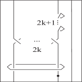
Figure 14. Surgery presentation of $k$-twist knot with meridian and longitude. The straight line is from the meridian and the circle is from the longitude. We have also chosen a position for the black dot.

If we denote by $T_{0}$ the tangle $T$ with meridian colored by $0$ and longitude colored by $2$, and let $S$ denote a 2-sphere with two uncolored points, then we obtain a map

$${\operatorname{TV}}(K,0,2)=Z(T_{0}):{V(S)}\rightarrow{V(S)}.$$

By using the trivalent graph basis in [BHMV2],

$${V(S)}=\text{Span}<a_{1},a_{2}>,$$

where $a_{1},a_{2}$ are as in Figure 15.

Figure 15. A basis for ${V(S)}$ where $S$ is a 2-sphere with two uncolored points

With respect to this basis, we have

$${\operatorname{TV}}(K,0,2)=\kappa^{-1}\eta\begin{bmatrix}\Delta&\Delta^{3}\\ \Delta A^{16k+8}&\Delta(A^{8}+\Delta A^{8k+8}).\end{bmatrix}$$

We follow the convention that the columns of the matrix for a linear transformation with respect to a basis are given the images of that basis written in terms of that basis. The characteristic polynomial of this matrix (i.e. the Turaev-Viro polynomial) has coefficients in ${\mathbb{Z}}[A].$

If we denote by $T_{2}$ the tangle $T$ with meridian colored by $2$ and longitude colored by $2$, and let $S$ denote a 2-sphere with two uncolored points and one point colored $2$, then we obtain a map

$${\operatorname{TV}}(K,2,2)=Z(T_{2}):{V(S)}\rightarrow{V(S)}.$$

By using the trivalent graph basis in [BHMV2],

$${V(S)}=\text{Span}<b_{1},b_{2},b_{3}>,$$

where $b_{1},b_{2},b_{3}$ are as in Figure 16.

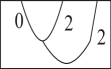
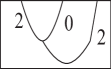
Figure 16. A basis for ${V(S)}$ where $S$ is a 2-sphere with two uncolored points and one point colored 2

With respect to this basis, we have

$$TV(K,2,2)=\kappa^{-1}\eta\begin{bmatrix}-(\frac{A^{8}}{\Delta}+\frac{A^{8k+8}\Delta{\operatorname{Tet}}}{\Theta^{2}})&0&0\\ 0&0&0\\ 0&0&0\end{bmatrix}\ .$$

By Proposition 2.22, we also have $TV(K,2,2)=\begin{bmatrix}-\kappa^{-1}\eta(\frac{A^{8}}{\Delta}+\frac{A^{8k+8}\Delta{\operatorname{Tet}}}{\Theta^{2}})\end{bmatrix}\ .$ This last expression lies in ${\mathbb{Z}}[A]$ for all $k$. One has that:

$${\operatorname{Trace}}(TV(K,0,2))+\Delta{\operatorname{Trace}}(TV(K,2,2))$$

$$= \kappa^{-1}\eta\Delta(1+A^{8}+\Delta A^{8k+8})-\kappa^{-1}\eta\Delta(\frac{A^{8}}{\Delta}+\frac{A^{8k+8}\Delta{\operatorname{Tet}}}{\Theta^{2}}).$$

Moreover, we used recoupling theory as in [MV, KL, L1] to calculate the $2$-colored Jones polynomial of $k$-twist knot directly to obtain:

$$J(K,2)=-\frac{A^{4}}{\Delta}+(1+\frac{\Delta^{2}{\operatorname{Tet}}}{\Theta^{2}A^{8}})A^{8k}$$

We used Mathematica to verify that the two calculations agree for all $k$.

8.2. The Turaev-Viro endomorphism of $6_{2}$ and quantum invariant of $S^{3}(6_{2})$.

In this section, we will compute the Turaev-Viro endomorphism and quantum invariant of $S^{3}(6_{2})$ when $A$ is a primitive $10$th root of unity and verify that the trace of the Turaev-Viro endomorphism equals to quantum invariant. By $6_{2}$, we mean the knot as pictured in [CL], which is the mirror image of the knot as pictured in [L1, R1]. A tangle $T$ for $S^{3}(6_{2})$ is as in Figure 17.

Figure 17. Tangle for $S^{3}(6_{2})$, with a choice for the position for the black dot.

So we obtain a map

$${\operatorname{TV}}(6_{2},0,0)=Z(T):{V(S)}\rightarrow{V(S)}.$$

where $S$ is a 2-sphere with four uncolored points. We use a trivalent graph basis in [BHMV2] for ${V(S)}$ as in Figure 18.

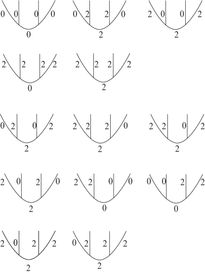
Figure 18. A basis for ${V(S)}$, where $S$ is a 2-sphere with four uncolored points.

With respect to this basis, we can obtain a $13\times 13$ matrix, which is in the strong shift equivalence class of the Turaev-Viro endomorphism. However, by Proposition 2.22 applied twice in succession, it is enough to consider the minor given by the first five rows and columns. We thus obtain a $5\times 5$ matrix:

$${\operatorname{TV}}(6_{2},0,0)=\kappa^{-1}\eta\begin{pmatrix}1&0&\Delta^{2}&0&0\\ A^{2}&0&\Delta(A^{3}+A)&0&0\\ 0&A^{4}&0&\Delta&A^{2}\Theta\\ 0&\frac{A^{8}}{\Delta}&0&A^{8}&\frac{A^{8}\Theta}{\Delta}\\ 0&\frac{\Delta A^{2}}{\Theta}&0&\frac{\Delta^{2}}{\Theta}&\Delta(1-A^{6}+A^{8}+\frac{(A^{4}-A^{6})\Delta{\operatorname{Tet}}}{\Theta^{2}})\end{pmatrix}.$$

The Turaev-Viro polynomial (at $p=5$) is the characteristic polynomial of the above matrix, namely:

$$x^{5}+\left(A^{3}+A-1\right)x^{4}+\left(-A^{3}-A^{2}-A\right)x^{3}+\left(A^{2}+A+1\right)x^{2}+\left(A^{3}-A^{2}-1\right)x-A^{3}.$$

We also note that

$${\operatorname{Trace}}({\operatorname{TV}}(6_{2},0,0))=1-A-A^{3}.$$

The left hand side of the first equation in Theorem 7.3, with $i=j=0$, and $K=6_{2}$ is by definition, the quantum invariant of $S^{3}(6_{2})$. The right hand side is, by direct computation:

$$\eta^{2}(J({6_{2}},0)\Delta_{0}+J({6_{2}},2)\Delta_{2}=\eta^{2}(1+\Delta(-A^{-2}+A^{2}-A^{8}-A^{6}))=1-A-A^{3}$$

Therefore, we verify a case of the first equation in Theorem 7.3.

References

- [AB] H. Achir, C. Blanchet, On the computation of the Turaev-Viro module of a knot, Journal Of Knot Theory and Its Ramifications. Vol 7, No. 7(1998), 843-856.
- [BHMV1] C. Blanchet, N. Habegger, G. Masbaum, P. Vogel, Three-manifolds invariants derived from the Kauffman bracket, Topology 31 (1992), 685–699
- [BHMV2] C. Blanchet, N. Habegger, G. Masbaum, P. Vogel, Topological quantum field theories from the Kauffman bracket, Topology 34 (1995), 883–927.
- [BH] M.Boyle, D.Handelman, Algebraic shift equivalence and primitive matrices, Trans. Amer. Math. Soc. 336 (1993), no. 1, 121–149.
- [CL] J. C. Cha and C. Livingston, KnotInfo: Table of Knot Invariants, http://www.indiana.edu/~knotinfo, January 31, 2012.
- [G1] P. M. Gilmer, Invariants for one-dimensional cohomology classes arising from TQFT, Topology And Its Applications 75 (1997), 217-259.
- [G2] P. M. Gilmer, Turaev-Viro modules of satellite knots, KNOTS ’96 (Tokyo).
- [G3] P. M. Gilmer, Topological quantum field theory and strong shift equivalence, Canad. Math. Bull. 42 (1999) 190-197.
- [G4] P.M. Gilmer, Integrality for TQFTs, Duke Math. J. 125 (2004) 389–413.
- [GM1] P. M. Gilmer, G. Masbaum, Integral Lattices in TQFT, Annales Scientifiques de l’Ecole Normale Superieure, 40, (2007), 815–844
- [GM2] P. M. Gilmer, G. Masbaum, Maslov index, lagrangians, mapping class groups and TQFT, arXiv:0912.4706v3. to appear in Forum Mathematicum
- [KL] L.Kauffman, S. Lins, Temperley-Lieb recoupling theory and invariants of 3-manifolds. Annals of Mathematics Studies, 134. Princeton University Press, Princeton, NJ, 1994.
- [K] R. C. Kirby, A calculus for framed links, Invent. Math. 45 (1978), 395-401.
- [L1] W.B.R., Lickorish, An introduction to knot theory, Graduate Texts in Mathematics, 175, Springer-Verlag, New York, 1997.
- [L2] W.B.R., Lickorish, The skein method for three-manifold invariants, J. Knot Theory Ramifications 2 (1993), no. 2, 171–194
- [LM] D. Lind, B. Marcus, Introduction to Symbolic Dynamics and Coding, Cambridge University Press, (1995)
- [MV] G.Masbaum, P. Vogel, 3-valent graphs and the Kauffman bracket, Pacific J. Math. 164 (1994), no. 2, 361–381
- [O1] T. Ohtsuki, Equivariant quantum invariants of the infinite cyclic covers of knot complements, Intelligence of low dimensional topology 2006, 253-262, Ser. Knots Everything 40, World Sci. Publ., Hackensack, NJ, 2007.
- [O2] T. Ohtsuki, Invariants of knots derived from equivariant linking matrices of their surgery presentations. Internat. J. Math. 20 (2009), no. 7, 883–913.
- [R1] D. Rolfsen, A surgical view of Alexander’s polynomial. Geometric topology (Proc. Conf., Park City, Utah, 1974), pp. 415–423. Lecture Notes in Math., Vol. 438, Springer, Berlin, 1975.
- [R2] D. Rolfsen, Knots and links, Corrected reprint of the 1976 original. Mathematics Lecture Series, 7. Publish or Perish, Inc., Houston, TX, 1990.
- [T] V. Turaev, Quantum invariants of knots and 3-manifolds. Second revised edition. de Gruyter Studies in Mathematics, 18. Walter de Gruyter Co., Berlin, 2010.
- [TV] V. Turaev, O. Viro, Lecture by Viro at Conference on Quantum Topology: Kansas State University, Manhattan, Kansas, March 1993
- [V1] O. Viro, conversation with P. Gilmer, January 2011
- [V2] O. Viro, Elevating link homology theories and TQFT’s via infinite cyclic coverings, Lecture by Viro at Swiss Knots May 2011, http://www.math.toronto.edu/~drorbn/SK11/
- [W] C. Wall, Non-additivity of the signature, Invent. Math. 7 (1969), 269-274.
- [Wa1] K. Walker, Topological quantum field theories and minimal genus surfaces, Lecture, International Conference on Knots 90, Osaka, Japan, August 1990
- [Wa2] K. Walker, On Witten’s 3-manifold invariants, Preliminary Version, 1991 http://canyon23.net/math/
- [Wag] J. Wagoner, Strong shift equivalence theory and the shift equivalence problem. Bull. Amer. Math. Soc. 36 (1999), no. 3, 271–296.