Entanglement amplification via local weak measurements

Abstract

We propose a measurement-based method to produce a maximally-entangled state from a partially-entangled pure state. Our goal can be thought of as entanglement distillation from a single copy of a partially-entangled state. The present approach involves local two-outcome weak measurements. We show that application of these local weak measurements leads to a probabilistic amplification of entanglement. In addition, we examine how the probability to find the maximally-entangled state is related to the entanglement of the input state. We also study the application of our method to a mixed initial state. We show that the protocol is successful if the separable part of the mixed initial state fulfils certain conditions.

1 Introduction

Measurements on quantum systems as well as the coherent manipulation via unitary operations are key ingredients to the implementation of interesting quantum state-engineering protocols. An essential feature of quantum measurements [1, 2, 3, 4] is that these significantly affect the static and dynamic properties of the system. This allows phenomena not predicted by classical mechanics, such as the quantum Zeno effect [5, 6].

Many measurement-based schemes have been studied including: one-way quantum computation [7], protection or recovery of a quantum state in a noisy channel [8, 9, 10, 11], preparation of an entangled state [12], and measurement-based quantum control [13, 14]. Among these approaches, the use of weak (or general) measurements has recently drawn considerable attention. General measurements are the generalization of von Neumann measurements and are associated with a positive-operator valued measure (POVM) [1, 2, 3]. Their influence on a quantum system is, in general, more moderate than von Neumann measurements. Thus, in some cases, the amount of information extracted using weak measurements can be tunable. This feature is useful to implement quite interesting quantum protocols, such as reversing measurements [15, 16] and weak-value measurements [17, 18].

In this paper, we study a method to prepare a maximally-entangled state from a pure initial state using weak measurements. Our goal can be considered to be entanglement distillation with a single copy of a partially-entangled state. The present approach involves local two-outcome weak measurements. We show that the application of local weak measurements leads to a probabilistic amplification of the entanglement. Furthermore, we examine the relationship of our scheme with an entanglement-concentration protocol [19, 20]. The present study shows several interesting roles of a weak measurement.

The paper is organized as follows. First, we explain our setting in section 2. Section 3 is the main part of this paper. We propose a method to produce a maximally-entangled state from a partially-entangled pure state with the application of local weak measurements. The key idea is to tune the measurement strength at each measurement step. Our approach developed in section 3 assumes that the input state is a pure state. In order to consider more realistic situations, we examine the case when the input state is a mixed state in section 4. Then, we find that the method for a pure state still leads to entanglement amplification if the separable part of the initial mixed state fulfills certain conditions. Furthermore, we discuss the extendability of this approach in section 5. Section 6 is devoted to a summary of the results.

2 Setting

2.1 Linear entropy

Let us consider a bipartite system composed of a two- and a $d$-level system ($d\geq 2$). The two-level system is called system A, while the $d$-level one is called system B. We will apply some operations only to system A and never touch system B. Since system A is a single-qubit, the treatment of control processes is rather simple. We have a pure state $|\psi\rangle$ in this composite system,

$$|\psi\rangle=\alpha|0\rangle|\phi_{0}\rangle+\beta|1\rangle|\phi_{1}\rangle,\quad|i\rangle\in\mathbb{C}^{2},\quad|\phi_{i}\rangle\in\mathbb{C}^{d},$$ (1)

with $\alpha^{2}+\beta^{2}=1$, $\alpha\geq 0$, $\beta\geq 0$, $\langle i|j\rangle=\delta_{ij}$, and $\langle\phi_{i}|\phi_{j}\rangle=\delta_{ij}$ ($i,j=0,1$). We also note that $\alpha$ and $\beta$ are real parameters. Mathematically, we can always find this form of a vector with the Schmidt decomposition [3]. The quantum correlation of $|\psi\rangle$ is characterized by the purity of the reduced density matrix $\rho_{\rm A}=\mbox{Tr}\,_{\rm B}(|\psi\rangle\langle\psi|)$, as seen in, e.g., [4]. We consider the linear entropy

$$S(\psi)=2[1-\mbox{Tr}\,_{\rm A}(\rho_{\rm A}^{2})]=4\alpha^{2}\beta^{2}.$$ (2)

When $S(\psi)=0$, we find that either $\alpha=0$ or $\beta=0$. Hence, there is no correlation between the two subsystems. In contrast, when $S(\psi)>0$, $|\psi\rangle$ has a quantum correlation, i.e., entanglement. In particular, $S(\psi)$ takes its maximum value $1$ when $\rho_{\rm A}$ is a maximally-mixed state (i.e., when $\alpha=\beta$). This indicates that we have a maximally-entangled state. Thus, the linear entropy $S(\psi)$ can be regarded as an entanglement measure.

2.2 Motivation

Entanglement is one of the key resources of quantum information processing such as quantum teleportation, quantum dense coding, quantum key distribution, and so on [21]. To develop a way to create and protect maximally-entangled states is quite important because most quantum protocols rely on their existence. Thus, an interesting physical issue is that (1) is a partially-entangled state (i.e., $\alpha\neq\beta$ and $\alpha,\beta>0$) and one might desire to amplify its entanglement. Typically, one can encounter such an issue when one tries to create a maximally-entangled state in the presence of experimental imperfections. Our aim is to find an efficient and practical way to transform $|\psi\rangle$ into a maximally-entangled state. The most straightforward way might be to use controlled unitary operators between the two subsystems. Entanglement purification with many copies of $|\psi\rangle$ is also a candidate to accomplish this goal, as seen, e.g., in [21]. However, these methods can be costly, e.g., either requiring properly controlled gates, or preparing a sufficient number of copies, or two-body measurements. Here we wish to propose a simpler method to achieve the same goal. Namely, we want to create a maximally-entangled state from a partially-entangled state using a simpler experimental setting. Thus, we consider the case when one can use only local operations and a single copy of $|\psi\rangle$.

We now illustrate our task more explicitly. Without loss of generality, we assume that $\beta>\alpha$ in (1). Let us consider a completely positive and trace-preserving (CPTP) map [2]

$$\rho_{\rm in}=|\psi\rangle\langle\psi|\mapsto\rho_{\rm out}=\sum_{\ell}\hat{K}_{\ell}|\psi\rangle\langle\psi|\hat{K}_{\ell}^{\dagger}$$ (3)

with a set of linear operator $\hat{K}^{\rm A}_{\ell}$ on $\mathbb{C}^{2}$, $\hat{K}_{\ell}=\hat{K}^{\rm A}_{\ell}\otimes\hat{I}_{d}$ and $\sum_{\ell}\hat{K}_{\ell}^{\dagger}\hat{K}_{\ell}=\hat{I}_{2}\otimes\hat{I}_{d}$. The identity operator on $\mathbb{C}^{2}$ ($\mathbb{C}^{d}$) is denoted by $\hat{I}_{2}$ ($\hat{I}_{d}$). The entanglement of $\rho_{\rm out}$ must be smaller than the entanglement of $\rho_{\rm in}$ because this map is composed of only local operators. However, a portion of $\rho_{\rm out}$, e.g., $\hat{K}_{\ell}|\psi\rangle\langle\psi|\hat{K}_{\ell}^{\dagger}/\mbox{Tr}\,(\hat{K}_{\ell}|\psi\rangle\langle\psi|\hat{K}_{\ell}^{\dagger})$ can be a more strongly entangled state than $\rho_{\rm in}$ [21]. The local map (3) allows entanglement distillation with probability $\mbox{Tr}\,(\hat{K}_{\ell}|\psi\rangle\langle\psi|\hat{K}_{\ell}^{\dagger})$. Thus, the problem reduces to seeking a set of $\hat{K}_{\ell}^{\rm A}$’s and how to apply them.

Our goal can be thought of as entanglement distillation from a single copy of a partially-entangled state. Bennett et al. [19] suggested a scheme to purify a maximally-entangled state from a partially-entangled pure state using local partial-collapse measurements [15], i.e., $\hat{K}_{1}^{\rm A}=\sqrt{p}|1\rangle\langle 1|$ and $\hat{K}_{2}^{\rm A}=|0\rangle\langle 0|+\sqrt{1-p}|1\rangle\langle 1|$, with $0\leq p\leq 1$. Kwiat et al. [20] reported the experimental realization of this scheme. Although one has to discard the quantum state when the outcome is $\hat{K}_{1}^{{\rm A}\,\dagger}\hat{K}_{1}^{\rm A}$, one obtains a maximally-entangled state when the outcome is $\hat{K}_{2}^{{\rm A}\,\dagger}\hat{K}_{2}^{\rm A}$. Several other entanglement distillation procedures have been proposed (e.g., [22]) but using many copies of a partially-entangled state. The demonstration of the methods with two copies of partially-entangled states was reported in, e.g., [23, 24]. The basic setting in this paper is the same as in [19, 20] (i.e., the use of a single copy of a pure state and local measurements). Thus, hereafter, we will use the term “distillation” for describing our protocol although we do not treat a large ensemble of mixed states but just a single copy of a partially-entangled pure state.

We propose a method for entanglement amplification with local weak measurements and a single copy of a partially-entangled pure state. If the measurement is successful, we obtain a maximally-entangled state. We stress that our approach requires a small cost because a lot of copies and two-body measurements are not needed. The type of the weak measurements used in our protocol is different from the one in the proposal by Bennett et al. (so-called Procrutean method) [19], and was demonstrated in, e.g, [17]. Although our approach is similar to the Procrutean method, the present method does not completely destroy entanglement even if the measurement fails. Thus, we can repeatedly apply weak measurements until we obtain a maximally-entangled state. We also remark that when one has a physical system in which the implementation of the weak measurements in [19] is difficult, one can use the present approach as an alternative method for entanglement distillation of a single copy of a pure state.

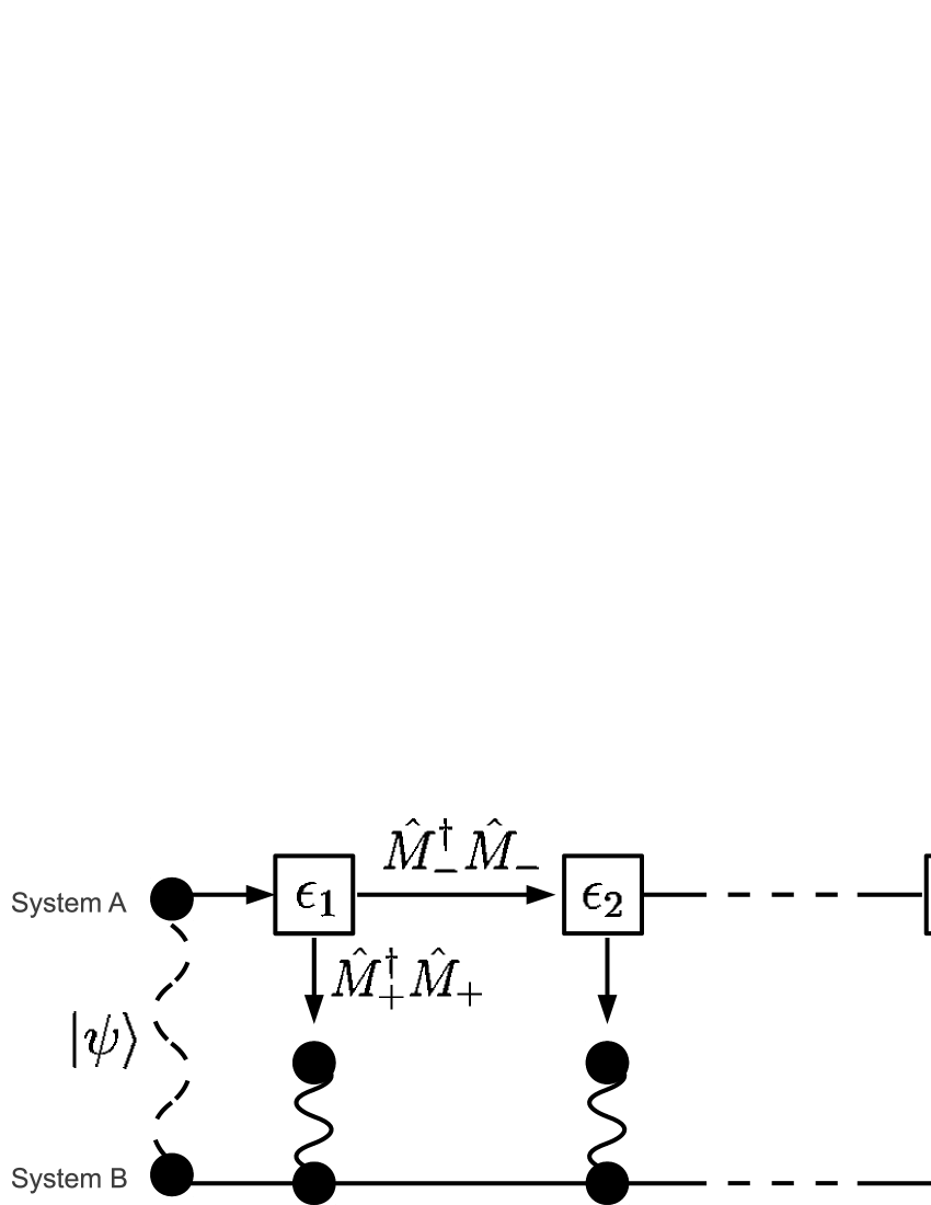
Figure 1: Schematic diagram of our approach to distill a maximally-entangled state from a partially-entangled initial state $|\psi\rangle=\alpha|0\rangle|\phi_{0}\rangle+\beta|1\rangle|\phi_{1}\rangle$. The measurements are performed only on system A. Each box indicates the measurement apparatus with the measurement strength $\epsilon_{n}$ ($n=1,\,2,\,\ldots,N$), see (4). When we obtain the outcome corresponding to $\hat{M}_{+}^{\dagger}\hat{M}_{+}$, we find a maximally-entangled state.

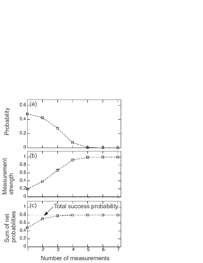
Figure 2: Application of our approach to $\alpha|0\rangle|\phi_{0}\rangle+\beta|1\rangle|\phi_{1}\rangle$ with $\alpha^{2}=0.4$ and $\beta^{2}=0.6$. The horizontal axis is the number of measurements performed. The probability to obtain a maximally-entangled state is shown in (a). The measurement strength is shown in (b). The sum of the net probabilities, which is defined as (12), is shown in (c). The dotted line indicates the total success probability, $2\alpha^{2}=0.8$. See (13) and (17). A higher total success probability could be easily obtained by choosing $2\alpha^{2}$ close to one.

3 Entanglement amplification with local weak measurements

Now we show a method to distill entanglement from a partially-entangled pure initial state. The basic part of the scheme is the weak measurements on system A given by

$$\hat{M}_{\pm}(\epsilon)=\sqrt{\frac{1\pm\epsilon}{2}}|0\rangle\langle 0|+\sqrt{\frac{1\mp\epsilon}{2}}|1\rangle\langle 1|,$$ (4)

$$\hat{M}_{+}^{\dagger}\hat{M}_{+}+\hat{M}_{-}^{\dagger}\hat{M}_{-}=\hat{I}_{2},$$ (5)

with measurement strength $\epsilon$ ($0\leq\epsilon\leq 1$). The set $\{\hat{M}_{\sigma}^{\dagger}\hat{M}_{\sigma}\}_{\sigma=+,-}$ is a POVM [1, 2, 3] on $\mathbb{C}^{2}$. These measurements with tunable $\epsilon$ can be implemented in various physical systems, as seen, e.g., in [17, 25, 29]. We substitute $\hat{M}_{+}(\epsilon)$ and $\hat{M}_{-}(\epsilon)$, respectively, into $\hat{K}^{\rm A}_{1}$ and $\hat{K}^{\rm A}_{2}$ in (3). The resultant state is given by $\rho_{\rm out}=p_{+}|\psi_{+}\rangle\langle\psi_{+}|+p_{-}|\psi_{-}\rangle\langle\psi_{-}|$ with $|\psi_{\pm}\rangle=(\hat{M}_{\pm}\otimes\hat{I}_{d})|\psi\rangle/\sqrt{p_{\pm}}$ and $p_{\pm}=\langle\psi|(\hat{M}_{\pm}^{\dagger}\hat{M}_{\pm}\otimes\hat{I}_{d})|\psi\rangle$. The important point here is that $|\psi_{+}\rangle$ is a maximally-entangled state when $\alpha^{2}(1+\epsilon)/2=\beta^{2}(1-\epsilon)/2$. Assuming that $\beta>\alpha$, we find that the parameter $\epsilon$ for obtaining a maximally-entangled state becomes

$$\epsilon=\beta^{2}-\alpha^{2}=\sqrt{1-S(\psi)}.$$ (6)

In contrast to a partial-collapse measurement [15], the present measurement operators do not completely destroy the entanglement of the input state even if the measurement fail. We also note that both the present approach and the Procrustean method [19] require a priori information of the initial state (i.e., $\alpha$ and $\beta$).

On the basis of the above arguments, we propose a probabilistic method to make a maximally-entangled state from $|\psi\rangle$ with the successive application of local weak measurements, as shown in figure 1. We prepare the $N$ weak measurement apparatus described by (4) and (5). We stop the measurement process once we obtain the outcome $\hat{M}_{+}^{\dagger}\hat{M}_{+}$. Otherwise, we move to the subsequent measurement. The input state in the $n$th weak measurement apparatus is

$$|\psi_{n}\rangle=\frac{1}{p_{-}(\epsilon_{n-1})}[\hat{M}_{-}(\epsilon_{n-1})\otimes\hat{I}_{d}]|\psi_{n-1}\rangle,$$ (7)

$$p_{-}(\epsilon_{n-1})=\langle\psi_{n-1}|\hat{M}_{-}(\epsilon_{n-1})^{\dagger}\hat{M}_{-}(\epsilon_{n-1})\otimes\hat{I}_{d}|\psi_{n-1}\rangle,$$ (8)

if $n\geq 2$ and $|\psi_{1}\rangle=|\psi\rangle$, with $\beta>\alpha$. The expression of the weak measurements (4) allows the form invariance of $|\psi_{n}\rangle$, i.e., $|\psi_{n}\rangle=\alpha_{n}|0\rangle|\phi_{0}\rangle+\beta_{n}|1\rangle|\phi_{1}\rangle$ where $\alpha_{n}^{2}+\beta_{n}^{2}=1$ and $\alpha_{n},\beta_{n}>0$. In addition, we find that $\beta_{n}>\alpha_{n}$ if $\beta_{n-1}>\alpha_{n-1}$ and $\epsilon_{n}>0$. Then, when the measurement strength obeys the recurrence relation

$$\epsilon_{n}=\frac{2\epsilon_{n-1}}{1+(\epsilon_{n-1})^{2}}\quad(n\geq 2),\quad\epsilon_{1}=\sqrt{1-S(\psi)},$$ (9)

the state corresponding to the outcome $\hat{M}_{+}^{\dagger}(\epsilon_{n})\hat{M}_{+}(\epsilon_{n})\otimes\hat{I}_{d}$ is the maximally-entangled state $(|0\rangle|\phi_{0}\rangle+|1\rangle|\phi_{1}\rangle)/\sqrt{2}$. Indeed, the solution of (9) satisfies (6), i.e., $\epsilon_{n}=\sqrt{1-S(\psi_{n})}$. The probability to obtain the outcome $\hat{M}_{+}^{\dagger}\hat{M}_{+}$ at the $n$th measurement apparatus is

$$P_{n}=\frac{1}{2}[1-(\epsilon_{n})^{2}].$$ (10)

When $\beta<\alpha$, we can obtain the same result replacing the role of $\hat{M}_{+}$ with $\hat{M}_{-}$. Since $\epsilon_{n}$ obeys the recurrence relation (9), the information required is only $S(\psi)$.

Figure 2 shows the probability $P_{n}$ and the measurement strength $\epsilon_{n}$ for a specific input state. After a few steps, the probability decreases and approaches $0$, and the measurement strength increases and approaches $1$. Actually, the recurrence relation (9) indicates that $\epsilon_{n}>\epsilon_{n-1}$, and $\lim_{n\to\infty}\epsilon_{n}=1$. Therefore, the weak measurements asymptotically approach the von Neumann measurements $|0\rangle\langle 0|$ and $|1\rangle\langle 1|$ for large $n$. Then, the state corresponding to the outcome $\hat{M}_{-}^{\dagger}\hat{M}_{-}\otimes\hat{I}_{d}$ becomes $|1\rangle|\phi_{1}\rangle$.

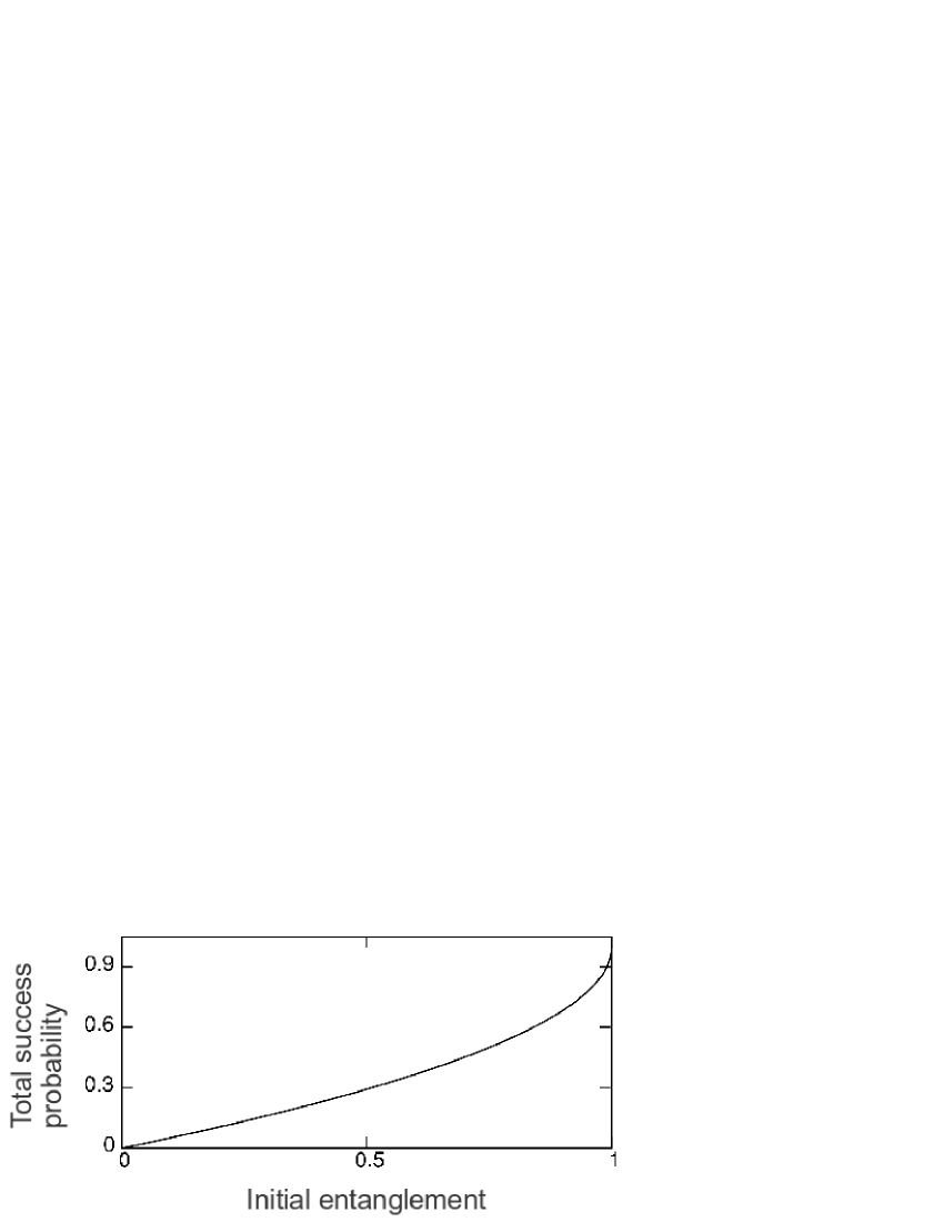
Figure 3: Total success probability versus initial entanglement. The horizontal axis represents the linear entropy $S(|\psi\rangle)$ of the state $|\psi\rangle$. The total success probability is defined as the asymptotic value of the sum of the net probability, as shown in figure 2(c).

Let us now characterize better the present approach. The $n$th measurement is used when the previous weak measurement apparatus shows the outcome $\hat{M}_{-}^{\dagger}\hat{M}_{-}$. Thus, we may define the net probability to find a maximally entangled state at the $n$th step as

$$P_{n}^{{\rm net}}=P_{n}\prod_{k=1}^{n-1}(1-P_{k}),$$ (11)

if $n\geq 2$ and $P_{1}^{{\rm net}}=P_{1}$. We find that $P_{n-1}^{{\rm net}}>P_{n}^{{\rm net}}$. The sum of the net probabilities is a characteristic quantity of this scheme. We define $P_{n}^{{\rm s}}$ as

$$P_{n}^{{\rm s}}=\sum_{m=1}^{n}P_{m}^{{\rm net}}.$$ (12)

This quantity obeys the recurrence relation $P^{\rm s}_{n}=P^{\rm s}_{n-1}+(1-P_{n})P^{\rm s}_{n-1}$ if $n\geq 2$ and $P^{\rm s}_{1}=P_{1}$. Figure 2(c) shows that $P^{\rm s}_{n}$ approaches a specific value for large $n$. We confirm that this asymptotic value is $2\alpha^{2}$ by numerically calculating $P^{\rm s}_{n}$ for the various initial states. We call this asymptotic value the total success probability of the approach. Figure 3 shows that the total success probability is large when $\alpha$ is close of $\frac{1}{2}$ [or $S(\psi)$ is close to its maximum value]. Here, we show an alternative evaluation of the total success probability. We consider an asymptotic map corresponding to the entire protocol. First, we focus on the fact that the entire protocol in the limit $n\to\infty$ can be regarded as a CPTP map

$$|\psi\rangle\langle\psi|\mapsto\rho_{\ast}=P_{\ast}|\psi_{\rm MES}\rangle\langle\psi_{\rm MES}|+(1-P_{\ast})|\chi\rangle\langle\chi|,$$ (13)

where $|\psi_{\rm MES}\rangle=(|0\rangle|\phi_{0}\rangle+|1\rangle|\phi_{1}\rangle)/\sqrt{2}$, and $|\chi\rangle=|1\rangle|\phi_{1}\rangle$. The positive coefficient $P_{\ast}$ corresponds to the total success probability. This map must be a composite map of the weak measurements (4). Therefore, we may write $\rho_{\ast}$ as

$$\rho_{\ast}=\sum_{\sigma=+,-}(\hat{M}_{\ast,\sigma}\otimes\hat{I}_{d})|\psi\rangle\langle\psi|(\hat{M}_{\ast,\sigma}\otimes\hat{I}_{d})^{\dagger},$$ (14)

$$\hat{M}_{\ast,\pm}=\sqrt{\frac{1\pm\delta_{0}}{2}}|0\rangle\langle 0|+\sqrt{\frac{1\pm\delta_{1}}{2}}|1\rangle\langle 1|,$$ (15)

with $|\delta_{0}|,\,|\delta_{1}|\leq 1$. The measurement operators $\hat{M}_{\ast,\pm}$ correspond to generalized weak (partial) measurements [26, 27]. We find that (14) represents a convex combination between $|\psi_{{\rm MES}}\rangle\langle\psi_{{\rm MES}}|$ and $|\chi\rangle\langle\chi|$ if

$$(\hat{M}_{\ast,+}\otimes\hat{I}_{d})|\psi\rangle\propto|\psi_{{\rm MES}}\rangle,\quad(\hat{M}_{\ast,-}\otimes\hat{I}_{d})|\psi\rangle\propto|\chi\rangle.$$ (16)

Let us put $\delta_{0}=1$ and $\beta\sqrt{(1+\delta_{1})/2}=\alpha$. Then, we find that $(\hat{M}_{\ast,+}\otimes\hat{I}_{d})|\psi\rangle=\sqrt{2}\alpha|\psi_{\rm MES}\rangle$. Thus, we show that

$$P_{\ast}=2\alpha^{2}.$$ (17)

In other words, we decomposed the map $(\ref{eq:asymp_map})$ with (4), as pointed out in [30]. The measurement operators $\hat{M}_{\ast,+}$ and $\hat{M}_{\ast,-}$ for $\delta_{0}=1$ was experimentally demonstrated as a partial-collapse measurement in [16, 20, 28]. We remark that the asymptotic map can be regarded as a single-shot partial measurement and is equal to the Procrustean method in [19]. Actually, the total success probability $P_{\ast}$ is the same as the yield of maximally-entangled states in  [19].

Let us compare the present entanglement amplification protocol to the Procrustean method in [19] from the viewpoint of physical implementation. The present approach requires the implementation of weak measurements that are symmetric or balanced with respect to the measurement strength, as seen in (4). Such symmetric weak measurements can be implemented in various physical systems including linear optical and solid-state qubits, as shown, e.g., in [29]. In contrast to the symmetric measurements, the Procrustean method uses non-symmetric ones. Namely, one uses (15) with $\delta_{0}=1$ and $\delta_{1}\neq-1$. Although the non-symmetric partial measurements are naturally realized in, e.g., Josephson phase qubits [28], they are not always available in a general physical system. Thus, when one has a physical system in which the implementation of the type of non-symmetric partial measurements that are used in [19] is difficult, one can use the present approach as an alternative method for entanglement distillation of a single copy of a pure state.

4 Mixed states

We now extend our approach to a mixed initial state. Hereafter, we consider a two-qubit system (i.e., $d=2$). The study of a mixed initial state is motivated by experimental considerations, as well as theoretical interest. One may desire to amplify entanglement of a quantum state in the presence of decoherence, for example. We remark that one never distills a maximally-entangled state from a single copy of a mixed state with local purification protocols, as shown by Linden et al. [31] and Kent [32]. Hence, our goal in this section is to seek a protocol of increasing the entanglement of an output state compared to a mixed initial state, not purifying a maximally-entangled state. This section mainly focuses on a single-shot measurement protocol, not a repeated application of weak measurements.

The initial pure state (1) is replaced with the mixed state

$$\rho=\lambda\rho_{\rm s}+(1-\lambda)|\psi\rangle\langle\psi|,$$ (18)

where $|\psi\rangle=\alpha|00\rangle+\beta|11\rangle$ and $0\leq\lambda\leq 1$. This is a convex combination between a separable state $\rho_{\rm s}$ and a partially-entangled pure state $|\psi\rangle$. The coefficients $\alpha$ and $\beta$ are real and positive numbers in the same way as (1). The weight of the separable part is quantified by $\lambda$. We note that an arbitrary density matrix on $\mathbb{C}^{2}\otimes\mathbb{C}^{2}$ can be written by the form (18), and this decomposition is uniquely determined [35]. We use the concurrence [33, 34] to evaluate the entanglement of a mixed state. Hereafter, the concurrence of $\rho$ is written as $C(\rho)$. We also use another quantity to estimate entanglement in addition to the concurrence. When a mixed state is given as the form (18), its entanglement can be characterized by its pure-state part $(1-\lambda)|\psi\rangle\langle\psi|$ [35]. Thus, an intuitive “measure” of entanglement is defined as $E(\rho)=(1-\lambda)S(\psi)$, with the linear entropy (2). Using both $C(\rho)$ and $E(\rho)$, we examine the entanglement amplification protocol for (18). Hereafter, we assume that $\lambda\neq 0$ and $\beta>\alpha$.

We use the same local two-outcome weak measurement in the case of a pure initial state. As seen in section 3, performing a single measurement whose measurement operator is given by (4), we obtain $\rho_{\rm out}=R_{+}\rho_{+}+R_{-}\rho_{-}$, with $R_{\pm}=\lambda w_{{\rm s},\pm}+(1-\lambda)p_{\pm}$, $\rho_{\pm}=(\hat{M}_{\pm}\otimes\hat{I}_{2})\rho(\hat{M}_{\pm}^{\dagger}\otimes\hat{I}_{2})/R_{\pm}$, and $w_{{\rm s},\pm}=\mbox{tr}\,[(\hat{M}_{\pm}^{\dagger}\hat{M}_{\pm}\otimes\hat{I}_{2})\rho_{\rm s}]$. Our aim is to increase the entanglement of $\rho_{+}$, compared with $\rho$. This density matrix has the same form as (18),

$$\rho_{+}=\lambda_{+}\frac{(\hat{M}_{+}\otimes\hat{I}_{2})\rho_{\rm s}(\hat{M}_{+}^{\dagger}\otimes\hat{I}_{2})}{w_{{\rm s},+}}+(1-\lambda_{+})|\psi_{+}\rangle\langle\psi_{+}|,$$ (19)

with

$$\lambda_{+}=\frac{w_{{\rm s},+}}{R_{+}}\lambda.$$ (20)

We examine $E(\rho)$ and $E(\rho_{+})$ to obtain a simple criterion for the entanglement amplification. Since $\rho_{\rm s}$ is a separable density matrix and the weak measurement is local, the first term in (19) is the separable part of $\rho_{+}$. Therefore, $E(\rho_{+})=(1-\lambda_{+})S(\psi_{+})$. As shown in section 3, $|\psi_{+}\rangle$ is a maximally-entangled state when the measurement strength satisfies (6). It means that $S(\psi_{+})>S(\psi)$. To ensure $E(\psi_{+})\geq E(\psi)$, we require $\lambda_{+}\leq\lambda$. This relation leads to

$$A_{{\rm s},z}\leq-\sqrt{1-S(\psi)}=\alpha^{2}-\beta^{2},$$ (21)

where we have used (6). We have defined $A_{{\rm s},z}$ as $A_{{\rm s},z}=\mbox{tr}\,[(\sigma_{z}\otimes\hat{I}_{2})\rho_{\rm s}]$, where $\sigma_{z}=|0\rangle\langle 0|-|1\rangle\langle 1|$. Therefore, we expect that the method for a pure initial state works even for a mixed initial state if this inequality is satisfied. We will check this simple criterion for specific examples using calculations of the concurrence. Then, our numerical calculations of the concurrence will show that (21) is the sufficient condition for $C(\rho_{+})\geq C(\rho)$.

4.1 Example 1: Pure dephasing

Let us consider the case when one of the subsystems (e.g., system A) travels via a noisy channel after the preparation of $|\psi\rangle$, for example. Assuming that the system undergoes pure dephasing, the corresponding CPTP map is written as $\rho\mapsto(1-u)\rho+u(\sigma_{z}\otimes\hat{I}_{2})\rho(\sigma_{z}\otimes\hat{I}_{2})$, with $0\leq u\leq 1/2$. Thus, the initial mixed state becomes

$$\rho^{({\rm pd})}=\alpha^{2}|00\rangle\langle 00|+\mu|00\rangle\langle 11|+\mu|11\rangle\langle 00|+\beta^{2}|11\rangle\langle 11|,$$ (22)

with $\mu=\alpha\beta(1-2u)$. We can rewrite (22) as $\rho^{({\rm pd})}=[1-(\mu/\alpha\beta)](\alpha^{2}|00\rangle\langle 00|+\beta^{2}|11\rangle\langle 11|)+(\mu/\alpha\beta)|\psi\rangle\langle\psi|$. Non-classical features of this sort of density matrices are characterized well by the off-diagonal element $\mu$ [36]. In fact, the concurrence is $C(\rho^{({\rm pd})})=2\mu$. Let us check the inequality (21). Since $A_{{\rm s},z}=\alpha^{2}-\beta^{2}$ and $\sqrt{1-S(\psi)}=\beta^{2}-\alpha^{2}$, the left hand side of (21) is zero and the inequality is satisfied. Thus, we expect that the approach for a pure initial state leads to an amplification of the entanglement of $\rho^{({\rm pd})}$. We calculate the concurrence to confirm that this prediction is correct. The concurrence of $\rho^{({\rm pd})}_{+}\propto(\hat{M}_{+}\otimes\hat{I}_{2})\rho^{({\rm pd})}(\hat{M}_{+}^{\dagger}\otimes\hat{I}_{2})$ is

$$C(\rho_{{\rm pd},+})=\frac{\mu}{\alpha\beta}>2\mu=C(\rho^{({\rm pd})}).$$ (23)

Therefore, entanglement amplification is achieved. Furthermore, we can find that the repeated application still works. The input density matrix for the $n$th measurement apparatus is the state corresponding to the outcome $\hat{M}_{-}^{\dagger}(\epsilon_{n-1})\hat{M}_{-}(\epsilon_{n-1})$. We denote this state as $\rho_{n}$. We note that $\rho_{1}=\rho^{({\rm pd})}$. When we obtain the outcome $\hat{M}_{+}^{\dagger}(\epsilon_{n})\hat{M}_{+}(\epsilon_{n})$, the measurement is considered to be successful. We write the resultant state as $\rho^{({\rm s})}_{n}$. The measurement strength obeys the recurrence relation (9) with $\epsilon_{1}=\sqrt{1-S(\psi)}$. The application to $\rho$ is straightforward because $\rho_{n}$ and $\rho^{({\rm s})}_{n}$ have the same form as $\rho$ (i.e., only the coefficients change). We can show that $C(\rho^{({\rm s})}_{n})>C(\rho_{n})$ and $C(\rho_{n})<C(\rho_{n-1})$. Eventually, we find that $C(\rho^{({\rm s})}_{n})=C(\rho^{({\rm s})}_{n-1})$. Therefore, at every value for the outcome $\hat{M}_{+}^{\dagger}\hat{M}_{+}$, we obtain a mixed state with the concurrence $C(\rho^{({\rm s})}_{1})=\mu/\alpha\beta$. Remarkably, we find that $\mu/\alpha\beta>C(\rho^{({\rm pd})})$ because $2\alpha\beta<1$. The resultant entanglement is bounded by $\mu/\alpha\beta$, which is regarded as a measure of the purity of $\rho^{({\rm pd})}$.

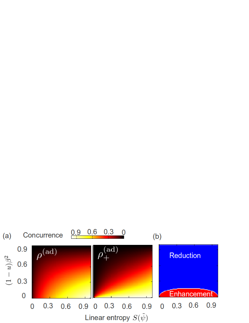
Figure 4: (Color online) Characteristics of the entanglement amplification method for the mixed state associated with amplitude damping, (24). The horizontal axis is the linear entropy of the reduced density matrix of the pure-state part, $S(\tilde{\psi})$. The vertical axis is the weight of the separable part, $(1-u)\beta^{2}$. (a) Concurrence of the input state $\rho^{({\rm ad})}$ (left panel) and the output state $\rho^{({\rm ad})}_{+}$ (right panel). Using (6), the measurement strength is given by $\sqrt{1-S(\tilde{\psi})}$. (b) Profile of ${\rm sgn}[C(\rho^{({\rm ad})}_{+})-C(\rho^{({\rm ad})})]$. When this quantity is positive, the entanglement amplification is achieved (red-colored region). Otherwise, the protocol fails (blue-colored region).

4.2 Example 2: Amplitude damping

The second example is associated with amplitude-damping. If this effect occurs on system A, the corresponding CPTP map is written as $\rho\mapsto\sum_{\ell=1,2}(\hat{E}_{\ell}\otimes\hat{I}_{2})\rho(\hat{E}_{\ell}^{\dagger}\otimes\hat{I}_{2})$, with $\hat{E}_{1}=|0\rangle\langle 0|+\sqrt{u}|1\rangle\langle 1|$, $\hat{E}_{2}=\sqrt{1-u}|0\rangle\langle 1|$, and $0\leq u\leq 1$. Thus, the mixed state becomes

$$\rho^{({\rm ad})}=(1-u)\beta^{2}|01\rangle\langle 01|+[1-(1-u)\beta^{2}]|\tilde{\psi}\rangle\langle\tilde{\psi}|,$$ (24)

with $|\tilde{\psi}\rangle=(\alpha|00\rangle+\sqrt{u}\beta|11\rangle)/\sqrt{1-(1-u)\beta^{2}}$. Assuming that $\sqrt{u}\beta>\alpha$, we check the inequality (21). Since $\sqrt{1-S(\tilde{\psi})}=(u\beta^{2}-\alpha^{2})/(u\beta^{2}+\alpha^{2})>0$ and $A_{{\rm s},z}=1$, (21) is not satisfied. Thus, we expect that the method for a pure initial state does not work. A numerical calculation of the concurrence gives more quantitative characterization of our protocol, as seen in figure 4. Varying the weight of the separable part $(1-u)\beta^{2}$ and the linear entropy of the reduced density matrix of the pure-state part $S(\tilde{\psi})$, the concurrences of $\rho^{({\rm ad})}$ [left panel of figure 4(a)] and $\rho^{({\rm ad})}_{+}\propto(\hat{M}_{+}\otimes\hat{I}_{2})\rho^{({\rm ad})}(\hat{M}_{+}^{\dagger}\otimes\hat{I}_{2})$ [right panel of figure 4(a)] are calculated. Furthermore, the sign of their difference ( ${\rm sgn}[C(\rho^{({\rm ad})}_{+})-C(\rho^{({\rm ad})})]$ ) is evaluated, as seen in figure 4(b). Figure 4(b) shows that the method for a pure state leads to the reduction of the entanglement in wide parameter region. Nevertheless, when the purity of $\rho^{({\rm ad})}$ is large, the entanglement is amplified.

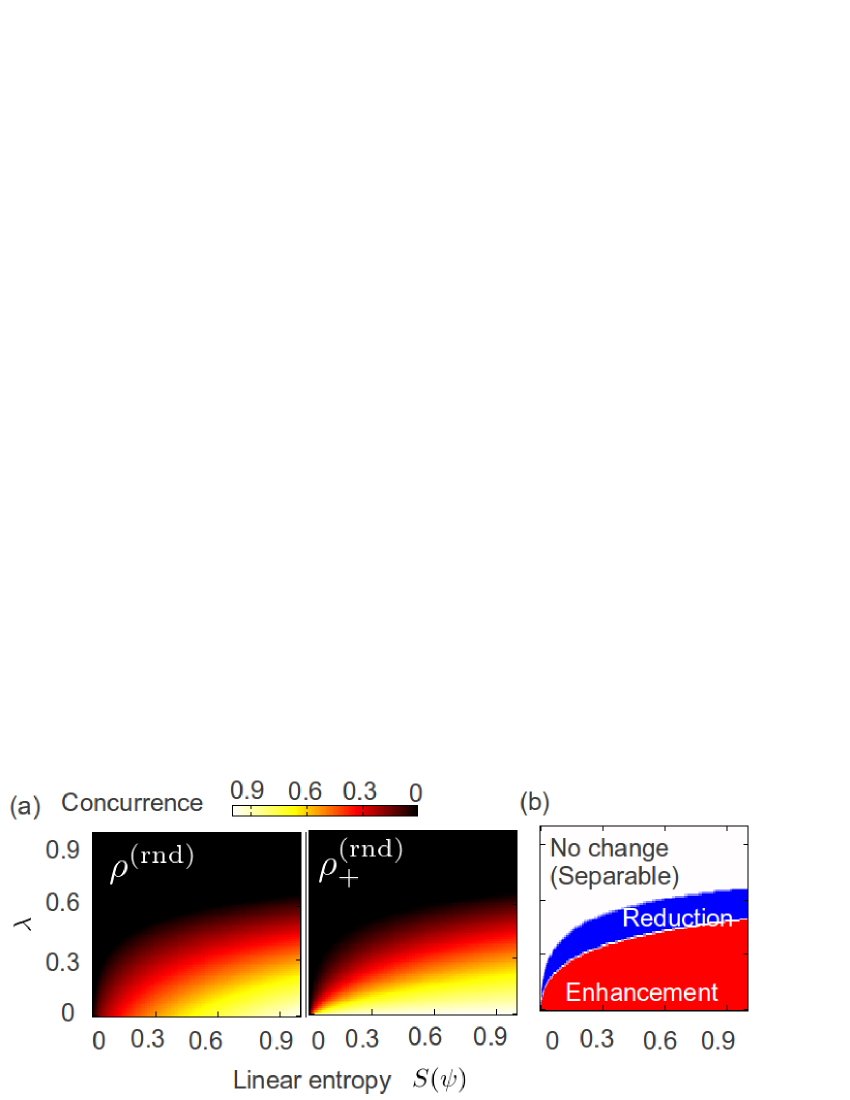
Figure 5: (Color online) Characteristics of the entanglement amplification method for the initial state (25). The horizontal axis is the linear entropy of the reduced density matrix of a pure-state part, $S(\psi)$. The vertical axis is the weight of the separable part, $\lambda$. (a) Concurrence of the input state $\rho^{({\rm rnd})}$ (left panel) and the output state $\rho^{({\rm rnd})}_{+}$ (right panel). Using (6), the measurement strength is given by $\sqrt{1-S(\psi)}$. (b) Profile of ${\rm sgn}[C(\rho^{({\rm rnd})}_{+})-C(\rho^{({\rm rnd})})]$. When this quantity is positive, the entanglement amplification is achieved (red-colored region). Otherwise, the protocol fails (blue-colored region). In the white-colored region, the concurrence does not change because the initial mixed state (25) is separable.

4.3 Example 3: Maximally-mixed state

The parameter region in which the entanglement amplification for mixed states works depends on the value of $A_{{\rm s},z}$. Let us examine the case when the separable state in (18) is the maximally-mixed state, for example. The initial mixed state becomes

$$\rho^{({\rm rnd})}=\lambda\frac{1}{4}\hat{I}_{2}\otimes\hat{I}_{2}+(1-\lambda)|\psi\rangle\langle\psi|.$$ (25)

We find that $A_{{\rm s},z}=0$. Therefore, the inequality (21) is not satisfied except for $S(\psi)=1$. In order to evaluate quantitative behaviors of the protocol, let us examine the concurrence. Figure 5(a) shows the concurrences of $\rho^{({\rm rnd})}$ (left panel) and $\rho^{({\rm rnd})}_{+}\propto(\hat{M}_{+}\otimes\hat{I}_{2})\rho_{{\rm rd}}(\hat{M}_{+}^{\dagger}\otimes\hat{I}_{2})$ (right panel). The sign of their difference (${\rm sgn}[C(\rho^{({\rm rnd})}_{+})-C(\rho^{({\rm rnd})})]$ ) is shown in figure 5(b). Again, we find that the method for a pure state fails in wide parameter region. However, compared with figure 4(b), the entanglement amplification is achieved in much wider region. Thus, smaller values of $A_{{\rm s},z}$ lead to higher success of the protocol for various parameters. We also find that from (21) negative values of $A_{{\rm s},z}$ are preferable for the entanglement amplification.

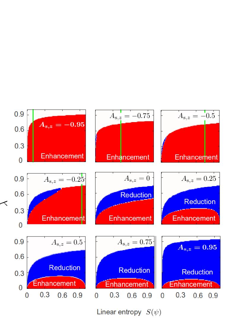
Figure 6: (Color online) Profiles of concurrence differences between the output and the initial states, varying $A_{{\rm s},z}$. Each point is a mean value over $10000$ separable states. The horizontal axis is the linear entropy of the reduced density matrix of the pure-state part. The vertical axis is the weight of the separable part. See (18). When the differences are positive (red-colored regions), the entanglement amplification is achieved. Otherwise, the protocol fails (blue-colored regions). In the white-colored regions, the concurrence does not change because the mixed initial state is separable. In the right regions of the the vertical (green) lines, the inequality (21) is satisfied.

4.4 Systematic examinations

For a more systematic analysis for mixed initial states, we randomly generate separable density matrices. Thus, we examine entanglement amplification for various density matrices given by (18), with fixed $|\psi\rangle$. A separable state on $\mathbb{C}^{2}\otimes\mathbb{C}^{2}$ is parametrized by $15$ real parameters. Using the Pauli matrices, we can express it as

$$\rho_{\rm s}=\frac{1}{4}\left(\hat{I}_{2}\otimes\hat{I}_{2}+\sum_{i}A_{{\rm s},i}\sigma_{i}\otimes\hat{I}_{2}+\sum_{j}B_{{\rm s},j}\hat{I}_{2}\otimes\sigma_{j}+\sum_{i,j}C_{{\rm s},ij}\sigma_{i}\otimes\sigma_{j}\right),$$ (26)

with $i,j=x,y,z$ and $A_{{\rm s},i},B_{{\rm s},j},C_{{\rm s},ij}\in\mathbb{R}$. The positivity and the separability of (26) give constraints with respect to the real parameters $A_{{\rm s},i}$, $B_{{\rm s},j}$, and $C_{{\rm s},ij}\in\mathbb{R}$. The former is straightforwardly checked using Newton’s formula (see, e.g., [37]). The latter is checked by the positive partial transpose criterion [38, 39]. We calculate the mean values of the concurrences of $\rho$ and $\rho_{+}$ with respect to randomly-generated separable states. Then, we evaluate ${\rm sgn}[\overline{C}(\rho_{+})-\overline{C}(\rho)]$, where $\overline{C}$ represents the mean value of the concurrence. To examine the $A_{{\rm s},z}$ dependence of the protocol, we randomly generate $\rho_{{\rm s}}$ fixing $A_{\rm s}$ as a specific value. We generate $10000$ samples for each value of $A_{{\rm s},z}$ using the Mersenne Twister method [40]. Figure 6 shows ${\rm sgn}[\overline{C}(\rho_{+})-\overline{C}(\rho)]$, varying $A_{{\rm s},z}$. When this difference is positive (red-colored regions), the entanglement amplification is achieved. We note that in the white-colored region the entanglement is not changed because the mixed initial states are separable. The vertical (green) lines (for $A_{{\rm s},z}=-0.95,\,-0.75,\,-0.55,\,-0.35$) corresponds to the equality of (21), $S(\psi)=1-(A_{{\rm s},z})^{2}$. In the right regions of the lines, the inequality (21) is satisfied. Thus, figure 6 shows that (21) is the sufficient condition for $C(\rho_{+})\geq C(\rho)$. Furthermore, when $A_{{\rm s},z}$ is a large negative value, the entanglement is enhanced in wide parameter region.

Summarizing the above arguments, the inequality (21) is the sufficient condition for the entanglement amplification. In addition, the method for a pure intial state can still lead to entanglement amplification even for a mixed initial state if the separable part of the mixed state fulfills $A_{{\rm s},z}<0$. The reason why negative values of $A_{{\rm s},z}$ are preferable for the entanglement amplification is understood by considering the role of the measurement operator $\hat{M}_{+}$ in the present protocol. When the measurement strength fulfills (6), $\hat{M}_{+}$ reduces components with respect to $|1\rangle$ of an input state $\rho$ (e.g., $\langle 11|\rho|11\rangle$). A large negative value of $A_{{\rm s},z}$ implies that $\mbox{tr}\,[(|1\rangle\langle 1|\otimes\hat{I}_{2})\rho_{\rm s}]$ is a predominant component of the separable part of the input state. Therefore, the measurement operator $\hat{M}_{+}$ considerably decreases the weight of the separable part in the input density matrix. We remark that positive values of $A_{{{\rm s},z}}$ are preferable for the entanglement amplification when $\alpha>\beta$ and the measurement strength satisfies $\epsilon=\alpha^{2}-\beta^{2}(>0)$.

5 Implementing the protocol with general measurements

We mention that no specific type of weak measurements is essential for this approach. We can use a generalized two-outcome measurement,

$$\hat{M}_{1}=\sqrt{p}|0\rangle\langle 0|+\sqrt{q}|1\rangle\langle 1|,$$ (27)

$$\hat{M}_{2}=\sqrt{1-p}|0\rangle\langle 0|+\sqrt{1-q}|1\rangle\langle 1|,$$ (28)

with $0\leq p\leq 1$ and $0\leq q\leq 1$. We note that in the Procrustean method one of the two parameters is fixed as $1$. The two real parameters $p$ and $q$ may be determined by the requirements $|\psi\rangle=|\psi_{\rm MSE}\rangle$ and $\lambda_{+}\leq\lambda$, given as, respectively,

$$p\alpha^{2}=q\beta^{2},$$ (29)

$$(p-q)(\sqrt{1-S(\psi)}+A_{{\rm s},z})\leq 0.$$ (30)

For pure initial states, the latter condition is not necessary. Adjusting the two real parameters depending on the initial partially-entangled state and the separable part, we may achieve entanglement amplification with some probability. Alternatively, we may use a continuous weak measurement. Continuously monitoring system A with very weak measurement strength, the entanglement of formation of the total system may fluctuate and take its maximal value $1$ at some point in time. We note that both of them have the same efficiency as the Procrustean method.

6 Summary

We have proposed a local probabilistic protocol to make a maximally-entangled state from a partially-entangled pure state by applying elementary two-outcome weak measurements. The present approach requires only the implementation of local measurements and the information of the initial entanglement. The probability to find the maximally-entangled state at each step decreases to zero with increasing measurement number. In addition, we found that the present approach corresponds to a decomposition of a two-outcome POVM which generates maximally-entangled or separable states as the measurement results. The success probability of the map corresponding to this POVM is high if the initial entanglement is large. The case for a mixed initial state was also examined. We found that the method for a pure state still leads to entanglement amplification, but not purifying a maximally-entangled state, if the separable part satisfies a certain condition. Several future issues will contribute to the development of weak measurement-based quantum control and the illustration of interesting and useful properties of POVM’s.

An interesting application example of this method is a quantum network system in which system A is a mediator (e.g., photon) and system B is a quantum memory. In this case, it is not easy to perform controlled operations between the two systems after their initial preparation. A local-operation-based approach will be effective for such a situation.

References

References

- [1] Davies E B 1976 Quantum Theory of Open Systems (Academic Press, London)
- [2] Kraus K 1983 1983 States, Effects and Operations: Fundamental Notations of Quantum Theory (Springer, Berlin)
- [3] Peres A 1993 Quantum Theory: Concepts and Methods (Kluwer Academic Publishers, Dordrecht)
- [4] D’Espagnat B 1999 Conceptual Foundations of Quantum Mechanics Second edition (Westview Press, Colorado)
- [5] Misra B and Sudarshan E C G 1977 J. Math. Phys. 18 756
- [6] Nakazato H, Namiki M and Pascazio S 1996 Int. J. Mod. Phys. B 10 247
- [7] Raussendorf R, Browne D E and Briegel H J 2003 Phys. Rev. A 68 022312
- [8] Facchi P, Lidar D A and Pascazio S 2004 Phys. Rev. A 69 032314
- [9] Sun Q, Al-Amri M, Davidovich L and Zubairy M S 2010 Phys. Rev. A 82 052323
- [10] Korotkov A N and Keane K 2010 Phys. Rev. A 81 040103(R)
- [11] Paz-Silva G A, Rezakhani A T, Dominy J M and Lidar D A 2011 Zeno effect for quantum computation and control arXiv:1104.5507
- [12] Yuasa K, Burgarth D, Giovannetti V and Nakazato H 2009 New J. Phys. 11 123027
- [13] Braczyk A M, Mendonça P E M F, Gilchrist A, Doherty A C and Bartlett S D 2007 Phys. Rev. A 75 012329
- [14] Ashhab S and Nori F 2010 Phys. Rev. A 82 062103; Wiseman H M 2011 Nature 470 178
- [15] Koashi M and Ueda M 1999 Phys. Rev. Lett. 82 2598
- [16] Kim Y S, Cho Y W, Ra Y S and Kim Y H 2009 Opt. Express 17 11978
- [17] Iinuma M, Suzuki Y, Taguchi G, Kadoya Y and Hofmann F 2011 New J. Phys. 13 033041
- [18] Kofman A G, Ashhab S and Nori F 2012 Phys. Rep. 520 43
- [19] Bennett C H, Bernstein H J, Popescu S and Schumacher B 1996 Phys. Rev. A 53 2046
- [20] Kwiat P G, Barraza-Lopez S, Stefanov A and Gisin N 2001 Nature 409 1014
- [21] Bru D and Leuchs G (eds) 2007 Lectures on Quantum Information edited by D. Bru and G. Leuchs (Wiley-VCH, Weinheim, 2007).
- [22] Maruyama K and Nori F 2008 Phys. Rev. A 78 022312
- [23] Yamamoto T, Koashi M, Özdemir S K and Imoto N 2003 Nature 421 343
- [24] Pan J W, Gasparoni S, Ursin, Weihs G and Zeilinger A 2003 Nature 423 417
- [25] Nagali E, Felicetti S, de Assis P L, D’Ambrosio V, Filip R and Sciarrino F 2011 Sci. Rep. 2 443
- [26] Paraoanu G S 2011 Europhys. Lett. 93 64002
- [27] Paraoanu G S 2011 Found. Phys. 41 1214
- [28] Katz N, Neeley M, Ansmann M, Bialczak R C, Hofheinz M, Lucero E, O’Connell A, Wang H, Cleland A N, Martinis J M and Korotkov A N 2008 Phys. Rev. Lett. 101 200401
- [29] Ota Y, Ashhab S and Nori F 2012 Phys. Rev. A 85 043808
- [30] Oreshkov O and Brun T A 2005 Phys. Rev. Lett. 95 110409
- [31] Linden N, Massar S and Popescu S 1998 Phys. Rev. Lett. 81 3279
- [32] Kent A 1998 Phys. Rev. Lett. 81 2839
- [33] Wootters W K 1998 it Phys. Rev. Lett. 80 2245
- [34] Audenaert K, Verstraete F and De Moor B 2001 Phys. Rev. A 64 052304
- [35] Lewenstein M and Sanpera A 1998 Phys. Rev. Lett. 80 2261
- [36] Ashhab S, Maruyama K and Nori F 2007 Phys. Rev. A 76 052113
- [37] Kimura G 2003 Phys. Lett. A 314 229
- [38] Peres A 1996 Phys. Rev. Lett. 77 1413 (1996)
- [39] Horodecki M, Horodecki P and Horodecki R 1996 Phys. Lett. A 223 1
- [40] Matsumoto M and Nishimura T 1998 ACM Trans. on Modeling and Computer Simulation 8 3