Difference of energy density of states in the Wang-Landau algorithm

Abstract

Paying attention to the difference of density of states, $\Delta\ln g(E)\equiv\ln g(E+\Delta E)-\ln g(E)$, we study the convergence of the Wang-Landau method. We show that this quantity is a good estimator to discuss the errors of convergence, and refer to the $1/t$ algorithm. We also examine the behavior of the 1st-order transition with this difference of density of states in connection with Maxwell’s equal area rule. A general procedure to judge the order of transition is given.

The Monte Carlo simulation has become a standard method to study many-body problems in physics. However, we sometimes suffer from the problem of slow dynamics in the original Metropolis algorithm metro53 . One attempt to conquer the problem of slow dynamics is the extended ensemble method; one uses an ensemble different from the ordinary canonical ensemble with a fixed temperature. The multicanonical method berg91 ; berg92 , the parallel tempering, or the exchange Monte Carlo method hukushima ; marinari and the Wang-Landau (WL) algorithm wl01 are examples. The WL method is an efficient algorithm to calculate the energy density of states (DOS), $g(E)$, with high accuracy, and was successfully applied to many problems yamaguchi01 ; okabe06 . The refinement and convergence of the WL method were argued zhou05 ; lee06 , but the convergence property is still a topic of discussions belardinelli07b . The search for optimal modification factor was discussed zhou08 , and in connection with the WL method, the $1/t$ algorithm belardinelli07 ; belardinelli08 was proposed. Moreover, tomographic entropic sampling scheme has been proposed as an algorithm to calculate DOS dickman .

In this paper, we investigate the convergence properties of the WL method, paying special attention to the difference of DOS. We argue its relevance to the 1st-order transition. We provide a general strategy to judge the order of transition.

Let us briefly review the WL algorithm. A random walk in energy space is performed with a probability proportional to the reciprocal of the DOS, $1/g(E)$, which results in a flat histogram of energy distribution. Actually, we make a move based on the transition probability from energy level $E_{1}$ to $E_{2}$

$$p(E_{1}\to E_{2})=\min\Big{[}1,\frac{g(E_{1})}{g(E_{2})}\Big{]}.$$ (1)

Since the exact form of $g(E)$ is not known a priori, we determine $g(E)$ iteratively. Introducing the modification factor $f_{i}$, $g(E)$ is modified by

$$\ln g(E)\to\ln g(E)+\ln f_{i}$$ (2)

every time the state is visited. At the same time the energy histogram $h(E)$ is updated as

$$h(E)\to h(E)+1.$$ (3)

The modification factor $f_{i}$ is gradually reduced to unity by checking the ‘flatness’ of the energy histogram. The ’flatness’ is checked such that the histogram for all possible $E$ is not less than some value of the average histogram, say, 80%. Then, $f_{i}$ is modified as

$$\ln f_{i+1}=\frac{1}{2}\ln f_{i}$$ (4)

and the histogram $h(E)$ is reset. As an initial value of $f_{i}$, we choose $f_{0}=e$; as a final value, we choose $\ln f_{i}=2^{-26}$, that is, $f_{26}\simeq 1.000\,000\,01$, for example.

We first treat the Ising model, whose Hamiltonian is given by

$$\mathcal{H}=-J\sum_{\langle i,j\rangle}\sigma_{i}\sigma_{j}.$$ (5)

Here, $J$ is the coupling and $\sigma_{i}$ is the Ising spin ($\pm 1$) on the lattice site $i$. The summation is taken over the nearest neighbor pairs $\langle i,j\rangle$. Periodic boundary conditions are employed. Throughout this paper, we measure the energy in units of $J$ unless specified; in other words, we put $J=1$.

We calculate $\ln g(E)$ with the use of the WL method, and consider the difference of $\ln g(E)$, which is defined as

$$\Delta\ln g(E)\equiv\ln g(E+\Delta E)-\ln g(E).$$ (6)

For the Ising model, $\Delta E=4J$. The exact value of $g(E)$ for the two-dimensional (2D) Ising model is available due to Beale beale . The deviation of the calculated value of $\Delta\ln g(E)$ from the exact value of Beale beale can be used as a measure of the accuracy of the calculation.

We plot the overall behavior of $\Delta\ln g(E)$ for the 2D Ising model with system size $L$ = 32 in Fig. 1. The data for the modification step $i$ = 14, 18 and 22 are given for a single measurement. In the accuracy of this plot, little difference in $i$ is appreciable except for small and large $E$. The enlarged plot near $E=0$ is given in the inset of Fig. 1, and the data for $i$ = 14, 18 and 22 are compared to the exact value of Beale beale . We see that the calculated value of $\Delta\ln g(E)$ approaches the exact value as the modification factor $f_{i}$ approaches 1. The deviation becomes smaller as $i$ increases. The advantage of using Eq. (6) is that we can directly discuss the error of DOS without caring about the normalization of $g(E)$. Since the transition probability depends on the difference of $\ln g(E_{1})$ and $\ln g(E_{2})$, this quantity of difference is essential in the method calculating the energy DOS compared to $g(E)$ itself. We note that the quantity of difference was also used in the argument of accuracy and convergence of the WL method by Morozov and Lin morozov .

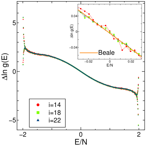
Figure 1: (Color online) Plot of $\Delta\ln g(E)$ for the 2D Ising model with $L=32$. Data for $i$ = 14, 18 and 22 are given. In the inset, the enlarged plot near $E$ = 0 is shown. The exact value due to Beale beale is also given in the inset for comparison.

To see the convergence of errors more explicitly, we consider the total sum of the squared error of $\Delta\ln g(E)-\Delta\ln g(E)_{\rm exact}$;

$$\Delta^{2}\equiv\frac{1}{N-4}\sum_{E=-2JN+8J}^{2JN-12J}\big{(}\Delta\ln g(E)-\Delta\ln g(E)_{\rm exact}\big{)}^{2}$$ (7)

For the 2D Ising model, we note that $\Delta\ln g(-2JN+8J)_{\rm exact}=-\Delta\ln g(2JN-12J)_{\rm exact}=\ln 2$.

In Fig. 2, we plot $\Delta^{2}$, Eq. (7), as a function of the modification step $i$ up to 26 for $L$ = 32. The average is taken for 10 samples. We see that $\Delta^{2}$ becomes smaller with the increase of $i$. However, the errors are saturated even though we repeat the iteration process up to $i$ = 26. Such saturation of convergence of the WL method was pointed out by Yan and de Pablo yan03 . To overcome this difficulty, a modified version of the WL algorithm in which the refinement parameter is scaled down as $1/t$ (with $t$ the Monte Carlo time) was proposed belardinelli07 ; belardinelli08 . It is interesting to compare the performance of the $1/t$ algorithm and that of the original WL method in this quantity of difference of DOS. In the $1/t$ algorithm, starting from the same condition as the original WL algorithm, the modification factor $\ln f_{i}$ is reduced as $1/t$ instead of checking the flatness condition after the condition $\ln f_{i}\leq 1/t$ is satisfied. The final value of $\ln f$ should be fixed from the outset. In Fig. 2, we also plot the data for the $1/t$ algorithm. In the case of $L=32$, the modification process is changed from the original WL scheme to the $1/t$ one around $i=$21 or 22. In the range of $1/t$ scheme the actual MCS is fixed as $2^{i}$, which is different from the case of the original WL scheme. We clearly confirm the efficiency of the $1/t$ algorithm. In the discussion of the convergence of $1/t$ algorithm, the quantity $\ln g(E)-\ln g(E_{\rm ground})$ was used belardinelli07b . The quantity given by Eq. (6) is more flexible as it can be treated even if the ground state of the system is unknown as spinglass problems.

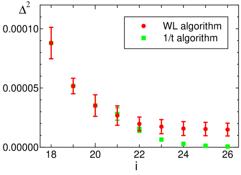
Figure 2: (Color online) Convergence of errors, $\Delta^{2}$, for the 2D Ising model with $L=32$ as a function of the modification step $i$. The convergence of the original WL algorithm is compared with that of $1/t$ algorithm. In the $1/t$ algorithm after the rule of modification is changed, the meaning of $i$ is such that MCS is $2^{i}$.

We can consider the deviation from the exact value, as in Eq. (7), for the 2D Ising model. In order to investigate the convergence behavior of the system whose exact $g(E)$ is not available, we may employ another strategy. For example, we may consider the relative error of the data for $i$ and those for $i-1$. We leave the detailed analysis to a separate publication.

Next we deal with the 2D ten-state Potts model, which is a typical model to exhibit the 1st-order transition. This model was used to show the effectiveness of the multicanonical simulation by correctly estimating the interfacial free energy berg92 , which was later proved by the explicit formula borgs . The Hamiltonian of the $q$-state Potts model is given by

$$\mathcal{H}=J\sum_{\langle i,j\rangle}\big{[}1-\delta_{S_{i},S_{j}}\big{]}.$$ (8)

Here, $S_{i}$ is the Potts spin which takes $1,\cdots,q$. We note that for $q=2$ the Potts model becomes the Ising model, although the unit of $J$ in Eq. (8) for the Potts model is twice as $J$ in Eq. (5) for the Ising model.

We plot the difference of DOS, Eq. (6), of the 2D ten-state Potts model in Fig. 3. The data for $L$ = 64 (upper) and those for $L$ = 128 (lower) are given as a function of $E/N$. We show how the data converge as $i$ increases by giving the data for $i$ = 14, 18 and 22 with a single measurement. We clearly see the convergence of errors with the increase of $i$.

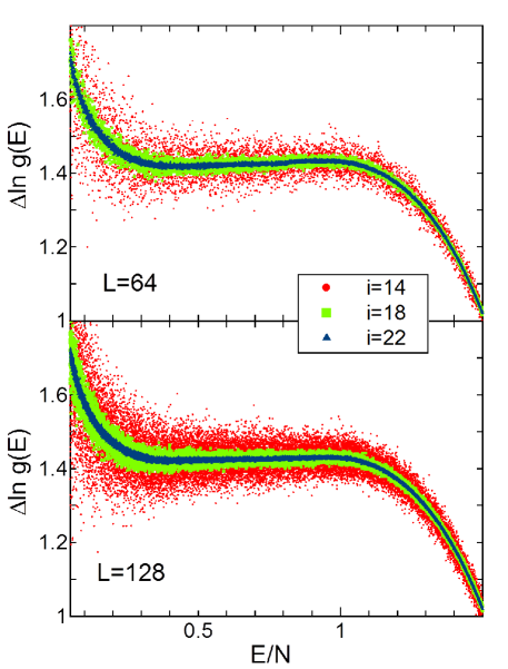
Figure 3: (Color online) Plot of $\Delta\ln g(E)$ of the 2D ten-state Potts model for $L$ = 64 (upper) and $L$ = 128 (lower) as a function of $E/N$. The data for the modification factor $f_{i}$ with $i$ = 14, 18 and 22 are given.

The systems which show the 1st-order transition have double maximum structure in the thermodynamic limit at the 1st-order transition temperature $T_{c}$ when we plot the free energy $-\beta F=\ln g(E)-\beta E$ as a function of $E$. Then, $\Delta\ln g(E)$, which is defined as Eq. (6), has an $S$-like structure with minimum and maximum. We clearly find this structure in Fig. 3. We note that the overall size dependence is small in this plot, but the detailed analysis is given later.

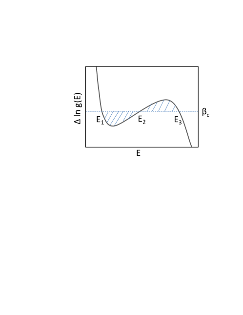
Figure 4: (Color online) Schematic illustration of Maxwell’s equal area rule.

The 1st-order transition temperature, $T_{c}=1/\beta_{c}$, can be estimated by Maxwell’s rule as in thermodynamics. A schematic illustration of Maxwell’s rule is shown in Fig. 4. The value of $\beta$, which separates the shaded region and gives the same area, becomes the 1st-order transition temperature $\beta_{c}$. This equal area rule is proved by the following. The condition that the two areas of the shaded region are equal is given by

$$-\int_{E_{1}}^{E_{2}}\frac{d\ln g(E)}{dE}\ dE+\beta(E_{2}-E_{1})$$

$$\quad=\int_{E_{2}}^{E_{3}}\frac{d\ln g(E)}{dE}\ dE-\beta(E_{3}-E_{2}),$$ (9)

which leads to the condition that the double maxima in $\ln g(E)-\beta E$ take the same value. In the thermodynamic limit, the difference $\Delta\ln g(E)$ becomes the differential $d\ln g(E)/dE$. The area of the shaded region, Eq. (9), is related to the interfacial free energy berg92 ; borgs .

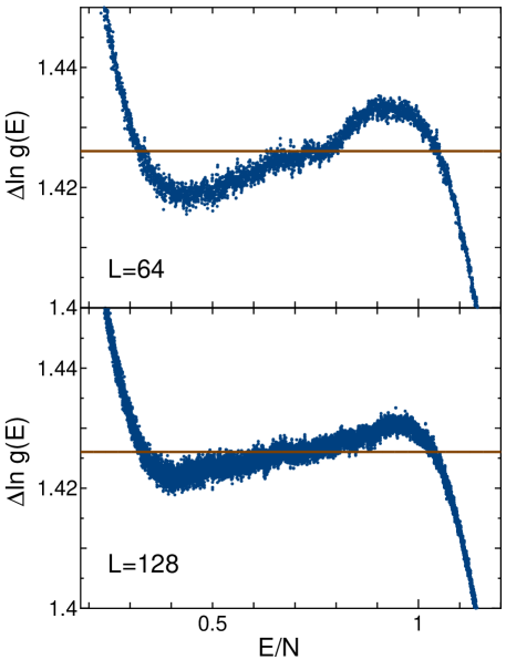
Figure 5: (Color online) Enlarged plot of $\Delta\ln g(E)$ of the 2D ten-state Potts model for $L$ = 64 (upper) and 128 (lower). The modification step $i$ is 22. The smoothed values with moving-average method are given. The 1st-order transition temperature $\beta_{c}=\ln(1+\sqrt{10})=1.42606$ in the thermodynamic limit is also shown by straight line for convenience.

To see the $S$-like structure explicitly, we make an enlarged plot along $y$-axis of $\Delta\ln g(E)$ for $L$ = 64 (upper) and 128 (lower) in Fig. 5. The modification step $i$ is 22. In this plot we use the data with the smoothing process, $(f(E-2\Delta E)+4*f(E-\Delta E)+6*f(E)+4*f(E+\Delta E)+f(E+2\Delta E))/16$ with $f(E)=\Delta\ln g(E)$, to reduce fluctuations. For the 2D ten-state Potts model, the 1st-order transition temperature is given by $\beta_{c}=\ln(1+\sqrt{10})=1.42606$. We give this value in Fig. 5 for convenience; we see that Maxwell’s rule works. We can estimate $\beta_{c}$ and the interfacial free energy from the $S$-like curve for each size. We observe the size dependence in Fig. 5; the area of the shaded region illustrated in Fig. 4 is proportional to $1/L$, which reflects on the finite size scaling of the 1st-order transition.

We may provide a general strategy to judge the order of transition for any system. We plot $\Delta\ln g(E)$ and check whether there is an $S$-like structure. If the system shows the 1st-order transition, we can locate the transition temperature by Maxwell’s rule. The behavior of the 1st-order transition can be observed in the early stage of WL iteration, that is, for small $i$. If we investigate $\ln g(E)-\beta E$ as in usual way, we have to search for $\beta$ which gives the same value for two maxima.

To summarize, we have shown that the difference of $\ln g(E)$ is a good quantity for the WL method. Less attention has been given to the quantity $\Delta\ln g(E)$ so far, although some efforts were made in the discussion of accuracy and convergence of the WL method morozov . Comparing with the exact value of the 2D Ising model, we have shown the convergence property of the WL method. That is, we have shown how errors become smaller for larger $i$, where $i$ is the step of the modification factor $f_{i}$ for the criterion of ’flatness’ condition. We have confirmed the efficiency of the $1/t$ algorithm; we have shown that the quantity $\Delta\ln g(E)$ is a good estimator for the analysis of errors of the simulation method to calculate the energy DOS.

We have also shown that $\Delta\ln g(E)$ is a good estimator for the 1st-order transition. We have investigated the 2D ten-state Potts model. The 1st-order transition is observed in the $S$-like behavior of $\Delta\ln g(E)$. We have shown that Maxwell’s equal area rule determines the 1st-order transition temperature. Although the statement is rigorously realized in the thermodynamic limit, we observe the behavior of the 1st-order transition even for small system size and for small $i$ of the modification step. We assert that we provide a general procedure to study the order of transition for any system.

The extension of this calculation to continuous spin models is straightforward zhou06 . The application to quantum Monte Carlo simulation troyer03 for checking the order of transition is highly desirable. The application to first-principle calculation of electric structure eisenbach and to protein systems gervais may be other interesting topics.s

Before closing, we mention about the calculation techniques. We have used the parallel calculation with multiple random walkers for the WL algorithm using the GPU (graphic processing unit) with CUDA (common unified device architecture). The details of the GPU-based calculation will be given elsewhere.

We thank Tasrief Surungan for valuable discussions. This work was supported by a Grant-in-Aid for Scientific Research from the Japan Society for the Promotion of Science.

References

- (1) N. Metropolis, A.W. Rosenbluth, M.N. Rosenbluth, A.H. Teller, and E. Teller, J. Chem. Phys. 21, 1087 (1953).
- (2) B. A. Berg and T. Neuhaus, Phys. Lett. B 267, 249 (1991).
- (3) B. A. Berg and T. Neuhaus, Phys. Rev. Lett. 68, 9 (1992).
- (4) K. Hukushima and K. Nemoto, J. Phys. Soc. Jpn. 65, 1604 (1996).
- (5) E. Marinari, in Advances in Computer Simulation, edited by J. Kertész and I. Kondor, (Springer-Verlag, Berlin, 1998), p. 50.
- (6) F. Wang and D.P. Landau, Phys. Rev. Lett. 86, 2050 (2001); Phys. Rev. E 64, 056101 (2001).
- (7) C. Yamaguchi and Y. Okabe, J. Phys. A: Math. Gen. 34, 8781 (2001).
- (8) Y. Okabe and H. Otsuka, J. Phys. A: Math. Gen. 39, 9093 (2006).
- (9) C. Zhou and R. N. Bhatt, Phys. Rev. E 72, 025701(R) (2005).
- (10) H. K. Lee, Y. Okabe, and D. P. Landau, Comp. Phys. Comm. 175, 36 (2006).
- (11) R. E. Belardinelli and V. D. Pereyra, J. Chem. Phys. 127, 184105 (2007).
- (12) C. Zhou and J. Su, Phys. Rev. E 78, 046705 (2008).
- (13) R. E. Belardinelli and V. D. Pereyra, Phys. Rev. E 75, 046701 (2007).
- (14) R. E. Belardinelli, S. Manzi, and V. D. Pereyra, Phys. Rev. E 78, 067701 (2008).
- (15) R. Dickman and A. G. Cunha-Netto, Phys. Rev. E 84, 026701 (2011).
- (16) P. D. Beale, Phys. Rev. Lett. 76, 78 (1996).
- (17) A. N. Morozov and S. H. Lin, Phys. Rev. E 76, 026701 (2007); J. Chem. Phys. 130, 074903 (2009).
- (18) Q. Yan and J. J. de Pablo, Phys. Rev. Lett. 90, 035701 (2003).
- (19) C. Borgs and W. Janke, J. Phys. (France) I 2, 2011 (1992).
- (20) C. Zhou, T. C. Schulthess, S. Torbrügge, and D. P. Landau, Phys. Rev. Lett. 96, 120201 (2006).
- (21) M. Troyer, S. Wessel, and F. Alet, Phys. Rev. Lett. 90, 120201 (2003).
- (22) M. Eisenbach, C.-G. Zhou, D. M. Nicholson, G. Brown, J. Larkin, and T. C. Schulthess, in: SC, Portland, Oregon, USA, November 14-20, ACM, New York (2009).
- (23) C. Gervais, T. Wüst, D. P. Landau, and Y. Xu, J. Chem. Phys. 130, 215106 (2009).