Decrypting the cyclotron effect in graphite using Kerr rotation spectroscopy

Abstract

We measure the far-infrared magneto-optical Kerr rotation and reflectivity spectra in graphite and achieve a highly accurate unified microscopic description of all data in a broad range of magnetic fields by taking rigorously the c-axis band dispersion and the trigonal warping into account. We find that the second- and the forth-order cyclotron harmonics are optically almost as strong as the fundamental resonance even at high fields. They must play, therefore, a major role in magneto-optical and magneto-plasmonic applications based on Bernal stacked graphite and multilayer graphene.

Owing to its wide spread and technological importance, graphite is one of the most studied crystalline materials. Magneto-optical spectroscopy was one of the key techniques, together with the transport and magnetization measurements, to establish the essentials of the unusual band structure of this layered semimetal. A small mass, low density and weak scattering of electrons and holes give rise to remarkably strong cyclotron resonances GaltPR56 ; SuematsuJPSJ72 ; ToyPRB77 ; DoezemaPRB79 ; NakamuraJPSJ84 ; HofmannRSI06 ; LiPRB06 ; OrlitaPRL08 ; ChuangPRB09 ; UbrigPRB11 ; TungCM11 . Surprisingly, in spite of the large number of experiments that appeared after the first report of the cyclotron effect GaltPR56 , the magneto-optical lineshapes and intensities are still not satisfactorily explained by microscopic calculations, which is in part because of the incompleteness of the existing optical data. While the measurements where circular polarization served to distinguish electrons and holes were typically done with only a few radiation wavelengths SuematsuJPSJ72 ; ToyPRB77 ; DoezemaPRB79 ; NakamuraJPSJ84 , most broadband spectroscopic experiments LiPRB06 ; OrlitaPRL08 ; ChuangPRB09 ; TungCM11 provide a highly mixed response of electrons and holes. As there exist several open questions regarding the optical intensities in graphene GusyninPRL07 ; LiNP08 ; CrasseePRB11 , a quantitative understanding of graphite as its three-dimensional counterpart is highly desirable.

In order to combine the advantages of broadband spectroscopy and a sensitivity to the charge carrier type, we measure the Kerr rotation angle $\theta_{K}(\omega)$ as a continuous function of the photon energy $\hbar\omega$, in addition to the more conventional reflectivity spectra taken on the same sample. The Kerr angle is defined as the rotation of the polarization plane upon a normal reflection of linearly polarized light from the surface of a sample, when the magnetic field $B$ is perpendicular to the surface. The reflectivity is a ratio of the intensities of the reflected and the incident beams of unpolarized radiation in the same geometry. These quantities are related to the complex reflectivity coefficients $r_{\pm}(\omega)$ for the right (+) and left (-) circular polarized light:

$$\theta_{K}=\frac{\mbox{arg}(r_{-})-\mbox{arg}(r_{+})}{2},R=\frac{|r_{-}|^{2}+|r_{+}|^{2}}{2}$$ (1)

and eventually determined, via the usual Fresnel equations, by the circular conductivities $\sigma_{\pm}(\omega)=\sigma_{xx}(\omega)\pm i\sigma_{xy}(\omega)$. While the electron and hole cyclotron resonances are indistinguishable in the reflectivity, they can be separated by the Kerr rotation. The latter has the same physical origin as the Faraday rotation CrasseeNP11 , but can be applied to opaque samples. This set of measurements can be regarded as infrared Hall spectroscopy KaplanPRL96 since it probes both the longitudinal and the Hall conductivities, $\sigma_{xx}$ and $\sigma_{xy}$, at infrared frequencies as specified in the Supplemental Material.

Figures 1a and 1b show the Kerr angle and the reflectivity of highly ordered pyrolytic graphite (HOPG) at 5 K for magnetic fields up to 7 T. The Kerr spectra are complicated and highly structured above 1 T; the structures displace in energy roughly proportionally to the field. They crossover to a simpler shape at lower fields before disappearing, as expected, at $B\rightarrow 0$. At higher fields the quantized Landau level (LL) transitions can be resolved, while at low fields different transitions merge and form a broad continuum. The reflectivity demonstrates a similar trend, except that it remains finite at zero field, and this agrees with previously taken magneto-reflectivity spectra at the corresponding photon energies and magnetic fields LiPRB06 ; TungCM11 .

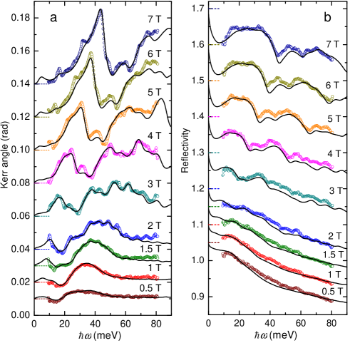
Figure 1: (color online) The Kerr angle (a) and reflectivity (b) spectra of highly ordered pyrolytic graphite measured at 5 K at various magnetic fields. The curves are offset for clarity; the dashed lines indicate 0 at panel (a) and 1 at panel (b). Circles are the experimental data, solid lines are the theoretical fits using the same set of tight-binding parameters at all fields. Note that only the Kerr angle was used to adjust the band parameters.

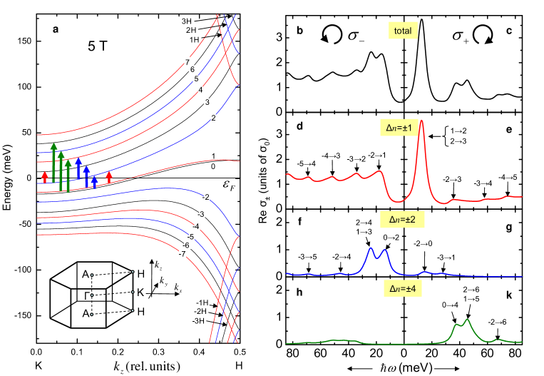
Figure 2: (color online) Panel (a): calculated low-energy Landau-level structure of graphite at 5 T. The inset shows the Brillouin zone of graphite. (b)-(k): The theoretical spectra of Re $\sigma_{+}(\omega)$ (right panels) and Re $\sigma_{-}(\omega)$ (left panels) at 5 T and 5 K. b, c: the total conductivity; (d), (e): the contribution from the fundamental transitions $\Delta n=\pm 1$; (f), (g): the contribution from the high-order transitions $\Delta n=\pm 2$; (h), (k): the same for $\Delta n=\pm 4$. The horizontal axis for the left panels is inverted for the illustration purpose, since Re $\sigma_{+}(-\omega)$ = Re $\sigma_{-}(\omega)$. Conductivities per atomic layer are shown in the units of $\sigma_{0}=e^{2}/4\hbar$. The strongest intraband transitions corresponding to the selection rules $n\rightarrow n+1$, $n\rightarrow n+2$ and $n\rightarrow n+4$ are shown in panel (a) by the red, blue and green arrows correspondingly.

The extremely small Fermi surface of graphite is elongated along the K-H line at the edge of the Brillouin zone (shown in the inset of Figure 2a), perpendicular to the graphene planes. Between K and H, the in-plane bands change continuously, the details being strongly dependent on the relative strength of the different interplane hopping parameters McClurePR57 ; SlonczewskiPR58 . However, it is often assumed in the literature that the observable spectral features originate only from the K-point, where the Fermi surface is electron-like, and from the H-point, where it is hole-like. An appealing aspect of this simplified view is that the band structure for the H-point strongly resembles the conical band dispersion of monolayer graphene, while the bands at the K point disperse parabolically similar to bilayer graphene. The LLs and therefore the cyclotron frequencies at these points are contrasted by their dependence on the perpendicular magnetic field: $\sim\sqrt{B}$ and $\sim B$ respectively ToyPRB77 ; OrlitaPRL08 .

We found that it is impossible to reproduce the measured optical curves using this two-point approximation, i.e. by considering a weighted superposition of the theoretical optical spectra of monolayer and bilayer graphene AbergelPRB07 . In contrast, taking the entire Fermi surface into account resulted in excellent fits, shown in Figures 1a and 1b as solid lines. Within this approach, the total optical conductivity is given by an integral over the K-H line NakamuraJPSJ84 ; FalkovskyPRB11

$$\sigma_{\pm}(\omega)=\int_{K}^{H}\tilde{\sigma}_{\pm}(k_{z},\omega)dk_{z}$$ (2)

where $\tilde{\sigma}_{\pm}(k_{z},\omega)$ is the partial contribution from all optically allowed transitions between LLs at a given perpendicular momentum $k_{z}$. In order to compute the LLs and optical matrix elements, we used only the conventional tight-binding parameters $\gamma_{0},...,\gamma_{5}$ and $\Delta$ of the well known Slonczewski-Weiss-McClure (SWMcC) band model McClurePR57 ; SlonczewskiPR58 and the scattering rate $\Gamma$, which we assumed, for the sake of simplicity, to be energy-, momentum- and magnetic field-independent. We took the SWMcC values from the recent magnetotransport measurements SchneiderPRL09 and fine-tuned them to fit our Kerr spectra at four field values 1, 3, 5 and 7 T simultaneously, thus covering small fields and high fields (almost up to the quantum limit LiPRB06 ; ZhuNP09 ) at the same time. Remarkably, the Kerr spectra at other fields as well as all reflectivity spectra were reproduced satisfactorily without extra fitting. The resulting parameters are fairly consistent with previous studies SchneiderPRL09 ; GruneisPRB08 . Thus in the present case the Kerr spectra alone are, in principle, sufficient to determine the electronic band parameters. The details of the calculations and the fits are given in the Supplemental Material.

One can notice that some of the LL structures, especially at low frequencies, are sharper in the experiment than in the fitting curves. This is likely due to our assumption that the scattering rate ($\Gamma\approx 2.8$ meV was found by the least-squares technique) is constant. Indeed, reducing $\Gamma$ makes the overall fit worse, but it improves the match for some spectral features.

Like it is in bilayer graphene, each LL in graphite (except for the first two) is subdivided into four sublevels, corresponding to one of the four $\pi$-bands, two electron- and two hole-like. However, in contrast to graphene, the levels in the three-dimensional graphite acquire a $k_{z}$ dispersion McClurePR57 ; NakaoJPSJ76 ; FalkovskyPRB11 , shown in Figures 2a for 5 T. We adopt the notation AbergelPRB07 ; OrlitaPRL08 ; FalkovskyPRB11 , where the main LL index $n$ starts from zero, and the minus sign is used to denote the hole sublevels. Additionally, we use the symbol H after the index to distinguish the high-energy sublevels. The LLs with $n=0$ and $n=1$ are special as they have only one and three sublevels respectively.

Although the bands and the LLs depend on all the SWMcC parameters, the symmetry of the wavefunctions and the optical selection rules are determined by the interplane next-nearest neighbor hopping $\gamma_{3}\approx 0.3$ eV. It is responsible for the so-called trigonal warping NozieresPR58 ; InoueJPSJ62 , which breaks the in-plane radial symmetry of the bands. The case of zero warping is much easier to treat analytically, since the entire Hamiltonian in a magnetic field is factorized into a series of uncoupled $4\times 4$ blocks for each LL. If $\gamma_{3}\neq 0$ then one has to diagonalize numerically an infinite matrix NakaoJPSJ76 . This case, however, is most interesting because it comprises nontrivial effects such as the magnetic breakdown in graphite NakaoJPSJ76 and Lifshitz transitions in bilayer graphene as a function of strain MuchaPRB11 . Furthermore, trigonal warping was shown to have a profound effect on the charge transport in weakly doped bilayer graphene NovoselovScience11 .

Without trigonal warping, only the transitions where the LL index $n$ changes by $\pm$1 are allowed, due to the harmonic-oscillator-like structure of the LL wavefunctions. Warping mixes LLs separated by 3 times an integer number (i.e. levels shown by the same color in Figure 2a) and makes also the high-order resonances $\Delta n=3m\pm 1$ ($m=\pm 1,\pm 2...$) optically active NozieresPR58 . These cyclotron harmonics were indeed observed GaltPR56 ; SuematsuJPSJ72 ; DoezemaPRB79 ; NakamuraJPSJ84 ; LiPRB06 and served InoueJPSJ62 ; SuematsuJPSJ72 ; DoezemaPRB79 to determine $\gamma_{3}$. However, little is known about the absolute optical strength of these transitions. The very good match between the data and the theory allows us to clarify this issue.

Figures 2b and 2c show the real parts of the total right and left-handed optical conductivities as given by the model at 5 T and 5 K. The curves are normalized to $\sigma_{0}=e^{2}/4\hbar$, since the conductivity of graphite in zero field is close to this universal value in a broad energy range KuzmenkoPRL08 . The net contributions from the transitions satisfying the fundamental selection rule $\Delta n=\pm 1$ are presented separately in Figures 2d and 2e, where also an assignment is given to every peak. The most intense resonance at about 13 meV in $\sigma_{+}(\omega)$ is due to the electron-like LL intraband transitions of the type $n\rightarrow n+1$. The actual number of the transitions involved depends on the magnetic field; in particular two of them ($1\rightarrow 2$ and $2\rightarrow 3$) are activated at 5 T. They stem from the range of $k_{z}$ starting from K until approximately the midpoint between K and H. This peak is somewhat analogous to the cyclotron resonance in usual semiconductors. Additionally, a series of interband peaks of the type $-n\rightarrow n+1$ in $\sigma_{+}(\omega)$ and $-n-1\rightarrow n$ in $\sigma_{-}(\omega)$ are present KoshinoPRB08 ; FalkovskyPRB11 ; OrlitaPRL08 . The values of $k_{z}$ involved in these optical transitions span the entire Brillouin zone.

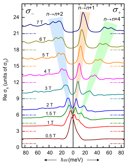
Figure 3: (color online) The theoretical spectra of Re $\sigma_{-}(\omega)$ (on the left) and Re $\sigma_{+}(\omega)$ (on the right) at 5 K at the experimental values of magnetic field. In the calculations, the same parameters were used that give the best fit to the data. The curves are shifted for clarity; the zero levels are shown by dashed-dotted lines of the same color. The peaks corresponding to the fundamental cyclotron resonance $n\rightarrow n+1$ and the most intense harmonics $n\rightarrow n+2$ and $n\rightarrow n+4$ are marked by shaded regions.

The calculated partial optical conductivities due to the high-order resonances $\Delta n=\pm 2$ and $\Delta n=\pm 4$ are shown in Figures 2f-k. The dominant contributions are the electron-like intraband transitions $n\rightarrow n+2$ to $\sigma_{-}(\omega)$ and $n\rightarrow n+4$ to $\sigma_{+}(\omega)$. Although one may expect these overtones to be much weaker than the main cyclotron resonance, they have, in fact, a comparable intensity and form outstanding satellite structures in the total conductivity (Figures 2b,c). Qualitatively, one can relate this very peculiar observation with the comparable values of $\gamma_{3}$ and other interlayer hopping parameters, for example $\gamma_{1}\approx 0.4$ eV. Interestingly, the optical intensities of these two harmonics are about the same, contrary to a naive expectation of having a stronger transition for a smaller $\Delta n$. This can be attributed to the fact that trigonal warping most strongly mixes LLs separated by 3, thus making the harmonics for $\Delta n=3\pm 1$ the strongest and roughly equal in intensity. Our calculations show indeed that the transitions of higher orders (5, 7, etc.) are significantly weaker than the first two harmonics.

Figure 3 presents the evolution of the calculated optical conductivity spectra as a function of the magnetic field. It is evident that the intensities of the transitions $n\rightarrow n+2$ and $n\rightarrow n+4$ are of the same order of magnitude as the one of the transitions $n\rightarrow n+1$ up to at least 7 T and all of them originate from the Drude peak at zero field. In fact, the same calculations (not shown) predict that the high-order harmonics should remain optically visible up to extremely strong fields $\sim$ 100 T. Importantly, such a strong effect of higher harmonics must also exist in multilayer graphene with a similar (Bernal-type) stacking, where trigonal warping is present AbergelPRB07 .

To summarize, we demonstrated that a classical band model, if rigorously applied, describes accurately the cyclotron spectra in graphite in a broad range of magnetic fields. This should serve as a solid basis for the optical investigation of more subtle phenomena such as the coupled electron-hole plasma, electron-phonon interactions and the spin-orbit coupling, the effects essential for the emerging fields of graphite(graphene)-based plasmonics and spintronics. We anticipate that measuring the spectroscopic Kerr angle that allows distinguishing the high-frequency dynamics of electrons and holes without using the circular polarized radiation, will be highly useful in the future studies of the topological insulators, intercalated graphites, multilayer graphene and other materials of fundamental and practical importance. Finally, our work suggests that high-order cyclotron resonances should also be strong in the optical spectra of multilayer graphene up to high fields and therefore should play a major role in the related applications.

This research was supported by the Swiss National Science Foundation by the grants 200021-120347, 200020-135085 and IZ73Z0-128026 (SCOPES program), through the National Center of Competence in Research “Materials with Novel Electronic Properties-MaNEP”. The authors acknowledge useful discussions with L.A. Falkovsky and thank I. Crassee and A. Akrap for critically reading the manuscript.

Decrypting the cyclotron effect in graphite using Kerr rotation spectroscopy: Supplemental Material

Julien Levallois, Michaël Tran and Alexey B. Kuzmenko

Département de Physique de la Matière Condensée, Université de Genève, CH-1211 Genève 4, Switzerland

I Experiment

Magneto-optical measurements were done on a large piece (about 7$\times 7$ mm²) of highly ordered pyrolytic graphite (HOPG) of the ZYA grade, the same as used in Ref. KuzmenkoPRL08, . The misorientation of the z-axis is smaller than 0.4^o as the X-ray rocking curve showed. The sample was mounted in a split-coil superconducting magnet attached to a Fourier-transform spectrometer. A mercury infrared light source, a Ge-coated mylar beamsplitter and a liquid helium cooled bolometer detector were used. The magnetic field was applied along the z-axis perpendicular to the sample and almost parallel to the propagation of light. The average angle of incidence is $8^{\circ}$.

The Kerr rotation angle was determined by placing a rotating grid-wire gold polarizer before the sample and a fixed one just after the sample (before the detector). Without the magnetic field, the signal is at minimum when the two polarizers are crossed. In our configuration the minimum value was less than 1% of the maximum value (when the polarizers are parallel), which allows an accurate polarimetric measurement.

In magnetic field, the minimum shifts by the amount of the Kerr rotation. At every field value, we collected the reflected spectra for a number of polarizer angles around the minimum. The minimum position $\phi_{min}(\omega)$ was then determined as a continuous spectrum. The Kerr rotation is experimentally determined as

$$\theta_{K}(\omega,B)=\phi_{min}(\omega,B)-\phi_{min}(\omega,0),$$ (1)

while the direction of the polarizer rotation was chosen to match the physical definition given by Eq. (1) of the main text. We verified that $\theta_{K}(\omega,-B)=-\theta_{K}(\omega,B)$ within our experimental accuracy. Therefore, in order to reduce the measurement noise, we eventually determined the Kerr angle using the relation:

$$\theta_{K}(\omega,B)=[\phi_{min}(\omega,B)-\phi_{min}(\omega,-B)]/2.$$ (2)

The experimental precision is better than 1 mrad.

The reflectivity of the sample $R(\omega,B)$ was determined using a triple-reference method. First, a ratio of the intensities of a sample ($I_{s}$) and a gold mirror ($I_{r}$) was taken at a given field B:

$$\rho_{(}\omega,B)=I_{s}(\omega,B)/I_{r}(\omega,B).$$ (3)

The switching between the sample and the reference was done with the aid of a computer controlled translation stage. The same ratio $\rho(\omega,0)$ was taken at zero field. The absolute reflectivity was determined using the formula:

$$R(\omega,B)=R(\omega,0)\rho(\omega,B)/\rho(\omega,0),$$ (4)

where $R(\omega,0)$ is the zero field reflectivity, measured on the same sample in a different cryostat allowing an in-situ gold evaporation without displacing the sample KuzmenkoPRL08s . Such a procedure eliminates the sensitivity of the detector to magnetic field, temporal drifts and other systematic uncertainties.

II Theory

In deriving the Landau levels in graphite, we essentially follow the method of Nakao NakaoJPSJ76s ; NakamuraJPSJ76s . The main difference is that instead of adopting the original SWMcC Hamiltonian, we use the tight-binding Hamiltonian with equivalent parameters $\gamma_{0},\gamma_{1},\gamma_{2},\gamma_{3},\gamma_{4},\gamma_{5}$ and $\Delta$, in order to make a direct connection to the recent literature on single- and multilayer graphene CastroNetoRMP09s . The relation between the two Hamiltonians and their parameter sets is given, for example, in Ref. PartoensPRB06s, .

The crystal structure of Bernal stacked graphite is shown in Fig. 1, where also the SWMcC hopping parameters $\gamma_{0},...,\gamma_{5}$ are specified. Due to a strong electronic anisotropy, the band dispersion close to the K-H line is customarily treated by the tight-binding model in the $z$-direction, and by linear expansion in the in-plane momentum ($k_{x},k_{y}$). For each value of $k_{z}$ one can thus define:

$$\tilde{\gamma}_{1,3,4} = 2\gamma_{1,3,4}\cos(k_{z}d/2)$$ (5)

$$\tilde{\gamma}_{2,5} = 2\gamma_{2,5}\cos(k_{z}d)$$ (6)

and write down the $4\times 4$ in-plane Hamiltonian in the {B1, A1, A2, B2} basis:

$$\hat{H}=\left(\begin{array}[]{cccc}\tilde{\gamma}_{2}&\hbar vk_{-}&\hbar\tilde{v}_{4}k_{-}&\hbar\tilde{v}_{3}k_{+}\\ \hbar vk_{+}&\tilde{\gamma}_{5}+\Delta&\tilde{\gamma}_{1}&\hbar\tilde{v}_{4}k_{-}\\ \hbar\tilde{v}_{4}k_{+}&\tilde{\gamma}_{1}&\tilde{\gamma}_{5}+\Delta&\hbar vk_{-}\\ \hbar\tilde{v}_{3}k_{-}&\hbar\tilde{v}_{4}k_{+}&\hbar vk_{+}&\tilde{\gamma}_{2}\end{array}\right)$$ (7)

where $k_{\pm}=k_{x}\pm ik_{y}$, $v=(3/2)(\gamma_{0}a/\hbar)\approx 10^{6}$ m/s is the Fermi velocity and where we also introduced $\tilde{v}_{3,4}=v\tilde{\gamma}_{3,4}/\gamma_{0}$. The last SWMcC parameter $\Delta$ stands for the on-site energy difference between the non-equivalent atomic positions A and B. Here $a$ = 1.43 Å is the carbon-carbon distance and $d$ = 6.7Å̃ is twice the interlayer separation (Fig. 1).

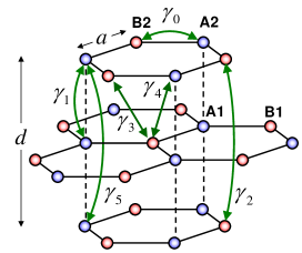
Figure 1: (color online) Crystal structure of Bernal graphite with the indication of the hopping parameters of the SWMcC model.

The velocity operators for the right and the left polarizations can be obtained straightforwardly:

$$\hat{v}_{+}=\frac{1}{\hbar}\frac{\partial{\hat{H}}}{\partial k_{+}}=\left(\begin{array}[]{cccc}0&0&0&\tilde{v}_{3}\\ v&0&0&0\\ \tilde{v}_{4}&0&0&0\\ 0&\tilde{v}_{4}&v&0\end{array}\right),$$ (8)

$$\hat{v}_{-}=\frac{1}{\hbar}\frac{\partial{\hat{H}}}{\partial k_{-}}=\hat{v}_{+}^{*}.$$ (9)

In a perpendicular magnetic field $B$, we make the substitution LuttingerPR55s ; InoueJPSJ62s ; AbergelPRB07s ; FalkovskyPRB11s :

$$k_{-} \rightarrow a^{+}\sqrt{2eB/\hbar}$$ (10)

$$k_{+} \rightarrow a\sqrt{2eB/\hbar},$$ (11)

where $a^{+}$ and $a$ are the ladder operators, acting on harmonic oscillator-like wavefunctions $\psi_{n}$:

$$a\psi_{n} = \sqrt{n}\psi_{n-1}$$ (12)

$$a^{+}\psi_{n} = \sqrt{n+1}\psi_{n+1}.$$ (13)

The Hamiltonian in the operator form reads:

$$\hat{H}=\left(\begin{array}[]{cccc}\tilde{\gamma}_{2}&\epsilon a^{+}&\epsilon_{4}a^{+}&\epsilon_{3}a\\ \epsilon a&\tilde{\gamma}_{5}+\Delta&\tilde{\gamma}_{1}&\epsilon_{4}a^{+}\\ \epsilon_{4}a&\tilde{\gamma}_{1}&\tilde{\gamma}_{5}+\Delta&\epsilon a^{+}\\ \epsilon_{3}a^{+}&\epsilon_{4}a&\epsilon a&\tilde{\gamma}_{2}\end{array}\right),$$ (14)

where we introduced the cyclotron energies:

$$\epsilon = v\sqrt{2e\hbar B}$$

$$\epsilon_{3,4} = \epsilon(v_{3,4}/v).$$

The states $\psi_{0},\psi_{1},...$ form a complete orthogonal basis on one sublattice. As in graphite there are four atoms per unit cell, we add the sublattice index $m=1,2,3,4$ and define the following set of basis states:

$$\Psi_{n}^{m}=\left(\begin{array}[]{c}\delta_{1m}\\ \delta_{2m}\\ \delta_{3m}\\ \delta_{4m}\end{array}\right)\psi_{n}.$$ (19)

It is useful to group them in a particular way NakaoJPSJ76s , namely: $\Gamma_{0}=\{\Psi_{0}^{1}\}$, $\Gamma_{1}=\{\Psi_{1}^{1},\Psi_{0}^{2},\Psi_{0}^{3}\}$ and $\Gamma_{n}=\{\Psi_{n}^{1},\Psi_{n-1}^{2},\Psi_{n-1}^{3},\Psi_{n-2}^{4}\}$ for $n>1$ and arrange in the order $\Gamma_{0},\Gamma_{1},\Gamma_{2},..$. Then the Hamiltonian can be written as a matrix:

$$\hat{H}=\left(\begin{array}[]{cccccc}H_{0}&0&0&G_{0}&0&\cdots\\ 0&H_{1}&0&0&G_{1}&\cdots\\ 0&0&H_{3}&0&0&\cdots\\ G_{0}^{*}&0&0&H_{4}&0&\cdots\\ 0&G_{1}^{*}&0&0&H_{5}&\cdots\\ \vdots&\vdots&\vdots&\vdots&\vdots&\ddots\end{array}\right),$$ (20)

where:

$$H_{0}=\left(\begin{array}[]{c}\tilde{\gamma}_{2}\end{array}\right),H_{1}=\left(\begin{array}[]{ccc}\tilde{\gamma}_{2}&\epsilon&\epsilon_{4}\\ \epsilon&\tilde{\gamma}_{5}&\tilde{\gamma}_{1}\\ \epsilon_{4}&\tilde{\gamma}_{1}&\tilde{\gamma}_{5}\end{array}\right),$$ (25)

$$H_{n=2,3...}=\left(\begin{array}[]{cccc}\tilde{\gamma}_{2}&\epsilon\sqrt{n}&\epsilon_{4}\sqrt{n}&0\\ \epsilon\sqrt{n}&\tilde{\gamma}_{5}+\Delta&\tilde{\gamma}_{1}&\epsilon_{4}\sqrt{n-1}\\ \epsilon_{4}\sqrt{n}&\tilde{\gamma}_{1}&\tilde{\gamma}_{5}+\Delta&\epsilon\sqrt{n-1}\\ 0&\epsilon_{4}\sqrt{n-1}&\epsilon\sqrt{n-1}&\tilde{\gamma}_{2}\end{array}\right),$$ (30)

$$G_{0}=\left(\begin{array}[]{cccc}0&0&0&\epsilon_{3}\end{array}\right),G_{1}=\left(\begin{array}[]{cccc}0&0&0&\epsilon_{3}\sqrt{2}\\ 0&0&0&0\\ 0&0&0&0\end{array}\right),$$ (35)

$$G_{n=2,3...}=\left(\begin{array}[]{cccc}0&0&0&\epsilon_{3}\sqrt{n+1}\\ 0&0&0&0\\ 0&0&0&0\\ 0&0&0&0\end{array}\right).$$ (40)

The Landau levels are calculated by the diagonalization of the matrix (20). In the case $\gamma_{3}=0$ (no trigonal warping) all $G_{n}$ vanish and the Hamiltonian can be factorized into individual blocks $H_{n}$ each of those can be solved separately to provide the sublevels. If $\gamma_{3}\neq 0$ then one has to diagonalize the infinite Hamiltonian, which can be further factorized NakaoJPSJ76s into three independent, although still infinite, matrices by separating subsets $A=\{\Gamma_{0},\Gamma_{3},\Gamma_{6},..\}$, $B=\{\Gamma_{1},\Gamma_{4},\Gamma_{7},..\}$ and $C=\{\Gamma_{2},\Gamma_{5},\Gamma_{8},..\}$. Numerically, the problem can be tackled by truncating an infinite matrix to obtain a finite square matrix $M\times M$ and making $M$ large enough so that increasing it further changes negligibly the energies and the eigenfunctions of the low-index Landau levels of interest. The bands resulting from subsets A, B and C are marked in Fig.2a of the main text by black, red and blue colors respectively.

The velocity operator in the same representation is

$$\hat{v}_{+}=\hat{v}_{-}^{*}=\left(\begin{array}[]{cccccc}0&0&U_{0}&0&0&\cdots\\ V_{1}&0&0&U_{1}&0&\cdots\\ 0&V_{2}&0&0&U_{2}&\cdots\\ 0&0&V_{3}&0&0&\cdots\\ \vdots&\vdots&\vdots&\vdots&\vdots&\ddots\end{array}\right),$$ (41)

where

$$V_{1}=\left(\begin{array}[]{c}0\\ v\\ \tilde{v}_{4}\\ \end{array}\right),V_{2}=\left(\begin{array}[]{ccc}0&0&0\\ v&0&0\\ \tilde{v}_{4}&0&0\\ 0&\tilde{v}_{4}&v\end{array}\right),$$ (49)

$$V_{3,4...}=\left(\begin{array}[]{cccc}0&0&0&0\\ v&0&0&0\\ \tilde{v}_{4}&0&0&0\\ 0&\tilde{v}_{4}&v&0\end{array}\right),$$ (54)

$$U_{0}=\left(\begin{array}[]{cccc}0&0&0&\tilde{v}_{3}\end{array}\right),U_{1}=\left(\begin{array}[]{cccc}0&0&0&\tilde{v}_{3}\\ 0&0&0&0\\ 0&0&0&0\end{array}\right),$$ (59)

$$U_{2,3...}=\left(\begin{array}[]{cccc}0&0&0&\tilde{v}_{3}\\ 0&0&0&0\\ 0&0&0&0\\ 0&0&0&0\end{array}\right).$$ (64)

The circular optical conductivity is calculated using the Kubo formula (the spin and the valley degeneracies are taken into account):

$$\sigma_{\pm}(\omega)=\frac{8e^{3}B}{\pi^{2}}\int_{0}^{\frac{\pi}{d}}dk_{z}\sum_{i,j\neq i}\left|\left\langle i\left|\hat{v}_{\pm}\right|j\right\rangle\right|^{2}$$

$$\times\frac{f(\epsilon_{i})-f(\epsilon_{j})}{\epsilon_{j}-\epsilon_{i}}\frac{i}{\hbar\omega-\epsilon_{j}+\epsilon_{i}+i\Gamma}.$$ (65)

The indices $i$ and $j$ run over all Landau levels at a given $k_{z}$. Here $f(\epsilon)=(1+\exp{(\epsilon-\mu)/T})^{-1}$ is the Fermi distribution function. The chemical potential $\mu$ depends on the magnetic field and can be adjusted using the electrical neutrality condition  KuzmenkoPRB09s :

$$\int_{0}^{\frac{\pi}{d}}dk_{z}\sum_{i}\left[f(\epsilon_{i})-1/2\right]=0.$$ (66)

The optical longitudinal and Hall conductivities are derived from the circular one:

$$\sigma_{xx}(\omega) = [\sigma_{+}(\omega)+\sigma_{-}(\omega)]/2$$

$$\sigma_{xy}(\omega) = [\sigma_{+}(\omega)-\sigma_{-}(\omega)]/2i.$$

In the absence of trigonal warping, only the matrix elements between the levels which quantum numbers $n_{i}$ and $n_{j}$ differ by $\pm$ 1 are non-zero. If $\gamma_{3}\neq 0$ then in principle all transitions are allowed except those where $n$ changes by $0,\pm 3,\pm 6...$, i.e. when both LLs originate from the same subset (A, B or C). As our calculation shows (see the main text) the transitions with $\Delta n=\pm 2$ and $\pm 4$ have the strongest optical intensity, while the others (for example $\Delta n=\pm 5$ and $\pm 7$) are much weaker.

In reality one has to limit the summation to a finite number of LL transitions. Since our goal is to calculate optical properties in a limited spectral range $0<\omega<\omega_{max}$, it is natural to keep only the resonances below a certain threshold value $\Omega>\omega_{max}$. Obviously, the total number of counted transitions then depends on the magnetic field.

The reflectivity and the Kerr angle are given by the formulas

$$R = \frac{|r_{+}|^{2}+|r_{-}|^{2}}{2}$$ (67)

$$\theta_{K} = \frac{\arg(r_{-})-\arg(r_{+})}{2},$$ (68)

where $r_{\pm}$ are the complex reflectivities for the circularly polarized light. At a normal incidence, they are given by the Fresnel equation:

$$r_{\pm}=\frac{1-\sqrt{\epsilon_{\pm}}}{1+\sqrt{\epsilon_{\pm}}},$$ (69)

where

$$\epsilon_{\pm}(\omega)=\epsilon_{\infty}+\frac{4\pi\sigma_{\pm}(\omega)i}{\omega}.$$ (70)

is the in-plane dielectric function. The purpose of the parameter $\epsilon_{\infty}$ is to account for the static dielectric constant associated with all higher-energy optical transitions, not covered by Eq. (65). It should not be considered as a free parameter, since it is determined by the choice of $\Omega$ and can be fixed using the experimentally obtained dielectric function at zero field KuzmenkoPRL08s .

The integration over $k_{z}$ in practice is done by a summation over a finite grid. One has to choose it in such a way that making it denser does not change the result anymore. The optimal density depends on scattering ($\Gamma$), temperature ($T$) and field ($B$).

III Fitting procedure and results

We fitted the Kerr spectra at 1, 3, 5 and 7 T simultaneously with the Equations (68), (69), (70) and (65), by adjusting the SWMcC parameters except $\gamma_{0}$ that we fixed to a value corresponding to $v=1.02\times 10^{6}$ m/s (Ref. OrlitaPRL08s, ). All parameters are assumed to be field-independent. The least-squares criterion was used and the Levenberg-Marquardt fitting routine was employed NumericalRecipess , with an analytical calculation of the derivatives of the output with respect to parameters. The RefFIT software Reffits was used with a dedicated model for graphite. Only a few iterations were needed to achieve a convergence. The best values are presented in Table 2, where also the results of the fitting of recent magnetotransport measurements SchneiderPRL09s are shown, as well as the SWMcC parameters obtained by fitting the calculated bands using the first-principle GW method GruneisPRB08s . One can see that our parameter values agree well with the previous works. The relatively large error bars for $\gamma_{4}$, $\gamma_{5}$ and $\Delta$ are due to the fact that their effects on optical spectra are correlated. By fixing one of them to other experiments, or using magneto-optical data at higher frequencies and magnetic fields LiPRB06s ; TungCM11s we can likely reduce the error bars. However, the main goal of the present work is to demonstrate that the Kerr spectra are fully consistent with the SWMcC model.

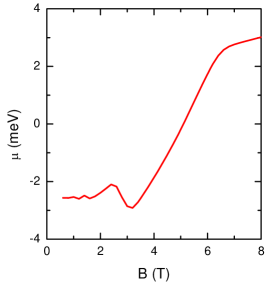
Figure 2: (color online) Magnetic field dependence of the chemical potential.

Fig. 2 shows the dependence of the chemical potential on magnetic field. The non-monotonic dependence is due to the crossing of the Fermi level by the LLs. Almost identical curve is obtained in Ref. SchneiderPRL09s, .

Table 1: SWMcC parameters (in eV) obtained in the present work (1st column), in Ref. SchneiderPRL09s, (2nd column) and Ref. GruneisPRB08s, (3rd column).

	This work	Schneider et al.  SchneiderPRL09s	Gruneis et al. GruneisPRB08s
$\gamma_{0}$	3.16 (fixed)	3.37 $\pm$ 0.02	3.05
$\gamma_{1}$	0.38 $\pm$ 0.01	0.363 $\pm$ 0.05	0.403
$\gamma_{2}$	-0.0089 $\pm$ 0.0003	-0.0121 $\pm$ 0.0005	-0.0125
$\gamma_{3}$	0.297 $\pm$ 0.005	0.31 $\pm$ 0.05	0.274
$\gamma_{4}$	-0.15 $\pm$ 0.1	-0.07 $\pm$ 0.01	-0.143
$\gamma_{5}$	0.005 $\pm$ 0.03	0.025 $\pm$ 0.005	0.015
$\Delta$	0.027 $\pm$ 0.05	0.024 $\pm$ 0.002	0.05
$\Gamma$	0.0028 $\pm$ 0.0002

In the calculations, both $\Omega$ and $\epsilon_{\infty}$ were the same at all fields (0.2 eV and 15 respectively). The size of the truncated matrix $M$ and the number of $k_{z}$ grid points $N_{z}$ was optimized for every field in order to speed up the calculations while keeping a sufficient accuracy. The actual values used are given in Table II.

Table 2: The used computational settings for every field value as explained in the text.

$B$ (T)	0.5	1	1.5	2	3	4	5	6	7
$M$	180	90	60	45	30	24	18	15	15
$N_{z}$	50	100	150	200	300	400	500	600	700

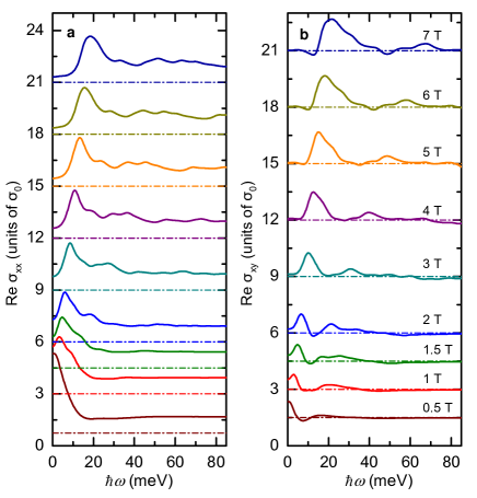
Figure 3: (color online) Real parts of $\sigma_{xx}(\omega)$ (a) and $\sigma_{xy}(\omega)$ (b) that correspond to $\sigma_{\pm}(\omega)$ of Fig.3 of the main text.

For completeness, in Fig. 3 we present the longitudinal and the Hall conductivities obtained from the same calculation (Fig. 3 of the main text).

References

- (1) J. K. Galt, W. A. Yager, and H. W. Dail, Jr., Phys. Rev. 103, 1586 (1956).
- (2) H. Suematsu and S. Tanuma, J. Phys. Soc. Japan. 33, 1619 (1972).
- (3) W. W. Toy, M. S. Dresselhaus and G. Dresselhaus, Phys. Rev. B 15, 4077 (1977).
- (4) R.E. Doezema, W.R. Datars, H. Schaber, and A. Van Schyndel, Phys. Rev. B 19, 4224 (1979).
- (5) K. Nakamura et al., J.Phys. Soc. Japan. 53, 1164 (1984).
- (6) T. Hofmann et al., Rev. Sci. Instr. 77, 063902 (2006).
- (7) Z. Q. Li et al., Phys. Rev. B 74, 195404 (2006).
- (8) M. Orlita et al., Phys. Rev. Lett. 100, 136403 (2008).
- (9) K.-C. Chuang, A. M. R. Baker, and R. J. Nicholas, Phys. Rev. B 80, 161410(R) (2009).
- (10) N. Ubrig et al., Phys. Rev. B 83, 073401 (2011).
- (11) L.-C. Tung, et al., arXiv:1106.5948 (2011).
- (12) V. P. Gusynin, S. G. Sharapov, and J. P. Carbotte, Phys. Rev. Lett. 98, 157402 (2007).
- (13) Z. Q. Li et al., Nature Physics 4, 532 (2008).
- (14) I. Crassee et al., Phys. Rev. B 84, 035103 (2011).
- (15) I. Crassee et al., Nature Physics 7, 48 (2011).
- (16) S. G. Kaplan et al., Phys. Rev. Lett. 76, 696 (1996).
- (17) J.W. McClure, Phys. Rev. 108, 612 (1957).
- (18) J.C. Slonczewski and P.R. Weiss, Phys. Rev. 109, 272 (1958).
- (19) D. S. L. Abergel and V. I. Fal ko, Phys. Rev. B 75, 155430 (2007).
- (20) L.A. Falkovsky, Phys. Rev. B 83, 081107 (2011).
- (21) J. M. Schneider, M. Orlita, M. Potemski, and D.K. Maude, Phys. Rev. Lett. 102, 166403 (2009).
- (22) Z. Zhu et al., Nature Physics 6, 26 (2009).
- (23) A. Gruneis et al., Phys. Rev. B 78, 205425 (2008).
- (24) K. Nakao, J. Phys. Soc. Japan. 40, 761 (1976).
- (25) M. Koshino and T. Ando, Phys. Rev. B 77, 115313 (2008).
- (26) P. Nozieres, Phys. Rev. 109, 1510 (1958).
- (27) M. Inoue, J. Phys. Soc. Japan. 17, 808 (1962).
- (28) M. Mucha-Kruczynski, I.L. Aleiner, V.I. Fal’ko, Phys. Rev. B 84, 041404 (2011).
- (29) A. S. Mayorov et al., Science 333, 860 (2011).
- (30) A. B. Kuzmenko, E. van Heumen, F. Carbone, and D. van der Marel, Phys. Rev. Lett. 100, 117401 (2008).

References

- (1) A. B. Kuzmenko et al., Phys. Rev. Lett. 100, 117401 (2008).
- (2) K. Nakao, J. Phys. Soc. Japan. 40, 761 (1976).
- (3) K. Nakamura et al., J. Phys. Soc. Japan. 53, 1164 (1983).
- (4) A.H. Castro Neto et al., Rev. Mod. Phys. 81, 109 (2009).
- (5) B. Partoens and F.M. Peeters, Phys. Rev. B 74, 075404 (2006).
- (6) J.M. Luttinger and W. Kohn, Phys. Rev. 97, 869 (1955).
- (7) M. Inoue, J. Phys. Soc. Japan. 17, 808 (1962).
- (8) D. S. L. Abergel and V. I. Fal ko, Phys. Rev. B 75, 155430 (2007).
- (9) L.A. Falkovsky, Phys. Rev. B 83, 081107 (2011).
- (10) A. B. Kuzmenko et al., Phys. Rev. B 80, 165406 (2009).
- (11) M. Orlita et al., Phys. Rev. Lett. 100, 136403 (2008).
- (12) W. H. Press, B. P. Flannery, S. A. Teukolsky, and W. T. Vetterling, Numerical Recipes in C, Cambridge Univ. Press (1986).
- (13) A. B. Kuzmenko, Guide to RefFIT: software to fit optical spectra, available online: http://optics.unige.ch/alexey/reffit.html.
- (14) J. M. Schneider et al., Phys. Rev. Lett. 102, 166403 (2009).
- (15) A. Gruneis et al., Phys. Rev. B 78, 205425 (2008).
- (16) Z. Q. Li et al., Phys. Rev. B 74, 195404 (2008).
- (17) L.-C. Tung et al., arXiv:1106.5948 (2011).