Measuring the pulse of GRB 090618: A Simultaneous Spectral and Timing Analysis of the Prompt Emission

Abstract

We develop a new method for simultaneous timing and spectral studies of Gamma Ray Burst (GRB) prompt emission and apply it to make a pulse-wise description of the prompt emission of GRB 090618, the brightest GRB detected in the Fermi era. We exploit the large area (and sensitivity) of Swift/BAT and the wide band width of Fermi/GBM to derive the parameters for a complete spectral and timing description of the individual pulses of this GRB, based on the various empirical relations suggested in the literature. We demonstrate that this empirical model correctly describes the other observed properties of the burst like the variation of the lag with energy and the pulse width with energy. The measurements also show an indication of an increase in pulse width as a function of energy at low energies for some of the pulses, which is naturally explained as an off-shoot of some particular combination of the model parameters. We argue that these model parameters, particularly the peak energy at the beginning of the pulse, are the natural choices to be used for correlation with luminosity. The implications of these results for the use of GRBs as standard candles are briefly described.

1 INTRODUCTION

The phenomenon of Gamma Ray Burst (GRB) has raised many unresolved issues. For example, the nature of the compact object in the progenitor responsible for the jet emission is not yet understood. The widely accepted scenario for the GRB emission, supported by strong observational evidences (van Paradijs et al. 2000), is that of a catastrophic energy release from a highly massive, rapidly rotating, low metallicity star towards the end of its life. This catastrophic process for the long GRB class (T₉₀ $\gtrsim$ 2 s, where T₉₀ is the time taken by the burst to accumulate between 5% to 95% of its prompt emission – see Kouveliotou et al. 1993; Norris et al. 2005) is attributed to the collapsar or hypernova scenario (Woosley 1993; Paczynski 1998; Fryer et al. 1999; Mészáros 2006) while the short GRBs (T₉₀ $\lesssim$ 2 s) are thought of as the outcome of merging neutron star binaries or neutron star-black hole binaries (Paczynski 1986; Meszaros 1992;1997; Rosswog et al. 2003a; b). Though the collapsar model supports the formation of a stellar mass black hole, it is also suggested that the compact object could be a magnetar (Metzger et al. 2007; Metzger 2010).

The prompt emission of long GRBs shows a wide range of structures in their light curve, though the time integrated energy spectra are adequately fit by a four parameter Band model (Band et al. 1993). Attempts have been made to fit the light curve of the prompt emission with empirical models such as the Fast Rise Exponential Decay (FRED) model (Kocevski et al. 2003) and the exponential model (Norris et al. 2005). These models assume an underlying pulse structure of the prompt emission. The curve fitting shows that the pulses are nearly simultaneous in a wide range of energy bands (Norris et al. 2005) and have self similar shapes (Nemiroff 2000). Hakkila et al. (2011) showed that the observed properties of the short pulses of long GRBs correlate the same way as typical pulses of short GRBs. All these properties of pulse emission indicate that despite being diverse in their many features, the prompt emission of GRB has a simple underlying mechanism of pulse emission which can be characterized by empirical models irrespective of the progenitor or the environment of its formation (Hakkila et al. 2011).

The properties of the prompt emission of GRBs like $E_{peak}$ (the energy at which the emission peaks – Amati et al. 2002), the lag between the light curves at two energies (Norris et al. 2000), the average variability seen during the prompt emission (Fenimore & Ramirez-Ruiz 2000), the rise time of the pulses (Schaefer 2002) are found to be correlated to the luminosity of the bursts and hence they are used as distance indicators (Schaefer 2007; Gehrels et al. 2009). Most of these derived relations are empirical in nature and the analyses that are done to derive these parameters, however, are done separately in the time or the energy domain. For example, to derive $E_{peak}$ the time-integrated spectrum is used, ignoring the time variability and the pulse characteristics. Similarly, to derive lags, the time profile is examined in a few broad energy bands. Attempts have been made to investigate the variations of these derived parameters in the other domain. For example, the variation of $E_{peak}$ with time has been investigated by Kocevski & Liang (2003). A complete empirical description of GRB prompt emission which describes the time as well as energy distribution, however, is lacking. This is probably due to the method of spectral parameter determination which is forward in nature: that is one assumes a possible spectral model, convolves with the detector response and verifies the validity of the model by comparing with the data (Arnaud 1996). Hence it is difficult to incorporate time variability parameters in this scheme. GRBs often have overlapping pulses which further complicates the extracting of model parameters for any unified empirical description.

In this paper we develop a technique to give a complete pulse-wise empirical description of the prompt emission of a GRB using the time-integrated spectrum and the energy integrated light curve. We apply this method to the Fermi/GBM and the Swift/BAT data of GRB 090618, which has the highest fluence among all 438 GBM GRBs until March 2010 (Nava et al. 2011). We exploit the large area of Swift/BAT to get accurate light curves and the large band-width of Fermi/GBM to get accurate energy spectra. We use the Band description for the time integrated spectral model (Band 2003) and the exponential model (Norris et al. 2005) for the energy integrated timing description for the pulses. We use the expression for the variation of $E_{peak}$ with time given by Kocevski & Liang (2003) and develop a method to derive the model parameters (see section 4.1.2). We demonstrate that these model parameters correctly describe the variation of pulse width with energy and the variation of the lag with energy.

In §2 we give a brief description of GRB 090618, and in §3 we give the data analysis techniques including spectral analysis (§3.1), timing analysis (§3.2) and a pulse-wise joint (Swift/BAT and Fermi/GBM) spectral analysis (§3.3). In §4 we describe our method in detail, which gives a complete three dimensional pulse-wise description of the GRB. The model predicted timing results are compared with the observations in §4.2 and the implications for global correlations are touched upon in §4.3. The results are discussed and the major conclusions are given in the last section (§5).

2 GRB 090618

The brightest Gamma Ray Burst (GRB) in the Fermi era (as of March 2010), GRB 090618, was simultaneously observed with Swift/BAT (Schady et al. 2009a; 2009b; 2009c), AGILE (Longo et al. 2009), Fermi/GBM (McBreen et al. 2009), Suzaku/WAM (Kono et al.), Wind/Konus-Wind, Coronas-Photon/Konus-RF (Golenetskii et al. 2009), Coronas-Photon/RT-2 (Rao et al. 2009; 2011). This is a long GRB (T₉₀$\sim$113 s) with a fluence of $3398.1\pm 62.0\times 10^{-7}$ erg/cm² (integrated over $\triangle t$=182.27 s). The detection time reported by Swift/BAT is 2009 June 18 at 08:28:29.85 UT (Schady et al. 2009a) whereas the Fermi/GBM detection time is 08:28:26.66 UT (McBreen et al. 2009). This burst showed structures in the light curve with four peaks along with a precursor. A significant spectral evolution was also observed in the prompt emission which lasted for about 130 s from the trigger time (for a summary see Rao et al. 2011).

The GRB afterglow was observed in the softer X-rays and optical regions. The optical afterglow was tracked by Palomar 60-inch telescope (Cenko 2009), Katzman Automatic Imaging Telescope (Perley et al. 2009) followed by various other optical, infrared, and radio observations. Observations using the Kast spectrograph on the 3-m Shane telescope at Lick Observatory (Cenko et al. 2009) revealed a redshift of z = 0.54 (Cenko et al. 2009a). The X-ray afterglow was measured by the Swift/XRT (Schady et al. 2009b). Initially very bright in the X-rays, the flux rapidly decayed with a slope of $\sim$6 before breaking after 310 s from the trigger time when the burst entered a shallower decay phase (slope 0.71$\pm$0.02 – Beardmore et al. 2009).

Rao et al. (2011) analyzed the prompt emission of GRB 090618 using Coronas-Photon/RT-2 and Swift/BAT data. The light curves in various energy bands were fitted with a FRED profile to identify pulse characteristics such as width, peak position etc. A joint RT-2 and BAT spectral analysis of individual pulses was done using the spectral model of Band. The reported time integrated low energy photon index $\left(\alpha\right)$, the high energy photon index $\left(\beta\right)$, and the peak energy $\left(E_{peak}\right)$ are -1.40, -2.50, and 164 keV, respectively. Ghirlanda et al. (2010) performed a time resolved spectral analysis of Fermi GRBs of known redshifts (GRB 090618 being one of the twelve in the list) to show that the time-resolved correlation $\left(E_{peak}^{t}-L_{iso}^{t}\right)$ within individual GRBs is consistent with time-integrated correlation $\left(E_{peak}-L_{iso}\right)$ indicating that there must be a physical origin for the correlation and may not be an outcome of instrumental selection effects.

3 DATA ANALYSIS

We used Fermi/GBM and Swift/BAT data for our analysis. The GBM consists of twelve Sodium Iodide (NaI: nx where x runs from 0 to 11) and two Bismuth Germanate (BGO : by, where y runs from 0 to 1) detectors. The NaI covers the energy range $\gtrsim$ 8 keV to $\sim$ 1 MeV while the BGO covers a wider range of $\sim$ 200 keV to $\sim$ 40 MeV. Data are saved in three types of packets (Meegan et. al. 2009): (1) TTE (Time Tag Events) in which time and energy information (in 128 energy channels) of individual photons are stored, (2) CSPEC: binned data in 1.024 s bins and 128 energy channels and (3) CTIME: binned data in 0.064 s bins and 8 energy channels (which is not suitable for spectroscopy). The triggered detectors for the GRB 090618 were n4, n7, b0, and b1. In the following analysis we have used n4, n7 and either b0 or b1, one at a time. On the other hand, BAT has an array of CdZnTe detector modules located behind a Coded Aperture Mask. This covers an energy range of 15 keV to 150 keV (Barthelmy et al. 2005; Gehrels et al. 2004). The large area of BAT (5200 $\rm cm^{2}$) gives very good sensitivity for timing analysis, compared to that of NaI/BGO (126 $\rm cm^{2}$) detectors of GBM.

3.1 Spectral Analysis

Ghirlanda et al. (2010) have presented the time resolved spectral analysis results for GRB 090618 in 14 time segments. We essentially followed the same methodology, but have also used the simultaneous Swift/BAT data. GRB 090618 triggered the Swift/BAT instrument on 2009-06-18 at 08:28:29.851 or 267006514.688 MET (s). The Fermi/GBM trigger time is $T_{0}$(GBM) = 2009-06-18 08:28:26.659 UT or 267006508.659 MET (s). Hence there is a delay time in the BAT data file which must be subtracted during the joint analysis. The calculated time delay is -3.192 s and when we convert it to MET it gives 267006511.496 MET (s) for Swift/BAT. In all the analysis this time is subtracted from the trigger time unless specified otherwise.

For the GBM we chose the TTE (Time Tag Event) files of the triggered NaI detectors, namely n4 and n7. The BGO detector was excluded as it is not suitable for time resolved spectroscopy due to its lower sensitivity (Ghirlanda et al. 2010). The energy range was chosen to be $\gtrsim$ 8 keV to $\sim$ 900 keV. We used RMFIT package provided by the

Figure 1: Comparison of the parameters obtained from a time resolved spectral analysis of the prompt emission of GRB 090618 using a cut-off power law model. The left panel shows the power law indices obtained from a joint GBM and BAT analysis plotted against those obtained from a GBM analysis. The right panel shows a similar plot for the cutoff energy $E_{0}$. In both cases the straight line has a slope 1 denoting the equality of measurements ($-\alpha$ is plotted for convenience).

User Contributions of Fermi Science Support Center (FSSC) to select the desired time cuts and for generating the background files. The background was taken before and after the burst, avoiding burst contamination (Ghirlanda et al. 2010) and the exposure time for background was optimized for different detectors. The energy channels were binned so as to get a minimum of 40 counts per channel. For the analysis of the BAT data we used standard tasks prescribed in The Swift BAT Software Guide, Version 6.3 of Heasoft 6.9 employing a time delay of -3.192 s.

These spectra were then fitted with a cut-off power law of the form $F=cons\times E^{\alpha}exp(-E/E_{0})$ where F is the photon flux. The constant factor, cons, was kept free while fitting essentially to take care of the different systematic errors in the area calibration of the two instruments. The derived parameter values (using GBM alone) were found to be consistent with the values presented in Ghirlanda et al. (2010). Figure 1 shows the comparison results of the spectral analysis. In Figure 1 (left panel) the indices $\alpha$ obtained from the joint analysis are plotted against those obtained from an analysis of the GBM data for the fourteen different time segments. Similar data for the parameter $E_{0}$ are shown in the right panel. A deviation is noted for the parameter $\alpha$ in the 0 to 3 s region. This may be attributed to lower count rate of BAT in the precursor region.

We note a systematic increment in the value of $\alpha$ and $E_{0}$ after the inclusion of BAT data. Further, the constant factor is always lower by 10-20% for the BAT. Sakamoto et al. (2011) have made a joint spectral analysis of 14 GRBs using data from Swift/BAT, Konus/Wind and Suzaku/WAM and they have noted that for the BAT data, the constant factor is systematically lower by 10 – 20%, the photon index is steeper by 0.1 – 0.2 and the $E_{peak}$ becomes higher by 10 – 20%. The results presented here are in general agreement with these conclusions.

In Figure 2 we have plotted the ratio of fractional errors as a function of the measured parameters. We find that there is a marginal improvement for the parameter $E_{0}$ (Figure 2, right panel). The parameter $\alpha$ (Figure 2, left panel), however is measured always with a greater accuracy from the joint analysis. The large effective area of BAT improves the accuracy of the spectral index whereas its low high energy threshold ($\sim$150 keV) makes relatively low impact on the measurement of the high energy cut-off value. The joint analysis always gives confidence on the measured parameters and ensures that the effects of instrumental artefacts are minimized. Hence we use, in the later analysis, a joint fit for measuring the global spec-

Figure 2: The ratio of fractional errors for GBM-BAT joint analysis to the GBM analysis is shown as a function of the measured values of $\alpha$ (left panel) and $E_{0}$ (right panel) obtained from a fitting for GBM data alone. The dotted line in both cases shows the average of all errors measured. This is found to be marginally less than the line of equal error (dot dashed) for the $E_{0}$ and well below that line for $\alpha$ measurement ($-\alpha$ is plotted for convenience).

tral parameters and use only the BAT data for a joint timing and spectral analysis.

3.2 Timing Analysis

We identified four pulses (other than the precursor) in the $\sim$60 s to $\sim$130 s period after the trigger. Both the Swift/BAT and Fermi/GBM (n4) were used for the timing analysis. We subtracted background and shifted the time origin to the trigger time (TRIGTIME is the keyword in the header) of the respective satellite. As we noted previously, there is a time lag of -3.192 s for the BAT trigger. Light curves were extracted for different energy bands for both the data sets. The energy bands for the Swift/BAT were: 15-25 keV, 25-50 keV, 50-100 keV, and 100-200 keV. For the Fermi/GBM (n4) we chose 8-15 keV, 15-25 keV, 25-50 keV, 50-100 keV, 100-200 keV, and 200-500 keV. Greater than 500 keV region of NaI and the BGO detector of GBM were excluded because the third and the fourth pulses were not detected in these bands.

All the light curves were fitted with the four-parameter model of Norris et al. (2005)

$$I(t)=A_{n}\lambda exp\{-\tau_{1}/(t-t_{s})-(t-t_{s})/\tau_{2}\}$$ (1)

for $t>t_{s}$, where $\mu=\left(\tau_{1}/\tau_{2}\right)^{\frac{1}{2}}$ and $\lambda=exp\left(2\mu\right)$. $A_{n}$ is the pulse amplitude, $t_{s}$ is the pulse start time and $\tau_{1}$, $\tau_{2}$ are time constants characterizing the rise and decay part of the pulse. From these parameters, various derived quantities like the peak position, the pulse width (measured as the separation between the two 1/e intensity points), and the pulse asymmetry can be calculated (see Norris et al. 2005 for details). Errors are calculated for the parameters as nominal 90% confidence level errors ($\triangle\chi^{2}$=2.7) and these errors are propagated for the derived quantities, as described in Norris et al. (2005).

Figure 3 shows the pulse width (w) as a function of energy (E) for all the pulses. Apart from the fact that the width broadens in the lower energy bands, we note a tentative evidence for a decrement (or constancy within error bar) of the width from 50-100 keV through 8-15 keV energy bands for the third and the fourth pulses (lower panels of Figure 3). We fitted these data for the individual pulses with (i) constant ($w=c$) and (ii) linear ($w=mE+c$) models. For the first two pulses there was a significant improvement in the $\chi^{2}$ for a linear fit (the $\chi^{2}$ varied from 16.2(9) to 5.1(8) and 140.9(9) to 7.9(8) respectively for the two pulses; the numbers in the brackets are the degrees of freedom). The derived slopes are $(-7.4\pm 2.6)\times 10^{-3}$ s $\rm keV^{-1}$ and $(-5.5\pm 0.4)\times 10^{-3}$ s $\rm keV^{-1}$, respectively for the two pulses. The third and the fourth pulses, however, showed negligible improvement in

Figure 3: Pulse width (w) is plotted against energy (E), for pulse 1 to 4 respectively in the top to bottom panels. The fourth pulse is insignificant in the 200-500 keV energy range. Hence the fourth panel has a different scale on the x-axis.Values derived from the Swift/BAT and the Fermi/GBM data are shown by circles and filled circles, respectively. While the width decreases with increasing energy for the first two pulses (top two panels), there is a tentative evidence of the reverse effect in the lower energy ($\sim$ 10-70 keV band) for the other two pulses (see section 3.2).

$\chi^{2}$ (from 8.7(9) to 6.0(8) and 2.1(8) to 2.1(7), respectively for the two pulses) for the linear fit. For these two pulses, when the data below 70 keV is considered, there is a marginal improvement in the $\chi^{2}$ for a linear fit with a positive slope (from 8.7(9) to 3.8(5) and 2.1(8) to 1.5(5), respectively for the two pulses). The derived slopes are $(15\pm 14)\times 10^{-3}$ s $\rm keV^{-1}$ and $(10\pm 21)\times 10^{-3}$ s $\rm keV^{-1}$ respectively. Though the slopes for these two pulses are positive, the error bars are quite large and hence the evidence of this reverse variation is tentative. In Figure 3 (lower two panels) the linear fit for pulse 3 and 4 are shown by solid lines (in the low energy) and dot-dashed lines (in full energy band). We have ignored the fourth pulse in the 200-500 keV band of Fermi for the fitting as it was not prominent in this energy band.

3.3 Pulse-Wise Joint Spectral Analysis

The peak position and the width gave a clue for the time cut for each pulse and facilitated the selection of integration time for pulse spectral analysis of the individual pulses. The pulse spectral analysis was done with a Band function fit and including the BGO detector of GBM. We included the precursor pulse in this analysis. We divided the GRB event into four time segments namely, Part 1 ($T_{0}$ to $T_{0}+50$), Part 2 ($T_{0}+50$ to $T_{0}+77$), Part 3 ($T_{0}+77$ to $T_{0}+100$) and Part 4 ($T_{0}+100$ to $T_{0}+180$). The first and second pulses are considered together as there is too much overlap between them.

All the spectra were fitted in the energy range $\sim$ 8 keV - $\sim$ 1 MeV with the four parameter model of Band (Band et al. 1993):

$$I(E)=\left\{\begin{array}[]{ll}A_{b}\left[\frac{E}{100}\right]^{\alpha}exp\left[\frac{-(2+\alpha)E}{E_{peak}}\right]\\ \\ $\rm if$\leavevmode\nobreak\ \leavevmode\nobreak\ E\leq[(\alpha-\beta)/(2+\alpha)]E_{peak}\\ \\ A_{b}\left[\frac{E}{100}\right]^{\beta}exp\left[\beta-\alpha\right]\left[\frac{\left(\alpha-\beta\right)E_{peak}}{100\left(2+\alpha\right)}\right]^{(\alpha-\beta)}\\ \\ otherwise\end{array}\right.$$ (2)

The lower and the higher energy parts are characterized by the parameters $\alpha$ and $\beta$ respectively and they meet smoothly at the spectral break energy $[(\alpha-\beta)/(2+\alpha)]E_{peak}$. The peak energy, $E_{peak}$ or equivalently the characteristic energy, defined as $E_{0}=E_{peak}/\left(2+\alpha\right)$, may be considered as the third parameter of the model. The best fit model parameters along with the nominal 90% confidence level error ($\triangle\chi^{2}$=2.7) for the joint fit of Fermi/GBM (n4, n7, b1) and Swift/BAT are reported in Table 1 (b0 in place of b1 gives similar results). The high energy photon index $\beta$ is constrained primarily by the GBM data and hence we have kept its value fixed at -2.5 to determine precise values of $E_{peak}$ and $\alpha$. Only in one case namely for the full range ($T_{0}$ to $T_{0}+180$ sec) of the GRB, $\beta$ was made to vary and a value of -2.96 was obtained. Figure 4 shows the joint Band spectral fitting of this range along with the $\chi^{2}$ deviation of the data.

An examination of the residuals in Figure 4 reveals that there are some systematic differences in the response in the 20-40 keV region between BAT and GBM data and the resultant $\chi^{2}$

Table 1: spectral parameters of GRB 090618 for Band model, from a joint analysis of Fermi/GBM (n4, n7, b1) and Swift/BAT data

Part	$\alpha$	$\beta$	$E_{peak}$(keV)	$\chi^{2}$(dof)	$E_{0}$ (keV)
Full	-1.35$\pm 0.02$	-2.5 (fixed)	154$\pm 7$	428(299)	236$\pm 18$
Part 1 (Precursor)	-1.25$\pm 0.05$	-2.5(fixed)	$166_{-14}^{+18}$	369(299)	$221_{-33}^{+39}$
Part 2 (Pulse 1 & 2)	-1.11$\pm 0.02$	-2.5(fixed)	212$\pm 9$	460(299)	238$\pm 15$
Part 3 (Pulse 3)	-1.15$\pm 0.03$	-2.5(fixed)	114$\pm 4$	334(259)	134$\pm 9$
Part 4 (Pulse 4)	$-1.65_{-0.08}^{+0.11}$	-2.5(fixed)	33$\pm 3$	431(299)	$94_{-30}^{+38}$
Full (free $\beta$)	-1.36$\pm 0.02$	-2.96$\pm$0.48	$160_{-8}^{+9}$	418(288)	$250_{-20}^{+22}$

Figure 4: Fitting of Band function to the full range (0 to 180 s) of GRB 090618 for the energy range $\sim$ 8 keV to $\sim$ 1 MeV. The range of the BGO detector starts above 200 keV, while BAT covers up to $\sim$ 150 keV. The other two detectors namely n4 and n7 have the spectrum above 8 keV to $\sim$ 800 keV. The extreme channels and specifically the 25th channel of n4 are ignored due to high background rates. The unfolded spectrum of BAT shows a lower normalization (see text).

values generally are quite high. The resultant spectral parameters, however, agree with the results reported for this GRB (Ghirlanda et al., 2010; Nava et al. 2011; Rao et al. 2011). The errors are significantly better compared to the joint BAT and RT-2 analysis (Rao et al. 2011), but comparable to that obtained from a GBM analysis alone (Nava et al. 2011). Since a joint analysis using data from different satellites pins down the systematic errors in each instruments, we believe that the joint analysis results, reported here, are devoid of instrumental artefacts, particularly for the parameters $\alpha$ and $E_{peak}$.

4 JOINT SPECTRAL AND TIMING STUDY: AN ALTERNATE APPROACH

4.1 Two Parameter XSPEC Table Model

4.1.1 The time evolution of $E_{peak}$

The light curve of each pulse of a GRB can be described in terms of the four-parameter model of Norris (equation 1) and the spectrum for each pulse can be fitted with the Band model (equation 2). Liang and Kargatis (1996) showed for clean, separable pulses that the peak energy of the $\nu F_{\nu}$ spectrum, $E_{peak}$, decays with the photon fluence as,

$$E_{peak}(t^{\prime})=E_{peak,0}\leavevmode\nobreak\ e^{-\phi(t^{\prime})/\phi_{0}}$$ (3)

where $E_{peak,0}$ is the peak energy at zero fluence, $\phi_{0}$ is the decay constant and $t^{\prime}=t-t_{s}$. The quantity $\phi(t^{\prime})$ is the fluence up to time t from the start of the pulse ($t_{s}$). For convenience of description we shift our origin to $t_{s}$ and hence $t^{\prime}=t$ for each pulse analysis. Equation 3 quantifies the overall softening of the burst with time.

Kocevski and Liang (2003) have integrated the light curves of a sample of GRBs up to various times t and found the fluence, $\phi(t)$, at those times. The peak energy at the same times, $E_{peak}(t)$, were found by fitting the spectra with a Band model. They determined the $E_{peak,0}$ and $\phi_{0}$ from a semi-log plot of $E_{peak}(t)$ versus $\phi(t)$ and fitting a straight line. This procedure was adopted for clean, bright, and separable FRED pulses.

Here we explore a method to determine the timing and spectral parameters by assuming that $E_{peak}(t)$ and $\phi(t)$ are related according to equation 3 in each pulse. Essentially we assume that for each pulse, the variation of flux with time is given by the exponential model (equation 1), and at each time the spectra is described by a Band function (equation 2), and, for a given pulse, only the peak energy varies with time governed by equation 3. We develop a method to derive the model parameters from a time integrated spectrum and energy integrated light curve.

4.1.2 Description of the method

The flux of a GRB pulse is a function of time and energy. If there exist empirical formulae for the temporal and spectral beahvior then the flux can be described in terms of all the model parameters. For example, the variation of flux with time is given by Norris’ exponential model, with four parameters ($A_{n}$, the normalization, $t_{s}$, $\tau_{1}$, and $\tau_{2}$). The spectral behaviour is parametrized by a Band function, with four parameters ($A_{b}$, the normalization, $\alpha$, $\beta$, and $E_{peak}$). For any timing model, the time parameters change with energy e.g., the derived parameter, width, changes in various energy bands (see section 3.2). Similarly, the spectral parameters of any spectral model change with time e.g., $\alpha$ and $E_{0}$ of cut-off power law change with time in the same pulse (see section 3.1).

The Norris exponential model (equation 1) describes the evolution of a pulse with time. This description can be used for counts in any energy band and the variation of the model parameters with energy can be studied. Instead, we assume that the model parameters $\tau_{1}$ and $\tau_{2}$ derived for a pulse integrated over all energy bands are global parameters describing the evolution of total flux with time. Since the variation of spectrum is best described by the peak energy evolution with fluence (equation 3), we further assume that $\alpha$ and $\beta$ do not change with time. The normalization factors ($A_{n}$ and $A_{b}$) are related by the fact that the fluence calculated either by time integration of the pulse light curve or by the integration over the total energy should be the same. With these assumptions, the parameters for a given pulse are determined as follows.

Table 2: Best fit values of $E_{peak,0}$ and $\phi_{0}$ for the pulses as determined by the $\chi^{2}$ minimization of the spectral data with the additive table model. The first two pulses are combined together. The other pulse characteristics ($\tau_{1}$, $\tau_{2}$, and $t_{s}$) are also reported.

Pulse	$E_{peak,0}$	$\phi_{0}$	Norm	$\chi^{2}$ (dof)	$\tau_{1}$(s)	$\tau_{2}$(s)	$t_{s}$(s)
1	$359_{-92}^{+65}$	$12.2_{-1.3}^{+2.5}$	$0.74\pm 0.06$	40.12 (75)	$795.4_{-7.1}^{+7.2}$	$0.54_{-0.005}^{+0.005}$	$40.1_{-0.2}^{+0.2}$
2					$858.2_{-7.7}^{+6.4}$	$0.58_{-0.005}^{+0.004}$	$44.2_{-0.2}^{+0.2}$
3	$324_{-83}^{+82}$	$18.8_{-6.2}^{+9.6}$	$0.54\pm 0.04$	31.41 (75)	$353.4_{-50}^{+43}$	$2.47_{-0.09}^{+0.12}$	$50.3_{-1.2}^{+1.5}$
4	$307_{-99}^{+41}$	$12.0_{-2.1}^{+2.0}$	$0.19\pm 0.04$	56.42 (75)	$532.0_{-132}^{+209}$	$1.58_{-0.16}^{+0.15}$	$81.0_{-3.4}^{+2.6}$

For a given pulse, we use the energy integrated light curve from BAT and use equation 1 for the fitting. This best fit light curve is used to determine the global parameters namely, $A_{n}$, $\tau_{1}$, and $\tau_{2}$. Since we can arbitrarily choose the pulse starting time by shifting the time origin, the parameter $t_{s}$ is not very relevant (also see section 4.1.1). This function is then integrated up to a time t to determine $\phi(t)$. From the individual spectral fitting for each pulse using the Band model, $\alpha$ and $\beta$ are determined (see section 3.3). Now, if the constant parameters namely, $E_{peak,0}$ and $\phi_{0}$ are determined, we have a complete spectral and timing description of a GRB pulse. For this purpose, we use a two-dimensional grid of guess values for these two parameters and then determine the best fit values by a spectral fitting method.

For a particular combination of $E_{peak,0}$ and $\phi_{0}$ values, $E_{peak}(t)$ at any time t can be determined from equation 3. On the other hand, equation 2 can be rewritten as $I(E)=A_{b}\leavevmode\nobreak\ f(E)$ where $A_{b}$ is the normalization and f(E) is the rest of the functional form valid in the two energy bands. Given the global parameters ($\alpha$ and $\beta$) and the time dependent parameter ($E_{peak}(t)$), f(E) can be determined. The normalization $A_{b}(t)$ can be found by dividing the fluence ($\phi$(t)) of the light curve by the f(E) integrated over the whole energy range. Hence photon spectrum is generated for the time instance t. Choosing a time and energy grid, counts can be plotted as a function of time and energy for a particular combination of $E_{peak,0}$ and $\phi_{0}$ values, and the resulting surface can be referred to as a three dimensional pulse model. Hence for a two-dimensional grid of guess values of $E_{peak,0}$ and $\phi_{0}$ we can generate three dimensional pulse models for each of the grid points. These model pulses can be used in two ways: (1) integration over time gives the model spectrum of that pulse, (2) integration over various energy bands gives model light curves of that pulse in those energy bands.

In our analysis, we first generate a two parameter XSPEC table model using the guess values of $E_{peak,0}$ and $\phi_{0}$ and then use this table model to determine the best fit values of these two parameters by fitting the time integrated spectrum (see section 4.1.3). With this method, we get a complete description of the pulse with model parameters determined from the data.

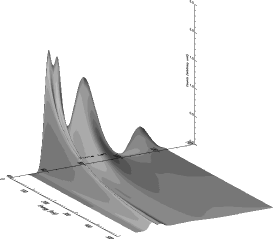
Figure 5: The three dimensional model of the whole GRB using a model with the best fit values of $E_{peak,0}$ and $\phi_{0}$ for each pulse. Counts in arbitrary unit is plotted in the vertical axis against time and energy. The pulses are shifted to original pulse start time (see Table 2).

Using this model we can reconstruct the three dimensional pulse profiles and can generate light curves in any energy band. Various timing parameters (width and lag) are derived in these energy bands (see section 4.2) and these model predicted values can be compared with the observed values to get a validation of the whole procedure.

4.1.3 Specification of the table model and the best fit values

For all the pulses we use a time grid resolution of 0.5 s and energy grid resolution of 2.0 keV. Each pulse has a separate XSPEC table model, though the first and second pulses are combined together as the data overlap. A typical table model contains a spectrum in the 2-200 keV energy range for 200 values of $E_{peak,0}$ from 100.0 keV to 1100.0 keV and 50 values of $\phi_{0}$ from 2.0 photon $\rm cm^{-2}$ to 77.0 photon $\rm cm^{-2}$, energy binning information, parameter values and the required header keywords standardized as per the requirement by XSPEC described in OGIP Memo OGIP/92-009.

The additive table model is used to determine the best fit values of $E_{peak,0}$ and $\phi_{0}$ by the standard $\chi^{2}$ minimization procedure. The best fit values with nominal 90% confidence errors are reported in Table 2. The parameters, $E_{peak,0}$ and $\phi_{0}$ of the first two pulses are assumed to be the same. It should be noted here that we have used the normalization $A_{n}$ as a global parameter to calculate $\phi$(t). The normalization of the subsequent pulse profile is derived from the integration of f(E) over the total energy band (see section 4.1.2). Effectively this leads to a spectrum with normalization

(a)

(b)

Figure 6: Observed light curve in the full energy range 15-200 keV fitted with the Norris’ exponential model is shown in the left panel. The timing parameters are determined and used in the pulse generation to predict light curves in all energy bands. One such predicted light curve in the 25-50 keV region is shown along with the observed light curve in the right panel. The count/s in the y-axis is BAT mask weighted count $\rm s{-1}$.

as a free parameter. This normalization is determined during the spectral fitting using XSPEC, and is also reported in Table 2.

4.1.4 Three dimensional pulse model for the best fit values

Three dimensional model of each pulse is generated for the best fit parameter values (as described in sections 4.1.2 and 4.1.3). The three dimensional model of the whole GRB obtained from the sum of these models of the pulses with each pulse shifted to its proper starting time is shown in Figure 5. This figure is used only for display purposes. In actual analysis, each pulse is normalized properly, before calculating various parameters as the overall normalization may vary for each pulse. This normalization is achieved for spectrum and light curve separately.

4.2 Timing analysis using the model

4.2.1 Reproducing the light curves

Once we get the best fit values of $E_{peak,0}$ and $\phi_{0}$ for each pulse we can generate the best fit model light curve by integrating the three dimensional pulse model for the best fit value over the desired energy range. We generate three dimensional pulse models, shift them over appropriate starting time, co-add them with proper normalization factors and integrate over energy ranges to generate the combined light curves in the energy bands: 15-25 keV, 25-50 keV, 50-100 keV and 100-200 keV of BAT. In Figure 6 (right panel), we show the observed light curve along with the model predicted light curve for the 25-50 keV energy band. In the left panel Norris’ exponential model fit for the total energy range is shown. Parameters from this fit (Figure 6, left panel) were used for characterizing the timing parameters in our model.

The GRB light curve shows rapid time variable components over and above the smooth pulse structure. In the pulse description we consider only this smooth variation. Any small rapid time variability in the data gives large value of $\chi^{2}$ when we use the smooth pulse model for fitting. Hence, the normalization factor could not be determined by $\chi^{2}$ minimization. Instead we physically examined the heights and determined the normalization. The co-added pulses reproduce the light curve quite well. Hence, we can conclude that the total light curve and the integrated spectrum, with the assumption of $E_{peak}(t)$ varying with $\phi(t)$ in a predetermined way (equation (3)), correctly reproduces the energy resolved light curves. This can be taken as a confirmation of the assumption of the $E_{peak}$ variation. It should, however, be noted that

Table 3: Variation of the model predicted width of each pulse with energy. Numbers within brackets are the measured pulse widths.

Pulse	15-25 keV	25-50 keV	50-100 keV	100-200 keV
1	$6.05_{-0.12}^{+0.12}$ ($6.74_{-0.13}^{+0.13}$)	$5.88_{-0.16}^{+0.16}$ ($6.67_{-0.39}^{+0.39}$)	$5.54_{-0.17}^{+0.16}$ ($6.18_{-1.62}^{+1.62}$)	$5.08_{-0.18}^{+0.15}$ ($5.79_{-0.30}^{+0.30}$)
2	$6.56_{-0.19}^{+0.22}$ ($7.52_{-0.13}^{+0.13}$)	$6.35_{-0.19}^{+0.22}$ ($7.40_{-0.04}^{+0.04}$)	$5.89_{-0.34}^{+0.27}$ ($7.23_{-0.11}^{+0.11}$)	$5.33_{-0.34}^{+0.20}$ ($6.82_{-0.04}^{+0.04}$)
3	$17.84_{-0.70}^{+0.47}$ ($18.01_{-3.91}^{+3.91}$)	$18.10_{-0.89}^{+0.53}$ ($18.09_{-0.40}^{+0.40}$)	$18.68_{-0.96}^{+0.74}$ ($17.22_{-1.43}^{+1.43}$)	$19.82_{-0.64}^{+0.49}$ ($15.87_{-1.63}^{+1.63}$)
4	$14.45_{-0.92}^{+0.99}$ ($13.32_{-0.51}^{+0.51}$)	$14.66_{-0.96}^{+0.98}$ ($13.76_{-1.60}^{+1.60}$)	$15.18_{-0.88}^{+0.62}$ ($14.00_{-1.23}^{+1.23}$)	$15.93_{-1.27}^{+1.16}$ ($13.03_{-1.84}^{+1.84}$)

a single joint spectral fit is done for pulses 1 and 2 and hence the derived values of $E_{peak,0}$ and $\phi_{0}$ for the first two pulses are only the average values.

4.2.2 Derived timing parameters

Pulse width of individual pulses in the various energy bands can be derived by fitting the light curve using equation (1) and using the best fit values of $\tau_{1}$ and $\tau_{2}$ (see section 3.2). For overlapping pulses this method is erroneous e.g., rising part of one pulse can fall on top of the falling part of the previous pulse affecting the width. Also, pulse delay characteristics are affected by these overlaps. In such cases the method described here is very useful. It takes as input some global parameters ($A_{n}$, $\tau_{1}$, $\tau_{2}$, $\alpha$ and $\beta$) which are average quantities characterizing the pulse and some constant parameters ($E_{peak,0}$, $\phi_{0}$), determines the variable parameter ($E_{peak}(t)$) over the time grids and generates the three dimensional model of the pulse. Note that the timing parameters $\tau_{1}$ and $\tau_{2}$ are determined from the energy integrated light curve and are fixed in our model. The timing properties of the pulse (e.g., width in various energy bands, spectral delay) are now determined crucially by the evolution of the peak energy. Integration of the three dimensional model in various energy bands generates the light curves in those energy bands. Hence physically we can determine the full width at the 1/e intensity and the peak positions. We define the spectral delay as the shift in the peak position at each energy band compared to the lowest energy band (15-25 keV).

The derived pulse width and delay are reported in Table 3 and Table 4, respectively. In Table 3 the numbers in the brackets are the width determined from Norris’ exponential fitting for individual light curves. Figure 7 shows a comparison between the measured width following the new method with that determined by fitting the light curve. We note a systematic decrement of the width measurement by our method for the first two pulses. This is simply due to the fact that individual pulses rather than co-added pulses are taken into consideration. Hence, measured widths are more accurate and devoid of contamination effects from other pulses.

One of the pulse properties of GRB is broadening at lower energies (Norris et al. 1996, Hakkila 2011). Figure 8 (left panel) shows the pulse width

Figure 7: Comparison of the width of individual pulses in various energy bands determined by directly fitting the light curves (Norris model fit) and the three dimensional model prediction (new method).

Table 4: Variation of the model predicted delay with energy for each pulse. Delay is calculated with respect to the 15-25 keV band (mean energy: 20.82 keV).

Pulse	Energy Channel	Mean Energy (keV)	Delay (s)
1	15-25 vs. 25-50 keV	35.45	$-0.135_{-0.022}^{+0.011}$
	15-25 vs. 50-100 keV	68.07	$-0.375_{-0.039}^{+0.023}$
	15-25 vs. 100-200 keV	123.73	$-0.730_{-0.045}^{+0.043}$
2	15-25 vs. 25-50 keV	35.45	$-0.195_{-0.005}^{+0.005}$
	15-25 vs. 50-100 keV	68.07	$-0.555_{-0.033}^{+0.033}$
	15-25 vs. 100-200 keV	123.73	$-1.070_{-0.037}^{+0.023}$
3	15-25 vs. 25-50 keV	35.45	$-0.015_{0.040}^{+0.041}$
	15-25 vs. 50-100 keV	68.07	$-0.040_{-0.030}^{+0.012}$
	15-25 vs. 100-200 keV	123.73	$-0.085_{-0.005}^{+0.005}$
4	15-25 vs. 25-50 keV	35.45	$-0.020_{-0.010}^{+0.010}$
	15-25 vs. 50-100 keV	68.07	$-0.065_{-0.040}^{+0.035}$
	15-25 vs. 100-200 keV	123.73	$-0.095_{-0.005}^{+0.005}$

variation with energy. While the first two pulses follow the normal trend, we notice that the width for the third and fourth pulses broadens with higher energy. This cannot arise from the contamination of the previous pulse as could have been the argument for fitting the entire light curve. In our case, each pulse is generated and analyzed separately for the width determination. The energy-width plot of individual pulses is fitted with a linear model. The slopes are negative for the first two pulses ($(-9.4\pm 1.7)\times 10^{-3}$ s $\rm keV^{-1}$ and $(-11.8\pm 2.4)\times 10^{-3}$ s $\rm keV^{-1}$ respectively; $\chi^{2}$ = 0.13 (2) and 0.11 (2) respectively) and positive for the other two ($(18.8\pm 11.1)\times 10^{-3}$ s $\rm keV^{-1}$ and $(14.2\pm 10.6)\times 10^{-3}$ s $\rm keV^{-1}$ respectively; $\chi^{2}$ = 0.0046 (2) and 0.0021 (2) respectively). Figure 8 (right panel) shows a comparison of the slopes meaured by the linear fit of data determined by the two methods (compare slopes determined in section 3.2). We note again that the slopes of the first two pulses are convincingly negative (low error bar), but slope of the other two pulses have large error bars. Hence, the evidence of reverse pulse broadening is tentative, though individual pulse analysis in the new method shows a better evidence for the reverse pulse broadening effect (see Figure 8 - left panel).

This deviation from the canonical pulse width broadening with energy decrement may have a physical significance. In our analysis physical process of pulse emission is not considered. But phenomenologically, this occurs depending on the values of $\tau_{1}$ and $\tau_{2}$. A detailed comparison between the first and the third pulse reveals the fact that they have different pulse width variation albeit having nearly similar parameters except for $\tau_{1}$ and $\tau_{2}$. These values are as follows (the numbers within parentheses are those of the third pulse): $\alpha$= -1.11 (-1.15), $\beta$ = -2.5 (-2.5), $E_{peak,0}$=359 (324), $\phi_{0}$=12.2 (18.8), $\tau_{1}$=795.4 (353.4), $\tau_{2}$ =0.54 (2.47). It is apparent that the main contributing factors for the different width-energy relation are the global values of $\tau_{1}$ and $\tau_{2}$. Hence we examined for a generic pulse keeping all other parameters fixed at the values of the first pulse and varying $\tau_{1}$ for different values of $\tau_{2}$.

Figure 8: (Left panel) Pulse width (w) variation with energy (E) as predicted by our model. Pulse 1 to 4 are shown from the top to bottom panels. Width broadens with lower energy for the first two pulses (normal width broadening) while the reverse effect is apparent for the third and the fourth pulses (anomalous width broadening). (Right panel) Comparison of slopes of E-w curves determined by Norris model and the new method.

Figure 9 shows the regions in which pulse broadening or its reverse phenomenon can occur. This figure is generated by fixing all the parameters other than $\tau_{1}$ and $\tau_{2}$ to those for the first pulse. For four values of $\tau_{2}$ we vary $\tau_{1}$ and note the ratio of the width in 100-200 keV region ($w_{4}$) to that in the 15-25 keV ($w_{1}$) region. The solid line parallel to $\tau_{1}$ with $w_{4}$/$w_{1}$=1 divides the plot into two regions: (i) normal width broadening region for which $w_{4}$ < $w_{1}$ and (ii) anomalous width broadening region for which $w_{4}$ > $w_{1}$. Global values of $\tau_{1}$ and $\tau_{2}$ falling in the $w_{4}$ < $w_{1}$ region will lead to normal pulse broadening (i.e., pulse broadens with lower energy) and vice versa.

We identify from the figure that the $\tau_{1}$ and $\tau_{2}$ values (795.4 and 0.54 respectively) of the first pulse lie well within the region of normal width broadening. We also note that the values of $\tau_{1}$ and $\tau_{2}$ for the third pulse (353.4 and 2.47 respectively) lie within the region of anomalous width broadening despite the fact that the parameter values used, other than $\tau_{1}$ and $\tau_{2}$, are those of the first pulse. This shows how insensitive is the pulse broadening effect with all other parameters and crucially determined by the global values of $\tau_{1}$ and $\tau_{2}$.

Another pulse property is the hard-to-soft spectral evolution. In Figure 10 we have plotted the model predicted delay as a function of energy (left panel). It can be seen that the spectral time delay always shows a decrement with energy. The hard X ray always precedes the softer one. The values for the first three peaks can be compared with the observed delay given in Rao et al. (2011) and this is shown in the right panel of Figure 10. The time intervals taken by Rao et al. (2011) are $T_{0}$ to $T_{0}$+50 s, $T_{0}$+50 s to $T_{0}$+77 s, $T_{0}$+77 s to $T_{0}$+100 s, $T_{0}$+100 s to $T_{0}$+180 s. Among these the first time bin contains the precursor burst which is not taken in our calculation. The first and the second pulses are combined in the second time bin. The third pulse is covered in the third time bin. Data of the fourth pulse cannot be compared with the time bin as they differ by $\sim$ 55 s (80 s in time bin as compared to $\sim$ 25 s in pulse analysis). The deviation of the model predicted delay from the observed delay can be explained by the fact that the delay in the second time bin ($T_{0}$+50 to $T_{0}$+77) is the combined effect of the first two pulses. The data for the third time bin agrees within error with the model predicted delay. Also, the observed delays are calculated using peak position measurement and cross correlation of the pulses whereas model predicted delays are calculated from peak position measurement alone.

4.3 Correlations and the Bigger Picture

One of the important properties of the prompt emission is that the various measured quantities

Figure 9: Ratio of the width in 100-200 keV ($w_{4}$) to the width in 15-25 keV ($w_{1}$), as predicted by the pulse model, is plotted against $\tau_{1}$ for different values of $\tau_{2}$. In the figure maximum as well as the minimum of the curves move to lower $\tau_{1}$ values for higher $\tau_{2}$. The values of $\tau_{2}$ are 0.54, 1.20, 1.90, and 2.47, respectively from left to right. The $\tau_{1}$ values determined for the second and the third pulses of the GRB (795.4 s and 353.4 s, respectively) are shown by dash-dotted lines. The solid line divides the region into two parts: the Normal width broadening region and the Anomalous width broadening region (see section 4.2.2).

(a)

(b)

Figure 10: Model predicted delay of light curve with mean energy E, with respect to the 15-25 keV light curve (left panel). For the four pulses the data are shown in square, circle, triangle, and star respectively. Right panel shows the comparison of the measured delay (Rao et al. 2011) with the model predicted delay. The lower six points are model prediction for first and second pulses compared with the 50-77 sec interval (see text). The end points along the x-axis for this data group are the model predicted delays with the left one for the second pulse. The measured delay along with error is shown in the y axis. The straight line is the line of equality.

correlate with luminosity. Particularly, the peak energy of the $\nu F_{\nu}$ spectrum, $E_{peak}$ correlates with isotropic energy $E_{iso}$ (Amati et al. 2002) and also with the peak isotropic luminosity $L_{iso}$ (Yonetoku et al. 2004). Ghirlanda et al. (2004) showed that the correlation is tighter with collimation-corrected energy, $E_{\gamma}$. Schaefer (2007) used a set of 69 GRB sample (up till 7 June 2006) with measured redshift to calculate various correlations viz. lag-luminosity ($\tau_{lag}-L$), variability-luminosity ($V-L$), $E_{peak}-L$, $E_{peak}-E_{\gamma}$, minimum rise time-luminosity ($\tau_{RT}-L$), number of peaks-luminosity ($N_{peak}-L$) to get distance moduli for each. Weighted average of them gave the distance modulus ($\mu$) which is plotted against the measured redshift (z) extending the Hubble Diagram (HD) to z >6. Therefore, these correlations can be used to standardize the GRB energy budget making GRBs a class of cosmic distance indicators. Also, these correlations might point to a underlying fundamental physical process (Yamazaki et al. 2004; Rees & Mészáros 2005; Xu et al. 2005; Firmani et al. 2005; 2006; 2007; Ghirlanda et al. 2006a;b; Wang et al. 2006; Thompson 2006; Thompson et al. 2007; Liang et al. 2005; 2008 and the references therein; Li et al. 2008; Qi et al. 2008).

In order to establish the reality of these correlations one must show that all of these correlations hold just as the same way within a single GRB as for a sample of many GRBs. Ghirlanda et al. (2010) showed for a set of GRBs that the time-resolved correlations of a single GRB are similar to the time integrated correlations among different GRBs. In the present work we have used the underlying pulse structure to investigate the correlations: $E_{peak,0}-L_{iso}$, $E_{peak,0}-E_{\gamma,iso}$, $\phi_{0}-L_{iso}$ and $\phi_{0}-E_{\gamma,iso}$ within the pulses of a single GRB.

(a)

(b)

Figure 11: Correlations between (a)$E_{peak,0}-L_{iso}$ (left panel, top); the dot-dashed line is the mean $E_{peak}-L_{iso}$ curve while the dashed lines represent 3$\sigma$ scatter (from Ghirlanda et al. 2010), $\phi_{0}-L_{iso}$ (bottom); the dot-dashed line is the mean $\phi_{0}-L_{iso}$ line (from Kocevski et al. 2003) and (b) $E_{peak,0}-E_{\gamma,iso}$ (right panel, top); the dot-dashed line is the mean $E_{peak}-E_{\gamma,iso}$ curve while the dashed lines represent 3$\sigma$ scatter (from Ghirlanda et al. 2010), $\phi_{0}-E_{\gamma,iso}$ (bottom).

The correlations are shown in Figure 11. The mean and the 3$\sigma$ scatter of $E_{peak}-L_{iso}$ (top left panel) and $E_{peak}-E_{\gamma,iso}$ (top right panel; Ghirlanda et al. 2010) are shown for reference. As expected, the $E_{peak,0}$ values always lie above the mean of $E_{peak}$ values. It seems that the correlations of $E_{peak,0}$ with $L_{iso}$ and $E_{\gamma,iso}$ are rather tighter in our case, though with only three points we cannot draw any definite conclusions. While the parameter $E_{peak,0}$ is a constant, $E_{peak}$ is an average quantity. Hence, we expect that $E_{peak,0}$ provides a better pulse description than $E_{peak}$. This can be tested in future for correlations of $E_{peak,0}$ rather than $E_{peak}$ with other quantities in different GRBs. But if the same correlations hold for different GRBs then we might conclude (a) the correlations are rather physical and not an outcome of the bias in sample selection, (b) in a single multi-peaked GRB each pulse is generated independently. We also note that the calculated $L_{iso}$ and $E_{\gamma,iso}$ are somewhat lower than those calculated by Ghirlanda et al. (2010). This must have come from the instrumental effect as noticed earlier. The normalization of BAT is always less than that of Fermi. This leads to a lower flux calculated from the BAT spectrum.

5 DISCUSSION AND CONCLUSIONS

We have attempted to explain the timing and spectral variations within a pulse of GRB by a simple empirical model and have given a prescription to measure the parameters of this model. We use simultaneous data from Swift/BAT and Fermi/GBM to determine the average pulse spectral characteristics using the Band model. Then we use the integrated light curve from Swift/BAT to get a simple description of the time evolution using Norris’ exponential model. Using these parameters, we develop a method to fit the spectrum using XSPEC table model by assuming that $E_{peak}(t)$ decreases exponentially with fluence in the pulse. We determine the parameters of the model and then find that these parameters can correctly describe the energy dependence of the pulse characteristics like width and spectral lags. We also find, in the data, a tentative evidence of anomalous width broadening with energy for some pulses. The joint spectral and timing analysis developed here confirms this phenomena for the same pulses at least in the lower energy bands.

The method developed here is applicable for both single pulse and structured GRBs. Most of the long GRBs are structured which makes them difficult for pulse analysis. As far as the correlations are concerned, pulse analysis is more indicative than intensity guided time-resolved spectroscopy. Hence to draw conclusion regarding these correlations within a sample of GRBs and within the pulses of a single GRB we must include these structured GRBs with multiple pulses. Kocevski et al. (2003) have prescribed a method for short, clean pulses. Our method extends the domain to all kinds of GRBs. Also the present method is much more physical than the time-resolved one in the sense that the individual pulses are treated separately. Hence there won’t be contamination effects. The L_iso-E_peak,0 looks tighter because correlations within pulses may be more physical than the time-resolved correlation or the time integrated correlations. In future the method developed here can be used for a large set of GRBs (onto their individual pulses) to investigate the improvement in the correlations.

It is very interesting to note that the two distinct pulses (pulse 3 and pulse 4) in GRB 090618 have E_iso values within a factor of 2, but widely different E_peak values (114 keV and 33 keV, respectively). They will show a huge scatter if used individually for a global correlation. The E_peak,0 values, on the other hand, are closer to each other and lead to a lower scatter in the correlation (see Figure 11, top right panel). Hence we suggest that the empirical relations are intrinsic to the emission mechanism of GRBs and E_peak,0 values, instead of E_peak, should be the correct parameter to be used for correlation studies.

The method described in this paper is quite generic in the sense that any empirical description of the spectrum and its evolution with time can be tested against the data and the derived parameters can be used for global correlation studies. For example the Band spectrum is derived from an extensive study of data from CGRO/BATSE, which is primarily sensitive above 50 keV (Band et al. 1993). Extension of the data to lower energies in fact requires additional features. For example a time resolved spectral study of GRB 041006 using HETE-2 data covering the energy range of 2 keV – 400 keV, indicated the presence of soft components, each of them having distinctive time evolution (Shirasaki et al. 2008). We emphasize again here that the use of different instruments can help in pinning down the systematics, identifying additional spectral components and developing an empirical spectral formalism. The simultaneous data from Swift/BAT and Fermi/GBM have the potential to explore the existence of additional components because the highly sensitive BAT has an energy range ($\sim$15 keV – 200 keV) which is a subset of the GBM energy range. Our joint analysis of BAT and GBM data has shown that in the 20 – 40 keV region there is a distinct discrepancy. This could be due to a) systematic errors in each of the detectors, b) presence of additional components or c) an interplay of both these. Since the spectral fitting method used in XSPEC is forward in nature (that is fold the assumed spectrum and compare with the data - see Arnaud 1996), the derived spectral parameters will have strong bias of the bandwidth of the detectors, particularly for such low resolution spectral data. Hence a joint fitting of data with good overlap will result in a better estimate of the parameters.

In conclusion, we have developed a method to test empirical descriptions of the energy spectra and their evolution with time in GRBs and to derive the underlying physical parameters. This is the first attempt in this different approach to study various parameters and predict quantities like spectral delay and pulse width of individual pulses in a GRB.

6 Acknowledgments

This research has made use of data obtained through the HEASARC Online Service, provided by the NASA/GSFC, in support of NASA High Energy Astrophysics Programs. We thank the referee for the valuable suggestions in making the text more readable and quantifying some of the results.

References

- Amati et al. (2002) Amati, L., et al. 2002, A&A, 390, 81
- Band et al. (1993) Band, D., et al. 1993, ApJ, 413, 281
- Barthelmy et al. (2005) Barthelmy, S. D., et al. 2005, Space Sci. Rev., 120, 143
- Beardmore & Schady (2009) Beardmore, A. P., & Schady, P. 2009, GRB Coordinates Network, 9528, 1
- Cenko (2009) Cenko, S. B. 2009, GRB Coordinates Network, 9513, 1
- Cenko et al. (2009) Cenko, S. B., Perley, D. A., Junkkarinen, V., Burbidge, M., Diego, U. S., & Miller, K. 2009, GRB Coordinates Network, 9518, 1
- Fenimore & Ramirez-Ruiz (2000) Fenimore, E. E., & Ramirez-Ruiz, E. 2000, arXiv:astro-ph/0004176
- Firmani et al. (2007) Firmani, C., Avila-Reese, V., Ghisellini, G., & Ghirlanda, G. 2007, Rev. Mexicana Astron. Astrofis., 43, 203
- Firmani et al. (2006) Firmani, C., Avila-Reese, V., Ghisellini, G., & Ghirlanda, G. 2006, MNRAS, 372, L28
- Firmani et al. (2005) Firmani, C., Ghisellini, G., Ghirlanda, G., & Avila-Reese, V. 2005, MNRAS, 360, L1
- Fryer et al. (1999) Fryer, C. L., Woosley, S. E., & Hartmann, D. H. 1999, ApJ, 526, 152
- Gehrels et al. (2004) Gehrels, N., et al. 2004, ApJ, 611, 1005
- Ghirlanda et al. (2006) Ghirlanda, G., Ghisellini, G., & Firmani, C. 2006, New Journal of Physics, 8, 123
- Ghirlanda et al. (2006) Ghirlanda, G., Ghisellini, G., Firmani, C., Nava, L., Tavecchio, F., & Lazzati, D. 2006, A&A, 452, 839
- Ghirlanda et al. (2010) Ghirlanda, G., Nava, L., & Ghisellini, G. 2010, A&A, 511, A43
- Ghirlanda et al. (2004) Ghirlanda, G., Ghisellini, G., & Lazzati, D. 2004, ApJ, 616, 331
- Golenetskii et al. (2009) Golenetskii, S., et al. 2009, GRB Coordinates Network, 9553, 1
- Hakkila & Preece (2011) Hakkila, J., & Preece, R. D. 2011, arXiv:1103.5434
- Kocevski & Liang (2003) Kocevski, D., & Liang, E. 2003, ApJ, 594, 385
- Kocevski et al. (2003) Kocevski, D., Ryde, F., & Liang, E. 2003, ApJ, 596, 389
- Kono et al. (2009) Kono, K., et al. 2009, GRB Coordinates Network, 9568, 1
- Kouveliotou et al. (1993) Kouveliotou, C., Meegan, C. A., Fishman, G. J., Bhat, N. P., Briggs, M. S., Koshut, T. M., Paciesas, W. S., & Pendleton, G. N. 1993, ApJ, 413, L101
- Li et al. (2008) Li, H., Xia, J.-Q., Liu, J., Zhao, G.-B., Fan, Z.-H., & Zhang, X. 2008, ApJ, 680, 92
- Liang & Kargatis (1996) Liang, E., & Kargatis, V. 1996, Nature, 381, 49
- Liang & Zhang (2005) Liang, E., & Zhang, B. 2005, ApJ, 633, 611
- Liang et al. (2008) Liang, N., Xiao, W. K., Liu, Y., & Zhang, S. N. 2008, ApJ, 685, 354
- Longo et al. (2009) Longo, F., et al. 2009, GRB Coordinates Network, 9524, 1
- Mészáros (2006) Mészáros, P. 2006, Reports on Progress in Physics, 69, 2259
- Mészáros (2006) Mészáros, P. 2006, KITP Program: The Supernova Gamma-Ray Burst Connection,
- McBreen (2009) McBreen, S. 2009, GRB Coordinates Network, 9535, 1
- Meegan (2009) Meegan, C. 2009, APS Meeting Abstracts, 4001
- Meszaros & Rees (1997) Meszaros, P., & Rees, M. J. 1997, ApJ, 482, L29
- Meszaros & Rees (1992) Meszaros, P., & Rees, M. J. 1992, ApJ, 397, 570
- Metzger (2010) Metzger, B. D. 2010, New Horizons in Astronomy: Frank N. Bash Symposium 2009, 432, 81
- Metzger et al. (2007) Metzger, B. D., Thompson, T. A., & Quataert, E. 2007, Supernova 1987A: 20 Years After: Supernovae and Gamma-Ray Bursters, 937, 521
- Nava et al. (2011) Nava, L., Ghirlanda, G., Ghisellini, G., & Celotti, A. 2011, A&A, 530, A21
- Nemiroff (2000) Nemiroff, R. J. 2000, ApJ, 544, 805
- Norris et al. (2005) Norris, J. P., Bonnell, J. T., Kazanas, D., Scargle, J. D., Hakkila, J., & Giblin, T. W. 2005, ApJ, 627, 324
- Norris et al. (1996) Norris, J. P., Nemiroff, R. J., Bonnell, J. T., Scargle, J. D., Kouveliotou, C., Paciesas, W. S., Meegan, C. A., & Fishman, G. J. 1996, ApJ, 459, 393
- Norris et al. (2000) Norris, J. P., Marani, G. F., & Bonnell, J. T. 2000, ApJ, 534, 248
- Paczynski (1986) Paczynski, B. 1986, ApJ, 308, L43
- Paczynski (1998) Paczynski, B. 1998, ApJ, 494, L45
- Perley (2009) Perley, D. A. 2009, GRB Coordinates Network, 9514, 1
- Qi et al. (2008) Qi, S., Wang, F.-Y., & Lu, T. 2008, A&A, 483, 49
- Rao et al. (2009) Rao, A. R., et al. 2009, GRB Coordinates Network, 9665, 1
- Rao et al. (2011) Rao, A. R., et al. 2011, ApJ, 728, 42
- Rees & Mészáros (2005) Rees, M. J., & Mészáros, P. 2005, ApJ, 628, 847
- Rosswog & Ramirez-Ruiz (2003) Rosswog, S., & Ramirez-Ruiz, E. 2003, MNRAS, 343, L36
- Rosswog et al. (2003) Rosswog, S., Ramirez-Ruiz, E., & Davies, M. B. 2003, MNRAS, 345, 1077
- Sakamoto et al. (2011) Sakamoto, T., et al. 2011, PASJ, 63, 215
- Schady (2009) Schady, P. 2009, GRB Coordinates Network, 9527, 1
- Schady et al. (2009) Schady, P., Baumgartner, W. H., & Beardmore, A. P. 2009, GCN Report, 232, 1
- Schady et al. (2009) Schady, P., et al. 2009, GRB Coordinates Network, 9512, 1
- Schaefer (2002) Schaefer, B. 2002, 34th COSPAR Scientific Assembly, 34,
- Schaefer (2007) Schaefer, B. E. 2007, ApJ, 660, 16
- Shirasaki et al. (2008) Shirasaki, Y., et al. 2008, PASJ, 60, 919
- Thompson et al. (2007) Thompson, C., Mészáros, P., & Rees, M. J. 2007, ApJ, 666, 1012
- Thompson (2006) Thompson, C. 2006, ApJ, 651, 333
- van Paradijs et al. (2000) van Paradijs, J., Kouveliotou, C., & Wijers, R. A. M. J. 2000, ARA&A, 38, 379
- Wang & Dai (2006) Wang, F. Y., & Dai, Z. G. 2006, MNRAS, 368, 371
- Woosley (1993) Woosley, S. E. 1993, ApJ, 405, 273
- Xu et al. (2005) Xu, D., Dai, Z. G., & Liang, E. W. 2005, ApJ, 633, 603
- Yamazaki et al. (2004) Yamazaki, R., Ioka, K., & Nakamura, T. 2004, ApJ, 606, L33
- Yonetoku et al. (2004) Yonetoku, D., Murakami, T., Nakamura, T., Yamazaki, R., Inoue, A. K., & Ioka, K. 2004, ApJ, 609, 935