Effective Hamiltonian of Liquid-Vapor Curved Interfaces in Mean Field

Abstract

We analyze a one-component simple fluid in a liquid-vapor coexistence state, which forms an arbitrarily curved interface. By using an approach based on density functional theory, we obtain an exact and simple expression for the grand potential at the level of mean field approximation that depends on the density profile and the short-range interaction potential. By introducing the step-function approximation for the density profile, and using general geometric arguments, we expand the grand potential in powers of the principal curvatures of the surface and find consistency with the Helfrich phenomenological model in the second order approximation.

PACS numbers: 23.23.+x, 56.65.Dy

1 Introduction

Although the description of a one-component fluid in a liquid-vapor coexistence state has been studied since long ago, it still remains as a topic of interest for inhomogeneous fluids [1, 2, 3, 4]. Not just open questions are yet to be answered within this problem, but also its appropriate description may be useful for the analysis of more complex systems such as colloids, polymers, mixtures of these, etc. Particularly, investigation of the microscopic expression for the free energy that represents an arbitrarily curved interface remains a topic of interest for the one-component fluid in a coexistence state. In order to analyze this system different approximation schemes, rigorous derivations, and many genuine shortcuts have been implemented [4, 5, 6, 7, 8]. Associated to the free energy there is the calculation of microscopic expressions for interfacial properties such as surface tension, spontaneous curvature, and rigidity coefficients. The main objective of this work is to derive the free energy and all these quantities in a rigorous and fully general form.

One of the approximation schemes that has provided a first principles description is the stress tensor theory, implemented initially by Romero-Rochín, Varea, and Robledo [9]. In this theory the authors identify the normal component of the stress tensor as the fundamental quantity to calculate the grand potential, which represents the energetic cost to maintain the interface having a given geometry. Construction of the most general form of this stress tensor is due to Percus and Romero-Rochín, and represents one of the important achievements within this approximation scheme [10, 11]. The microscopic expression for this stress tensor has been used to describe the interfacial region, within the van der Waals model, when the interface has planar, spherical, and cylindrical geometries. For each of these interfaces, the exact microscopic expression for the grand potential has been constructed considering drops of arbitrary size [12]. Nevertheless, in order to compare these results, it is convenient to approximate the grand potential as a limiting case; which is, when the radius of the Gibbs dividing surface is much larger than the range of the interaction potential. This has lead to a microscopic expression for the grand potential as a power series of the inverse radii of curvature. At this level, we establish an equivalence between the microscopic expression for the grand potential and the Helfrich phenomenological model [13] for each of the corresponding geometries.

Despite the Helfrich model is widely used to describe a variety of systems [7, 14], no first-principles derivation of the model is known. Several efforts have been made aimed at achieving the task [15]. The usual strategy to get to the phenomenological form of the Helfrich free energy is based on the assumption that the interface is a bidimensional elastic continuous-medium [16]. According to this model, the free energy of the interface is a function of the principal curvatures of the system, which can be written as

$$\Omega_{S}=\int dS[\gamma-2\kappa c_{0}H+\kappa H^{2}+\bar{\kappa}K],$$ (1)

where $H=(1/R_{1})+(1/R_{2})$ and $K=1/R_{1}R_{2}$ are the mean and Gaussian curvature respectively, with$R_{1}$ and $R_{2}$ being the principal radii of curvature. The coefficients $\gamma$, $c_{0}$, $\kappa$, and $\bar{\kappa}$ are equilibrium surface properties.

As a second part of this work, we carry out a rigorous derivation of the Helfrich model corresponding to a fluid interface, Eq. (1), calculate the surface properties, and show that it is a legitimate model to describe arbitrarily curved interfaces. We follow an essentially different program as compared to previous approaches. Instead of analyzing diverse particular geometries, which is not a simple task, we consider the general case of an arbitrarily curved interfacial region and study it using a semi-orthogonal coordinate system. A notable fact that appears in the description of curved interfaces concerns the localization of the Gibbs dividing surface. As the physical properties of the system must be independent of this choice, a displacement in the localization of the interface in microscopic distances shall not modify the value of the surface tension, but will alter the value of the rigidity coefficients. Thus, different localizations of the Gibbs dividing surface give rise to different values of the rigidity coefficients, which results in an arbitrariness of their values. Explanation of the origin of this arbitrariness is one of the questions yet to be addressed. In this study, we fix the radius of the Gibbs dividing surface within the approximation introduced for the density profile. Although this criterion is not unique, the results obtained are consistent with previous works.

This paper is organized as follows. In Section 2 we briefly outline the stress tensor formalism that describes a smooth, but otherwise general, interface. Section 3 is devoted to the calculation of the microscopic expression for the grand potential of a curved interface within the van der Waals approximation. Next, the limit of large radii of curvature, as compared to the range of the interaction potential, is introduced in Section 4 and a further approximation to the grand potential is obtained, which coincides with the Helfrich phenomenological model. Finally, some concluding remarks are drawn in Section 5.

2 Stress Tensor Theory

According to density functional theory, the grand potential can be written in the form [1, 2]

$$\Omega[\rho(\vec{r})]=F[\rho(\vec{r})]+\int d\vec{r}[\mu-V_{\rm ext}(\vec{r})]\rho(\vec{r}),$$ (2)

where $F[\rho(\vec{r}\,)]$ is the intrinsic Helmholtz free energy, $\mu$ is the chemical potential, and $V_{\rm ext}$ is the external potential. The equilibrium value of the density profile is obtained by minimizing the grand potential; that is by solving equation

$$\left.{\delta F[\rho(\vec{r})]\over\delta\rho}\right|_{\rho_{0}}-[\mu-V_{\rm ext}(\vec{r})]=0.$$ (3)

In absence of exact analytic solutions, the usual approach is through numerical methods, which provide estimate values. However, in this work we insist in an analytic solution and follow the route of the stress tensor to obtain it. Next we briefly outline the general formalism, which can be read in detail in Ref. [9].

In an inhomogeneous fluid the condition for mechanical equilibrium implies the existence of a conservation equation, obtained from (3), which may be expressed as

$$\nabla\cdot\sigma=\rho_{0}\nabla V_{\rm ext},$$ (4)

with $\sigma$ being the stress tensor and $\rho_{0}V_{\rm ext}(\vec{r})$ the external force per unit area.

The stress tensor is not unique. As it can be seen from (4), a term with zero divergence may always be added. Nature of the system suggests a separation of the stress tensor in two contributions

$$\sigma=\sigma_{0}+\sigma_{S},$$ (5)

where $\sigma_{0}$ is the homogeneous part and $\sigma_{S}$ is the inhomogeneous one. The homogeneous part describes the bulk phases, where the density profile is uniform, whereas the inhomogeneous region is that where $\nabla\rho_{0}(\vec{r})\neq 0$.

The free energy of the system is obtained by integrating the normal component of the stress tensor over the whole space. Once again, we separate this normal component in two contributions, one associated to the homogeneous region and the other from the inhomogeneous one [9]

$$\Omega[\rho_{0}(\vec{r})]=\int d\vec{r}\sigma^{N}(\vec{r})=\int d\vec{r}\sigma_{0}^{N}(\vec{r})-\int d\vec{r}\sigma^{N}_{S}(\vec{r}).$$ (6)

As we are interested in the inhomogeneous region, we neglect the contribution to the energy arising from the bulk phases. From now on we concentrate in obtaining the microscopic expression for $\Omega_{S}$, which is given by

$$\Omega_{S}[\rho_{0}(\vec{r})]=-\int d\vec{r}\sigma^{N}_{S}(\vec{r}).$$ (7)

We observe that $\sigma_{S}^{N}$ is the fundamental quantity needed to obtain microscopic expressions for the properties of the surface. For the system under study the microscopic expression for the stress tensor of the inhomogeneous region, within the van der Waals approximation, is [11, 12]

$$\sigma^{\alpha\beta}_{S}(\vec{r}) = -\int d\vec{r}\,^{\prime}\int^{1}_{0}d\lambda\rho_{0}(\vec{r}-(1-\lambda)\vec{r}\,^{\prime})\tilde{\omega}(|\vec{r}\,^{\prime}|)r^{\prime}_{\alpha}\nabla_{\beta}\rho_{0}(\vec{r}+\lambda\vec{r}\,^{\prime})$$ (8)

$$- \frac{1}{2}\nabla_{\nu}\int d\vec{r}\,^{\prime}\int^{1}_{0}d\lambda\rho_{0}(\vec{r}-(1-\lambda)\vec{r}\,^{\prime})\tilde{\omega}(|\vec{r}\,^{\prime}|)$$

$$\times r^{\prime}_{\beta}\left[r^{\prime}_{\alpha}\nabla_{\nu}\rho_{0}(\vec{r}+\lambda\vec{r}\,^{\prime})-r^{\prime}_{\nu}\nabla_{\alpha}\rho_{0}(\vec{r}+\lambda\vec{r}\,^{\prime})\right].$$

This quantity depends exclusively on the density profile, the interaction potential, and is independent of the geometry of the interface. In fact, the geometry is defined by the density profile. For instance, for a planar interface $\rho_{0}(\vec{r})=\rho_{0}(z)$, and for a spherical interface $\rho_{0}(\vec{r})=\rho_{0}(|\vec{r}|)$. In general, for an arbitrary interface if $\xi$ denotes the normal coordinate, the density profile is a function exclusively of this quantity: $\rho_{0}(\vec{r})=\rho_{0}(\xi)$. By using this information, we go on to calculating the grand potential for an interface having an arbitrarily curved geometry,

3 Free Energy of a Curved Interface

The free energy of the interfacial region, given by Eq. (7), in explicit form writes

$$\Omega_{S} = {1\over 2}\int d\vec{r}\int d\vec{r}\,^{\prime}\int_{0}^{1}d\lambda\hat{n}_{\alpha}(\vec{r})\hat{n}_{\beta}(\vec{r})\tilde{\omega}(|\vec{r}\,^{\prime}|)r^{\prime}_{\alpha}\rho_{0}(\vec{r}-(1-\lambda)\vec{r}\,^{\prime})\nabla_{\beta}\rho_{0}(\vec{r}+\lambda\vec{r}\,^{\prime})$$ (9)

$$- \frac{1}{2}\int d\vec{r}\hat{n}_{\alpha}(\vec{r})\hat{n}_{\beta}(\vec{r})\nabla_{\nu}\int d\vec{r}\,^{\prime}\int^{1}_{0}d\lambda\rho_{0}(\vec{r}-(1-\lambda)\vec{r}\,^{\prime})\tilde{\omega}(|\vec{r}\,^{\prime}|)$$

$$\times r^{\prime}_{\beta}[r^{\prime}_{\alpha}\nabla_{\nu}\rho_{0}(\vec{r}+\lambda\vec{r}\,^{\prime})-r^{\prime}_{\nu}\nabla_{\alpha}\rho_{0}(\vec{r}+\lambda\vec{r}\,^{\prime})].$$

By performing some manipulations this expression may be compacted to the form [12]

$$\Omega_{S} = {1\over 2}\int d\vec{r}\int d\vec{r}\,^{\prime}\int_{0}^{1}d\lambda\rho_{0}(\vec{r}-(1-\lambda)\vec{r}\,^{\prime})\tilde{\omega}(|\vec{r}\,^{\prime}|)\nabla_{\alpha}\rho_{0}(\vec{r}+\lambda\vec{r}\,^{\prime})[r^{\prime}_{\beta}\hat{n}_{\alpha}(\vec{r})\hat{n}_{\beta}(\vec{r})$$

$$- 2\lambda r^{\prime}_{\beta}\hat{n}_{\beta}(\vec{r})r^{\prime}_{\nu}\nabla_{\alpha}\hat{n}_{\nu}(\vec{r})+\lambda r^{\prime}_{\beta}\hat{n}_{\alpha}(\vec{r})r^{\prime}_{\nu}\nabla_{\nu}\hat{n}_{\beta}(\vec{r})+\lambda r^{\prime}_{\beta}\hat{n}_{\beta}(\vec{r})r^{\prime}_{\nu}\nabla_{\nu}\hat{n}_{\alpha}(\vec{r})],$$

which has been previously used to describe interfaces having planar, spherical, and cylindrical geometry [12]. Direct calculation of the grand potential in each of these geometries leads to the equation

$$\Omega_{S}=-\frac{1}{4}\int d\vec{r}\int d\vec{r}\,^{\prime}\int_{0}^{\infty}ds\,\nabla\rho_{0}(\vec{r}\,)\cdot\nabla^{\prime}\rho_{0}(\vec{r}\,^{\prime})\tilde{w}(s+(\vec{r}-\vec{r}\,^{\prime})^{2}),$$ (11)

the difference being contained only in the density profile.

The first goal in this paper is to prove that Eq. (11) is satisfied for an arbitrarily curved interface, and we concentrate on this for the remaining of this section. Instead of starting from Eq. (LABEL:grapo), we prefer to manipulate expression (9), introduce the linear change of variables

$$\vec{r}^{\,(1)} = \vec{r}+\lambda\vec{r}\,^{\prime},$$ (12)

$$\vec{r}^{\,(2)} = \vec{r}\,^{\prime},$$ (13)

and use the relationship

$${r}^{\,(2)}_{\nu}{\nabla}^{\,(1)}_{\nu}\left[\hat{n}_{\alpha}\hat{n}_{\beta}\left(\vec{r}^{\,(1)}-\lambda\vec{r}^{\,(2)}\right)^{2}\right]={\partial\over\partial\lambda}\left[\hat{n}_{\alpha}\hat{n}_{\beta}\left(\vec{r}^{\,(1)}-\lambda\vec{r}^{\,(2)}\right)^{2}\right],$$ (14)

with the consideration of the symmetry with respect to the exchange of indices $\alpha$ and $\beta$ in this equation, and that the profile is constant at $\pm\infty$, to obtain

$${\Omega}_{S} = -\frac{1}{2}\int d\vec{r}\int d\vec{r}\,^{\prime}\rho_{0}(\vec{r})\tilde{w}(|\vec{r}\,^{\prime}|)\hat{n}_{\alpha}(\vec{r}\,)\hat{n}_{\beta}(\vec{r}\,)r_{\beta}^{\prime}{\nabla}_{\alpha}\rho_{0}(\vec{r}+\vec{r}\,^{\prime})$$ (15)

$$- \frac{1}{2}\int d\vec{r}\int d\vec{r}\,^{\prime}\int_{0}^{1}d\lambda\lambda\tilde{w}(|\vec{r}\,^{\prime}|)r_{\beta}^{\prime}\,r_{\alpha}^{\prime}\hat{n}_{\alpha}(\vec{r}\,)\hat{n}_{\beta}(\vec{r}\,)$$

$$\times {\nabla}_{\nu}\rho_{0}(\vec{r}-(1-\lambda)\vec{r}\,^{\prime}){\nabla}_{\nu}\rho_{0}(\vec{r}+\lambda\vec{r}\,^{\prime})$$

$$- \frac{1}{2}\int d\vec{r}\int d\vec{r}\,^{\prime}\int_{0}^{1}d\lambda\lambda\tilde{w}(|\vec{r}\,^{\prime}|)r_{\beta}^{\prime}\,r_{\alpha}^{\prime}\hat{n}_{\alpha}(\vec{r}\,)\hat{n}_{\beta}(\vec{r}\,)$$

$$\times \rho_{0}(\vec{r}-(1-\lambda)\vec{r}\,^{\prime}){\nabla}_{\nu}{\nabla}_{\nu}\rho_{0}(\vec{r}+\lambda\vec{r}\,^{\prime}).$$

The last two integrals in this expression have to be manipulated to eliminate the arbitrary parameter $\lambda$. With this in mind we define a system of semi-orthogonal coordinates, having unit vectors $(\hat{n},\hat{t}_{1},\hat{t}_{2})$, and express each of the vectors $\vec{r}$ and $\vec{r}\,^{\prime}$ on its own basis. That is, $\vec{r}=r_{n}\hat{n}(\vec{r})+r_{t_{1}}\hat{t}_{1}+r_{t_{2}}\hat{t}_{2}$ and $\vec{r}\,^{\prime}=r_{n^{\prime}}\hat{n}^{\prime}(\vec{r}\,^{\prime})+r_{t^{\prime}_{1}}\hat{t}_{1}+r_{t^{\prime}_{2}}\hat{t}_{2}$. However, vector $\vec{r}\,^{\prime}$ can also be expressed on the basis of vector $\vec{r}$ in the following manner: $\vec{r}\,^{\prime}=(\vec{r}\,^{\prime}\cdot\hat{n}(\vec{r}))\hat{n}(\vec{r})+(\vec{r}\,^{\prime}\cdot\hat{t}_{1})\hat{t}_{1}+(\vec{r}\,^{\prime}\cdot\hat{t}_{2})\hat{t}_{2}=r^{\prime}_{n}\hat{n}(\vec{r})+r^{\prime}_{t_{1}}\hat{t}_{1}+r^{\prime}_{t_{2}}\hat{t}_{2}$. We now go on to manipulating expressions so as to eliminate $\lambda$. To achieve it we define an auxiliary function $W(r_{n}^{\prime 2}+r_{t_{1}}^{\prime 2}+r_{t_{2}}^{\prime 2})$, related to $\tilde{w}(|r_{n}^{\prime 2}+r_{t_{1}}^{\prime 2}+r_{t_{2}}^{\prime 2}|)$ via

$$\frac{\partial}{\partial r_{n}^{\prime}}W(r_{n}^{\prime 2}+r_{t_{1}}^{\prime 2}+r_{t_{2}}^{\prime 2})=r_{n}^{\prime}\tilde{w}(|r_{n}^{\prime 2}+r_{t_{1}}^{\prime 2}+r_{t_{2}}^{\prime 2}|).$$ (16)

This relationship is employed to eliminate any power of $r^{\prime}_{n}$ within the integrals. After some more manipulations we get to the different expression for the grand potential

$$\Omega_{S} = -\frac{1}{2}\int d\vec{r}\int d\vec{r}\,^{\prime}\rho_{0}(\vec{r})\tilde{w}(|\vec{r}\,^{\prime}|)\hat{n}_{\alpha}(\vec{r}\,)\hat{n}_{\beta}(\vec{r}\,)r_{\beta}^{\prime}{\nabla}_{\alpha}\rho_{0}(\vec{r}+\vec{r}\,^{\prime})$$ (17)

$$- \frac{1}{4}\int d\vec{r}\int d\vec{r}\,^{\prime}\int_{0}^{1}d\lambda\lambda\int_{0}^{\infty}dt\,\tilde{w}(t+r_{n}^{\prime 2}+r_{t_{1}}^{\prime 2}+r_{t_{2}}^{\prime 2})$$

$$\times {\nabla}_{\nu}\rho_{0}(\vec{r}-(1-\lambda)\vec{r}\,^{\prime}){\nabla}_{\nu}\rho_{0}(\vec{r}+\lambda\vec{r}\,^{\prime})$$

$$- \frac{1}{4}\int d\vec{r}\int d\vec{r}\,^{\prime}\int_{0}^{1}d\lambda\lambda\int_{0}^{\infty}dt\,\tilde{w}(t+r_{n}^{\prime 2}+r_{t}^{\prime 2})$$

$$\times \rho_{0}(\vec{r}-(1-\lambda)\vec{r}\,^{\prime}){\nabla}_{\nu}{\nabla}_{\nu}\rho_{0}(\vec{r}+\lambda\vec{r}\,^{\prime})$$

$$- \frac{1}{8}\int d\vec{r}\int d\vec{r}\,^{\prime}\int_{0}^{1}d\lambda\lambda\int_{0}^{\infty}dt\int_{0}^{\infty}dt^{\prime}\,\tilde{w}(t+t^{\prime}+r_{n}^{\prime 2}+r_{t_{1}}^{\prime 2}+r_{t_{2}}^{\prime 2})$$

$$\times \frac{\partial^{2}}{\partial r_{n}^{\prime 2}}[{\nabla}_{\nu}\rho_{0}(\vec{r}-(1-\lambda)\vec{r}\,^{\prime}){\nabla}_{\nu}\rho_{0}(\vec{r}+\lambda\vec{r}\,^{\prime})]$$

$$- \frac{1}{8}\int d\vec{r}\int d\vec{r}\,^{\prime}\int_{0}^{1}d\lambda\lambda\int_{0}^{\infty}dt\int_{0}^{\infty}dt^{\prime}\,\tilde{w}(t+t^{\prime}+r_{n}^{\prime 2}+r_{t}^{\prime 2})$$

$$\times \frac{\partial^{2}}{\partial r_{n}^{\prime 2}}[\rho_{0}(\vec{r}-(1-\lambda)\vec{r}\,^{\prime}){\nabla}_{\nu}{\nabla}_{\nu}\rho_{0}(\vec{r}+\lambda\vec{r}\,^{\prime})],$$

which may now be simplified by considering each of the terms separately. As it is shown in Appendix A, the last four integrals cancel one another in pairs, yielding the result for the grand potential

$$\Omega_{S}=-\frac{1}{2}\int d\vec{r}\int d\vec{r}\,^{\prime}\rho_{0}(\vec{r})\tilde{w}(|\vec{r}\,^{\prime}|)\hat{n}_{\alpha}(\vec{r}\,)\hat{n}_{\beta}(\vec{r}\,)r_{\beta}^{\prime}{\nabla}_{\alpha}\rho_{0}(\vec{r}+\vec{r}\,^{\prime}).$$ (18)

The task now is to show the equivalence between this and Eq. (11). We start by carrying out further manipulations using (16) and introducing a change of variables of the form (12)–(13), but now being

$$\vec{r}^{\,(1)} = \vec{r}+\vec{r}\,^{\prime},$$ (19)

$$\vec{r}^{\,(2)} = \vec{r}.$$ (20)

Thus, the final result obtained for the microscopic expression for the grand potential of an arbitrarily curved interface is

$$\Omega_{S} = -\frac{1}{4}\int d\vec{r}^{\,(1)}\int d\vec{r}^{\,(2)}\int_{0}^{\infty}dt\tilde{w}(t+(\vec{r}_{n}^{\,(1)}-\vec{r}_{n}^{\,(2)})^{2}+(\vec{r}_{t}^{\,(1)}-\vec{r}_{t}^{\,(2)})^{2})$$ (21)

$$\times \partial_{n}^{(1)}\rho_{0}(\vec{r}^{\,(1)})\partial_{n}^{(2)}\rho_{0}(\vec{r}_{n}^{\,(2)}),$$

where each vector has been written as $\vec{r}^{\,(i)}=r_{n}^{\,(i)}\hat{n}^{(i)}+r_{t_{1}}\hat{t}_{1}^{\,(i)}+r_{t_{2}}\hat{t}_{2}^{\,(i)}$.

Notice that this expression is equal to (11), which was to be proved. This is one of the most general results for the grand potential that represents the free energy of the interfacial region. The result is simple and exact. Given the interaction potential, it only depends on the density profile.

4 Local Approximation on the Free Energy

Although the previous result is simple and exact, it is not the appropriate form to carry out comparisons with other works. In this sense, it results convenient to get an approximation as a reference value. We start by choosing a common basis to express all vectors. If the basis is that of vector $\vec{r}^{\,(1)}$, vector $\vec{r}^{\,(2)}$ can be written as $\vec{r}^{\,(2)}=(\vec{r}^{\,(2)}\cdot\hat{n}^{(1)})\hat{n}^{(1)}+(\vec{r}^{\,(2)}\cdot\hat{t}_{1}^{\,(1)})\hat{t}_{1}^{\,(1)}+(\vec{r}^{\,(2)}\cdot\hat{t}_{2}^{\,(1)})\hat{t}_{2}^{\,(1)}=r_{n_{2}}^{(1)}\hat{n}^{(1)}+r_{t_{12}}^{(1)}\hat{t}_{2}^{\,(1)}+r_{t_{22}}^{(1)}\hat{t}_{2}^{\,(1)}$. By introducing these into (21) we find

$$\Omega_{S} = \frac{1}{4}\int_{0}^{\infty}dr_{n}^{(1)}\int d{S}^{(1)}\int_{0}^{\infty}dr_{n}^{(2)}\int dS^{(2)}\int_{0}^{\infty}dt$$ (22)

$$\times \tilde{w}(t+(r_{n}^{(1)}-\vec{r}^{\,(2)}\cdot\hat{n}^{(1)})^{2}+(\vec{r}_{t}^{\,(1)}-\vec{r}_{t}^{\,(2)})^{2})$$

$$\times \hat{n}^{(1)}\cdot\hat{n}^{(2)}\partial_{n}^{(1)}\rho_{0}(\vec{r}^{\,(1)})\partial r_{n2}^{(1)}\rho_{0}(\vec{r}^{\,(2)}\cdot\hat{n}^{(1)}),$$

where $\partial r_{n2}^{(1)}={\partial}/{\partial r_{n_{2}}^{(1)}}$ and each element of volume has been written as $d\vec{r}^{\,(i)}=dr_{n}^{(i)}dS^{(i)}$ with $\vec{r}_{t}^{\,(i)}$ two-dimensional vectors on $S^{(1)}$ and $S^{(2)}$ respectively.

The expression for the grand potential that we have constructed so far contains the description of the whole interfacial region, independently of its details. The microscopic expression is exact for this model; exact in the sense that the density profile contains all the information of the geometry under consideration. In order to obtain microscopic expressions for interfacial properties it is necessary to fix the Gibbs dividing surface. The choice in this work is through the approximation of the density profile as a step function. For a more general profile the procedure becomes more complicated. We will consider that case in a future study.

The density profile is thus approximated as

$$\rho_{0}(\vec{r})=\rho_{0}(\vec{r}_{n}^{\,(i)})=\rho_{0l}\Theta(r_{n0}^{(i)}-r_{n}^{(i)})+\rho_{0v}\Theta(r_{n}^{(i)}-r_{n0}^{(i)}),$$ (23)

where $r_{n0}^{(i)}$ is the radius of the Gibbs dividing surface. We have

$$\partial_{n}^{(i)}\rho_{0}(r_{n}^{\,(i)})=-\Delta\rho_{0}\,\delta(r_{n}^{(i)}-r_{n0}^{(i)}),$$ (24)

with $\Delta\rho_{0}=\rho_{0v}-\rho_{0l}$. Evaluation of the derivatives of the density profile is obvious. The result we obtain is

$$\Omega_{S}=\frac{1}{4}(\Delta\rho_{0})^{2}\int dS^{(1)}\int dS^{(2)}\hat{n}^{(1)}\cdot\hat{n}^{(2)}\int_{0}^{\infty}dt\tilde{w}(t+(r_{n0}^{(1)}-r_{n0}^{(2)})^{2}+(\vec{r}_{t}^{\,(1)}-\vec{r}_{t}^{\,(2)})^{2}),$$ (25)

To proceed we approximate the surface representing the interface as a paraboloid. This is possible as long as the radius of this surface is very large compared to the range of the interaction potential. Under this assumption, the surface can be approximated as a plane with corrections [17, 18].

We now build a local coordinate system in the neighborhood of a point $P$ of the Gibbs dividing surface. This arbitrary point is localized on the surface by vector $\vec{r}^{\,(1)}$. The normal vector at that point is $\hat{n}^{(1)}$ and we chose the $z$ axis pointing in this direction. Thus the coordinates $x$ and $y$ lie on the plane tangent to the surface at $P$ and point along the directions of the principal radii of curvature. At point $P$, $\vec{r}_{t}^{\,(1)}=(0,0)$ and $\hat{n}^{(1)}=\hat{k}$, so that the Gibbs dividing surface is localized at height $r_{n0}^{(1)}$. Vector $\vec{r}^{\,(2)}$ localizes another point $Q$ on the dividing surface, close to $P$ but outside the local plane, at a distance $z=r_{n0}^{(1)}-r_{n0}^{(2)}$ from the plane (see Fig. 1). If $z$ is measured from the local system, it has the value

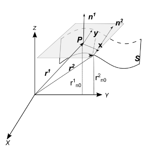
Figure 1: This schematic picture shows the local approximation for the surface $S$ about a point $P$. Points $P$ and $Q$ are localized by vectors $\vec{r}^{\,(1)}$ and $\vec{r}^{\,(2)}$ respectively, and the normal vectors to the surface at those points are $\hat{n}^{(1)}$ and $\hat{n}^{(2)}$. Point $P$ is chosen as the origin of the local coordinate system whereas $Q$ is outside the tangent plane. Its projection onto this tangent plane has coordinates $(x,y)$. The radius of localization of the Gibbs dividing surface is at $r_{n0}^{(1)}$. The distance from $Q$ to the local plane (projection of $\hat{n}^{(2)}$ onto the direction $\hat{n}^{(1)}$) is $r_{n0}^{(1)}-r_{n0}^{(2)}=z$, with $z$ seen from the local system as a paraboloid.

$$z={1\over 2}\left({x^{2}\over R_{1}}+{y^{2}\over R_{2}}\right)+\cdots$$ (26)

As vector $\vec{r}^{\,(2)}$ is not parallel to the $z$ axis of the coordinate system, the normal vector at point $Q$ is given by

$$\hat{n}^{(2)}={\left(-{x\over R_{1}},-{y\over R_{2}},1\right)\over\left[1+({x\over R_{1}})^{2}+({y\over R_{2}})^{2}\right]^{1\over 2}}.$$ (27)

The metric in this coordinate system is $g=1+[\nabla z(x,y)]^{2}=1+{x^{2}\over R^{2}_{1}}+{y^{2}\over R^{2}_{2}}$, where $\frac{x}{R_{1}}\ll 1$ and $\frac{y}{R_{2}}\ll 1$. The surface element in the local system is $dS^{(2)}=g^{1\over 2}dxdy$. The scalar product of the normals is $\hat{n}^{(1)}\cdot\hat{n}^{(2)}=g^{-{1\over 2}}$. We incorporate the effect of the local approximation into the interaction potential to obtain the free energy of the interfacial region

$$\Omega_{S} = -\frac{(\Delta\rho_{0})^{2}}{4}\int dS^{(1)}\int_{-\infty}^{\infty}dx\int_{-\infty}^{\infty}dy\int^{\infty}_{0}dt$$ (28)

$${}\times\tilde{\omega}\left(t+x^{2}+y^{2}+{1\over 4}\left({x^{2}\over R_{1}}+{y^{2}\over R_{2}}\right)^{2}+\cdots\right).$$

By expanding the interaction potential to first order about $t+x^{2}+y^{2}$ and evaluating the integrals on the coordinates $x$ and $y$, one gets to a microscopic expression for the grand potential in terms of the principal radii of curvature

$$\Omega_{S} = -\int dS\left\{{(\Delta\rho_{0})^{2}\pi\over 2}\int_{0}^{\infty}dr\tilde{\omega}(r^{2})r^{3}\right\}$$ (29)

$$+ \int dS\bigg{(}{1\over R_{1}^{2}}+{1\over R_{2}^{2}}+{2\over 3R_{1}R_{2}}\bigg{)}\left\{{3(\Delta\rho_{0})^{2}\pi\over 64}\int_{0}^{\infty}dr\tilde{\omega}(r^{2})r^{5}\right\}+\cdots$$

where we have put $dS^{(1)}=dS$. On the other hand, from the definitions of the mean ($H$) and Gaussian ($K$) curvatures one finds that

$$4H^{2}-{4\over 3}K={1\over R_{1}^{2}}+{1\over R_{2}^{2}}+{2\over 3R_{1}R_{2}}.$$ (30)

By introducing this into (29), we get to the most general microscopic expression for the grand potential within this approximation level; consistent with the Helfrich prediction [13] for the free energy

$$\Omega_{S}=-\int dS\bigg{[}\frac{\pi(\Delta\rho_{0})^{2}}{2}\int^{\infty}_{0}drr^{3}\,\tilde{\omega}(r^{2})-\frac{3\pi(\Delta\rho_{0})^{2}}{64}\left(4H^{2}-{4\over 3}K\right)\int drr^{5}\,\tilde{\omega}(r^{2})\bigg{]}.$$ (31)

which is also in agreement with previous results in the planar [5, 7, 12], spherical [12], and cylindrical [12] geometries, as it is shown in Appendix B.

5 Concluding Remarks

There exist two relevant aspects of this work that are worthwhile remarking. The first one concerns a rigorous proof for a general expression, exact and simple, of the grand potential within a mean field approximation. The second is a first principles derivation of the Helfrich free energy, within this context, from a completely original approach. This, in addition, confirms that the Helfrich scheme is appropriate for the study of curved interfaces. Although the local approximation of a surface as a plane that has been used is appropriate for the description of weakly curved surfaces, we observe that the result for the grand potential representing the free energy of the system is sufficiently general. The microscopic expression obtained is a function of the principal curvatures of the surface, in complete agreement with previous predictions [13, 15]. We also find complete consistency with previous results for the simplest geometries, which were obtained using a different analytic approach [12]. Finally, we point out that within the step function approximation for the density profile, no contribution exists from spontaneous curvature to the free energy. We shall study the problem of an arbitrarily curved interface for a more general density profile in a future publication.

Appendix A Simplifications on the Grand Potential

In this appendix we summarize the main steps to simplify Eq. (17). We start by writing it in the form

$$\Omega_{S}=-\frac{1}{2}\int d\vec{r}\int d\vec{r}\,^{\prime}\rho_{0}(\vec{r})\tilde{w}(|\vec{r}\,^{\prime}|)\hat{n}_{\alpha}(\vec{r}\,)\hat{n}_{\beta}(\vec{r}\,)r_{\beta}^{\prime}{\nabla}_{\alpha}\rho_{0}(\vec{r}+\vec{r}\,^{\prime})+T_{1}+T_{2}+T_{3}+T_{4},$$ (32)

where the $T_{i}$, with $i=1,\ldots,4$, have been defined as the integrals appearing in (17) sequentially.

In order to simplify and easily identify each of the terms $T_{1}$, $T_{2}$, $T_{3}$, and $T_{4}$, we introduce explicitly the change of variables (12)–(13). Under such a coordinate transformation the term $T_{1}$ reads

$$T_{1}=-{1\over 4}\int d\vec{r}^{\,(1)}\int d\vec{r}^{\,(2)}\int_{0}^{1}d\lambda\lambda\int_{0}^{\infty}dt\,\tilde{\omega}(t+|\vec{r}^{\,(2)}|^{2})\partial_{n}^{(1)}\rho_{0}(\vec{r}^{\,(1)}-\vec{r}^{\,(2)})\partial_{n}^{(1)}\rho_{0}(\vec{r}^{\,(1)}),$$ (33)

where the notation $\partial_{n}^{(1)}={\partial}/{\partial r_{n}^{(1)}}$ has been introduced. Integrating by parts with respect to $r^{(1)}_{n}$, this now becomes

$$T_{1}={1\over 4}\int d\vec{r}^{\,(1)}\int d\vec{r}^{\,(2)}\int_{0}^{1}d\lambda\lambda\int_{0}^{\infty}dt\,\tilde{\omega}(t+|\vec{r}^{\,(2)}|^{2})\rho_{0}(\vec{r}^{\,(1)}-\vec{r}^{\,(2)})\partial_{n}^{(1)2}\rho_{0}(\vec{r}^{\,(1)}).$$ (34)

The other term with normal derivatives of the same order is $T_{2}$. The effect of transformation (12)–(13) into this leads to

$$T_{2} = -{1\over 4}\int d\vec{r}^{\,(1)}\int d\vec{r}^{\,(2)}\int_{0}^{1}d\lambda\lambda\int_{0}^{\infty}dt\,\tilde{\omega}(t+|\vec{r}^{\,(2)}|^{2})\rho_{0}(\vec{r}^{\,(1)}-\vec{r}^{\,(2)})\partial_{n}^{(1)2}\rho_{0}(\vec{r}^{\,(1)})$$ (35)

$$= -T_{1}.$$

Therefore these terms cancel one another when substituted into the expression for the grand potential (32).

To simplify the terms with normal derivatives of the second order, that is $T_{3}$ and $T_{4}$, we need to take into account the following manipulations

$${\partial\over\partial r^{\prime}_{n}}={\partial r_{n}^{(1)}\over\partial r^{\prime}_{n}}{\partial\over\partial r_{n}^{(1)}}+{\partial r_{n}^{(2)}\over\partial r^{\prime}_{n}}{\partial\over\partial r_{n}^{(2)}}=\lambda{\partial\over\partial r_{n}^{(1)}}+{\partial\over\partial r_{n}^{(2)}}=\lambda\partial_{n}^{(1)}+\partial_{n}^{(2)},$$ (36)

from where

$${\partial^{2}\over\partial r^{{}^{\prime}2}_{n}} = {\partial\over\partial r^{\prime}_{n}}\left(\lambda\partial_{n}^{(1)}+\partial_{n}^{(2)}\right)=\lambda^{2}\partial_{n}^{(1)2}+2\lambda\partial_{n}^{(1)}\partial_{n}^{(2)}+\partial_{n}^{(2)2}.$$ (37)

By introducing this into $T_{3}$, we obtain

$$T_{3} = -{1\over 8}\int d\vec{r}^{\,(1)}\int d\vec{r}^{\,(2)}\int_{0}^{1}d\lambda\lambda\int_{0}^{\infty}dt\int_{0}^{\infty}dt^{\prime}\tilde{\omega}(t+t^{\prime}+|\vec{r}^{\,(2)}|^{2})$$ (38)

$$\times \left[\lambda^{2}\partial_{n}^{(1)2}+2\lambda\partial_{n}^{(1)}\partial_{n}^{(2)}+\partial_{n}^{(2)2}\right]\left[\partial_{n}^{(1)}\rho_{0}(\vec{r}^{\,(1)}-\vec{r}^{\,(2)})\partial_{n}^{(1)}\rho_{0}(\vec{r}^{\,(1)})\right].$$

We need to calculate derivatives of the product within the integrand. The first one is

$$\partial_{n}^{(1)}[\partial_{n}^{(1)}\rho_{0}(\vec{r}^{\,(1)}-\vec{r}^{\,(2)})\partial_{n}^{(1)}\rho_{0}(\vec{r}^{\,(1)})] = \partial_{n}^{(1)2}\rho_{0}(\vec{r}^{\,(1)}-\vec{r}^{\,(2)})\partial_{n}^{(1)}\rho_{0}(\vec{r}^{\,(1)})$$ (39)

$$+ \partial_{n}^{(1)}\rho_{0}(\vec{r}^{\,(1)}-\vec{r}^{\,(2)})\partial_{n}^{(1)2}\rho_{0}(\vec{r}^{\,(1)}),$$

and the second

$$\partial_{n}^{(1)2}[\partial_{n}^{(1)}\rho_{0}(\vec{r}^{\,(1)}-\vec{r}^{\,(2)})\partial_{n}^{(1)}\rho_{0}(\vec{r}^{\,(1)})] = \partial_{n}^{(1)}[\partial_{n}^{(1)2}\rho_{0}(\vec{r}^{\,(1)}-\vec{r}^{\,(2)})\partial_{n}^{(1)}\rho_{0}(\vec{r}^{\,(1)})$$ (40)

$$+ \partial_{n}^{(1)}\rho_{0}(\vec{r}^{\,(1)}-\vec{r}^{\,(2)})\partial_{n}^{(1)2}\rho_{0}(\vec{r}^{\,(1)})]$$

$$= \partial_{n}^{(1)3}\rho_{0}(\vec{r}^{\,(1)}-\vec{r}^{\,(2)})\partial_{n}^{(1)}\rho_{0}(\vec{r}^{\,(1)})$$

$$+ 2\partial_{n}^{(1)2}\rho_{0}(\vec{r}^{\,(1)}-\vec{r}^{\,(2)})\partial_{n}^{(1)2}\rho_{0}(\vec{r}^{\,(1)})$$

$$+ \partial_{n}^{(1)}\rho_{0}(\vec{r}^{\,(1)}-\vec{r}^{\,(2)})\partial_{n}^{(1)3}\rho_{0}(\vec{r}^{\,(1)}).$$

The corresponding derivatives for $\partial_{n}^{(2)}$ are also calculated. By introducing all these into $T_{3}$ one finds

$$T_{3} = -{1\over 8}\int d\vec{r}^{\,(1)}\int d\vec{r}^{\,(2)}\int_{0}^{1}d\lambda\lambda\int_{0}^{\infty}dt\int_{0}^{\infty}dt^{\prime}\tilde{\omega}(t+t^{\prime}+|\vec{r}^{\,(2)}|^{2})$$

$$\times \{\lambda^{2}[\partial_{n}^{(1)3}\rho_{0}(\vec{r}^{\,(1)}-\vec{r}^{\,(2)})\partial_{n}^{(1)}\rho_{0}(\vec{r}^{\,(1)})+\partial_{n}^{(1)2}\rho_{0}(\vec{r}^{\,(1)}-\vec{r}^{\,(2)})\partial_{n}^{(1)2}\rho_{0}(\vec{r}^{\,(1)})$$

$$+ \partial_{n}^{(1)}\rho_{0}(\vec{r}^{\,(1)}-\vec{r}^{\,(2)})\partial_{n}^{(1)3}\rho_{0}(\vec{r}^{\,(1)})]+2\lambda[\partial_{n}^{(1)2}\rho_{0}(\vec{r}^{\,(1)}-\vec{r}^{\,(2)})\partial_{n}^{(1)}\rho_{0}(\vec{r}^{\,(1)})$$

$$+ \partial_{n}^{(1)}\rho_{0}(\vec{r}^{\,(1)}-\vec{r}^{\,(2)})\partial_{n}^{(1)2}\rho_{0}(\vec{r}^{\,(1)})]+\partial_{n}^{(2)2}[\partial_{n}^{(1)}\rho_{0}(\vec{r}^{\,(1)}-\vec{r}^{\,(2)})\partial_{n}^{(1)}\rho_{0}(\vec{r}^{\,(1)})]\}.$$

or alternatively, after an integration by parts respect to $r_{n}^{(1)}$ in each term,

$$T_{3} = {1\over 8}\int d\vec{r}^{\,(1)}\int d\vec{r}^{\,(2)}\int_{0}^{1}d\lambda\lambda\int_{0}^{\infty}dt\int_{0}^{\infty}dt^{\prime}\tilde{\omega}(t+t^{\prime}+|\vec{r}^{\,(2)}|^{2})$$ (42)

$$\times \{\lambda^{2}[\partial_{n}^{(1)2}\rho_{0}(\vec{r}^{\,(1)}-\vec{r}^{\,(2)})\partial_{n}^{(1)2}\rho_{0}(\vec{r}^{\,(1)})2\partial_{n}^{(1)}\rho_{0}(\vec{r}^{\,(1)}-\vec{r}^{\,(2)})\partial_{n}^{(1)3}\rho_{0}(\vec{r}^{\,(1)})$$

$$+ \rho_{0}(\vec{r}^{\,(1)}-\vec{r}^{\,(2)})\partial_{n}^{(1)4}\rho_{0}(\vec{r}^{\,(1)}]+2\lambda\partial_{n}^{(2)}[\partial_{n}^{(1)}\rho_{0}(\vec{r}^{\,(1)}-\vec{r}^{\,(2)})\partial_{n}^{(1)2}\rho_{0}(\vec{r}^{\,(1)})$$

$$+ \rho_{0}(\vec{r}^{\,(1)}-\vec{r}^{\,(2)})\partial_{n}^{(1)3}\rho_{0}(\vec{r}^{\,(1)})]+\partial_{n}^{(2)2}[\rho_{0}(\vec{r}^{\,(1)}-\vec{r}^{\,(2)})\partial_{n}^{(1)2}\rho_{0}(\vec{r}^{\,(1)})]\}.$$

Now we investigate the effect of the same transformation in the expression for $T_{4}$. Direct substitution implies

$$T_{4} = -{1\over 8}\int d\vec{r}^{\,(1)}\int d\vec{r}^{\,(2)}\int_{0}^{1}d\lambda\lambda\int_{0}^{\infty}dt\int_{0}^{\infty}dt^{\prime}\tilde{\omega}(t+t^{\prime}+|\vec{r}^{\,(2)}|^{2})$$ (43)

$$\times \left[\lambda^{2}\partial_{n}^{(1)2}+2\lambda\partial_{n}^{(1)}\partial_{n}^{(2)}+\partial_{n}^{(2)2}\right]\left[\rho_{0}(\vec{r}^{\,(1)}-\vec{r}^{\,(2)})\partial_{n}^{(1)2}\rho_{0}(\vec{r}^{\,(1)})\right].$$

Although this compact form appears simple, we need to carry out further simplifications to identify similar terms. We start by calculating the first derivative

$$\partial_{n}^{(1)}[\rho_{0}(\vec{r}^{\,(1)}-\vec{r}^{\,(2)})\partial^{(1)2}\rho_{0}(\vec{r}^{\,(1)})] = \partial_{n}^{(1)}\rho_{0}(\vec{r}^{\,(1)}-\vec{r}^{\,(2)})\partial_{n}^{(1)2}\rho_{0}(\vec{r}^{\,(1)})$$ (44)

$$+ \rho_{0}(\vec{r}^{\,(1)}-\vec{r}^{\,(2)})\partial_{n}^{(1)3}\rho_{0}(\vec{r}^{\,(1)}).$$

and then a further derivative of this quantity in the same direction $\partial_{n}^{(1)}$, which yields

$$\partial_{n}^{(1)2}[\rho_{0}(\vec{r}^{\,(1)}-\vec{r}^{\,(2)})\partial_{n}^{(1)2}\rho_{0}(\vec{r}^{\,(1)})] = \partial_{n}^{(1)}[\partial_{n}^{(1)}\rho_{0}(\vec{r}^{\,(1)}-\vec{r}^{\,(2)})\partial_{n}^{(1)2}\rho_{0}(\vec{r}^{\,(1)})$$ (45)

$$+ \rho_{0}(\vec{r}^{\,(1)}-\vec{r}^{\,(2)})\partial_{n}^{(1)3}\rho_{0}(\vec{r}^{\,(1)})]$$

$$= \partial_{n}^{(1)2}\rho_{0}(\vec{r}^{\,(1)}-\vec{r}^{\,(2)})\partial_{n}^{(1)2}\rho_{0}(\vec{r}^{\,(1)})$$

$$+ 2\partial_{n}^{(1)}\rho_{0}(\vec{r}^{\,(1)}-\vec{r}^{\,(2)})\partial_{n}^{(1)3}\rho_{0}(\vec{r}^{\,(1)})$$

$$+ \rho_{0}(\vec{r}^{\,(1)}-\vec{r}^{\,(2)})\partial_{n}^{(1)4}\rho_{0}(\vec{r}^{\,(1)}).$$

By substituting we find

$$T_{4} = -{1\over 8}\int d\vec{r}^{\,(1)}\int d\vec{r}^{\,(2)}\int_{0}^{1}d\lambda\lambda\int_{0}^{\infty}dt\int_{0}^{\infty}dt^{\prime}\tilde{\omega}(t+t^{\prime}+|\vec{r}^{\,(2)}|^{2})$$ (46)

$$\times \{\lambda^{2}[\partial_{n}^{(1)2}\rho_{0}(\vec{r}^{\,(1)}-\vec{r}^{\,(2)})\partial_{n}^{(1)2}\rho_{0}(\vec{r}^{\,(1)})+2\partial_{n}^{(1)}\rho_{0}(\vec{r}^{\,(1)}-\vec{r}^{\,(2)})\partial_{n}^{(1)3}\rho_{0}(\vec{r}^{\,(1)})$$

$$+ \rho_{0}(\vec{r}^{\,(1)}-\vec{r}^{\,(2)})\partial_{n}^{(1)4}\rho_{0}(\vec{r}^{\,(1)})]+2\lambda\partial_{n}^{(2)}[\partial_{n}^{(1)}\rho_{0}(\vec{r}^{\,(1)}-\vec{r}^{\,(2)})\partial_{n}^{(1)2}\rho_{0}(\vec{r}^{\,(1)})$$

$$+ \rho_{0}(\vec{r}^{\,(1)}-\vec{r}^{\,(2)})\partial_{n}^{(1)3}\rho_{0}(\vec{r}^{\,(1)})]+\partial_{n}^{(2)2}[\rho_{0}(\vec{r}^{\,(1)}-\vec{r}^{\,(2)})\partial_{n}^{(1)2}\rho_{0}(\vec{r}^{\,(1)})]\}$$

$$= -T_{3}.$$

That is, also the terms $T_{3}$ and $T_{4}$ cancel one another.

Appendix B Simplest Geometries

To make contact with previous results we consider here the simplest geometries. For the planar surface $R_{1}=R_{2}=\infty$ so that $4H^{2}-{4\over 3}K=0$ and thus Eq. (31) simplifies to

$$\Omega_{S}=-\int dS\bigg{[}\frac{\pi(\Delta\rho_{0})^{2}}{2}\int^{\infty}_{0}drr^{3}\,\tilde{\omega}(r^{2})\bigg{]}.$$ (47)

That is, the only contribution to the free energy comes from the surface tension term, in agreement with previous results [5, 7, 12].

For a spherical interface $R_{1}=R_{2}=R$, $H={1\over R}$, and $K={1\over R^{2}}$, so that $4H^{2}-{4\over 3}K={8\over 3R^{2}}$. From (31) one gets to the corresponding free energy

$$\Omega_{S}=-\int dS\bigg{[}\frac{\pi(\Delta\rho_{0})^{2}}{2}\int^{\infty}_{0}drr^{3}\,\tilde{\omega}(r^{2})-\frac{\pi(\Delta\rho_{0})^{2}}{8R^{2}}\int drr^{5}\,\tilde{\omega}(r^{2})\bigg{]}.$$ (48)

Finally, for the cylindrical interface $R_{1}=\infty$ and $R_{2}=R$, so that $4H^{2}-{4\over 3}K={1\over R^{2}}$. In this case the free energy is

$$\Omega_{S}=-\int dS\bigg{[}\frac{\pi(\Delta\rho_{0})^{2}}{2}\int^{\infty}_{0}drr^{3}\,\tilde{\omega}(r^{2})-\frac{3\pi(\Delta\rho_{0})^{2}}{64R^{2}}\int drr^{5}\,\tilde{\omega}(r^{2})\bigg{]}.$$ (49)

These last two expressions are consistent with previous results [12].

References

• [1] R. Evans, Adv. Phys. 28, 143 (1979).
• [2] J. S. Rowlinson and B. Widom, Molecular Theory of Capillarity (Clarendon, Oxford, 1982).
• [3] R. C. Tolman, J. Chem. Phys. 17, 333 (1949).
• [4] S. Dietrich and M. Napiorkowski, Physica A 177, 437 (1991);
M. Napiorkowski and S. Dietrich, Phys. Rev. E 47, 1836 (1993);
M. Napiorkowski and S. Dietrich, Z. Phys. B 97, 511 (1995);
K. R. Mecke and S. Dietrich, Phys. Rev. E 59, 6766 (1999);
K. R. Mecke and S. Dietrich, J. Chem. Phys. 123, 204723 (2005).
• [5] D. G. Triezenberg and R. Zwanzig, Phys. Rev. Lett. 28, 1183 (1972). This result is known to have been obtained by Yvon but he did not published it.
• [6] A. J. M. Yang, P. D. Fleming, and J. H. Gibbs, J. Chem. Phys. 64, 3732 (1976);
A. J. M. Yang, P. D. Fleming, and J. H. Gibbs, J. Chem. Phys. 67, 74 (1977).
• [7] E. M. Blokhuis and D. Bedeaux, Physica A 184, 42 (1992);
E. M. Blokhuis and D. Bedeaux, Mol. Phys. 80, 705 (1993);
A. E. van Giessen, E. M. Blokhuis, and D. J. Bukman, J. Chem. Phys. 108, 1148 (1998).
• [8] J. K. Percus, in The Liquid State of Matter: Fluids, Simple and Complex, E. W. Montroll and J. L. Lebowitz, eds. (North-Holland, Amsterdam, 1982).
• [9] V. Romero-Rochín, C. Varea, and A. Robledo Phys. Rev. A 44, 8417, (1991);
V. Romero-Rochín, C. Varea, and A. Robledo, Physica A 184, 367 (1992);
V. Romero-Rochín, C. Varea, and A. Robledo, Mol. Phys. 80, 821 (1993);
V. Romero-Rochín, C. Varea, and A. Robledo, Phys. Rev. E 48, 1600 (1993).
• [10] J. K. Percus, J. Math. Phys. 37, 1259 (1996).
• [11] V. Romero-Rochín and J. K. Percus, Phys. Rev. E 53, 5130 (1996).
• [12] Jóse G. Segovia-López and Víctor Romero-Rochín, Phys. Rev. E 73, 021601, (2006).
• [13] W. Helfrich, Z. Naturfosch. Teil A 28, 693 (1973).
• [14] C. Varea and A. Robledo, Physica A 220, 33 (1995);
C. Varea and A. Robledo, Mol. Phys. 85, 477 (1995).
• [15] A. Robledo and C. Varea, Physica A 231, 178 (1996).
• [16] L. D. Landau and E. M. Lifshitz, Theory of Elasticity (Pergamon Press, Oxford, 1984).
• [17] R. Balian and C. Bloch, Ann. Phys. (N. Y.) 60, 401 (1970).
• [18] Bertand Duplantier, Raymond E. Goldstein, Victor Romero-Rochín, and Adriana I. Pesci, Phys. Rev. Lett. 65, 508 (1990).