Laplace deconvolution with noisy observations

Abstract

In the present paper we consider Laplace deconvolution problem for discrete noisy data observed on an interval whose length $T_{n}$ may increase with the sample size. Although this problem arises in a variety of applications, to the best of our knowledge, it has been given very little attention by the statistical community. Our objective is to fill the gap and provide statistical analysis of Laplace deconvolution problem with noisy discrete data. The main contribution of the paper is explicit construction of an asymptotically rate-optimal (in the minimax sense) Laplace deconvolution estimator which is adaptive to the regularity of the unknown function. We show that the original Laplace deconvolution problem can be reduced to nonparametric estimation of a regression function and its derivatives on the interval of growing length $T_{n}$. Whereas the forms of the estimators remains standard, the choices of the parameters and the minimax convergence rates, which are expressed in terms of $T_{n}^{2}/n$ in this case, are affected by the asymptotic growth of the length of the interval.

We derive an adaptive kernel estimator of the function of interest, and establish its asymptotic minimaxity over a range of Sobolev classes. We illustrate the theory by examples of construction of explicit expressions of Laplace deconvolution estimators. A simulation study shows that, in addition to providing asymptotic optimality as the number of observations tends to infinity, the proposed estimator demonstrates good performance in finite sample examples.

AMS 2010 subject classifications. 62G05, 62G20.
Key words and phrases: adaptivity, kernel estimation, minimax rates, Volterra equation, Laplace convolution

1 Introduction

1.1 Formulation and motivation

Mathematical modeling of a variety of problems in population dynamics, mathematical physics, theory of superfluidity and many others fields leads to the convolution type Volterra equation of the first kind of the form

$$q(t)=\int_{0}^{t}g(t-\tau)f(\tau)d\tau,\quad t\geq 0,$$ (1.1)

where $q(t)$ is the known or observed function, $g(t)$ is the known kernel and $f(t)$ is the unknown function to be solved for.

Note that the LHS of equation (1.1) is well defined for any $t\geq 0$ if functions $f$ and $g$ are Riemann integrable on any finite sub-interval of $[0,\infty)$. In particular, $f$ and $g$ do not need to be absolutely or square integrable on the nonnegative half-line. Assume the existence of their Laplace transforms $\tilde{f}(s)$ and $\tilde{g}(s)$ for all $s\geq 0$, where

$$\tilde{f}(s)=\int_{0}^{\infty}e^{-sx}f(x)dx,\quad{\rm and}\quad\tilde{g}(s)=\int_{0}^{\infty}e^{-sx}g(x)dx,\quad s\geq 0.$$ (1.2)

In the Laplace domain, equation (1.1) becomes $\tilde{q}(s)=\tilde{g}(s)\tilde{f}(s)$ and, therefore, the problem (1.1) is also known as Laplace deconvolution problem.

In practice, however, one typically has only discrete observations of the function $q$ in (1.1) which are available only on a finite interval and, in addition, are corrupted by noise, that leads to the following discrete noisy version of equation (1.1)

$$y(t_{i})=\int_{0}^{t_{i}}g(t_{i}-\tau)f(\tau)d\tau+\sigma\epsilon_{i},\;\;\;i=1,...,n,$$ (1.3)

where $0\leq t_{1}\leq...\leq t_{n}\leq T_{n}$, $\epsilon_{i}$ are i.i.d. $N(0,1)$ variates, $\sigma$ is the known constant variance and $T_{n}$ may grow with $n$.

Equations of the form (1.3) appear in many practical applications. Investigations in this paper have been motivated by analysis of dynamic contrast enhanced imaging data and modeling of time-resolved measurements in fluorescence spectroscopy.

Example 1.

Dynamic contrast enhanced imaging data (DCE-imaging). DCE-imaging is widely used in cancer research (see, e.g., Cao et al., 2010; Goh et al., 2005; Goh and Padhani, 2007; Cuenod et al., 2006; Cuenod et al., 2011; Miles, 2003; Padhani and Harvey, 2005 and Bisdas et al., 2007). Such imaging procedures have great potential for tumor detection and characterization, as well as for monitoring in vivo the effects of treatments. DCE-imaging follows the diffusion of a bolus of a contrast agent injected into a vein. At the microscopic level, for a given unit volume voxel of interest, denote by $Y(t)$ the number of particles in the voxel at time $t$ and by $F(t)$ the c.d.f. of a random lapse of time during which a particle sojourns in the voxel of interest. Then, $F(t)$ satisfies the following equation which can be viewed as a particular case of equation (1.3):

$$Y(t_{i})=\int_{0}^{t_{i}}AIF(t-\tau)(1-F(\tau))d\tau+\sigma\epsilon_{i},$$ (1.4)

where $AIF(t)$ is the Arterial Input Function which measures concentration of particles within a unit volume voxel inside a large artery and can be estimated relatively easily. Physicians are interested in a reproducible quantification of the blood flow inside the tissue which is characterized by $f(t)=1-F(t)$, since this quantity is independent of the number of particles of contrast agent injected into the vein.

Example 2.

Time-resolved measurements in fluorescence spectroscopy. Time-resolved measurements in fluorescence spectroscopy are widely used for studies of biological macromolecules and for cellular imaging (see, e.g., Ameloot and Hendrickx, 1983; Ameloot et al., 1984; Gafni, Modlin and Brand, 1975; McKinnon, Szabo and Miller, 1977; O’Connor, Ware and Andre, 1979, and also the monograph of Lakowicz, 2006 and references therein). At present, in fluorescence spectroscopy, most of the time-domain measurements are carried out using time-correlated single-photon counting. The measured intensity decay is represented by the number of photons $N(t_{k})$ that were detected within the time interval $(t_{k},t_{k}+\Delta t)$, and appears as a noisy convolution of the impulse response function $I(t)$ with a known lamp function $L(t)$

$$N(t_{k})=\int_{0}^{t_{k}}L(t_{k}-\tau)I(\tau)d\tau+\sigma\epsilon_{k}.$$

The objective is to determine the impulse response function $I(x)$ that best matches the experimental data.

1.2 Difficulty of the problem

The mathematical theory of (noiseless) convolution type Volterra equations is well developed (see, e.g., Gripenberg, Londen and Staffans, 1990) and the exact solution of (1.1) can be obtained through Laplace transform. However, direct application of Laplace transform for discrete measurements faces serious conceptual and numerical problems. The inverse Laplace transform is usually found by application of tables of inverse Laplace transforms, partial fraction decomposition or series expansion (see, e.g., Polyanin and Manzhirov, 1998), neither of which is applicable in the case of the discrete noisy version of Laplace deconvolution.

Formally, by extending $g(t)$ and $f(t)$ to the negative values of $t$ by setting $f(t)=g(t)=0$ for $t<0$, equation (1.1) can be viewed as a particular case of the Fredholm convolution equation

$$h(t)=\int_{-\infty}^{\infty}g(t-\tau)f(\tau)d\tau,$$ (1.5)

whose discrete stochastic version

$$y(t_{i})=\int_{-\infty}^{\infty}g(t_{i}-\tau)f(\tau)d\tau+\sigma\epsilon_{i},\;\;\;\;i=1,...,n,$$ (1.6)

known also as Fourier deconvolution problem, has been extensively studied in the last thirty years (see, for example, Carroll and Hall, 1988; Comte, Rozenholc and Taupin, 2006, 2007; Delaigle, Hall and Meister, 2008; Diggle and Hall, 1993; Fan, 1991; Fan and Koo, 2002; Johnstone et al., 2004; Pensky and Vidakovic, 1999; Stefanski and Carrol, 1990 among others; see also monograph by Meister,2009 and references therein).

Unfortunately, the existing approaches to Fourier deconvolution cannot be easily extended to solution of noisy discrete version of Laplace convolution equation (1.3). The body of work cited above addresses one of three situations: the case when functions $f$ and $g$ are periodic with period $T$, density deconvolution, and the case of random design, where $t_{i}$ in (1.6) are random variables generated by some density function.

In the first setup, convolution (1.5) becomes circular convolution and measurements in equation (1.6) are taken on an interval of fixed length $T$, so that the problem can be solved by application of discrete Fourier transform. However, since the functions $f$ and $g$ are not periodic on $[0,T_{n}]$, the integral in the RHS of equation (1.3) is not a circular convolution and the discrete Fourier transform cannot be directly applied. Furthermore, the length of the interval $T_{n}$ may grow with $n$ that affects the convergence rates. For relatively small $T_{n}$ (e.g., $T_{n}\sim\log n$), approximation of Fourier transform by its discrete version will be very poor which results in low convergence rates of the estimator of $f$.

Density deconvolution problem and nonparametric regression estimation with random measurements $t_{i}$ typically assume that, as $n\to\infty$, the measurements $t_{i}$ in (1.6) adequately represent the domain of $h(t)$ in (1.5). In these setups observations are absent on a particular part of the domain only if the density which generates those observations is very low. This, however, is not at all true for equation (1.3) where lack of observations for $t>T_{n}$ is due entirely to experimental design and has no relation to the values of the estimated function.

To the best of our knowledge, nobody tackled the problem of Fourier deconvolution (1.6) when observations $t_{i}$ are non-random fixed quantities on an interval of length $T_{n}$ which grows with the number of observations. In addition, we should also mention the important causality property of the Laplace deconvolution not shared by its Fourier counterpart, where the values of $q(t)$ for $0\leq t\leq T_{n}$ depend on values of $f(t)$ for $0\leq t\leq T_{n}$ only and vice versa. Finally, we show that under mild conditions, the solution of the equation (1.3) can be represented explicitly via derivatives of the RHS $q(t)$ that implies computational advantages of the proposed approach.

1.3 Existing results

Only few applied mathematicians took an effort to tackle the problem with discrete measurements in the LHS of (1.1). Ameloot and Hendrickx (1983) applied Laplace deconvolution for the analysis of fluorescence curves and used a parametric presentation of the solution $f$ as a sum of exponential functions with parameters evaluated by minimizing discrepancy with the RHS. In a somewhat similar manner, Maleknejad et al. (2007) proposed to expand the unknown solution over a wavelet basis and find the coefficients via the least squares algorithm. Lien et al. (2008), following Weeks (1966), studied numerical inversion of the Laplace transform using Laguerre functions. Finally, Lamm (1996) and Cinzori and Lamm (2000) used discretization of the equation (1.1) and applied various versions of the Tikhonov regularization technique. However, in all of the above papers, the noise in the measurements was either ignored or treated as deterministic. The presence of random noise in (1.3) makes the problem even more challenging.

Unlike Fourier deconvolution that has been intensively studied in statistical literature (see references above), Laplace deconvolution received virtually no attention within statistical framework. To the best of our knowledge, the only paper which tackles the problem is Dey, Martin and Ruymgaart (1998) which considers a noisy version of Laplace deconvolution with a very specific kernel of the form $g(t)=be^{-at}$. The authors use the fact that, in this case, the solution of the equation (1.1) satisfies a particular linear differential equation and, hence, can be recovered using $q(t)$ and its derivative $q^{\prime}(t)$. For this particular kind of kernel, the authors derived convergence rates for the quadratic risk of the proposed estimators, as $n$ increases, under the assumption that the $m$-th derivative of $f$ is continuous on $(0,\infty)$. However, they assume that data is available on the whole nonnegative half-line (i.e. $T_{n}=\infty$) and that $m$ is known (i.e., the estimator is not adaptive).

1.4 Objectives and organization of the paper

For the reasons listed above, estimation of $f$ from discrete noisy observations $y$ in (1.3) requires development of a novel approach. The objective of the present paper is to fill the gap and to develop general statistical methodology for Laplace deconvolution problem which allows to circumvent lack of observations for $t>T_{n}$ and leads to effective representation of $f$ on the interval $(0,T_{n})$, no matter what value $T_{n}$ takes. We establish minimax convergence rates for Laplace deconvolution setup over Sobolev classes and derive the adaptive estimator of $f$ which is rate-optimal over entire range of Sobolev classes. The proposed estimator is based on estimating $q$ and its derivatives from noisy data $y$ in (1.3), where $q(t)=(f\ast g)(t)=\int_{0}^{t}g(t-\tau)f(\tau)d\tau$ is the convolution of $f$ and $g$. Thus, one can use the numerous existing techniques for nonparametric estimation of a function and its derivatives. In particular, we employ kernel estimators with the global bandwidth adaptively selected by Lepski procedure.

An attractive feature of the estimation technique proposed in this paper is that estimator of $f$ is expressed explicitly via $q$ and its derivatives. Another interesting aspect of the considered model (1.3) is that the data is observed on the interval of asymptotically increasing length, where $T_{n}\rightarrow\infty$ as $n\rightarrow\infty$. This is indeed a reasonable assumption since, as $n$ is growing, demands on the improvements of the estimation precision require to decrease the bias by sampling $q(t)$ for larger and larger values of $t$. Dependence of $T$ on $n$ may not significantly affect estimation procedures but evidently leads to different convergence rates that are formulated in terms of $T_{n}^{2}/n$.

The rest of the paper is organized as follows. Section 2 delivers main results of the paper. In particular, Section 2.1 introduces notations and assumptions used throughout the paper. In Section 2.2 we derive the lower bounds on the minimax risk of estimating $f$ in (1.3). Section 2.3 reviews some mathematical results for noiseless Laplace deconvolution relevant for constructing the proposed estimator. Section 2.4 is dedicated to explicit derivation of Laplace deconvolution estimator in model (1.3), while Section 2.5 establishes its asymptotic adaptive minimaxity over entire range of Sobolev classes. Section 3.1 contains examples of explicit estimators of Laplace deconvolution for various types of kernels $g$. The results of a simulation study are presented in Section 3.2. Section 4 concludes the paper with discussion. All the proofs are given in Appendix.

2 Main results

2.1 Notations and assumptions

In this section we introduce notations and assumptions used throughout the paper.

The $L_{k}(\mathbb{R}^{+})$-norm of the function $h$ is denoted by $\|h\|_{k}$ and $\|h\|_{\infty}$ is the supremum norm of $h$. If $k=2$ and there is no ambiguity, we shall omit the subscript in the notation of the norm, i.e. $\|h\|=\|h\|_{2}$. We use the standard notation $W^{r,p}(\mathbb{R}^{+})$ for a Sobolev space of functions on $[0,\infty)$ that have $r$ weak derivatives with finite $L_{p}$-norms and omit $p$ in this notation if $p=2$, that is, $W^{r}(\mathbb{R}^{+})=W^{r,2}(\mathbb{R}^{+})$. In addition, we shall omit $\mathbb{R}^{+}$ in the notations of the norms and functional spaces and, unless the opposite is stated, assume that all functions are defined on the nonnegative part of the real line.

Let $r\geq 1$ be such that

$$g^{(j)}(0)=\left\{\begin{array}[]{ll}0,&\mbox{if}\ \ j=0,...,r-2,\\ B_{r}\neq 0,&\mbox{if}\ \ j=r-1,\end{array}\right.$$ (2.1)

with obvious modification $g(0)=B_{1}\neq 0$ for $r=1$.

Assume now the following conditions on the unknown $f$ and the known kernel $g$ in (1.1):

• $g\in W^{r,1}\cap W^{\nu}$, $\nu\geq r$.

• Let $\Omega$ be a collection of distinct zeros $s_{\omega}$ of the Laplace transform $\tilde{g}$ of $g$. Then all zeros of $\tilde{g}$ have negative real parts, i.e.,

  $$s^{*}=\max_{s_{\omega}\in\Omega}Re(s_{\omega})<0.$$

• $f\in W^{m}$ where $m\leq\nu+1-r$.

Finally, we impose the following assumption on $T_{n}$ and design points $t_{i}$, $i=1,...,n$:

• Let $T_{n}$ be such that $T_{n}\rightarrow\infty$ but $n^{-1}\,T_{n}^{2}\rightarrow 0$ as $n\rightarrow\infty$ and there exist $1\leq\mu<\infty$ such that $\max_{i}\,|t_{i}-t_{i-1}|\leq\mu n^{-1}T_{n}$.

In what follows, we use the symbol $C$ for a generic positive constant, independent of the sample size $n$, which may take different values at different places.

2.2 Lower bounds for the minimax risk

In order to establish a benchmark for an estimator of an unknown function $f$ from its noisy Laplace convolution (1.3) we derive the asymptotic minimax lower bounds for the $L_{2}([0,T_{n}])$-risk over a Sobolev ball $W^{m}(A)$ of radius $A$. It turns out that, unlike in the density deconvolution problem or Fourier deconvolution setup, the rates of convergence depend on the length of the interval $T_{n}$ and are expressed in terms of the ratio $T_{n}^{2}/n$:

Theorem 1.

Let condition (2.1) and Assumptions (A1)–(A4) hold. Then, there exists a constant $C>0$ such that

$$\inf_{\hat{f}_{n}}\sup_{f\in W^{m}(A)}E||\hat{f}_{n}-f||^{2}_{L_{2}([0,T_{n}])}\geq C\left(\frac{T_{n}^{2}}{n}\right)^{\frac{2m}{2(m+r)+1}},$$ (2.2)

where the infimum is taken over all possible estimators $\hat{f}_{n}$ of $f$, and, therefore,

$$\inf_{\hat{f}_{n}}\sup_{f\in W^{m}(A)}E||\hat{f}_{n}-f||^{2}_{L_{2}([0,\infty))}\geq C\left(\frac{T_{n}^{2}}{n}\right)^{\frac{2m}{2(m+r)+1}}.$$

2.3 Solution of noiseless Volterra equation

As we have already mentioned, unlike Fourier deconvolution, an estimator $\hat{f}_{n}$ of the unknown $f$ in (1.3) can be obtained explicitly in the closed form. To understand the motivation for the proposed $\hat{f}_{n}$ we find first the exact solution of the noiseless Volterra equation (1.1).

Taking derivatives of both sides of (1.1) under (2.1) and Assumptions (A1), (A3), one obtains

$$q^{(j)}(t) = \int_{0}^{t}g^{(j)}(t-\tau)f(\tau)d\tau,\ \ j=1,...,r-1;$$

$$\cdot \cdot \cdot$$

$$q^{(r)}(t) = B_{r}f(t)+\int_{0}^{t}g^{(r)}(t-\tau)f(\tau)d\tau,$$ (2.3)

which is the Volterra equation of the second kind. Taking higher-order derivatives, (2.3) yields

$$q^{(r+1)}(t) = B_{r}f^{\prime}(t)+g^{(r)}(t)f(0)+\int_{0}^{t}g^{(r)}(t-\tau)f^{\prime}(\tau)d\tau,$$

$$\cdot \cdot \cdot$$

$$q^{(r+m)}(t) = B_{r}f^{(m)}(t)+\sum_{j=0}^{m-1}g^{(r+j)}(t)f^{(j)}(0)+\int_{0}^{t}g^{(r)}(t-\tau)f^{(m)}(\tau)d\tau.$$

Then, under Assumptions (A1) and (A3), one has $q^{(r+m)}\in L_{2}$ and, hence, $q\in W^{r+m}$.

In addition, due to Assumptions (A1) and (A3), condition (2.3) implies that $q^{(r)}\in L_{1}$ and, therefore, one can use the following known facts from the theory of Volterra equations of the second kind:

1. there exists a unique solution $\phi$ of the equation

   $$g^{(r)}(t)=B_{r}\phi(t)+\int_{0}^{t}g^{(r)}(t-\tau)\phi(\tau)d\tau$$ (2.4)

   called a resolvent of $g^{(r)}$ (see Theorem 3.1 of Gripenberg, Londen and Staffans, 1990);

2. there exists a unique solution $f$ of (2.3) and, therefore, of the original equation (1.1), which can be written as

   $$f(t)=B_{r}^{-1}q^{(r)}(t)-B_{r}^{-1}\int_{0}^{t}q^{(r)}(t-\tau)\phi(\tau)d\tau$$ (2.5)

   (see Theorem 3.5 of Gripenberg, Londen and Staffans, 1990).

Remark 1.

Assumption (A2) ensures that the solution $f(t)$ of the noiseless Laplace convolution equation (1.1) is numerically stable. By Half-Line Paley-Wiener theorem (see Theorem 2.4.1 of Gripenberg, Londen and Staffans, 1990), the resolvent $\phi(\tau)$ of $g$ in (2.4) is absolutely integrable if and only if Assumption (A2) is satisfied. If $\tilde{g}$ has roots with positive real parts, then, by Corollary 2.4.2 from the same book, $\phi(\tau)$ is growing at an exponential rate, so that $e^{-s\tau}\phi(\tau)$ is absolutely integrable for any $s>s^{*}$, where $s^{*}$ is defined in assumption (A2).

It follows from the above that, in order to solve the noiseless Volterra equation (1.1), one only needs to determine a resolvent $\phi$ in (2.4) defined entirely by the $r$-th derivative $g^{(r)}$ of the (known) kernel $g$. Taking Laplace transform of both sides of (2.4) yields

$$\widetilde{g^{(r)}}(s)=B_{r}\tilde{\phi}(s)+\widetilde{g^{(r)}}(s)\tilde{\phi}(s)$$

where, due to (2.1), one has $\widetilde{g^{(r)}}(s)=s^{r}\tilde{g}(s)-B_{r}$. Therefore, $\phi(t)$ can be obtained as an inverse Laplace transform of $\tilde{\phi}$, where

$$\tilde{\phi}(s)=\frac{s^{r}\tilde{g}(s)-B_{r}}{s^{r}\tilde{g}(s)}.$$ (2.6)

Behavior of the resolvent function $\phi$ is thus determined by the properties $\tilde{g}$. It turns out (see, e.g., Gripenberg, Londen and Steffans 1990, Chapter 7) that, under Assumption (A2) and (2.1), $\tilde{g}$ is analytic and, hence, all its zeros are well separated. Moreover, $\phi$ can be presented as the sum of a polynomial of degree $(r-1)$ and an absolutely integrable function. In a variety of practical applications, the kernel $g$ is represented by a combination of some elementary functions and, hence, $\tilde{g}$ is not an oscillating function. Hence, the number of zeros of $\tilde{g}$ is finite and, since $\tilde{g}$ is an analytic function, these zeros are of finite orders. In this case, solution $f$ can be written explicitly as it follows from the following theorem:

Theorem 2.

Let condition (2.1) and Assumptions (A1)–(A3) hold. Then, the resolvent $\phi$ in (2.6) is of the form

$$\phi(t)=\sum_{j=0}^{r-1}\frac{a_{0,j}}{j!}t^{j}+\phi_{1}(t),$$ (2.7)

where $\phi_{1}\in L_{1}$. Hence, by (2.5), $f$ in (1.1) can be recovered as

$$f(t)=B_{r}^{-1}\left(q^{(r)}(t)-\sum_{j=0}^{r-1}a_{0,r-1-j}q^{(j)}(t)-\int_{0}^{t}q^{(r)}(t-\tau)\phi_{1}(\tau)d\tau\right).$$ (2.8)

If, in addition, $\tilde{g}$ has a finite number $M$ of distinct zeros of orders $\alpha_{l}$, respectively, $l=1,...,M$, then $f$ is of the form

$$f(t)=B_{r}^{-1}\left(q^{(r)}(t)-\sum_{j=0}^{r-1}b_{j}q^{(r-1-j)}(t)-\int_{0}^{t}q(t-x)\phi_{1}^{(r)}(x)dx\right),$$ (2.9)

where $s_{0}=0$, $\alpha_{0}=r$ and

$$\phi_{1}(x) = \sum_{l=1}^{M}\sum_{j=0}^{\alpha_{l}-1}\frac{a_{l,j}x^{j}e^{s_{l}x}}{j!},$$ (2.10)

$$a_{l,j} = \frac{1}{(\alpha_{l}-1-j)!}\ \frac{d^{\alpha_{l}-j-1}}{ds^{\alpha_{l}-j-1}}\left[(s-s_{l})^{\alpha_{l}}\tilde{\phi}(s)\right]\Bigg{|}_{s=s_{l}}\;,$$ (2.11)

$$b_{j} = a_{0,j}+\sum_{l=1}^{M}\sum_{i=0}^{\min(j,\alpha_{l}-1)}{j\choose i}a_{l,i}s_{l}^{j-i}\;.$$ (2.12)

Remark 2.

Note that in Theorem 2, Assumption (A1) and condition (2.1) are essential for explicit construction of estimators. However, calculations in (2.7)–(2.12) can be carried out without Assumption (A2) being valid. Assumption (A2) is only needed to ensure that $\phi_{1}\in L_{1}$. In particular, if the number of zeros is finite, then $Re(s_{l})<0$, $l=1,...,M$, implies that $\phi_{1}$ in (2.10) is a sum of products of polynomials and exponentials with powers having negative real parts and, hence, $\phi_{1}\in L_{1}\cap L_{2}$. If some of zeros have positive real parts, expansions (2.11) and (2.12) in Theorem 2 will still be valid but $\phi_{1}^{(r)}$ will contain exponential terms with positive powers that will grow and magnify the errors of estimating $q$ as $t$ tends to infinity.

2.4 Adaptive estimation of Laplace deconvolution

Theorem 2 leads to an estimator $\hat{f}_{n}$ in (1.3) of the semi-explicit form

$$\hat{f}_{n}(t)=B_{r}^{-1}\left(\widehat{q^{(r)}}(t)-\sum_{j=0}^{r-1}a_{0,r-1-j}\widehat{q^{(j)}}(t)-\int_{0}^{t}\widehat{q^{(r)}}(t-\tau)\phi_{1}(\tau)d\tau\right),$$ (2.13)

where $\widehat{q^{(j)}}(t)$ are some estimators of $q^{(j)}(t)$, $j=0,\ldots,r$, and the function $\phi_{1}$ is expressed in terms of the inverse Laplace transform of the completely known function $\tilde{\phi}$ defined in (2.6). Under the additional (usually satisfied) condition that $\tilde{g}$ has a finite number of zeros, the second statement of Theorem 2 leads to an explicit expression for the estimator with $\phi_{1}$ defined by (2.10):

$$\hat{f}_{n}(t)=B_{r}^{-1}\left(\widehat{q^{(r)}}(t)-\sum_{j=0}^{r-1}b_{j}\widehat{q^{(r-1-j)}}(t)-\int_{0}^{t}\widehat{q}(t-x)\phi_{1}^{(r)}(x)dx.\right)$$ (2.14)

Note that, unlike (2.13), the integral term in (2.14) involves $q$ rather than $q^{(r)}$ and, hence, the boundary effects of estimating derivatives do not propagate to interior points of the interval $[0,T_{n}]$.

Laplace deconvolution can be therefore reduced to nonparametric estimation of $q=f\ast g\in W^{r+m}$ (see Section 2.3) and its derivatives of orders up to $r$ from the discrete noisy data in the model

$$y(t_{i})=q(t_{i})+\sigma\epsilon_{i},\quad i=1,\ldots,n,$$

where $0\leq t_{1}\leq\ldots\leq t_{n}\leq T_{n}$, $\epsilon_{i}$ are i.i.d. $N(0,1)$ variates and $\sigma>0$ is known. This is a well-studied problem, and estimation can be carried out by a number of various approaches, e.g., kernel estimation, splines, local polynomials, wavelets, etc.

It is important to note however that for the problem at hand, the data is sampled on an interval of asymptotically increasing length that calls for necessary modifications of traditional estimators and affects their global convergence rates on the interval $[0,T_{n}]$ which are expressed in terms of $n^{-1}T_{n}^{2}$.

For illustration, we consider kernel estimation with the global bandwidth selected adaptively by Lepski technique. To estimate the $j$-th derivative of $q(t)$, $j=0,\ldots,r$, $t\in[0,T_{n}]$, choose a kernel function $K_{j}$ (not to be confused with the convolution kernel $g$) of order $(L,j)$ with $L>r$ satisfying the following conditions:

1. $\mbox{supp}\ (K_{j})=[-1,1]$, $K_{j}$ is twice continuously differentiable and $\int K_{j}^{2}(t)dt<\infty$.

2. $\int t^{l}K_{j}(t)dt=\left\{\begin{array}[]{ll}0,&l=0,...,j-1,j+1,...,L-1,\\ (-1)^{j}j!,&l=j.\end{array}\right.$

Construction of such kernels is described in, e.g., Gasser, Müller and Mammitzsch (1985).

Define a well-known Priestley-Chao type kernel estimator of $q^{(j)}$ with a (global) bandwidth $\lambda_{j}$:

$$\widehat{q_{\lambda}^{(j)}}(t)=\frac{1}{\lambda_{j}^{j+1}}\sum_{i=1}^{n}K_{j}\left(\frac{t-t_{i}}{\lambda_{j}}\right)(t_{i}-t_{i-1})y_{i}.$$ (2.15)

Certain routine boundary corrections are required for $t$ close to the boundaries (see Gasser and Müller, 1984 for details).

We utilize a general methodology developed by Lepski (e.g., Lepski, 1991) for data-driven selection of a bandwidth $\lambda_{j}$ in (2.15). In particular, we apply the global bandwidth version of Lepski, Mammen and Spokoiny’s (1997) procedure and modify it also for estimating derivatives.

The resulting procedure for choosing $\lambda_{j}$ in (2.15) can be described as follows. For each $j$, $0\leq j\leq r$, and the corresponding kernel $K_{j}$ of order $(L,j),\;L>r$, consider the geometric grid of bandwidths $\Lambda_{j}$, where

$$\Lambda_{j}=\{\lambda_{l}=a^{-l},\;l=0,1,...,J_{n};\ J_{n}=(2j+1)^{-1}\,\log_{a}(n\,\sigma^{-2}\,T_{n}^{-2})\},$$ (2.16)

and $a>1$ is an arbitrary constant. Smaller values of $a$ allow a finer choice of the optimal bandwidth but increase computational complexity. Note that cardinality of $\Lambda_{j}$ does not exceed $\log_{a}n$ since $\mbox{card\,}(\Lambda_{j})=1+J_{n}\leq\log_{a}n$. Define

$$\hat{\lambda}_{j,n}=\max\left\{\lambda\in\Lambda_{j}:\|\widehat{q^{(j)}_{\lambda}}-\widehat{q^{(j)}_{h}}\|^{2}_{[0,T_{n}]}\leq\frac{4\,C_{j}^{2}\,\sigma^{2}T_{n}^{2}}{n\,h^{2j+1}}\;{\rm for\;all\;}h\in\Lambda_{j},\left(\frac{\sigma^{2}T_{n}^{2}}{n}\right)^{\frac{1}{2j+1}}\leq h<\lambda\right\},$$ (2.17)

where constants $C_{j}$ are such that

$$C_{j}^{2}>\mu^{2}\|K_{j}\|^{2}$$ (2.18)

and $\mu$ is defined in Assumption (A4).

We then estimate $q^{(j)}$ by

$$\widehat{q_{\hat{\lambda}_{j,n}}^{(j)}}(t)=\frac{1}{\hat{\lambda}_{j,n}^{j+1}}\sum_{i=1}^{n}K_{j}\left(\frac{t-t_{i}}{\hat{\lambda}_{j,n}}\right)(t_{i}-t_{i-1})y_{i},\ \ l=0,...,r,$$ (2.19)

and plug (2.19) into (2.13) or (2.14).

Note that the resulting estimators $\hat{f}_{n}$ are inherently adaptive to the smoothness of the underlying function $f$ in (1.3) which is rarely known in practice.

2.5 Adaptive minimaxity

The following theorem establishes the upper bound for the $L_{2}([0,T_{n}])$-risk of the estimator $\hat{f}_{n}$ defined in Section 2.4 over Sobolev classes:

Theorem 3.

Let condition (2.1) and Assumptions (A1)-(A4) hold. Consider kernels $K_{j},\;j=0,\ldots,r$ of orders $(L,j),\;L>r$ satisfying the conditions (K1) and (K2). Let $\hat{f}_{n}$ be the estimator of $f$ of the form (2.13) or (2.14), where $\widehat{q^{(j)}}(t)$’s are given by (2.19). Then, for all $1\leq m\leq\min(L,\nu+1)-r$, and $A>0$, one has

$$\sup_{f\in W^{m}(A)}E\|\hat{f}_{n}-f\|^{2}_{L_{2}([0,T_{n}])}=O\left(\left(\frac{T_{n}^{2}}{n}\right)^{\frac{2m}{2(m+r)+1}}\right).$$ (2.20)

Under the additional conditions on $f$ and $T_{n}$, the results of Theorem 3 can be easily extended to the entire nonnegative half-line:

Corollary 1.

Let conditions of Theorem 3 hold and also there exists $\rho\geq 1$ such that $\int_{0}^{\infty}t^{2\rho}f^{2}(t)dt<\infty$ and $\lim_{n\rightarrow\infty}T_{n}^{-2\rho}n<\infty$. Let $\hat{f}_{n}$ be as in Theorem 3 for $t\leq T_{n}$ and $\hat{f}_{n}\equiv 0$ for $t>T_{n}$. Then,

$$\sup_{f\in W^{m}(A)}E\|\hat{f}_{n}-f\|^{2}_{L_{2}([0,\infty))}=O\left(\left(\frac{T_{n}^{2}}{n}\right)^{\frac{2m}{2(m+r)+1}}\right)$$

for all $1\leq m\leq\min(L,\nu+1)-r$ and $A>0$.

Note that the upper bounds established in Theorem 3 and Corollary 1 coincide with the minimax lower bound for the risk obtained in Theorem 1 and, thus, cannot be improved. Hence, the derived Laplace deconvolution estimators are asymptotically adaptively minimax over entire range of Sobolev classes.

3 Examples and simulation study

3.1 Examples of explicit Laplace deconvolution estimators

In what follows, we shall consider two examples of construction of explicit estimators of $f$ in the Laplace convolution problem.

Example 1. Consider (1.3) with

$$g(t)=(bt-\sin(bt))e^{-at},\ \ a>0.$$

It is easy to see that $r=4$ and $B_{4}=b^{3}$ in (2.1), and $\tilde{g}$ is of the form

$$\tilde{g}(s)=b^{3}(s+a)^{-2}((s+a)^{2}+b^{2})^{-1}.$$ (3.1)

Hence, $\tilde{g}(s)$ has no zeros and one can use Theorem 2 for recovering and estimating $f$. By (2.6) one has

$$\widetilde{\phi}(s)=-\left(\frac{4a}{s}+\frac{6a^{2}+b^{2}}{s^{2}}+\frac{4a^{3}+2ab^{2}}{s^{3}}+\frac{a^{4}+a^{2}b^{2}}{s^{4}}\right),$$

so that, in (2.9) and (2.14), one has $\alpha_{0,0}=-4a$, $\alpha_{0,1}=-(6a^{2}+b^{2})$, $\alpha_{0,2}=-(4a^{3}+2ab^{2})$, $\alpha_{0,3}=-(a^{4}+a^{2}b^{2})$ and $\phi_{1}(x)=0$. Hence, using (2.14)

$$\hat{f}_{n}(t)=b^{-3}\left[\widehat{q^{(4)}}_{\hat{\lambda}_{n,4}}(t)+4a\widehat{q^{\prime\prime\prime}}_{\hat{\lambda}_{n,3}}(t)+(6a^{2}+b^{2})\widehat{q^{\prime\prime}}_{\hat{\lambda}_{n,2}}(t)+(4a^{3}+2ab^{2})\widehat{q^{\prime}}_{\hat{\lambda}_{n,1}}(t)+(a^{4}+a^{2}b^{2})\widehat{q}_{\hat{\lambda}_{n,0}}(t)\right],$$

where $\hat{\lambda}_{n,l}$, $l=0,1,...,4$, are defined in (2.17). The rate of convergence of $\hat{f}_{n}$ over $W^{m}$ is given by (2.20) with $r=4$ and is $O\left(\left(\frac{T_{n}^{2}}{n}\right)^{\frac{2m}{2m+9}}\right)$.

Example 2. Consider (1.3) with

$$g(t)=e^{-at}t^{r-1}\sum_{j=0}^{k}\frac{\rho_{j}}{(j+r-1)!}t^{j},\ \ a>0,$$ (3.2)

where $k\geq 0$ and $r\geq 1$ are integers and $\rho_{0}=1$. In this case, (2.1) holds with $B_{r}=1$ and

$$\tilde{g}(s)=(s+a)^{-(k+r)}{\cal P}(s),$$

where

$${\cal P}(s)=\sum_{j=0}^{k}\rho_{j}(s+a)^{k-j}.$$ (3.3)

Therefore,

$$\widetilde{\phi}(s)=\frac{s^{r}{\cal P}(s)-(s+a)^{k+r}}{s^{r}{\cal P}(s)},$$

In particular, for $k=0$ and $r=1$, ${\cal P}(s)$ has no roots, so that $b_{0}=-a$ and we recover the result of Dey, Martin and Ruymgaart (1998): $f(x)=q^{\prime}(t)+aq(t)$. For $k=1$, $\rho_{0}=1$ and $\rho_{1}=b$, one has $g(t)=e^{-at}(bt+1)$ and $\tilde{g}(s)=(s+a)^{-2}(s+a+b)$, so that ${\cal P}(s)$ has a single root $s_{1}=-(a+b)$ of multiplicity $\alpha_{1}=1$. Hence, $b_{0}=b^{2}(a+b)$, $a_{1,0}=-b^{2}$ and $\phi_{1}(x)=-b^{2}(a+b)^{-1}e^{-(a+b)x}$ in formula (2.9) leading to the estimator of $f$ of the form

$$\hat{f}_{n}(t)=\widehat{q^{\prime}}_{\hat{\lambda}_{n,1}}(t)+(a-b)\widehat{q}_{\hat{\lambda}_{n,0}}(t)+b^{2}\int_{0}^{t}\widehat{q}_{\hat{\lambda}_{n,0}}(t-x)e^{-(a+b)x}dx.$$ (3.4)

The asymptotic minimax rate of convergence of $\hat{f}_{n}$ in (3.4) over $W^{m}$ is $O\left(\left(n^{-1}\,T_{n}^{2}\right)^{\frac{2m}{2m+3}}\right)$.

For general values of $k$ and $r$, the exact form of the solution (2.9) strongly depends on the roots of the polynomial ${\cal P}(s)$ given by (3.3). Assume that ${\cal P}(s)$ has $k$ distinct roots. Then, ${\cal P}(s)=\prod_{l=1}^{k}(s-s_{l})$ and $1/\tilde{g}(s)$ allows a partial fraction decomposition

$$\frac{1}{\tilde{g}(s)}=\sum_{j=0}^{r}\alpha_{j}(s+a)^{j}+\sum_{l=1}^{k}\frac{\beta_{l}}{s-s_{l}}.$$ (3.5)

By observing that $\sum_{j=0}^{r}\alpha_{j}s^{j}$ is the quotient of $s^{r+k}$ and $\sum_{j=0}^{k}\rho_{j}s^{k-j}$, one can recursively evaluate $\alpha_{j}$, $j=1,\ldots,r$, in (3.5) as

$$\alpha_{r}=1,\ \ \ \alpha_{r-l}=-\sum_{j=\max(0,l-k)}^{l-1}\alpha_{r-j}\rho_{l-j},\ \ l=1,\ldots,r.$$

The values of $\beta_{l}$ can be obtained by multiplying both sides of equation (3.5) by ${\cal P}(s)/(s-s_{l})$ and setting $s=s_{l}$:

$$\beta_{l}=(s_{l}+a)^{k+r}\prod_{\stackrel{{\scriptstyle j=1}}{{j\neq l}}}^{k}(s_{l}-s_{j})^{-1},\ \ l=1,\ldots,k.$$

The respective expression for $f$ is of the form $f=f_{1}+f_{2}$ where

$$f_{1}(t) = q^{(r)}(t)+\sum_{l=0}^{r-1}q^{(l)}(t)\sum_{j=l}^{r}{j\choose l}a^{j-l}\alpha_{j},$$ (3.6)

$$f_{2}(t) = \sum_{l=1}^{k}\beta_{l}\int_{0}^{t}e^{s_{l}x}q(t-x)dx,$$ (3.7)

which can easily be reduced to representation (2.9).

Under assumptions (A2) and (A3), the asymptotic minimax rate of convergence of the estimator (3.4) is provided by Theorem 3.

3.2 Simulation study

In this section we present the results of a simulation study to illustrate finite sample performance of the Laplace deconvolution procedure developed above.

First, we consider the data simulated according to the model (1.3) with five convolution kernels $g_{1}$, …, $g_{5}$, where

$$g_{1}(t)=e^{-5t}(2t-\sin(2t)),\qquad g_{2}(t)=e^{-5t},\qquad g_{3}(t)=e^{-t}(2t+1).$$

Kernel $g_{1}$ mimics an ideal behaviour of AIF in the DCE-imaging (see Example 1 in Section 1.1), while $g_{2}$ and $g_{3}$ are examples of kernels considered in Example 2 from Section 3.1. In particular, $g_{2}$ corresponds to Dey, Martin and Ruymgaart (1998) framework. Kernels $g_{4}$ and $g_{5}$ also fall within the general form of Example 2 from Section 3.1 with $r=3$ and were defined by the $k$ roots $s_{1}$, …, $s_{k}$ of the polynomial ${\cal P}(s)$ in (3.3). For $g_{4}$ we considered four roots $(-4\pm 2.5i,-0.75\pm 1.5i)$, while for $g_{5}$ we added two more conjugate roots $-2\pm 2i$. Both $g_{4}$ and $g_{5}$ can be seen as more realistic scenarios in the DCE-imaging. All the five kernels are presented on Figure 1.

Figure 1: From left to right: the kernels $g_{1}$ to $g_{5}$.

The chosen true functions $f$ in (1.3) are $f_{1}(t)=t^{2}e^{-t}$, $f_{2}(t)=1-\Gamma_{2,2}(t)$ and $f_{3}(t)=1-\Gamma_{3,0.75}(t)$, where $\Gamma_{\alpha,\theta}$ is the c.d.f of the Gamma distribution with the shape parameter $\alpha$ and the scale parameter $\theta$ (see Figure 2). Functions $f_{2}$ and $f_{3}$ mimic sojourn time distributions of the particles of a contrast agent in DCE-imaging experiments, while $f_{1}$ is aimed to be a more general case.

Figure 2: The true unknown function $f$ from left to right: $f_{1}$ to $f_{3}$.

The Laplace convolution $q=f\ast g$ which produces observations in (1.3) has been numerically computed using trapezoidal rule for approximation of the integral. The noise levels for each of the kernels $g_{1}$, …, $g_{5}$ was chosen as $\sigma_{0}(g_{j})/2^{i}$, $i=0,\ldots 4;\;j=1,\ldots,5$, where the nominal noise levels $\sigma_{0}(g_{j})$ were 0.001, 0.1, 0.01, 0.002, 0.002 for $g_{1},\ldots,g_{5}$ respectively. We ran simulations with $n=100$ and $n=250$ and regular design for the $t_{i}$ equally spaced between 0 and $T_{n}=10$.

Following construction in Gasser, Müller and Mammitzsch (1985), we derived kernels $K_{j}$ of orders $(L,j)$ for estimating the derivatives $q^{(j)}$ of $q$, $j=0,\ldots,r$ for various values of $L$. In our simulations we used $L=8$ as an upper bound of the regularity of the kernel since higher values of $L$ lead to numerically unstable computations and/or provide very little advantage in terms of precision. Finally, we used boundary kernels in order to stabilized the computations as suggested in Gasser, Müller and Mammitzsch (1985). In all simulations, due to the regular fixed design, $\mu=1$ in Assumption (A4). We chose $a=1.2$ in (2.16) and $C_{j}=1$ in (2.18). Since the constant $4$ in the Lepski’s threshold in (2.17) is known to be too large for practical applications, we tried several values and “tuned” it to 3.

Figures 3 and 4 provide examples of deconvolution estimators based on single samples. Figure 5 illustrates that deconvolution estimators show good precision although boundary effects in estimating high-order derivatives remain despite the use of boundary kernels.

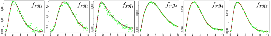
Figure 3: Laplace convolution $q$ (dotted red line) of the known kernel $g$ and the unknown function $f$, $n=100$ noisy observations of $q$ (green pluses) and estimated value of $q$ (black line). The choice of $f$ and $g$ used for each simulation are specified on each sub-figure by the convolution product. The noise level has been chosen as $\sigma_{0}(g_{j})/2$ for the three left figures and $\sigma_{0}(g_{j})/8$ for the three right figures.

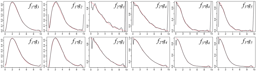
Figure 4: True unknown $f$ (red dotted line) and its estimate (plain black line) for $n=100$ (top line) and $n=250$ (bottom line).

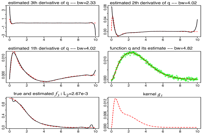
Figure 5: Example of estimation of unknown function $f_{3}$ with kernel $g_{5}$ using $n=250$ and $\sigma_{0}(g_{5})/4$. Here $r=3$. The top four sub-figures show true $q$ and its three first derivatives $q^{(s)}$, $s=1,2,3$ (dotted red lines) and their estimators (plain black lines). Selected bandwidths are specified for each estimator. Bottom left: the true function $f$ (dotted red line) and its estimate (plain black line). Bottom right: the kernel $g_{5}$.

For each combination of true function $f$, kernel $g$, sample size $n$ and the noise level, we ran 400 simulations and calculated mean square errors. In order to remove the influence of boundary effects (see comments above), we did not include 20% of the boundary points (10% at each boundary). The box-plots of the resulting mean square errors are presented on Figure 6. Table 1 shows the average mean square errors and standard deviations (in parentheses) over 400 simulation runs.

      

Figure 6: Box-plots of the mean square errors for $n=100$ (left) and $n=250$ (right), 400 simulation runs and each of the triplets $(g,f,\sigma_{0}(g))$. Each line represents a kernel from $g_{1}$ (top) to $g_{5}$ (bottom). Each column represents an unknown function $f$ from $f_{1}$ (left) to $f_{3}$ (right). In every sub-figure, going from left to right, each boxplot corresponds to a different noise level $\sigma_{0}(g_{j})/2^{i}$ for $i=0,\ldots,4$. The empirical risks are presented on log-scale with the basis 10.

$\hat{R}(\hat{f})$		i=0	i=1	i=2	i=3	i=4
$g_{1}$	$f_{1}$	1.6e-2 (9.5e-3)	4.1e-3 (2.5e-3)	9.9e-4 (6.6e-4)	2.9e-4 (1.7e-4)	7.6e-5 (4.7e-5)	$n=100$
	$f_{2}$	1.7e-2 (1.0e-2)	4.5e-3 (2.8e-3)	1.4e-3 (8.4e-4)	6.7e-4 (4.2e-4)	3.4e-4 (1.9e-4)
	$f_{3}$	1.5e-2 (9.6e-3)	4.0e-3 (2.6e-3)	1.4e-3 (9.0e-4)	7.4e-4 (4.4e-4)	3.6e-4 (1.7e-4)
$g_{2}$	$f_{1}$	2.3e-3 (1.1e-3)	6.9e-4 (4.6e-4)	2.2e-4 (8.8e-5)	6.1e-5 (2.2e-5)	1.5e-5 (5.5e-6)
	$f_{2}$	3.5e-3 (1.5e-3)	8.2e-4 (4.0e-4)	2.9e-4 (1.3e-4)	7.5e-5 (2.8e-5)	2.4e-5 (7.7e-6)
	$f_{3}$	2.1e-3 (1.4e-3)	8.6e-4 (4.4e-4)	2.9e-4 (1.1e-4)	7.2e-5 (2.8e-5)	2.5e-5 (7.8e-6)
$g_{3}$	$f_{1}$	1.2e-2 (3.7e-3)	2.4e-3 (1.0e-3)	1.3e-3 (3.6e-4)	8.7e-4 (1.4e-4)	7.4e-4 (7.2e-5)
	$f_{2}$	1.4e-2 (3.8e-3)	3.5e-3 (9.2e-4)	2.2e-3 (5.0e-4)	1.7e-3 (1.9e-4)	1.6e-3 (9.1e-5)
	$f_{3}$	1.0e-2 (3.6e-3)	4.3e-3 (1.4e-3)	1.2e-3 (3.7e-4)	8.2e-4 (1.5e-4)	7.1e-4 (7.3e-5)
$g_{4}$	$f_{1}$	2.2e-2 (1.2e-2)	6.3e-3 (3.3e-3)	1.2e-3 (8.3e-4)	4.2e-4 (2.4e-4)	1.2e-4 (6.5e-5)
	$f_{2}$	2.0e-2 (1.2e-2)	6.6e-3 (3.6e-3)	1.8e-3 (1.0e-3)	6.0e-4 (3.1e-4)	3.6e-4 (1.1e-4)
	$f_{3}$	2.1e-2 (1.2e-2)	5.7e-3 (3.5e-3)	1.8e-3 (1.0e-3)	5.5e-4 (3.0e-4)	3.0e-4 (1.1e-4)
$g_{5}$	$f_{1}$	3.2e-2 (1.7e-2)	9.4e-3 (4.6e-3)	2.8e-3 (1.2e-3)	5.3e-4 (3.2e-4)	1.6e-4 (9.9e-5)
	$f_{2}$	2.7e-2 (1.7e-2)	9.8e-3 (4.5e-3)	2.9e-3 (1.5e-3)	8.8e-4 (4.7e-4)	3.4e-4 (1.4e-4)
	$f_{3}$	2.6e-2 (1.7e-2)	8.1e-3 (4.8e-3)	2.9e-3 (1.5e-3)	8.3e-4 (4.8e-4)	3.4e-4 (1.4e-4)
$g_{1}$	$f_{1}$	5.5e-3 (3.4e-3)	1.6e-3 (9.0e-4)	4.1e-4 (2.3e-4)	1.2e-4 (5.7e-5)	5.9e-5 (2.2e-5)	$n=250$
	$f_{2}$	7.0e-3 (3.8e-3)	1.9e-3 (1.2e-3)	1.0e-3 (5.6e-4)	5.3e-4 (2.6e-4)	1.6e-4 (9.1e-5)
	$f_{3}$	6.5e-3 (3.9e-3)	1.8e-3 (1.1e-3)	1.0e-3 (5.4e-4)	5.0e-4 (2.6e-4)	1.5e-4 (8.4e-5)
$g_{2}$	$f_{1}$	1.4e-3 (5.2e-4)	2.7e-4 (1.2e-4)	9.1e-5 (5.4e-5)	3.5e-5 (1.9e-5)	1.0e-5 (3.1e-6)
	$f_{2}$	1.2e-3 (5.4e-4)	3.7e-4 (1.8e-4)	1.3e-4 (5.2e-5)	3.8e-5 (1.1e-5)	1.1e-5 (3.2e-6)
	$f_{3}$	1.0e-3 (4.9e-4)	3.9e-4 (1.8e-4)	1.2e-4 (4.8e-5)	3.8e-5 (1.1e-5)	1.1e-5 (3.4e-6)
$g_{3}$	$f_{1}$	3.4e-3 (1.7e-3)	1.2e-3 (4.1e-4)	3.8e-4 (2.2e-4)	1.7e-4 (4.7e-5)	5.8e-5 (1.4e-5)
	$f_{2}$	3.6e-3 (2.2e-3)	1.4e-3 (3.8e-4)	2.3e-4 (1.1e-4)	9.6e-5 (3.4e-5)	4.8e-5 (1.2e-5)
	$f_{3}$	6.3e-3 (1.4e-3)	1.0e-3 (7.1e-4)	2.1e-4 (1.1e-4)	6.1e-5 (2.9e-5)	3.3e-5 (1.2e-5)
$g_{4}$	$f_{1}$	8.9e-3 (4.5e-3)	2.7e-3 (1.1e-3)	5.8e-4 (3.0e-4)	1.6e-4 (8.6e-5)	4.9e-5 (2.3e-5)
	$f_{2}$	8.8e-3 (4.6e-3)	2.9e-3 (1.5e-3)	8.2e-4 (3.8e-4)	2.8e-4 (1.5e-4)	1.6e-4 (9.6e-5)
	$f_{3}$	7.7e-3 (4.8e-3)	3.2e-3 (1.3e-3)	8.1e-4 (3.7e-4)	2.9e-4 (1.9e-4)	1.9e-4 (9.6e-5)
$g_{5}$	$f_{1}$	1.5e-2 (7.0e-3)	4.1e-3 (2.0e-3)	7.4e-4 (4.4e-4)	2.7e-4 (1.4e-4)	7.2e-5 (4.0e-5)
	$f_{2}$	1.3e-2 (6.7e-3)	4.6e-3 (1.9e-3)	1.3e-3 (6.4e-4)	4.3e-4 (2.3e-4)	2.4e-4 (9.9e-5)
	$f_{3}$	1.4e-2 (6.9e-3)	3.5e-3 (1.9e-3)	1.2e-3 (5.9e-4)	4.1e-4 (2.2e-4)	2.2e-4 (9.4e-5)

Table 1: Average (over 400 simulation runs) mean square errors and standard deviations (in parentheses) for kernels $g_{1}$ to $g_{5}$ and unknown function $f_{1}$ to $f_{3}$, for $n=100$ (upper part) and $n=250$ (lower part) and for the noise level equal to $\sigma_{0}(g_{j})/2^{i}$, $j=1,\ldots,5;\;i=0,\ldots,4$.

4 Discussion

In the present paper, we consider Laplace deconvolution problem with discrete noisy data observed on the interval whose length $T_{n}$ may increase with the sample size $n$. Although this problem arises in a variety of applications, to the best of our knowledge, it has been given very little attention by the statistical community. Our objective was to fill this gap and to provide statistical analysis of Laplace deconvolution problem with noisy discrete data.

The main contribution of the paper is explicit construction of a rate-optimal (in the minimax sense) Laplace deconvolution estimator which is adaptive to the regularity of the unknown function. We show that the original Laplace deconvolution problem can be reduced to nonparametric estimation of a regression function and its derivatives on the interval of growing length $T_{n}$. Although the latter problem has been well studied on a finite interval, the asymptotic increase of its length as the sample size grows raises a new challenge. Whereas the forms of the estimators remains standard, the choices of the parameters and the minimax convergence rates, which are expressed in terms of $T_{n}^{2}/n$ in this case, are affected by the asymptotic growth of the length of the interval.

In the present paper, we use kernel estimators with a global bandwidth adaptively chosen by the Lepski procedure (e.g., Lepski, 1991) and establish asymptotic minimaxity of the resulting Laplace deconvolution estimator over a wide range of Sobolev classes. One can, however, apply other types of estimators (e.g., local polynomial regression, splines or wavelets). In particular, we believe that the use of wavelet-based methods can extend the adaptive minimaxity range from Sobolev to more general Besov classes.

We illustrate the theory by examples of construction of explicit expressions for estimators of $f$ based on observations governed by equation (1.3) with various kernels. Simulation study shows, that, in addition to providing asymptotic optimality, the proposed Laplace deconvolution estimator demonstrates good finite sample performance.

The present paper provides the first comprehensive statistical treatment of Laplace deconvolution problem, though a number of open questions remain beyond its scope. In particular, an interesting challenge would be to study Laplace deconvolution with an unstable resolvent, where Assumption (A2) does not hold. Another important problem would be to study the equation (1.3) when the kernel $g$ is not completely known and is estimated from observations.

5 Appendix

Throughout the proofs we use $C$ to denote a generic positive constant, not necessarily the same each time it is used, even within a single equation.

Proof of Theorem 1

Although the rates are derived by standard methods described in, e.g., Tsybakov (2009), the challenging part of the proof is constructing the set of test functions and, subsequently, producing upper bounds for the Kullback-Leibler divergence.

The main idea of the proof is to find a subset of functions ${\cal F}\subset W^{m}(A)$ such that for any pair $f_{1},\;f_{2}\in{\cal F}$,

$$\|f_{1}-f_{2}\|^{2}_{L_{2}([0,T_{n}])}\geq 4C(T^{2}_{n}n^{-1})^{2m/(2(m+r)+1)}$$ (5.1)

and the Kullback-Leibler divergence

$${\mathbb{K}}({\mathbb{P}}_{f_{1}},{\mathbb{P}}_{f_{2}})=\frac{||\mbox{\boldmath$q$}_{1}-\mbox{\boldmath$q$}_{2}||^{2}_{\mathbb{R}^{n}}}{2\sigma^{2}}\leq\frac{\log{\rm card}({\cal F})}{16},$$ (5.2)

where $\log$ stands for natural logarithm and vectors $\mbox{\boldmath$q$}_{j}$, $j=1,2$, have components $\mbox{\boldmath$q$}_{ji}=(g\ast f_{j})(t_{i})$, $i=1,...,n$. The result will then follow immediately from Lemma A.1 of Bunea, Tsybakov and Wegkamp (2007):

Lemma 1.

[Bunea, Tsybakov, Wegkamp (2007), Lemma A.1] Let ${\cal F}$ be a set of functions of cardinality $\mbox{card\,}({\cal F})\geq 2$ such that
(i) $\|f_{1}-f_{2}\|^{2}\geq 4\delta^{2}\quad$ for any $f_{1},f_{2}\in{\cal F}$,  $f_{1}\neq f_{2}$,
(ii) the Kullback divergences ${\mathbb{K}}({\mathbb{P}}_{f_{1}},{\mathbb{P}}_{f_{2}})$ between the measures ${\mathbb{P}}_{f_{1}}$ and ${\mathbb{P}}_{f_{2}}$ satisfy the inequality ${\mathbb{K}}({\mathbb{P}}_{f_{1}},{\mathbb{P}}_{f_{2}})\leq(1/16)\log(\mbox{card\,}({\cal F}))\quad$ for any $f_{1},f_{2}\in{\cal F}$.
Then, for some absolute positive constant $C$,

$$\inf_{\tilde{f}_{n}}\sup_{f\in\ {\cal F}}{\mathbb{E}}_{f}\|\tilde{f}_{n}-f\|^{2}\geq C\delta^{2},$$

where the infimum is taken over all estimates $\tilde{f}_{n}$ of $f$.

Without loss of generality, let us assume that the points are equally spaced, i.e. $t_{i}-t_{i-1}=T_{n}/n$, $i=1,...,n$. To construct such a subset ${\cal F}$, define integers $M_{n}\geq 8$ and $N=\left[\frac{n}{M_{n}}\right]$, the largest integer which does not exceed $n/M_{n}$. Let $\lambda_{n}=NT_{n}/n$ and define points $z_{l}=l\,\lambda_{n}$, $l=0,1,...,M_{n}$. Note that the latter implies that points of observation $t_{j}=j\,T_{n}/n$ in equation (1.3) are related to $z_{l}$ as $z_{l}=t_{j}$ where $j=Nl$ for $l=1,...,M_{n}$ and $j\leq NM_{n}$. Note also that $\frac{T_{n}}{2M_{n}}\leq\lambda_{n}\leq\frac{T_{n}}{M_{n}}$.

Let $k(\cdot)$ be an infinitely differentiable function with $supp(k)=[0,1]$ and such that

$$\int_{0}^{1}x^{j}k(x)dx=0,j=0,...,r-1,\ \ \ \int_{0}^{1}x^{r}k(x)dx\neq 0.$$ (5.3)

Introduce functions

$$\varphi_{j}(x)=L\,\frac{\lambda_{n}^{m}}{\sqrt{T_{n}}}\,k\left(\frac{x-z_{j-1}}{\lambda_{n}}\right)\ \ \ l=1,...,M_{n},$$

where the constant $L>0$ will be defined later. Note that $\varphi_{j}$ have non-overlapping supports, where $supp(\varphi_{j})=[z_{j-1},z_{j}]$.

Consider the set of all binary sequences of the length $M_{n}\geq 8$:

$$\Omega=\big{\{}\mbox{$\omega$}=(\omega_{1},...,\omega_{M_{n}}),\ \ \omega_{j}=\{0,1\}\big{\}}=\{0,1\}^{M_{n}}$$

and the corresponding subset of functions

$${\cal F}=\{f_{\omega}:f_{\omega}(t)=\sum_{j=1}^{M_{n}}w_{j}\varphi_{j}(t),\;\omega\in\tilde{\Omega}\}.$$ (5.4)

Here $\tilde{\Omega}\subset\Omega$ is such that $\log_{2}{\rm card}(\tilde{\Omega})\geq M_{n}/8$ and the Hamming distance $\rho(\mbox{$\omega$}_{1},\mbox{$\omega$}_{2})=\sum_{j=1}^{M_{n}}\mathbb{I}\{\mbox{$\omega$}_{1j}\neq\mbox{$\omega$}_{2j}\}\geq M_{n}/8$ for any pair $\mbox{$\omega$}_{1},\mbox{$\omega$}_{2}\in\tilde{\Omega}$ (see, e.g., Lemma 2.9 of Tsybakov (2009) for construction of $\tilde{\Omega}$).

We now need to show that ${\cal F}$ in (5.4) is exactly the required set. Note first that since the supports of $\varphi_{j}$ are non-overlapping, for any $f_{\omega}\in{\cal F}$ a straightforward calculus yields

$$||f_{\omega}||^{2}_{L_{2}([0,T_{n}])}\leq\sum_{j=1}^{M_{n}}||\varphi_{j}||^{2}=L^{2}\frac{\lambda_{n}^{2s+1}}{T_{n}}M_{n}||k||^{2}=L^{2}\lambda^{2m}||k||^{2}\leq L^{2}||k||^{2}$$

Similarly,

$$||f^{(m)}_{\omega}||^{2}_{L_{2}([0,T_{n}])}\leq\sum_{j=1}^{M_{n}}||\varphi^{(m)}_{j}||^{2}=\frac{L^{2}}{T_{n}}m\lambda_{n}||k^{(s)}||^{2}=L^{2}||k^{(m)}||^{2}<\infty$$

and therefore $f_{\omega}\in W^{(m)}(A)$, where $A=L||k||_{W^{m}}$. Furthermore,

$$||f_{\omega_{1}}-f_{\omega_{2}}||^{2}_{L_{2}([0,T_{n}])}=L^{2}\frac{\lambda_{n}^{2m+1}}{T_{n}}||k||^{2}\rho(\mbox{$\omega$}_{1},\mbox{$\omega$}_{2})\geq L^{2}\frac{\lambda_{n}^{2m+1}}{T_{n}}\frac{M_{n}}{8}\geq 4C\lambda_{n}^{2m}$$

and (5.1) holds provided $\lambda_{n}\geq C(T^{2}_{n}n^{-1})^{-1/(2(m+r)+1)}$ for some positive constant $C$.

To verify (5.2), note that

$${\mathbb{K}}(P_{1},P_{2})=\frac{1}{2\sigma^{2}}\ \sum_{i=1}^{n}\left[q_{1}(t_{i})-q_{2}(t_{i})\right]^{2}\leq\frac{1}{\sigma^{2}}\sum_{j=1}^{2}Q(f_{j})$$ (5.5)

where, suppressing index $j$, we write

$$Q(f) = \ \sum_{i=1}^{n}\left[\int_{0}^{t_{i}}g(t_{i}-x)f(x)dx\right]^{2}=\frac{L^{2}\lambda_{n}^{2m}}{T_{n}}\ \sum_{i=1}^{n}\left[\sum_{l=1}^{M_{n}}\omega_{l}^{(j)}\int_{0}^{t_{i}}g(t_{i}-x)k\left(\frac{x-z_{l-1}}{\lambda_{n}}\right)dx\right]^{2}.$$

In order to obtain an upper bound for $Q(f)$ we need the following supplementary lemma, the proof of which is presented at the end of the section.

Lemma 2.

Introduce functions $K_{j}(x)$ using the following recursive relation

$$K_{1}(x)=\int_{0}^{x}k(t)dt,\ \ K_{j}(x)=\int_{0}^{x}K_{j-1}(t)dt,\ \ j=2,...,r.$$ (5.6)

Then, under condition (5.3), functions $K_{j}(x)$, $j=1,...,r$, are uniformly bounded and $K_{j}(1)=0$, $j=1,\ldots,r$. Moreover,

$$\int_{0}^{t_{i}}g(t_{i}-x)k\left(\frac{x-z_{l-1}}{\lambda_{n}}\right)dx = \lambda_{n}^{r}\left[B_{r}K_{r}\left(\frac{t_{i}-z_{l-1}}{\lambda_{n}}\right){\mathbb{I}}(z_{l-1}\leq y_{i}\leq z_{l})\right.$$ (5.7)

$$+ \left.\int_{\min(z_{l-1},t_{i})}^{\min(z_{l},t_{i})}g^{(r)}(t_{i}-x)K_{r}\left(\frac{x-z_{l-1}}{\lambda_{n}}\right)dx\right].$$

Applying equation (5.7) to the integral in $Q(f)$, obtain

$$Q(f)\leq 2L^{2}\lambda_{n}^{2m+2r}T_{n}^{-1}\,(\Delta_{1}+\Delta_{2})$$ (5.8)

where

$$\Delta_{1} = \sum_{i=1}^{n}\left[\sum_{l=1}^{M_{n}}B_{r}\ K_{r}\left(\frac{t_{i}-z_{l-1}}{\lambda_{n}}\right){\mathbb{I}}(z_{l-1}\leq y_{i}\leq z_{l})\right]^{2},$$

$$\Delta_{2} = \sum_{i=1}^{n}\left[\sum_{l=1}^{M_{n}}\int_{\min(z_{l-1},t_{i})}^{\min(z_{l},t_{i})}g^{(r)}(t_{i}-x)K_{r}\left(\frac{x-z_{l-1}}{\lambda_{n}}\right)dx\right]^{2}.$$

Observe that for any $t$ and any $l_{1}$ and $l_{2}$ such that $l_{1}\neq l_{2}$, one has $K_{r}(\lambda_{n}^{-1}(t-z_{l_{1}}))K_{r}(\lambda_{n}^{-1}(t-z_{l_{2}}))=0$. Also, for each $i$, $K_{r}(\lambda_{n}^{-1}(ti-z_{l}))\neq 0$ for only one value of $l$, namely, for $l=[i/N]+1$ where $[x]$ is the largest integer which does not exceed $x$. Therefore,

$$\Delta_{1}\leq B_{r}^{2}\sum_{i=1}^{n}K_{r}^{2}\left(\frac{t_{i}-z_{[i/N]}}{\lambda_{n}}\right)\leq n\,\,B_{r}^{2}\|K_{r}\|^{2}_{\infty},$$ (5.9)

where $\|\cdot\|_{\infty}$ is the supremum norm. In order to obtain an upper bound for $\Delta_{2}$, observe that for any nonnegative function $F(x)$ one has

$$\int_{\min(z_{l-1},t_{i})}^{\min(z_{l},t_{i})}F(x)dx\leq\int_{z_{l-1}}^{z_{l}}F(x)dx.$$

Hence, we derive

$$\Delta_{2} \leq \sum_{i=1}^{n}\left[\sum_{l=1}^{M_{n}}\int_{z_{l-1}}^{z_{l}}\left|g^{(r)}(t_{i}-x)K_{r}\left(\frac{x-z_{l-1}}{\lambda_{n}}\right)\right|dx\right]^{2}$$ (5.10)

$$\leq \sum_{i=1}^{n}\|K_{r}\|^{2}_{\infty}\left[\sum_{l=1}^{M_{n}}\int_{z_{l-1}}^{z_{l}}|g^{(r)}(t_{i}-x)|dx\right]^{2}\leq n\,\|g^{(r)}\|^{2}\|K_{r}\|^{2}_{\infty}.$$

Combining formulae (5.5)–(5.10), we obtain that, in order to satisfy the condition (5.2), we need the following inequality to hold

$${\mathbb{K}}({\mathbb{P}}_{f_{1}},{\mathbb{P}}_{f_{2}})\leq\frac{2L^{2}\lambda_{n}^{2m+2r}n}{\sigma^{2}T_{n}}\,\|K_{r}\|^{2}_{\infty}[B_{r}^{2}+\|g^{(r)}\|^{2}_{2}]\leq\frac{1}{16}\,\frac{M_{n}\log 2}{8}.$$ (5.11)

Note that $\frac{T_{n}}{M_{n}}\left(1-\frac{T_{n}}{M_{n}}\right)\leq\lambda_{n}\leq\frac{T_{n}}{M_{n}}$. Choosing $M_{n}=Cn^{1/(2(m+r)+1)}T_{n}^{(2(m+r)-1)/(2(m+r)+1)}$ and observing that $T_{n}/M_{n}\rightarrow 0$ as $n\rightarrow\infty$, obtain $\lambda_{n}\geq T_{n}/(2M_{n})\geq C(T^{2}_{n}n^{-1})^{1/(2(m+r)+1)}$. Therefore, both conditions (5.1) and (5.2) hold and theorem is proved.
$\Box$

Proof of Theorem 2

To prove Theorem 2 we use the following Lemma 3 which can be viewed as a version of Theorem 7.2.4 of Gripenberg, Londen and Staffans (1990, Chapter 7) adapted to our notations.

Lemma 3.

Let $s_{g}$ be such that

$$\inf_{Re(s)=s_{g}}|\tilde{g}(s)|>0\ \ \ \mbox{and}\ \ \ \ \lim_{\stackrel{{\scriptstyle|s|\rightarrow\infty}}{{Re(s)\geq s_{g}}}}|s^{r}\tilde{g}(s)|>0.$$ (5.12)

Then, solution $\phi(\cdot)$ of equation (2.4) can be presented as

$$\phi(t)=\sum_{l=0}^{L}\sum_{j=0}^{\alpha_{l}-1}\frac{a_{l,j}}{j!}t^{j}e^{s_{l}t}+\phi_{1}(t)$$ (5.13)

where $L$ is the total number of distinct zeros $s_{l}$ of $s^{r}\tilde{g}(s)$ such that $Re(s_{l})>Re(s_{g})$, $\alpha_{l}$ is the order of zero $s_{l}$ and $\phi_{1}\in L_{1}$.

Choose $s_{g}$ such that $s^{*}<s_{g}<0$. Then, the first condition in (5.12) immediately follows from Assumption (A2). To validate the second assumption in (5.12), note that for $s=s_{1}+is_{2}$ conditions $Re(s)\geq s_{g}$ and $|s|\rightarrow\infty$ imply that either $s_{1}\rightarrow\infty$ or $|s_{2}|\rightarrow\infty$, or both. Recall that $s^{r}\tilde{g}(s)=B_{r}+\widetilde{G^{(r)}}(s)$. If $s_{1}\rightarrow\infty$, no matter whether $s_{2}$ is finite or $s_{2}\rightarrow\infty$, one has

$$\lim_{Re(s)\rightarrow\infty}|s^{r}\tilde{g}(s)|=\lim_{Re(s)\rightarrow\infty}|B_{r}+\int_{0}^{\infty}g^{(r)}(t)e^{-st}dt|=|B_{r}|>0.$$ (5.14)

If $s_{1}$ is finite, $s_{1}\geq s_{g}$, and $|s_{2}|\rightarrow\infty$, then Laplace transform $\widetilde{g^{(r)}}(s)=\int_{0}^{\infty}g^{(r)}(t)e^{-st}dt$ is equal to Fourier transform ${\cal F}[g^{(r)}(t)e^{-s_{1}t}](s_{2})$ of function $g^{(r)}(t)e^{-s_{1}t}$ at the point $s_{2}$. Since $g^{(r)}(t)e^{-s_{1}t}\in L_{1}(\mathbb{R}^{+})$, one obtains

$$\lim_{|s_{2}|\rightarrow\infty}\int_{0}^{\infty}g^{(r)}(t)e^{-st}dt=\lim_{|s_{2}|\rightarrow\infty}{\cal F}[g^{(r)}(t)e^{-s_{1}t}](s_{2})=0,$$

and (5.14) holds again. Hence, the second assumption in (5.12) is valid, and Lemma 3 can be applied.

Note that, under Assumption (A2), $\tilde{g}(s)$ has no zeros with $Re(s)>s_{g}$ and, therefore, $s^{r}\tilde{g}(s)$ has a single zero of $r$-th order at $s=0$. Lemma 3 yields then that $\phi(t)=\phi_{0}(t)+\phi_{1}(t)$, where

$$\phi_{0}(t)=\sum_{j=0}^{r-1}\frac{a_{0,j}}{j!}t^{j},\;\;\;a_{0,j}=\phi^{(j)}(0),$$ (5.15)

and integrating by parts, one has

$$\int_{0}^{t}q^{(r)}(t-\tau)\phi_{0}(\tau)d\tau=\sum_{j=0}^{r-1}\phi_{0}^{(r-j-1)}(0)q^{(j)}(t),$$ (5.16)

that completes the proof of (2.8).

In order to prove (2.9) – (2.12), note that it follows from equation (2.6) that $\tilde{\phi}(s)$ has poles $s_{l}$, $l=0,\ldots,M$, of respective orders $\alpha_{l}$, where $s_{0}=0$ and $\alpha_{0}=r$. Since, by (5.14), one has

$$\lim_{\stackrel{{\scriptstyle|s|\rightarrow\infty}}{{Re(s)\geq s_{g}}}}|s^{r}\tilde{g}(s)|>0$$

and, therefore, $\tilde{\phi}$ does not have a pole at infinity. Then, $\tilde{\phi}$ is a rational function and, consequently, can be represented using Cauchy integral formula

$$\tilde{\phi}(s)=-\frac{1}{2\pi i}\sum_{l=0}^{M}\oint_{C_{l}}\frac{\tilde{\phi}(z)}{z-s}dz$$

where $C_{l}$, $l=0,...,M$, is a circle around the pole $s_{l}$ such that this circle does not enclose any other pole of $\tilde{\phi}$ (see LePage, 1961, Section 5.14). Using Laurent expansion of $\tilde{\phi}(z)$ around $s_{l}$, we have

$$I_{l}(s)=\frac{1}{2\pi i}\oint_{C_{l}}\frac{\tilde{\phi}(z)}{z-s}dz=-\sum_{j=0}^{\alpha_{l}-1}\frac{1}{(s-s_{l})^{j+1}}\ \frac{1}{(\alpha_{l}-1-j)!}\ \frac{d^{\alpha_{l}-j-1}}{ds^{\alpha_{l}-j-1}}\left[(s-s_{l})^{\alpha_{l}}\tilde{\phi}(s)\right]\Bigg{|}_{s=s_{l}}$$

Combining the last two expressions and taking inverse Laplace transform of $\tilde{\phi}(s)$ yields

$$\phi(t)=\sum_{l=0}^{M}\sum_{j=0}^{\alpha_{l}-1}\frac{a_{l,j}}{j!}t^{j}e^{s_{l}t}=\phi_{0}(t)+\phi_{1}(t),$$

where $\phi_{0}$ is given by (5.15), same as before, and

$$\phi_{1}(t)=\sum_{l=1}^{M}\sum_{j=0}^{\alpha_{l}-1}\frac{a_{l,j}}{j!}t^{j}e^{s_{l}t}.$$ (5.17)

Repeat calculations in (5.16) and also note that, by similar considerations, for every $j=0,...,\alpha_{l}-1$, one can write

$$\int_{0}^{t}q^{(r)}(t-x)x^{j}e^{s_{l}x}dx=\sum_{k=0}^{r-1}q^{(r-k-1)}(t)\,\frac{d^{k}}{dx^{k}}\left[x^{j}e^{s_{l}x}\right]\Bigg{|}_{x=0}+\int_{0}^{t}q(t-x)\frac{d^{(r-1)}}{dx^{(r-1)}}\left[x^{j}e^{s_{l}x}\right]dx.$$

To complete the proof, evaluate the derivatives, observe that

$$\frac{d^{k}}{dx^{k}}\left[x^{j}e^{s_{l}x}\right]\Bigg{|}_{x=0}={k\choose j}\,s_{l}^{k-j}$$

and interchange summation with respect to $j$ and $k$.
$\Box$

Proof of Theorem 3

Since the estimator (2.14) is just a particular form of the estimator (2.13), it is sufficient to carry out the proof for the estimator (2.13) of $f$. From (2.8), one immediately obtains

$$E||\hat{f}_{n}-f||^{2}_{[0,T_{n}]}\leq\frac{r+2}{B^{2}_{r}}\left(E||\widehat{q_{\hat{\lambda}_{r,n}}^{(r)}}-q^{(r)}||^{2}_{[0,T_{n}]}\right. + \sum_{j=0}^{r-1}a^{2}_{0,r-1-j}E||\widehat{q_{\hat{\lambda}_{j,n}}^{(j)}}-q^{(j)}||^{2}_{[0,T_{n}]}$$ (5.18)

$$+ \left.||\widehat{q_{\hat{\lambda}_{r,n}}^{(r)}}\ast\phi_{1}-q^{(r)}\ast\phi_{1}||^{2}_{[0,T_{n}]}\right),$$

where $\widehat{q_{\hat{\lambda}_{j,n}}^{(j)}},\;j=0,\ldots,r$ are given in (2.19).

The proof is based on the following proposition which provides upper bounds for the risks $E||\widehat{q_{\hat{\lambda}_{j,n}}^{(j)}}-q^{(j)}||^{2}_{[0,T_{n}]},\;j=0,...,r$ in (5.18).

Proposition 1.

Let condition (2.1) and Assumptions (A1)-(A4) hold. Let kernel $K_{j}$ be of order $(L,j)$, where $L>r$ and $0\leq j\leq r$, and satisfies Assumptions (K1) and (K2). Then, for all $A^{\prime}>0$,

$$\sup_{q\in W^{m+r}(A^{\prime})}\,E||\widehat{q_{\hat{\lambda}_{j,n}}^{(j)}}-q^{(j)}||^{2}_{[0,T_{n}]}=O\left(\left(\frac{T_{n}^{2}}{n}\right)^{\frac{2(r+m-j)}{2(r+m)+1}}\right).$$ (5.19)

In particular, Proposition 1 implies that the errors of estimating $q^{(j)}$ in (5.18) are dominated by the estimation error of the highest order derivative $q^{(r)}$. Furthermore, $\phi_{1}\in L_{1}$ (see Theorem 2) and, therefore,

$$\|\widehat{q_{\hat{\lambda}_{r,n}}^{(r)}}\ast\phi_{1}-q^{(r)}\ast\phi_{1}\|_{2}\leq\|\phi_{1}\|_{1}\cdot\|\widehat{q_{n}^{(r)}}-q^{(r)}\|_{2}=O\left(\|\widehat{q_{\hat{\lambda}_{r,n}}^{(r)}}-q^{(r)}\|_{2}\right)$$

(see also Theorem 2.2.2 of Gripenberg, Londen and Staffans, 1990).

Thus, (5.18) and Proposition 1 yield

$$E||\hat{f}_{n}-f||^{2}_{[0,T_{n}]}=O\left(E||\widehat{q_{\hat{\lambda}_{r,n}}^{(r)}}-q^{(r)}||^{2}_{[0,T_{n}]}\right)=O\left(\left(\frac{T_{n}^{2}}{n}\right)^{\frac{2m}{2m+2r+1}}\right)$$

$\Box$

Proof of Proposition 1

For simplicity of notations we drop the index $n$ in $\hat{\lambda}_{j,n}$.

Recall that under Assumptions (A1)-(A3), $q\in W^{r+m}$ (see Section 2.3). By the standard asymptotic calculus for kernel estimation (see, e.g., Gasser and Müller, 1984) for estimator (2.15) and any interior point $t$ of $(0,T_{n})$, one then has

$$Var\left(\widehat{q_{\lambda}^{(j)}}(t)\right)=\frac{\sigma^{2}}{\lambda_{j}^{2(j+1)}}\ \sum_{i=1}^{n}(t_{i}-t_{i-1})^{2}K_{j}^{2}\left(\frac{t_{i}-t}{\lambda_{j}}\right)=\frac{\sigma^{2}}{\lambda_{j}^{2j+1}}\frac{T_{n}}{n}\int K_{j}^{2}(u)du\;(1+o(1)).$$

The required boundary corrections ensure the same order of error for the values $t$ close to the boundaries (Gasser and Müller, 1984) and the integrated variance then is

$$V_{j}(\lambda_{j})=\int_{0}^{T_{n}}Var\left(\widehat{q_{\lambda_{j}}^{(j)}}(t)\right)dt=V_{0j}\ \frac{T^{2}_{n}}{\lambda_{j}^{2j+1}n}\;(1+o(1)),$$ (5.20)

where $V_{0j}=\sigma^{2}||K_{j}||^{2}$. Similarly, the integrated squared bias can be written as

$$B_{j}^{2}(\lambda_{j},q)=\int_{0}^{T_{n}}\left(E\left(\widehat{q_{\lambda_{j}}^{(j)}}(t)\right)-q^{(j)}(t)\right)^{2}dt=B_{0j}\lambda_{j}^{2(r+m-j)}(1+o(1)),$$ (5.21)

where $B_{0j}=B^{-1}_{0}||q^{(r+m)}||^{2}||K_{j}||^{2}$ and $B_{0}=2\left((r+m-1)!\right)^{2}(2(r+m)-1)(2(r+m)+1)$. Hence,

$$\sup_{q\in W^{m+r}(A)}E||\widehat{q_{\lambda_{j}}^{(j)}}-q^{(j)}||^{2}_{L_{2}([0,T_{n})]}=\sup_{q\in W^{m+r}(A)}\left(V_{j}(\lambda_{j})+B_{j}^{2}(\lambda_{j},q)\right)=O\left(\frac{T^{2}_{n}}{\lambda_{j}^{2j+1}n}\right)+O\left(\lambda_{j}^{2(r+m-j)}\right).$$ (5.22)

It follows from (5.20) and (5.21) that the asymptotically optimal bandwidth that minimizes $E||\widehat{q_{\lambda_{j}}^{(j)}}-q^{(j)}||^{2}_{L_{2}([0,T_{n}])}$ is

$$\lambda_{j}^{*}=O\left(\left(\frac{T_{n}^{2}}{n}\right)^{\frac{1}{2(r+m)+1}}\right)$$ (5.23)

and the corresponding risk of estimating $q^{(j)}$ is given by

$$\sup_{q\in W^{m+r}(A^{\prime})}E||\widehat{q_{\lambda_{j}^{*}}^{(j)}}-q^{(j)}||^{2}_{L_{2}([0,T_{n}])}=O\left(\left(\frac{T_{n}^{2}}{n}\right)^{\frac{2(r+m-j)}{2(r+m)+1}}\right).$$ (5.24)

Now we need to prove that (5.24) remains valid when $\lambda_{j}^{*}$ is replaced by $\hat{\lambda}_{j}$ selected by Lepski procedure, that is,

$$\sup_{q\in W^{m+r}(A^{\prime})}\,E||\widehat{q_{\hat{\lambda}_{j}}^{(j)}}-q^{(j)}||^{2}=O\left(\left(\frac{T_{n}^{2}}{n}\right)^{\frac{2(r+m-j)}{2(r+m)+1}}\right)$$

for all $A^{\prime}>0$. Set $d_{j}$ and $\lambda^{*}_{j}$ in (5.23) to be, respectively,

$$d_{j}=\frac{C_{j}-\mu||K_{j}||}{2||K_{j}||},\quad\lambda^{*}_{j}=\left(d_{j}^{2}\ \frac{\sigma^{2}B_{0}}{2(A^{\prime})^{2}}\,\frac{T_{n}^{2}}{n}\right)^{\frac{1}{2(r+m)+1}},$$

where $C_{j}$ is defined in (2.18). Note that

$$E\|\widehat{q_{\hat{\lambda}_{j}}^{(j)}}-q^{(j)}\|^{2}=E\left\{\|\widehat{q_{\hat{\lambda}_{j}}^{(j)}}-q^{(j)}\|^{2}I(\hat{\lambda}_{j}\geq\lambda^{*}_{j})\right\}+E\left\{\|\widehat{q_{\hat{\lambda}_{j}}^{(j)}}-q^{(j)}\|^{2}I(\hat{\lambda}_{j}<\lambda^{*}_{j})\right\}=\Delta_{1}+\Delta_{2}.$$

For $\hat{\lambda}_{j}\geq\lambda^{*}_{j}$, equations (5.24) and (2.17) imply that uniformly over $q\in W^{m+r}(A^{\prime})$

$$\Delta_{1} \leq 2E\left\{\|\widehat{q_{\hat{\lambda}_{j}}^{(j)}}-q_{{\lambda}^{*}_{j}}^{(j)}\|^{2}I(\hat{\lambda}_{j}>\lambda^{*}_{j})\right\}+2E\left\{\|\widehat{q_{\hat{\lambda}^{*}_{j}}^{(j)}}-q^{(j)}\|^{2}I(\hat{\lambda}_{j}>\lambda^{*}_{j})\right\}$$ (5.25)

$$= O\left(n^{-1}T_{n}^{2}(\lambda^{*}_{j})^{-(2j+1)}\right)+O\left((n^{-1}T_{n}^{2})^{-\frac{2(r+m-j)}{2(r+m)+1}}\right)=O\left((n^{-1}T_{n}^{2})^{-\frac{2(r+m-j)}{2(r+m)+1}}\right).$$

For $(n^{-1}T_{n}^{2})^{\frac{1}{2j+1}}\leq\hat{\lambda}_{j}<\lambda^{*}_{j}$, by direct calculus similar to that carried out above, one can show that

$$\sup_{q\in W^{m+r}(A)}\,E\|\widehat{q_{\hat{\lambda}_{j}}^{(j)}}-q^{(j)}\|^{4} = O\left((\lambda^{*}_{j})^{-2(2j+1)}n^{-2}T_{n}^{4}\right)+O((\lambda^{*}_{n})^{4(r+m-j)})=O(1).$$

Hence,

$$\sup_{q\in W^{m+r}(A)}\Delta_{2} \leq \sup_{q\in W^{m+r}(A)}\sqrt{E\|\widehat{q_{\hat{\lambda}_{j}}^{(j)}}-q^{(j)}\|^{4}}\ \sqrt{P(\hat{\lambda}_{j}<\lambda^{*}_{j})}$$ (5.26)

$$= O\left(\sup_{q\in W^{m+r}(A)}\sqrt{P(\hat{\lambda}_{j}<\lambda^{*}_{j})}\right).$$

If $\lambda^{*}_{j}>\hat{\lambda}_{j}$, it follows from definition (2.17) of $\hat{\lambda}_{j}$ that there exists $\tilde{h}<\lambda^{*}_{j}$ such that $\|\widehat{q_{\lambda^{*}_{j}}^{(j)}}-\widehat{q_{\tilde{h}}^{(j)}}\|^{2}>4\,C_{j}^{2}n^{-1}\sigma^{2}T_{n}^{2}\tilde{h}^{-(2j+1)},$ where, by (2.18) and definition of $d_{j}$, we have $C_{j}=\|K_{j}\|(\mu+2d_{j})$. It follows from (5.20) and (5.21) that, for all $h<\lambda^{*}_{j}$, the variance term dominates the squared bias, that is,

$$\sup_{q\in W^{m+r}(A^{\prime})}\,\|E\widehat{q_{h}^{(j)}}-q^{(j)}\|^{2}\leq d_{j}^{2}\sigma^{2}\|K_{j}\|^{2}n^{-1}T_{n}^{2}h^{-(2j+1)}.$$

Hence, for all $\tilde{h}<\lambda^{*}_{j}$ and $q\in W^{m+r}(A^{\prime})$, one has

$$P\left(\|\widehat{q_{\lambda^{*}_{j}}^{(j)}}-\widehat{q_{\tilde{h}}^{(j)}}\|^{2}>4\,C_{j}^{2}n^{-1}\sigma^{2}T_{n}^{2}\tilde{h}^{-(2j+1)}\right) < P\left(\|\widehat{q_{\lambda^{*}_{j}}^{(j)}}-Eq_{\lambda^{*}_{j}}^{(j)}\|^{2}>\sigma^{2}\|K_{j}\|^{2}(\mu+d_{j})^{2}n^{-1}T_{n}^{2}\tilde{h}^{-(2j+1)}\right)$$

$$+ P\left(\|\widehat{q_{\tilde{h}}^{(j)}}-Eq_{\tilde{h}}^{(j)}\|^{2}>\sigma^{2}\|K_{j}\|^{2}(\mu+d_{j})^{2}n^{-1}T_{n}^{2}\tilde{h}^{-(2j+1)}\right)$$

due to $C_{j}-\|K_{j}\|d_{j}>\|K_{j}\|(\mu+d_{j})$. Thus, uniformly over $q\in W^{s+r}(A^{\prime})$, one has

$$P(\hat{\lambda}_{j}<\lambda^{*}_{j}) \leq \sum_{\stackrel{{\scriptstyle h\in\Lambda_{j}}}{{h\leq\lambda^{*}_{j}}}}P(\tilde{h}=h)\ P\left(\|\widehat{q_{\lambda^{*}_{j}}^{(j)}}-\widehat{q_{h}^{(j)}}\|^{2}>4\,\sigma^{2}C_{j}^{2}n^{-1}T_{n}^{2}h^{-(2j+1)}\right)$$

$$\leq 2\ \sum_{\stackrel{{\scriptstyle h\in\Lambda_{j}}}{{h\leq\lambda^{*}_{j}}}}P(\tilde{h}=h)\ P\left(\|\widehat{q_{h}^{(j)}}-E\widehat{q_{h}^{(j)}}\|^{2}\geq\sigma^{2}\|K_{j}\|^{2}(\mu+d_{j})^{2}n^{-1}T^{2}_{n}h^{-(2j+1)}\right).$$

Note that

$$\|\widehat{q_{h}^{(j)}}-E\widehat{q_{h}^{(j)}}\|^{2}=\left\|\sum_{i=1}^{n}h^{-(j+1)}K_{j}\left(\frac{t-t_{i}}{h}\right)(t_{i}-t_{i-1})\epsilon_{i}\right\|^{2}=h^{-(2j+1)}n^{-2}T_{n}^{2}\ \mbox{$\epsilon$}^{T}\mbox{\boldmath$Q$}\mbox{$\epsilon$},$$

where $Q$ is an $n\times n$ symmetric nonnegative-definite matrix with elements

$$Q_{il}=\frac{n^{2}}{T_{n}^{2}}(t_{i}-t_{i-1})(t_{l}-t_{l-1})\,\int_{-1}^{1}K_{j}(z)K_{j}\left(z+\frac{t_{i}-t_{l}}{h}\right)dz.$$ (5.28)

Then,

$$P\left(\|\widehat{q_{h}^{(j)}}-E\widehat{q_{h}^{(j)}}\|^{2}\geq\sigma^{2}\|K_{j}\|^{2}(\mu+d_{j})^{2}n^{-1}T^{2}_{n}h^{-(2j+1)}\right)=P\left(\mbox{$\epsilon$}^{T}\mbox{\boldmath$Q$}\mbox{$\epsilon$}\geq n\,\sigma^{2}\|K_{j}\|^{2}(\mu+d_{j})^{2}\right).$$ (5.29)

Applying a $\chi^{2}$-type inequality which initially appeared in Laurent and Massart (1998), was improved by Comte (2001) and furthermore by Gendre (2013), we derive that, for any $x>0$,

$$P\left(\sigma^{-2}\mbox{$\epsilon$}^{T}\mbox{\boldmath$Q$}\mbox{$\epsilon$}\geq\left[\sqrt{\mbox{Tr}(\mbox{\boldmath$Q$})}+\sqrt{x\rho_{\max}^{2}(\mbox{\boldmath$Q$})}\right]^{2}\right)\leq e^{-x},$$ (5.30)

where $\mbox{Tr}(\mbox{\boldmath$Q$})$ is the trace of $Q$, and $\rho_{\max}^{2}(\mbox{\boldmath$Q$})$ is the maximal eigenvalue of $Q$. Note that

$$\mbox{Tr}(\mbox{\boldmath$Q$})=\frac{n^{2}}{T_{n}^{2}}\sum_{i=1}^{n}(t_{i}-t_{i-1})^{2}\|K_{j}\|^{2}\leq n\mu^{2}\|K_{j}\|^{2}.$$

and $\rho_{\max}^{2}(\mbox{\boldmath$Q$})$ is the spectral norm of matrix $Q$ which is dominated by any other norm. In particular,

$$\rho_{\max}^{2}(\mbox{\boldmath$Q$})\leq\max_{k}\sum_{l=1}^{n}|Q_{kl}|=\frac{n^{2}}{T_{n}^{2}}\max_{k}(t_{k}-t_{k-1})\int_{-1}^{1}|K_{j}(z)|\left[\sum_{l=1}^{n}\left|K_{j}\left(z+\frac{t_{k}-t_{l}}{h}\right)\right|(t_{l}-t_{l-1})\right]dz.$$

Since

$$\sum_{l=1}^{n}\left|K_{j}\left(z+\frac{t_{k}-t_{l}}{h}\right)\right|(t_{l}-t_{l-1}) = \int_{-1}^{1}\left|K_{j}\left(z+\frac{t_{k}-t}{h}\right)\right|dt(1+o(1))$$

$$= h\int_{-1}^{1}\left|K_{j}\left(z+\frac{t_{k}}{h}-y\right)\right|dt(1+o(1)),$$

we derive

$$\rho_{\max}^{2}(\mbox{\boldmath$Q$}) \leq \frac{n^{2}}{T_{n}^{2}}\max_{k}\left[(t_{k}-t_{k-1})\,h\,\int_{-1}^{1}\int_{-1}^{1}|K_{j}(z)||K_{j}(z+t_{k}/h-y)|dzdy\right]$$

$$\leq \mu\frac{nh}{T_{n}}\left[\int_{-1}^{1}|K_{j}(z)|dz\right]^{2}\leq 2\mu\|K_{j}\|^{2}\,\frac{nh}{T_{n}}.$$

Using inequality (5.30) with $x=d_{j}^{2}T_{n}/(2\mu h)$ and $h<\lambda^{*}_{j}$ one obtains

$$P\left(\|\widehat{q_{h}^{(j)}}-E\widehat{q_{h}}^{(j)}\|^{2}\geq\frac{\sigma^{2}\|K_{j}\|^{2}(\mu+d_{j})^{2}T^{2}_{n}}{nh^{2j+1}}\right)\leq\exp\left(-\frac{d_{j}^{2}T_{n}}{2\mu h}\right)\leq\exp\left(-c_{j}n^{\frac{1}{2(r+m)+1}}T_{n}^{\frac{2(r+m)-1}{2(r+m)+1}}\right)$$ (5.31)

where $c_{j}$ depends on $m$, $A^{\prime}$, $\mu$ and $d_{j}$. Combination of (5.25), (5.26), (5) and (5.31) completes the proof.
$\Box$

Proof of Lemma 2. Definitions (5.6) imply that $k(x)=K_{1}^{\prime}(x)$, $K_{j-1}^{\prime}(x)=K_{j}(x)$ and $K_{j}(0)=0$, $j=1,...,r$. Observe that condition $K_{j}(1)=0$, $j=1,...,r$, is equivalent to

$$\int_{0}^{1}K_{j}(x)dx=0,\ \ \ j=0,...,r-1,$$ (5.32)

where $K_{0}(x)=k(x)$. It is easy to see that (5.32) is valid for $j=0$. For $j\geq 1$, note that, by formula (4.631) of Gradshtein and Ryzhik (1980),

$$K_{j}(x)=\int_{0}^{x}dz_{j-1}\int_{0}^{z_{j-1}}dz_{j-2}\ldots\int_{0}^{z_{1}}k(z)dz=\frac{1}{(j-1)!}\ \int_{0}^{x}(x-z)^{j-1}k(z)dz.$$ (5.33)

Then, for any $x\in[0,1]$, one has $|K_{j}(x)|\leq[(j-1)!]^{-1}\,\|k\|_{\infty}\,\int_{0}^{x}(x-z)^{j-1}dz\leq\|k\|_{\infty}$. Moreover, by (5.33), for $j=1,\ldots,r-1$, one has

$$\int_{0}^{1}K_{j}(x)dx=\frac{1}{(j-1)!}\,\int_{0}^{1}dx\int_{0}^{x}(x-z)^{j-1}k(z)dz$$

$$=\frac{1}{(j-1)!}\,\int_{0}^{1}k(z)dz\int_{z}^{1}(x-z)^{j-1}dx=\frac{1}{(j-1)!j!}\,\int_{0}^{1}(1-z)^{j}\,k(z)dz=0.$$

Now, it remains to prove formula (5.7). Note that support of the function $k(u/\lambda_{n}-(l-1))$ coincides with $(z_{l-1},z_{l})$, so that

$$I(i,l)=\int_{0}^{t_{i}}g(t_{i}-x)k\left(\frac{x-z_{l-1}}{\lambda_{n}}\right)dx=\int_{\min(z_{l-1},t_{i})}^{\min(z_{l},t_{i})}g(t_{i}-x)k\left(\frac{x-z_{l-1}}{\lambda_{n}}\right)dx.$$ (5.34)

Formula (5.34) implies that $I(i,l)=0$ whenever $z_{l-1}\geq y_{i}$. If $z_{l-1}<y_{i}\leq z_{l}$, it follows from (5.34) that

$$I(i,l)=\int_{z_{l-1}}^{t_{i}}g(t_{i}-x)k\left(\frac{x-z_{l-1}}{\lambda_{n}}\right)dx.$$

Introduce new variable $t=x-z_{l-1}$ and denote $u_{il}=t_{i}-z_{l-1}$. Then, recalling condition (2.1) and using integration by parts, we derive

$$I(i,l) = \int_{0}^{u_{il}}g(u_{il}-t)k\left(\frac{t}{\lambda_{n}}\right)dt=\lambda_{n}g(u_{il}-t)K_{1}\left(\frac{t}{\lambda_{n}}\right)\Bigg{|}_{0}^{u_{il}}+\lambda_{n}\int_{0}^{u_{il}}g^{\prime}(u_{il}-t)K_{1}\left(\frac{t}{\lambda_{n}}\right)dt$$

$$= \ldots=\lambda_{n}^{r}g^{(r-1)}(u_{il}-t)K_{r}\left(\frac{t}{\lambda_{n}}\right)\Bigg{|}_{0}^{u_{il}}+\lambda_{n}^{r}\int_{0}^{u_{il}}g^{r}(u_{il}-t)K_{r}\left(\frac{t}{\lambda_{n}}\right)dt.$$

Changing variables back to $x$, we arrive at

$$I(i,l)=\lambda_{n}^{r}\left[B_{r}\,K_{r}\left(\frac{t_{i}-z_{l-1}}{\lambda_{n}}\right)+\int_{z_{l-1}}^{t_{i}}g^{(r)}(t_{i}-x)K_{r}\left(\frac{x-z_{l-1}}{\lambda_{n}}\right)dx\right].$$ (5.35)

Finally, consider the case when $z_{l}\leq y_{i}$. Then, using relation $z_{l}=z_{l-1}+\lambda_{n}$, integration by parts and the fact that $K_{j}(0)=K_{j}(1)=0$ for $j=1,...,r$, we obtain

$$I(i,l) = \int_{z_{l-1}}^{z_{l}}g(t_{i}-x)k\left(\frac{x-z_{l-1}}{\lambda_{n}}\right)dx=\lambda_{n}\int_{0}^{1}g(t_{i}-z_{l-1}-\lambda_{n}t)k(t)dt$$

$$= \ldots=\lambda_{n}^{r+1}\int_{0}^{1}g^{r}(t_{i}-z_{l-1}-\lambda_{n}t)K_{r}(t)dt=\lambda_{n}^{r}\int_{z_{l-1}}^{z_{l}}g^{(r)}(t_{i}-x)K_{r}\left(\frac{x-z_{l-1}}{\lambda_{n}}\right)dx$$

which, in combination with (5.35), completes the proof.
$\Box$

Felix Abramovich
Department of Statistics $\&$ Operations Research
Tel Aviv University
Tel Aviv 69978, Israel
felix@post.tau.ac.il

Marianna Pensky
Department of Mathematics
University of Central Florida
Orlando FL 32816-1353, USA
Marianna.Pensky@ucf.edu

Yves Rozenholc
Université Paris Descartes
MAP5-UMR CNRS 8145
75270 Paris Cedex, France
yves.rozenholc@univ-paris5.fr

References

- [1] Ameloot, M., Hendrickx, H. (1983). Extension of the performance of Laplace deconvolution in the analysis of fluorescence decay curves. Biophys. Journ., 44, 27–38.
- [2] Ameloot, M., Hendrickx, H., Herreman, W., Pottel, H., Van Cauwelaert, F., and van der Meer, W. (1984). Effect of orientational order on the decay of the fluorescence anisotropy in membrane suspensions. Experimental verification on unilamellar vesicles and lipid/alpha-lactalbumin complexes. Biophys. Journ., 46, 525–539.
- [3] Bisdas, S., Konstantinou, G.N., Lee, P.S., Thng, C.H., Wagenblast, J., Baghi, M. and Koh, T.S. (2007). Dynamic contrast-enhanced CT of head and neck tumors: perfusion measurements using a distributed-parameter tracer kinetic model. Initial results and comparison with deconvolution- based analysis. Physics in Medicine and Biology, 52, 6181–6196.
- [4] Bunea, F., Tsybakov, A. and Wegkamp, M.H. (2007). Aggregation for Gaussian regression. Ann. Statist. 35, 1674–1697.
- [5] Cao, M.,Liang, Y., Shen, C., Miller, K.D. and Stantz, K.M. (2010). Developing DCE-CT to quantify intra-tumor heterogeneity in breast tumors with differing angiogenic phenotype. IEEE Trans. Medic. Imag., 29, 1089–1092.
- [6] Carroll, R. J., and Hall, P. (1988). Optimal rates of convergence for deconvolving a density. J. Amer. Statist. Assoc. 83, 1184–1186.
- [7] Cinzori, A.C., and Lamm, P.K. (2000). Future polynomial regularization of ill-posed Volterra equations. SIAM J. Numer. Anal., 37, 949–979.
- [8] Comte, F. (2001) Adaptive estimation of the spectrum of a stationary Gaussian sequence. Bernoulli, 7, 267–298.
- [9] Comte, F., Rozenholc, Y. and Taupin, M.L. (2006). Penalized contrast estimator for adaptive density deconvolution. Canad. J. Statist., 3, 431–452.
- [10] Comte, F., Rozenholc, Y. and Taupin, M.L. (2007). Finite sample penalization in adaptive density deconvolution. J. Stat. Comput. Simul., 77, 977–1000.
- [11] Cuenod, C.A., Fournier, L., Balvay, D. and Guinebretire, J.M. (2006). Tumor angiogenesis: pathophysiology and implications for contrast-enhanced MRI and CT assessment. Abdom. Imaging, 31, 188-193.
- [12] Cuenod, C-A., Favetto, B., Genon-Catalot, V., Rozenholc, Y. and Samson, A. (2011). Parameter estimation and change-point detection from Dynamic Contrast Enhanced MRI data using stochastic differential equations. Mathematical Biosciences, 233-1, 68–76.
- [13] Delaigle, A., Hall, P. and Meister, A. (2008). On deconvolution with repeated measurements. Ann. Statist., 36, 665-685.
- [14] Dey, A.K., Martin, C.F. and Ruymgaart, F.H. (1998). Input recovery from noisy output data, using regularized inversion of Laplace transform. IEEE Trans. Inform. Theory, 44, 1125–1130.
- [15] Diggle, P. J., and Hall, P. (1993). A Fourier approach to nonparametric deconvolution of a density estimate. J. Roy. Statist. Soc. Ser. B, 55 523–531.
- [16] Fan, J. (1991). On the optimal rates of convergence for nonparametric deconvolution problem. Ann. Statist., 19, 1257-1272.
- [17] Fan, J. and Koo, J. (2002). Wavelet deconvolution. IEEE Trans. Inform. Theory, 48, 734–747.
- [18] Gasser, T. and Müller, H-G. (1984). Estimating regression functions and their derivatives by the kernel method. Scand. J. Statist., 11, 171–185.
- [19] Gasser, T., Müller, H-G., and Mammitzsch (1985). Kernels for nonparametric kernel estimation. J. Roy. Statist. Soc. Ser. B, 47, 238–252.
- [20] Gafni, A., Modlin, R. L. and Brand, L. (1975). Analysis of fluorescence decay curves by means of the Laplace transformation. Biophys. J., 15, 263–280.
- [21] Gendre, X. (2013). Model selection and estimation of a component in additive regression. ESAIM: Probability and Statistics, to appear.
- [22] Goh, V., Halligan, S., Hugill, J.A., Gartner, L. and Bartram, C.I. (2005). Quantitative colorectal cancer perfusion measurement using dynamic contrastenhanced multidetector-row computed tomography: effect of acquisition time and implications for protocols. J. Comput. Assist. Tomogr., 29, 59–63.
- [23] Goh, V. and Padhani, A. R. (2007). Functional imaging of colorectal cancer angiogenesis. Lancet Oncol., 8, 245–255.
- [24] Gradshtein, I.S. and Ryzhik, I.M. (1980). Tables of Integrals, Series, and Products. Academic Press, New York.
- [25] Gripenberg, G., Londen, S.O., and Staffans, O. (1990). Volterra Integral and Functional Equations. Cambridge University Press, Cambridge.
- [26] Johnstone, I.M., Kerkyacharian, G., Picard, D. and Raimondo, M. (2004). Wavelet deconvolution in a periodic setting. J. Roy. Statist. Soc. Ser. B, 66, 547–573 (with discussion, 627–657).
- [27] Lakowicz, J.R. (2006). Principles of Fluorescence Spectroscopy. Kluwer Academic, New York.
- [28] Lamm, P. (1996). Approximation of ill-posed Volterra problems via predictor-corrector regularization methods. SIAM J. Appl. Math., 56, 524–541.
- [29] Laurent, B. and Massart, P. (1998). Adaptive estimation of a quadratic functional by model selection, Technical report, Universit¥e de Paris-Sud, Math¥ematiques.
- [30] LePage, W.R. (1961). Complex Variables and the Laplace Transform for Engineers. Dover, New-York.
- [31] Lepski, O.V. (1991). Asymptotic mimimax adaptive estimation. I: Upper bounds. Optimally adaptive estimates. Theory Probab. Appl., 36, 654–659.
- [32] Lepski, O.V., Mammen, E., and Spokoiny, V.G. (1997). Optimal spatial adaptation to inhomogeneous smoothness: an approach based on kernel estimates with variable bandwidth selectors Ann. Statist., 25, 929–947.
- [33] Lien, T.N., Trong, D.D. and Dinh, A.P.N. (2008). Laguerre polynomials and the inverse Laplace transform using discrete data J. Math. Anal. Appl., 337, 1302–1314.
- [34] Maleknejad, K., Mollapourasl, R. and Alizadeh, M. (2007). Numerical solution of Volterra type integral equation of the first kind with wavelet basis. Appl. Math.Comput., 194, 400–405.
- [35] McKinnon, A. E., Szabo, A. G. and Miller, D. R. (1977). The deconvolution of photoluminescence data. J. Phys. Chem., 81, 1564–1570.
- [36] Meister, A. (2009). Deconvolution Problems in Nonparametric Statistics (Lecture Notes in Statistics). Springer-Verlag, Berlin.
- [37] Miles, K. A. (2003). Functional CT imaging in oncology. Eur. Radiol., 13 - suppl. 5, M134-8.
- [38] O’Connor, D. V., Ware, W. R. and Andre, J. C. (1979). Deconvolution of fluorescence decay curves. A critical comparison of techniques. J. Phys. Chem., 83, 1333–1343.
- [39] Padhani, A. R. and Harvey, C. J. (2005). Angiogenesis imaging in the management of prostate cancer. Nat. Clin. Pract. Urol., 2, 596–607.
- [40] Pensky, M., and Vidakovic, B. (1999). Adaptive wavelet estimator for nonparametric density deconvolution. Ann. Statist., 27, 2033–2053.
- [41] Polyanin, A.D., and Manzhirov, A.V. (1998). Handbook of Integral Equations, CRC Press, Boca Raton, Florida.
- [42] Rashed, M.T. (2003). Numerical solutions of the integral equations of the first kind Appl. Math. Comput., 145, 413–420.
- [43] Stefanski, L., and Carrol, R. J. (1990). Deconvoluting kernel density estimators. Statistics, 21, 169–184.
- [44] Tsybakov, A.B. (2009). Introduction to Nonparametric Estimation, Springer, New York.
- [45] Weeks, W.T. (1966). Numerical Inversion of Laplace Transforms Using Laguerre Functions. J. Assoc. Comput. Machinery, 13, 419–429.