NUMERICAL COMPUTATIONS OF CONDUCTIVITY OVER AGGLOMERATED CONTINUUM PERCOLATION MODELS

Abstract

In order to clarify how the percolation theory governs the conductivities in real materials which consist of small conductive particles, e.g., nanoparticles, with random configurations in an insulator, we numerically investigate the conductivities of continuum percolation models consisting of overlapped particles using the finite difference method as a sequel of our previous article (Int. J. Mod. Phys. 21 (2010), 709). As the previous article showed the shape effect of each particle by handling different aspect ratios of spheroids, in this article we numerically show influences of the agglomeration of the particles on conductivities after we model the agglomerated configuration by employing a simple numerical algorithm which simulate an agglomerated configuration of particles by a natural parameter. We conclude that the dominant agglomeration effect on the conductivities can be interpreted as the size effect of an analyzed region. We also discuss an effect of shape of the agglomerated clusters on its universal property.

1 Introduction

As in the previous article [1], we investigate conductivities of a percolation model using the finite difference method (FDM) [2]. The purpose of this article and the previous one is to clarify how the percolation theory governs the conductivities in real materials which consist of small conductive particles, e.g., nanoparticles, with random configurations in an insulator. In general, the small particles in a real material have some typical sizes, shapes like spheroids, and cluster structures due to their agglomeration [3]-[8]. The purpose of this article is to investigate an agglomeration effect on the conductivity whereas the previous one [1] is a study on the effect of the shape of each particle. We propose a simple numerical algorithm to simulate an agglomerated configuration of particles though there are some physical models which numerically simulate the agglomerated phenomena [9, 10]. In this article, we employ the simple algorithm. Since our algorithm has a parameter which controls the agglomerated configurations consistently without any difficulties, we numerically show how the conductivity depends upon the agglomerations. Then we find the fact that the main agglomeration effect on the conductivity can be interpreted as the size effect of the system. We also discuss an effect of shape of the agglomerated clusters on the universal property of the conductivity.

The conductivity is one of the most concerned phenomena in the percolation theory [11]-[16] and it is important to investigate the conductivity curve

$$\sigma_{\mathrm{total}}=c(p-p_{c})^{t},$$ (1)

where $c$ is a constant factor, $p$ is the volume fraction, $p_{c}$ is the percolation threshold, and ${t}$ is the critical exponent of the conductivity. The behaviors of the threshold $p_{c}$ and the exponent ${t}$ represent the conductive properties of the systems in the percolation phenomena, which have some universal properties. It means that their dependence on some parameters of a model is sufficiently weak due to the randomness. In order to discuss the universal properties, the percolation theory is, basically, based upon a system with the infinite size [11]^-[18].

However when we apply the percolation theory to the real composite materials of conductive nanoparticles in an insulator, we encounter effects coming from the shape of the nanoparticles and several characteristics lengths. Besides lattice percolation models which are given on discrete lattices, the continuum percolation model (CPM) was introduced as in Refs. [11, p.108-111] and [17]. In order to handle the size and the shape of particles, CPM has been studied [17, 19]. In the previous article [1], we numerically studied the shape effects on the conductivities in CPMs among the different aspect ratios of spheroids, where we allowed overlap of the particles. As a numerical method, we employed the finite difference method (FDM), domain decomposition method on the parallel computations and the preconditioned conjugate gradient method (PCGM)[2], though similar attempts to estimate transport properties or electric properties in CPM using the finite element method (FEM) appeared in Refs. [20, 21, 22]. For a quite complicated geometrical objects, FDM over the regular lattice is basically robust from the viewpoint of the numerical computations. Then the previous article shows that the conductivity in CPM strongly depends upon the shape of the composed particles.

In this article, we will consider another shape effect or the agglomerated effect of these stuffed spherical particles on the conductivity. With the development of the technology, the smaller the size of the (nano-)particles becomes, the smaller the size of the related devices becomes. When we investigate the conductivities in the real composite materials of conductive nanoparticles from the viewpoint of the percolation theory, we handle three characteristic lengths, i.e., 1) the size of the particle as a minimal size, 2) the size of the system, e.g., the thickness of the film, as the maximal size, and 3) the size of the percolation cluster which is given by a multiplication of the size of the particles and is also related to the size of the system. When the size of devices is sufficiently small, it is important to consider the size effect of the system though the conductivities in the system with infinite size are basically concerned in the percolation theory. In other words, in order to apply the percolation theory to a real material system, it is crucial to consider the relations among these scales.

The smaller the size of particles is, the more agglomerated the particles becomes, due to their interface energy. Agglomeration forms agglomerated clusters and the cluster brings the fourth characteristic scale to the system. Thus the evaluation of the agglomeration effect on the conductivity is very important. By employing the simple algorithm to simulate the agglomeration of particles, we numerically give a series of agglomerated configurations of CPM, which we call agglomerated continuum percolation models (ACPMs), and investigate the conductive properties of ACPMs by means of FDM. In this article, we also handle the overlapping particles [1]. We show the dependence of the conductivity curves on the agglomeration as in Figure 9 since our algorithm provides natural properties from view point of a conditional probabilistic problem as we show in Subsection 2.1.

Since the finite size effects in the conductivity on a percolation model were studied in Chapters 4 and 5 of Ref. [11], based upon these studies, we numerically consider the relation between the geometrical effects and the properties of the conductivities in ACPMs. As a result, we show that one of the dominant agglomerated effects on the conductivities with ACPM can be regarded as the size effects of the system. We also show that it is expected that the shape of the agglomerated clusters might affect the conductivity. The shape effect implies that the agglomeration would have an effect on the universal properties of the conductivity curve (1), and thus we numerically discuss the relation between the shape effect and the agglomeration effect in Subsection 4.2.3.

Contents in this article are as follows. Section 2 shows our computational method. Subsection 2.1 describes our algorithm to construct the agglomerated clusters in CPM and the geometrical setting in ACPMs. Section 2.2 provides the computational method of the conductivity over ACPMs using FDM, which is basically the same as that in the previous article [1]. Section 3 shows our computational results of the conductivity in ACPMs with the agglomerated clusters. In Section 4, we discuss our results from geometrical viewpoints. In Section 5, we summarize the results and the discussions.

2 Geometrical setting of ACPM

In this section, we show our geometrical setting of ACPM. We model the agglomerated clusters out of a simple algorithm which is governed by a parameter $\gamma_{\rm{agg}}\in[0,1]$. We also briefly show the computational method of the conductivities over ACPMs using FDM in Subsection 2.2, whose details are described in the previous article [1].

2.1 Agglomeration algorithm

We set particles parametrized by their positions $(x,y,z)$ into a box-region ${\mathcal{B}}:=[0,x_{0}]\times[0,y_{0}]\times[0,z_{0}]$ at random and get a configuration ${\mathfrak{R}}_{n}$ as one of CPMs. In this article, we set $x_{0}=y_{0}=z_{0}=L$. The particle corresponds to a stuffed sphere or ball with the same radius $\rho$, $B_{x_{i},y_{i},z_{i}}:=\{(x,y,z)\in{\mathcal{B}}\ |\ |(x,y,z)-(x_{i},y_{i},z_{i})|\leq\rho\}$. The configuration ${\mathfrak{R}}_{n}$ is given by ${\mathfrak{R}}_{n}:=\bigcup_{i=1}^{n}B_{x_{i},y_{i},z_{i}}$.

By fixing the radius $\rho$ of the particle, $\rho=1$, and a number $\gamma_{\rm{agg}}\in[0,1]$ which is called agglomeration parameter, we introduce an algorithm to construct the configuration ${\mathfrak{R}}_{n}$ in ACPM.

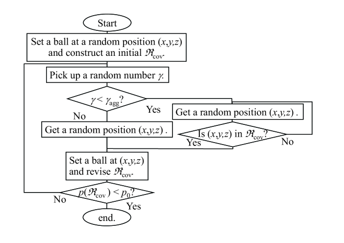
Figure 1: The flowchart of the agglomeration configuration algorithm.

We illustrate our algorithm by a flowchart in Figure 1. As an initial state, the configuration ${\mathfrak{R}}_{0}$ has no particle. As the first step, for a uniform random position $(x,y,z)\in{\mathcal{B}}$ we set a particle $B_{x,y,z}$ whose center is $(x,y,z)$ and the radius is $\rho$, i.e., ${\mathfrak{R}}_{1}:=B_{x,y,z}$.

Let us consider $n$-step. We take a position $(x,y,z)$ at uniform random in ${\mathcal{B}}$, and another random parameter $\gamma$ at uniform random in $[0,1]$. If the random parameter $\gamma$ is greater than $\gamma_{\rm{agg}}$, we employ the position $(x,y,z)$ as the center of a particle and ${\mathfrak{R}}_{n+1}:={\mathfrak{R}}_{n}\bigcup B_{x,y,z}$. It is noted that we allow the particles to overlap each other.

When the random parameter $\gamma$ is given as $\gamma\leq\gamma_{\rm{agg}}$, we first check whether the ball whose center is the position $(x,y,z)$ is connected with the previous configuration ${\mathfrak{R}}_{n}$ or not. If it is connected with the configuration ${\mathfrak{R}}_{n}$, or ${\mathfrak{R}}_{n}\bigcap B_{x,y,z}\neq\emptyset$, we employ the position and add the particle into the configuration ${\mathfrak{R}}_{n}$, or ${\mathfrak{R}}_{n+1}:={\mathfrak{R}}_{n}\bigcup B_{x,y,z}$.

If not, i.e., ${\mathfrak{R}}_{n}\bigcap B_{x,y,z}=\emptyset$, we abandon the position and go on to take another uniformly random position $(x,y,z)$ in ${\mathcal{B}}$ until we find the position which supplies a connected particle $B_{x,y,z}$ with ${\mathfrak{R}}_{n}$.

In other words, if we take $\gamma$ which is smaller than $\gamma_{\rm{agg}}$, the added particle must be connected with the previous configuration ${\mathfrak{R}}_{n}$. Thus, $\gamma_{\rm{agg}}$ stands for the agglomeration of the particle system.

By monitoring the total volume fraction which is a function of ${\mathfrak{R}}_{n}$ and is denoted by ${\rm{vol}}({\mathfrak{R}}_{n})$, we continue to put the particles as long as ${\rm{vol}}({\mathfrak{R}}_{n})\leq p$ for a given volume fraction $p$. We find the step $n(p)$ such that ${\rm{vol}}({\mathfrak{R}}_{n(p)-1})\leq p$ and ${\rm{vol}}({\mathfrak{R}}_{n(p)})>p$. Since the difference between ${\rm{vol}}({\mathfrak{R}}_{n(p)-1})$ and ${\rm{vol}}({\mathfrak{R}}_{n(p)})$ is at most $0.9\times 10^{-4}$ for the employed parameters, we regard ${\rm{vol}}({\mathfrak{R}}_{n(p)})$ as the volume fraction $p$ itself hereafter under this accuracy.

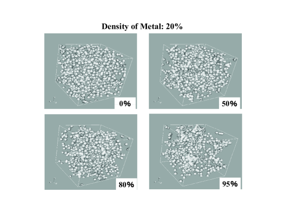
Figure 2: The agglomeration parameters: Random particle systems with the agglomeration parameter $\gamma_{\rm{agg}}$ $=0.0,0.5,0.8$ and $0.95$ for (a), (b), (c) and (d) respectively.

As illustrated in Figure 2, the uniform random configuration is realized as the case $\gamma_{\rm{agg}}=0$, and the agglomeration configurations are given with our agglomeration parameter $\gamma_{\rm{agg}}>0$. We regard ACPM of the case $\gamma_{\rm{agg}}=0$ as the ordinary CPM for balls with the same radius [11, 17] and thus we simply call it CPM hereafter.

In our algorithm, $B_{x,y,z}$ in ${\mathfrak{R}}_{n}$ is determined only by the previous configuration ${\mathfrak{R}}_{n-1}$ as a conditional probabilistic problem like $\Pr(B_{x,y,z}|{\mathfrak{R}}_{n-1})$. Since the configuration ${\mathfrak{R}}_{n-1}$ memorizes $n-1$ past outcomes $(B_{x_{i},y_{i},z_{i}})_{i=1,2,\ldots,n-1}$, it cannot be regarded as a Markov chain for $\gamma_{\rm{agg}}\neq 0$ [23, 24]. However we have a natural hierarchical properties ${\mathfrak{R}}_{n}\subset{\mathfrak{R}}_{n+1}$ as a sequential events governed by conditional probabilities for $\gamma_{\rm{agg}}\neq 0$ case and by the independent probability for the vanishing $\gamma_{\rm{agg}}$ case. Since we use the pseudo-randomness to simulate the random configuration ${\mathfrak{R}}_{n(p)}$ for given $p$ and $\gamma_{\rm{agg}}$, the configuration ${\mathfrak{R}}_{n(p)}$ depends upon the seed $i_{s}$ of the pseudo-randomness which we choose. We let it be denoted by ${\mathfrak{R}}_{\gamma_{\rm{agg}},p,i_{s}}$. In other words, for a certain seed $i_{s}$ of the pseudo-randomness, we handle the set of the configurations $\{{\mathfrak{R}}_{\gamma_{\rm{agg}},p,i_{s}}\ |\ p\in[0,1]\}$ as the sequence of the outcomes of the conditional probabilistic problems. Due to the hierarchical properties, ${\mathfrak{R}}_{\gamma_{\rm{agg}},p,i_{s}}$ is the events under the prior conditions ${\mathfrak{R}}_{\gamma_{\rm{agg}},p^{\prime},i_{s}}$ for $p^{\prime}<p$, and the configuration ${\mathfrak{R}}_{\gamma_{\rm{agg}},p,i_{s}}$ of a volume fraction $p$ naturally contains a configuration ${\mathfrak{R}}_{\gamma_{\rm{agg}},p^{\prime},i_{s}}$ for $p^{\prime}<p$, i.e., ${\mathfrak{R}}_{\gamma_{\rm{agg}},p^{\prime},i_{s}}\varsubsetneqq{\mathfrak{R}}_{\gamma_{\rm{agg}},p,i_{s}}$. Hence the elements in the set of the configurations $\{{\mathfrak{R}}_{\gamma_{\rm{agg}},p,i_{s}}\ |\ p\in[0,1]\}$ keeping the same seed $i_{s}$ are relevant and have the (total ordered) hierarchical structure,

$${\mathfrak{R}}_{\gamma_{\rm{agg}},0,i_{s}}\varsubsetneqq{\mathfrak{R}}_{\gamma_{\rm{agg}},p_{1},i_{s}}\varsubsetneqq{\mathfrak{R}}_{\gamma_{\rm{agg}},p_{2},i_{s}}\varsubsetneqq\cdots\varsubsetneqq{\mathfrak{R}}_{\gamma_{\rm{agg}},1,i_{s}},$$ (2)

for $0<p_{1}<p_{2}<\cdots<1$. As we compute their total conductivities and the conductivity curve $(\sigma_{\mathrm{total}}($ $\gamma_{\rm{agg}},p,i_{s}))_{p\in[0,1]}$ of (1) in the following section, it is obvious that the curve $(\sigma_{\mathrm{total}}($ $\gamma_{\rm{agg}},p,i_{s}))_{p\in[0,1]}$ is a well-defined function over the path $({\mathfrak{R}}_{\gamma_{\rm{agg}},p,i_{s}})_{p\in[0,1]}$ in a measure space for a sequence of the conditional probabilistic events [23, 24]; for fixing $\gamma_{\rm{agg}}$, the curve $(\sigma_{\mathrm{total}}($ $\gamma_{\rm{agg}},p,i_{s}))_{p\in[0,1]}$ corresponds to $({\mathfrak{R}}_{\gamma_{\rm{agg}},p,i_{s}})_{p\in[0,1]}$ for each $i_{s}$. In other words, we can treat the statistical properties, such as variance and average, of the conductivity curves in our method following the arguments of the infinite probability fields in [24, Chap II].

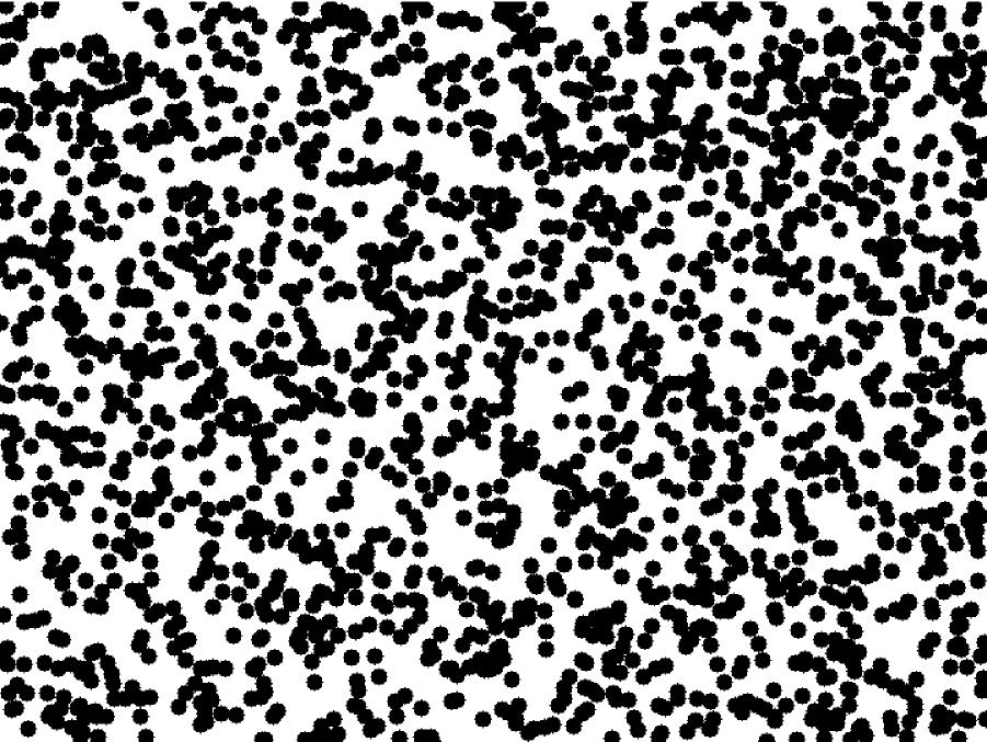
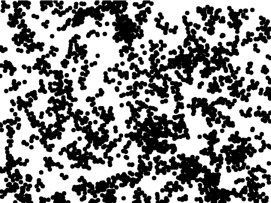
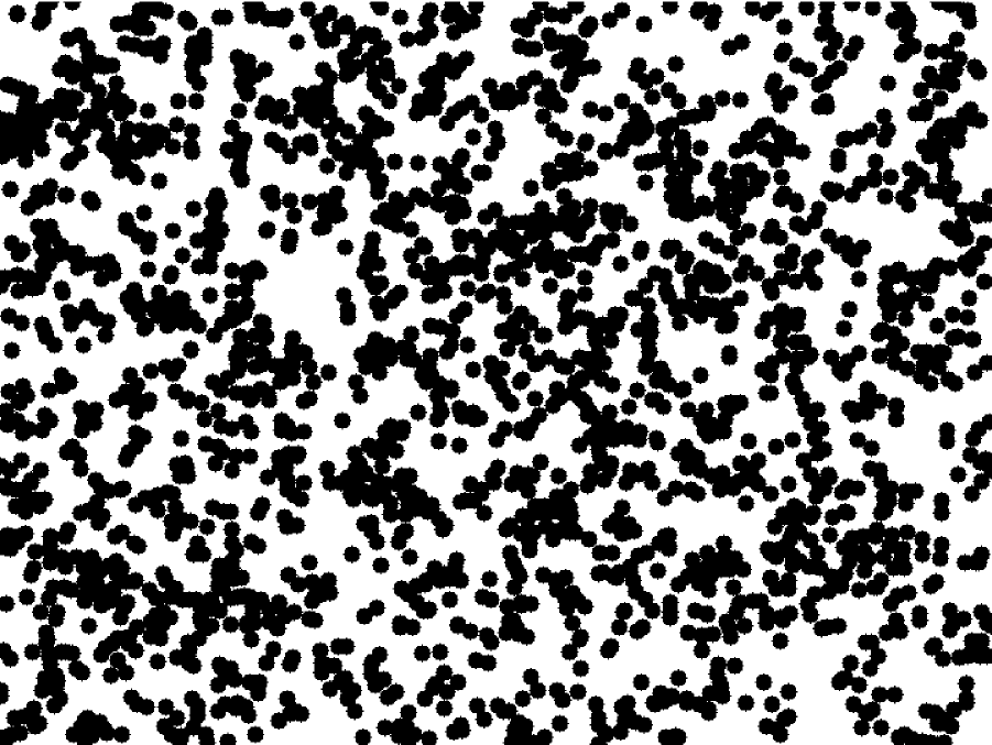
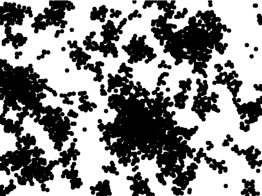
(a) (c) (b) (d)

Figure 3: The agglomeration parameters: Two-dimensional random particle system with the agglomeration parameter $\gamma_{\rm{agg}}$ $=0.0,0.5,0.8$ and $0.95$ for (a), (b), (c), and (d) respectively. The radius of the particle is six meshes, the width and height of the images are 720 and 540 meshes respectively, and the area fraction of the particles is 0.45.

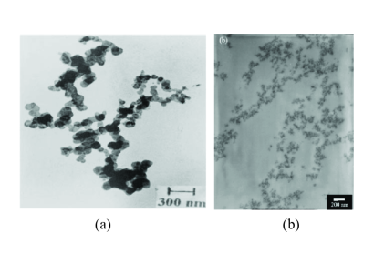
Figure 4: TEM micrograms of (a) polyacrylonitrile nanocomposite of acetylene black particles in Ref. [8] and (b) epoxy nanocomposites containing silicate oxide particles in Ref. [25].

In order to illustrate this algorithm, we will show two dimensional case. In a very similar way to the three-dimensional case, we have two dimensional agglomeration configurations which are given in Figure 3. Figure 4 exhibits the transmission electron micrograph (TEM) of the real agglomerated clusters in Refs. [8] and [25]. Ref. [8] is of the composite of polyacrylonitrile with acetylene black particles, and Ref. [25] shows the epoxy nanocomposites with silicate oxide particles. These configurations in Figure 3 might simulate some agglomeration states in Figure 4. Even though it is difficult to visualize the three dimensional cases well, it is expected that our algorithm generates the similar agglomerate configurations in Figure 2.

If we employ other more physical treatments for agglomeration such as [9, 10], it is difficult to find a parameter which directly represents the agglomeration, and is also hard to have a natural hierarchical property such as (2). In other words, we cannot basically define the conductivity curve as a function over a path in a measure space though of course, a single conductivity curve over $p\in[0,1]$ can be defined as a fitting curve for total conductivities to configurations. It means that our method has an advantage as a mathematical model.

2.2 Computation of the conductivity in ACPMs

To apply FDM [2] to the computation of the conductivity in ACPM, we use a $N_{x}\times N_{y}\times N_{z}$ lattice denoted by ${\mathcal{L}}$ to represent the box-region ${\mathcal{B}}$ by the integers $N_{x}$, $N_{y}$ and $N_{z}$. In this article, we mainly assume that $N_{x}=N_{y}=N_{z}=216$ and the radius of the particle $\rho=1$ corresponds to six meshes. It means that the ratio between the volumes of ${\mathcal{B}}$ and a particle is about $1.1\times 10^{4}$ and the size of ${\mathcal{B}}=[0,L]^{3}$ is given as $L\approx 36$.

Further we set the conductivity distribution $\sigma(x,y,z)$ which consists of the conductive particles and the insulator as a background in the box-region ${\mathcal{B}}$ as in Figure 2. We put the local conductivity $\sigma_{\rm{mat}}=1$ inside of each ${\mathfrak{R}}_{\gamma_{\rm{agg}},p,i_{s}}$. As the insulator, we set the infinitesimal conductivity $\sigma_{{\rm{inf}}}=10^{-4}$ within background. In other words, we handle binary materials with largely different local conductivities $\sigma_{\rm{mat}}$ and $\sigma_{\rm{inf}}$.

In order to compute the total conductivity, we set the voltage $\phi=\phi_{0}=1$ and $\phi=0$ on the upper and the lower faces, i.e., $[0,x_{0}]\times[0,y_{0}]\times\{z_{0}\}$ and $[0,x_{0}]\times[0,y_{0}]\times\{0\}$ respectively as the boundary condition corresponding to the electrodes. As the side boundary condition, we used the natural boundary for each $yz$-face and each $xz$-face. In other words, at the side boundaries, we imposed that current normal to each face vanished.

Following our algorithm of FDM as mentioned in detail in Ref. [1], we numerically solved the generalized Laplace equation over the region,

$$\nabla\cdot\sigma\nabla\phi=0,$$ (3)

for the conductivity distribution $\sigma(x,y,z)$ for each ${\mathfrak{R}}_{\gamma_{\rm{agg}},p,i_{s}}$ to obtain the potential distribution $\phi(x,y,z)$. By numerically solving (3), we obtained the total conductivity $\sigma_{\mathrm{total}}$ of the system after we integrated the current $\sigma\nabla\phi$ over a $xy$-plane. Since $\sigma_{\mathrm{total}}$ is determined for each ${\mathfrak{R}}_{\gamma_{\rm{agg}},p,i_{s}}$, $\sigma_{\mathrm{total}}$ is a function of the volume fraction $p$, the agglomeration parameter $\gamma_{\rm{agg}}$ and the seed $i_{s}$ of the pseudo-randomness. We denote it by $\sigma_{\mathrm{total}}(p,\gamma_{\rm{agg}},i_{s})$ explicitly or simply $\sigma_{\mathrm{total}}(p)$.

As mentioned in Introduction, the conductivity curve $\sigma_{\mathrm{total}}(p)$ $(p\in[0,1])$ is expressed by

$$\sigma_{\mathrm{total}}(p)=\left\{\begin{array}[]{ll}\frac{(p-p_{c})^{t}}{(1.0-p_{c})^{t}},&\mbox{for}\ p\in[p_{c},1],\\ 0&\mbox{otherwise},\\ \end{array}\right.$$ (4)

where $p_{c}$ is the threshold and ${t}$ is the critical exponent, or merely exponent. As mentioned in Subsection 2.1, the conductivity curve is a function over a path $({\mathfrak{R}}_{\gamma_{\rm{agg}},p,i_{s}})_{p\in[0,1]}$ in the measure space, which is characterized by the agglomeration parameter $\gamma_{\rm{agg}}$ and the seed $i_{s}$ of the pseudo-randomness. Thus the threshold $p_{c}$ and the exponent ${t}$ are naturally determined for the individual curve and can be regarded as functions of the agglomeration parameter $\gamma_{\rm{agg}}$ and the seed $i_{s}$, which we sometimes express as $p_{c}(\gamma_{\rm{agg}},i_{s})$ and ${t}(\gamma_{\rm{agg}},i_{s})$.

Therefore we evaluated the threshold $p_{c}(\gamma_{\rm{agg}},i_{s})$ and the exponent ${t}(\gamma_{\rm{agg}},i_{s})$ as the fitting parameters so that each average of the square error from the curve is the smallest, by monitoring the square root of the average of the square error. The square root of the average of the square error is denoted by $\delta\sigma_{\mathrm{total}}$ $\equiv\delta\sigma_{\mathrm{total}}(\gamma_{\rm{agg}},i_{s})$.

3 Results

For each seed $i_{s}$ of the pseudo-randomness, the total conductivities $\sigma_{\mathrm{total}}(p,$ $\gamma_{\rm{agg}},i_{s})$ are obtained over $\{{\mathfrak{R}}_{\gamma_{\rm{agg}},p,i_{s}}\ |\ p\in[0,1]\}$ with the hierarchical structure (2) as a conditional probabilistic problem. In other words, for each $i_{s}$, we obtained the conductivity curve $(\sigma_{\mathrm{total}}(p,\gamma_{\rm{agg}},i_{s}))_{p\in[0,1]}$ over the $({\mathfrak{R}}_{\gamma_{\rm{agg}},p,i_{s}})_{p\in[0,1]}$ as a measurable function even with the non-vanishing $\gamma_{\rm{agg}}$; if need be, we can justify it using the arguments of the infinite probability fields in [24, Chap II].

(a) (b)

Figure 5: The conductivity curves for agglomeration parameters $\gamma_{\rm{agg}}=0.0,0.5,0.8$ and $0.95$ of the seed $i_{s}=1$ of the pseudo-randomness: (a) is of the linear scale and (b) is of the logarithm scale.

Figure 5 illustrates the conductivity curves for the seed $i_{s}=1$ of the pseudo-randomness. Figure 5(b) shows that we handled the binary conductive materials. The dependence of agglomeration parameters on the conductivity curves for seed $i_{s}$ of the pseudo-randomness in Figures 6 and 7.

Figure 6: The conductivity curves for agglomeration parameters $\gamma_{\rm{agg}}=0.0,0.5,0.8$ and $0.95$ of the seed $i_{s}=1,2,\dots,12$ of the pseudo-randomness.

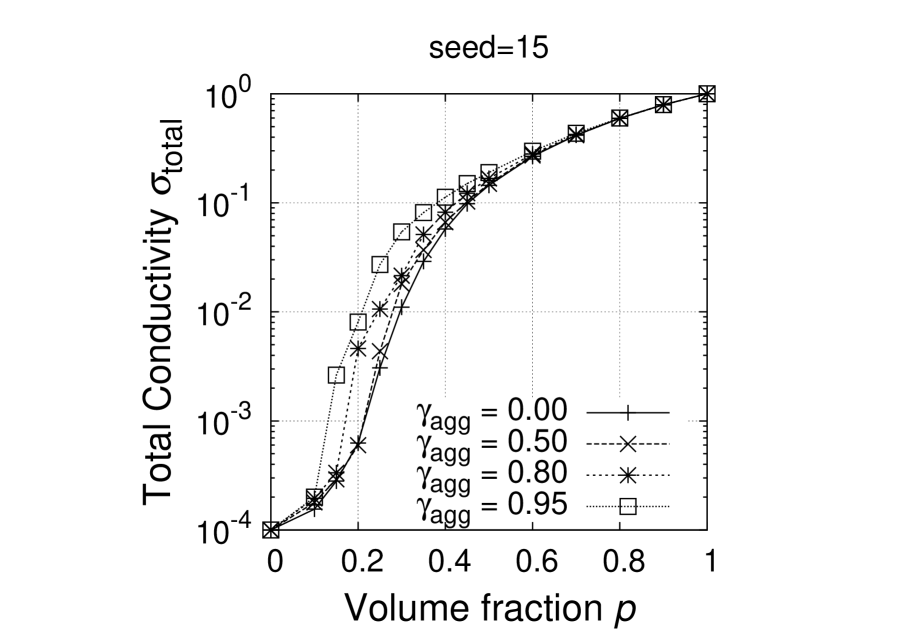
Figure 7: The conductivity curves for agglomeration parameters $\gamma_{\rm{agg}}=0.0,0.5,0.8$ and $0.95$ of the seed $i_{s}=13,14,\dots,20$ of the pseudo-randomness.

When $p=0$, the total conductivity $\sigma_{\mathrm{total}}$ is equal to $\sigma_{\rm{inf}}$ which stands for the insulator and is negligible if we dealt with $\sigma_{\mathrm{total}}$ linearly as shown in Figure 5(a). By using the least square error fitting method, we evaluated the threshold $p_{c}(\gamma_{\rm{agg}},i_{s})$ and the exponent ${t}(\gamma_{\rm{agg}},i_{s})$ from the curve. In the evaluation, we used the linear scale of $\sigma_{\mathrm{total}}$ or the curves in Figure 5(a). Figure 8 shows the fitting errors $\delta\sigma_{\mathrm{total}}$ v.s. the seed $i_{s}$ of the pseudo-randomness; $\delta\sigma_{\mathrm{total}}$ is the average of the squares of the deviations from the curve (4) over the fitting points for each $\gamma_{\rm{agg}}$ and $i_{s}$; the fitting points are $0.1$, $0.15$, $0.2$, $0.25$, $0.3$, $0.35$, $0.4$, $0.45$, $0.5$, $0.6$, $0.7$, $0.8$, and $0.9$. We computed thirty curves for each case, $\gamma_{\rm{agg}}=0.0$, $0.5$, $0.8$ and $0.95$. The deviations $\delta\sigma_{\mathrm{total}}$ are not large even for non-vanishing $\gamma_{\rm{agg}}$ compared with $\sigma_{\rm{mat}}=1$. The distribution of $\delta\sigma_{\mathrm{total}}$ shows that the larger $\gamma_{\rm{agg}}$ is, the larger the values are. Its maximum is $\delta\sigma_{{\mathrm{total}},\mathrm{max}}\leq 0.0084$ for $\gamma_{\rm{agg}}=0.95$, but the average $\overline{\delta\sigma_{\mathrm{total}}}$ is less than 0.0048; the values of $(\gamma_{\rm{agg}},\overline{\delta\sigma_{\mathrm{total}}})$ are given as $(0.0,0.0035)$, $(0.5,0.0043)$, $(0.8,0.0047)$ and $(0.95,0.0048)$.

Figure 8: The fitting errors $\delta\sigma_{\mathrm{total}}$ v.s. the seed $i_{s}$ of the pseudo-randomness for $\gamma_{\rm{agg}}=0.0,0.5,0.8$ and $0.95$.

It means that the thresholds $p_{c}$ and the exponents ${t}$ represent the conductivity curves well in our computations. In fact since we have

$$\frac{\partial\sigma_{\mathrm{total}}(p)}{\partial p_{c}}=-\sigma_{\mathrm{total}}(p)\frac{1-p}{(1-p_{c})(p-p_{c})}t,\quad\frac{\partial\sigma_{\mathrm{total}}(p)}{\partial t}=\sigma_{\mathrm{total}}(p)\log\frac{p-p_{c}}{1-p_{c}},$$

the accuracies $\delta_{\sigma}p$ and $\delta_{\sigma}t$ of $p_{c}$ and $t$, could be estimated using $\delta\sigma_{\mathrm{total}}$;

$$\delta_{\sigma}p=\left|\left(\frac{\partial\sigma_{\mathrm{total}}}{\partial p_{c}}\right)^{-1}\right|\overline{\delta\sigma_{\mathrm{total}}},\quad\delta_{\sigma}t=\left|\left(\frac{\partial\sigma_{\mathrm{total}}}{\partial t}\right)^{-1}\right|\overline{\delta\sigma_{\mathrm{total}}}.$$

For example, around $p\approx 0.5$ $(\sigma_{\mathrm{total}}\approx 0.2)$, they are evaluated as $\delta_{\sigma}p\approx\overline{\delta\sigma_{\mathrm{total}}}\approx 0.005$ and $\delta_{\sigma}t\approx 4.3\overline{\delta\sigma_{\mathrm{total}}}\approx 0.022$ by setting $p_{c}\sim 0.27$, $t\sim 1.63$ as shown below.

As the case $\gamma_{\rm{agg}}=0$, our computational results are $p_{c}=0.273\pm 0.012$ and ${t}=1.628\pm 0.036$. It should be noted that these computational results are obtained by FDM method with finite lattice. As the previous article, we showed a finite size effect of the lattice by using an extrapolation scheme of a lattice-size dependence of $p_{c}$ and ${t}$, these computational results $p_{c}=0.273\pm 0.012$ and ${t}=1.628\pm 0.036$ are on the extrapolation line in Ref. [1]; The extrapolated values as shown in the previous article [1] are $p_{c}^{ex}=0.296\pm 0.013$ and ${{t}}^{ex}=1.580\pm 0.042$, which agree with $p_{c}=0.289573\pm 0.000002$ in Ref. [28] and ${t}=1.6\pm 0.1$ in Refs. [26] and [27]. Hence our computational scheme is consistent with these results [1, 26, 27, 28].

In this article, since we focus on the difference of the conductive properties among several $\gamma_{\rm{agg}}$’s, we basically fix the lattice-size and investigate the conductivities in the finite region ${\mathcal{B}}$ without any corrections for the finite-lattice effects.

(a) (b)

Figure 9: The agglomeration dependence of the thresholds (a) and critical exponents (b). The filled circle corresponds to each computation for a seed of the pseudo-randomness and the dotted line shows the average.

The dependencies of exponents and thresholds upon the agglomeration parameter $\gamma_{\rm{agg}}$ are illustrated in Figure 9 and Table 1. Figure 9 shows that the agglomeration parameter $\gamma_{\rm{agg}}$ has large effects on the conductivity over ACPM beyond the accuracies $\delta_{\sigma}p_{c}\approx 0.005$ and $\delta_{\sigma}{t}\approx 0.022$. The larger the agglomeration parameter $\gamma_{\rm{agg}}$ is, the more largely the threshold and the exponent depend on the seed $i_{s}$. It means that the variance is enhanced by the agglomeration parameter $\gamma_{\rm{agg}}$.

Furthermore the larger the agglomeration parameter $\gamma_{\rm{agg}}$ is, the smaller the trend of the threshold is and the larger that of the exponent is. As shown in Table 1, the larger the agglomeration parameter $\gamma_{\rm{agg}}$ becomes, the smaller the average of the thresholds $\overline{p_{c}}(\gamma_{\rm{agg}})$ is and the larger the average of the exponent $\overline{t}(\gamma_{\rm{agg}})$ is.

Table 1: The $\gamma_{\rm{agg}}$ dependence of the threshold and the exponent.

	Threshold			Exponent
$\gamma_{\rm{agg}}$	Average	Maximum	Minimum	Average	Maximum	Minimum
0.0	0.273	0.284	0.261	1.628	1.661	1.588
0.5	0.250	0.283	0.231	1.689	1.758	1.597
0.8	0.224	0.324	0.159	1.772	1.951	1.506
0.95	0.202	0.276	0.047	1.809	2.214	1.523

Figures 6 and 7 show that the dependence of agglomeration parameters $\gamma_{\rm{agg}}$ on the conductivity curves are enhanced under the threshold $p_{c}$ for the logarithm scale. Under the percolation threshold $p_{c}$, our computation can read the computation of dielectric behavior on a random configuration of metal particles in the dielectric matter, which was reported in Refs. [29] and [30] if we consider the conductivity as the dielectric constant. Physically speaking, the behavior is related to the electric breakdown. Though the differences $p<p_{c}$ have negligible effects on the estimations of the conductivity curves (5) due to the fitting method for the linear scaling, they might be crucial for the dielectric behavior.

4 Discussion on the agglomeration effects

We now consider the reason why the agglomeration has the effects on the conductivity in our ACPM.

We have dealt with the percolation phenomena on a finite region ${\mathcal{B}}$ whereas it is well-known that the conductivity has dependence on the size of region as in Chapter 5.1 in Ref. [11]. We naturally have the characteristics length $r_{c}$ induced from the size of the particles or the radius of the particle $\rho$; for vanishing $\gamma_{\rm{agg}}$, i.e., $r_{c}(\gamma_{\rm{agg}}=0)=\rho$. Due to the finiteness of size $L$ of ${\mathcal{B}}$, the ratio $L/r_{c}$ has an effect on the conductivity; at $\gamma_{\rm{agg}}=0$, we have that $L/r_{c}\approx 36$. For non-vanishing agglomeration parameter $\gamma_{\rm{agg}}\neq 0$, it is expected that the characteristic length $r_{c}$ is larger than that of CPMs ($\gamma_{\rm{agg}}=0$) due to the agglomeration, i.e., $r_{c}(\gamma_{\rm{agg}}\neq 0)>\rho$. Further by letting $\xi=\xi(p,\gamma_{\rm{agg}})$ be the correlation length which represents the percolation phenomenon, we should compare the size of region $L$, the correlation length $\xi$ and the characteristic length $r_{c}$. According to Chapter 5.1 in Ref. [11], the total conductivity behaves like

$$\sigma_{\mathrm{total}}(p,\gamma_{\rm{agg}})\propto\left\{\begin{array}[]{ll}(\xi/r_{c})^{-\mu},&\mbox{for}\ L/r_{c}\gg(\xi/r_{c}),\\ (L/r_{c})^{-\mu},&\mbox{for}\ L/r_{c}\ll(\xi/r_{c}),\\ \end{array}\right.$$ (5)

where $\mu$ is the non-negative parameter (73a) in Ref. [11]. Since it is known that $\xi$ diverges at the critical point $p_{c}$ and in every numerical estimation we handle only a finite region, the formula (5) means that every numerical estimation gives higher conductivity in the vicinity of the point $p_{c}$ than that of an infinite region apart from the variances.

Though the percolation theory is basically concerned with conductivity curve in the infinite region, we concern ourselves about the size effect of the real materials. Further in Ref. [1], we have showed that the shape effect has crucial effects on the conductivity curves. Thus we will consider the geometrical properties of agglomerated clusters.

4.1 The geometrical features in ACPM

Let us consider the size and the shape of the agglomerated clusters which depend on the agglomeration parameter $\gamma_{\rm{agg}}$.

4.1.1 The characteristic length $r_{c}$ in ACPM at $p=0.1$

First we consider the size effect and give an estimation on the characteristic length $r_{c}$ for non-vanishing $\gamma_{\rm{agg}}$. Since it is difficult to estimate it, we compute the difference among the size of the isolated agglomerated clusters at a lower volume fraction $p$ than $p_{c}$. In other words, we compute statistical behavior of the percolation clusters, or the connected particles, at $p=0.1$.

When the agglomeration parameter $\gamma_{\rm{agg}}$ becomes large, it is expected that the size of the percolation cluster becomes larger than one of the uniform randomness or the case ($\gamma_{\rm{agg}}=0$). The size of the percolation cluster is associated with the correlation length $\xi(p,\gamma_{\rm{agg}})$ in (5).

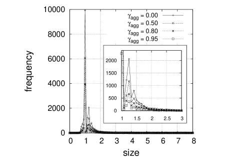
Figure 10: The histogram of size $\rho_{\rm{clst}}$ of percolation cluster for each agglomeration parameter $\gamma_{\rm{agg}}$ at $p=0.1$.

In order to evaluate the effect of the size, we consider effective radius $\rho_{\rm{clst}}$ and maximum length $L_{\rm{max}}$ of each agglomerated clusters in ACPM, and the numbers $N_{\rm{agg}}$ of agglomerated clusters. Here the effective radius $\rho_{\rm{clst}}$ is defined such that $4\pi\rho_{\rm{clst}}^{3}/3$ is equal to the volume of the percolation cluster. First, we consider a histogram of the effective radius $\rho_{\rm{clst}}$. Figure 10 shows frequency of the effective radius $\rho_{\rm{clst}}$ at the volume fraction $p=0.1$ which is smaller than any thresholds $\overline{p_{c}}(\gamma_{\rm{agg}})$. Figure 10 means that the larger the agglomeration parameter $\gamma_{\rm{agg}}$ is, the larger the size of the cluster is.

Figure 10 shows the fact that the histogram has two peaks; the first peak at $\rho_{\rm{clst}}=\rho$ as the size of isolated particle, and the second peak around $\rho_{\rm{clst}}=\sqrt[3]{2}\approx 1.26\rho$ as the size of two particles. The probability of two slightly connected particles is larger than the probability of the state which has $\rho_{\rm{clst}}\in(\rho,\sqrt[3]{2}\rho)$ because of radial measure $\rho_{\rm{clst}}^{2}d\rho_{\rm{clst}}$ for the radius $\rho_{\rm{clst}}$ from the center of a particle. The percolation is determined by the largest cluster size but it should be statistically treated. We consider the right hand side of the second peak of the histograms. We fit the shape of the histogram over $\rho_{\rm{clst}}\in[1.3,8]$ by $h(\rho_{\rm{clst}})=A\exp(-(\rho_{\rm{clst}}-\rho)/\rho_{\rm{clst}}^{0})$ well using the least mean square error method, where $A$ and $\rho_{\rm{clst}}^{0}$ are fitting parameters. Then $\rho_{\rm{clst}}^{0}$ is given in Table 2. Here $\delta h$ is the square root of the average of the least mean square error.

Table 2: The $\rho_{\rm{clst}}$ dependence on the agglomeration parameter $\gamma_{\rm{agg}}$.

$\gamma_{\rm{agg}}$	0	0.5	0.8	0.95
$\rho_{\rm{clst}}^{0}/\rho$	0.315	0.458	0.476	0.522
$\delta h$	0.020	0.019	0.024	0.028

Table 2 shows that the agglomeration parameter $\gamma_{\rm{agg}}$ increases the size of the clusters at $p=0.1$. The characteristic length $r_{c}$ is directly relevant to the size of clusters $\rho_{\rm{clst}}^{0}$. Though it is difficult to evaluate the difference of the size of clusters $\rho_{\rm{clst}}^{0}$ and also $r_{c}$ at $p\geq p_{c}$, it is expected that it plays similar roles even for every $p\in[0,1]$.

Table 3: The $\overline{\rho_{\rm{clst}}}$, $\overline{L_{\rm{max}}}$, and $N_{\rm{agg}}$ of the agglomerated ($\rho_{\rm{clst}}>1.3$) particles dependence on the agglomeration parameter $\gamma_{\rm{agg}}$ at $p=0.1$.

$\gamma_{\rm{agg}}$	0	0.5	0.8	0.95
$\overline{\rho_{\rm{clst}}}$	1.572	1.800	1.978	2.200
$\overline{L_{\rm{max}}}/2$	2.803	3.310	3.668	4.009
$N_{\rm{agg}}$	2977	2725	1722	952

Further Table 3 shows the averages of the size $\overline{\rho_{\rm{clst}}}$ and the maximum distance $\overline{L_{\rm{max}}}$ of the percolation clusters which have $\rho_{\rm{clst}}>1.3\rho$, and their number $N_{\rm{agg}}$. The larger $\gamma_{\rm{agg}}$ is, the larger $\overline{L_{\rm{max}}}$ and $\overline{\rho_{\rm{clst}}}$ are, and the smaller $N_{\rm{agg}}$ is.

They mean that the larger $\gamma_{\rm{agg}}$ is, the smaller the ratio $L/r_{c}$ is. Hence it is expected that the larger $\gamma_{\rm{agg}}$ is, the larger the variance becomes.

4.1.2 The shape of the agglomerated cluster in ACPM

Here we consider the shape of the agglomerated cluster. In our algorithm which is shown in Figure 1, a new particle with $\gamma<\gamma_{\rm{agg}}$ must be connected with the particles which have been already placed. If the volume fraction is much less than the threshold, the connected (agglomerated) cluster which consists of $N$ particles could be regarded as an orbit of a random walk for discrete $N$ time step.

In fact, the size of the agglomerated cluster is proportional to the square root of $N$ as shown in Figure 11. Figure 11 displays the correlation between the $L_{\rm{max}}$ and $\sqrt{N}$ for $\gamma_{\rm{agg}}=0.0,0.5$. They are linearly relative. This coincides with the properties of the random walk due to the central limit theorem [23].

(a) (b)

Figure 11: The dependence of the $L_{\rm{max}}$ on the $\sqrt{N}$ for $\gamma_{\rm{agg}}=0.0,0.5$.

Figure 11 means that if we regard the agglomerated cluster as a cylinder, the radius around the center axis is proportional to $\sqrt[4]{N}$ since the volume should be proportional to $N$ but $L_{\rm{max}}\propto\sqrt{N}$. For a sufficiently large $N$, the agglomerated cluster might be regarded as a thin cylinder rather than a thick cylinder.

4.2 The agglomeration effect on conductivity in ACPM

In this section, we will investigate the behavior in Figure 9 as the agglomeration effect on conductivity in ACPM.

As shown above, when we fix ${\mathcal{B}}$, the larger $r_{c}(\gamma_{\rm{agg}})$ becomes, the smaller the effective size $L/r_{c}$ in (5) is regarded. It is expected that the total conductivity $\sigma_{\mathrm{total}}(p,\gamma_{\rm{agg}},i_{s})$ strongly depends on the configuration ${\mathfrak{R}}_{\gamma_{\rm{agg}},p,i_{s}}$ since statistical average does depend upon the ratio $L/r_{c}$ which is not sufficiently large for $\gamma_{\rm{agg}}>0$. As shown in Figure 9, it means that the larger $\gamma_{\rm{agg}}$ is, the more largely the threshold $p_{c}(\gamma_{\rm{agg}}\neq 0,i_{s})$ and the exponent ${t}(\gamma_{\rm{agg}}\neq 0,i_{s})$ depend on the seed $i_{s}$. Thus we consider the size effect first.

4.2.1 The size effect on conductivity in CPM

In this subsection we consider the size effect on conductivity in CPM or the case $\gamma_{\rm{agg}}=0$ by changing the radius $\rho$ directly.

We computed the threshold $p_{c}$ and the exponent ${t}$ for the different radius $\rho(>1)$ by fixing the size of ${\mathcal{B}}$. (From the numerical viewpoint, we performed the similar computations of $\gamma_{\rm{agg}}=0$ for small $N_{x}=N_{y}=N_{z}$ by fixing the mesh of $\rho$. It corresponds to the variation of the radius $\rho$ of the particles for fixing ${\mathcal{B}}$ relatively.)

(a) (b)

Figure 12: Thresholds (a) and critical exponents (b) vs radius of particles in the same ${\mathcal{B}}$. The filled circle corresponds to each computation for a seed and the dotted line is their average.

Figure 13: The conductivity curves for the radius $\rho=1.0,1.35,2.0,2.7,$ and $3.86$ in the same ${\mathcal{B}}$ for the seed $i_{s}=1,2,\dots,9$ of the pseudo-randomness.

Figure 13 illustrates the dependence of the particle radius $\rho$ on the conductivity curves for the logarithm scale for nine cases, though we computed thirty cases for each $\rho$. Figure 12 and Table 4 give the dependence of the threshold and the exponent on the size of particles for the same ${\mathcal{B}}$. Figure 12 shows that the (relatively) larger the radius $\rho$ is, the larger the dispersions of the threshold $p_{c}$ and the exponent ${t}$ are. This property is similar to Figure 9. However the dispersions of both threshold and exponent in Figure 12 look symmetric with respect to their averages whereas the dispersions in Figure 9 show asymmetry.

(a) (b)

Figure 14: Critical exponents vs thresholds (a) for various $\rho$ with $\gamma_{\rm{agg}}=0.0$, and (b) for various $\gamma_{\rm{agg}}$ with $\rho=1$.

The equation (5) is evaluated from the statistical viewpoint. There is no difference among $\rho$’s if ${\mathcal{B}}$ has infinite region. Since ${\mathcal{B}}$ has a finite size, for large $\rho$, we don’t have so sufficiently many particles in ${\mathcal{B}}$ that its statistical average works well. Hence the deviation is enhanced. In other words, the dependence of the conductivity curve (4) on the seed $i_{s}$ of the pseudo-randomness is larger than that of $\rho=1$ as in Figure 12.

Since (5) means that the finiteness of ${\mathcal{B}}$ makes the threshold $p_{c}$ small statistically, the trend of the statistical average of the threshold shows that the larger the size $\rho$ in CPM is, the smaller the threshold $\overline{p_{c}}(\rho)$ is as shown in Table 4 and Figure 12 (a). Here, $\overline{p_{c}}(\rho)$ stands for the statistical average of the $p_{c}(\rho,i_{s})$ over the seed $i_{s}$ of the pseudo-randomness. This property of the threshold is also similar to Figure 9 (a), though the dependence of the exponents in Figure 12 (b) is quite different from Figure 9 (b).

When the individual total conductivity $\sigma_{\mathrm{total}}(p,\rho,i_{s})$ has smaller $p_{c}(\rho,i_{s})$ than $\overline{p_{c}}(\rho)$, the non-vanishing $\sigma_{\mathrm{total}}(p,\rho,i_{s})$ at $p\in(p_{c}(\rho,i_{s}),\overline{p_{c}}(\rho))$, must increase weakly with respect to $p$. It means that the exponent ${t}(\rho,i_{s})$ becomes larger in the conductivity curve (4) than its average $\overline{{t}}$. It implies that the exponent ${t}(\rho,i_{s})$ and the threshold $p_{c}(\rho,i_{s})$ in CPMs of different $\rho$ and $i_{s}$ are correlative and that the smaller the thresholds $p_{c}(\rho,i_{s})$ are, the larger the exponents ${t}(\rho,i_{s})$ are. Particularly Figure 14(a) exhibits the correlation between the exponent $t$ and the threshold $p_{c}$ in CPMs.

Table 4: The $\rho$ dependence of the threshold and the exponent.

	Threshold			Exponent
$\rho$	Average	Maximum	Minimum	Average	Maximum	Minimum
1.0	0.273	0.284	0.261	1.628	1.661	1.588
1.35	0.269	0.291	0.246	1.620	1.711	1.530
2.0	0.274	0.305	0.232	1.572	1.742	1.457
2.7	0.260	0.324	0.192	1.581	1.836	1.340
3.86	0.242	0.345	0.152	1.568	1.873	1.253

4.2.2 The size effect on conductivity in ACPM

Following the above discussions, we consider the agglomeration effect on the conductivity in our ACPM.

Subsection 4.1 means that the larger the agglomeration parameter $\gamma_{\rm{agg}}$ is, the larger the size of the percolation clusters and characteristic length $r_{c}$ are and the smaller the effective size $L/r_{c}$ in (5) is. For the agglomeration parameter $\gamma_{\rm{agg}}$ deviated from $0$, ${\mathcal{B}}$ corresponds to a relatively smaller region than the uniform random case ($\gamma_{\rm{agg}}=0$). Subsection 4.2.1 means that due to the finite size effect, the dependence of the threshold and the exponent upon the seed of the pseudo-randomness, i.e., these variances are larger than the case of $\gamma_{\rm{agg}}=0$. In other words, the large deviation for non-vanishing $\gamma_{\rm{agg}}$ comes from the finiteness of ${\mathcal{B}}$ and the size of the agglomerated clusters.

The dependence of the particle radius $\rho$ on the conductivity curves for the logarithm scale is displayed in Figure 13. The variance of the curves look enhanced under the threshold $p_{c}$. The same behavior is observed in Figures 6 and 7; the dependence of the agglomeration parameter $\gamma_{\rm{agg}}$ on the conductivity curves. It means that they also show the relation between the size effect and the agglomeration effect, as we mentioned above. Since the smaller $p$ is, the smaller the number of the clusters is, these effects becomes evident for small $p$.

Since the agglomeration makes the size of the characteristic length $r_{c}$ larger than that of non-agglomeration state, it is expected that $\overline{p_{c}}(\gamma_{\rm{agg}})>\overline{p_{c}}(\gamma_{\rm{agg}}^{\prime})$ for $\gamma_{\rm{agg}}<\gamma_{\rm{agg}}^{\prime}$. Here, $\overline{p_{c}}(\gamma_{\rm{agg}})$ represents the statistical average of $p_{c}(\gamma_{\rm{agg}},i_{s})$’s as a function of $\gamma_{\rm{agg}}$. In fact, Figure 9 shows that $\overline{p_{c}}(\gamma_{\rm{agg}})>\overline{p_{c}}(\gamma_{\rm{agg}}^{\prime})$ for $\gamma_{\rm{agg}}<\gamma_{\rm{agg}}^{\prime}$.

When an individual $p_{c}(\gamma_{\rm{agg}},i_{s})$ becomes smaller than $\overline{p_{c}}(\gamma_{\rm{agg}})$ for a large $\gamma_{\rm{agg}}$, the non-vanishing total conductivity $\sigma_{\mathrm{total}}(p,\gamma_{\rm{agg}},i_{s})$ is very small at $p\in(p_{c}(\gamma_{\rm{agg}},i_{s}),\overline{p_{c}}(\gamma_{\rm{agg}}))$ and increases weakly with respect to $p$ there. It means that the exponent ${t}(\gamma_{\rm{agg}},i_{s})$ becomes large in the conductivity curve (4). Figure 14(b) illustrates the correlation between the exponent ${t}(\gamma_{\rm{agg}},i_{s})$ and the threshold $p_{c}(\gamma_{\rm{agg}},i_{s})$ in ACPMs, which means that the smaller the thresholds $p_{c}(\gamma_{\rm{agg}},i_{s})$ are, the larger the exponents ${t}(\gamma_{\rm{agg}},i_{s})$ are. These properties are the same as Figure 14(a).

However the range of Figure 14(b) quite differs from Figure 14(a). The variances in Figure 12 look symmetric with respect to their averages whereas those in Figure 9 are asymmetry. The larger $\gamma_{\rm{agg}}$ is, the smaller the average of thresholds $\overline{p_{c}}(\gamma_{\rm{agg}})$ is and the larger that of the exponents $\overline{{t}}(\gamma_{\rm{agg}})$ is. Thus the trend of Figure 9 could not be interpreted only by the size effect. The difference might be regarded as an shape effect of the agglomerated clusters.

In the previous work [1], we investigated the shape effect on the CPMs for spheroid. The thinner the spheroid (of oblate case) is, the smaller we have thresholds and the larger we obtain exponents, whereas the thicker the spheroid (of prolate case) is, the smaller the threshold and the exponent are[1, 19] . As mentioned in Ref. [1], the shape effect can be also interpreted as the broad distribution continuum percolation model (BDCPM). Since the spheroids with random orientation can be regarded as a distribution (of probability) of the local conductivity, CPMs for a shaped object, e.g., spheroid can be interpreted as BDCPM from view point of the probability theory. It means that such properties of CPMs of the spheroid can be applied to any shape problem in CPM including this case. The thinner the shape of particles (or clusters) is, the smaller the threshold is and the larger the exponent is.

As showed in Subsection 4.1.2, it could be regarded that the larger $\gamma_{\rm{agg}}$ is, the thinner the shape of the agglomerated cluster becomes. Hence the properties of the averaged values in Figure 9 could be interpreted as the shape effects. In other words, the tendency of the threshold and the exponent agrees with that of thin shape effects of the spheroids. With the arguments in Subsections 4.1.1 and 4.1.2, it means that the larger $\gamma_{\rm{agg}}$ is, the smaller the threshold is and the larger the exponent is. This property reproduces Figure 9 and Table 1.

4.2.3 The universal properties of conductivity in ACPM

The variances of the threshold in CPM are essentially the same as those in ACPM if the agglomeration parameter $\gamma_{\rm{agg}}$ reads the size $\rho$ appropriately. Though the dependence of the average of the exponents on $\gamma_{\rm{agg}}$ differs from the $\rho$ dependence, we consider that the difference might come from the fact that the agglomerated cluster has a thin shape as another geometrical effect.

Let us attempt an investigation of the universal properties of ACPMs or the behavior of ACPMs in the infinite region.

Figure 15 exhibits the dependence of the threshold and the exponent on the size of the system for the $\gamma_{\rm{agg}}=0.5$ case. In the computations of Figure 15, we used larger $N=N_{x}=N_{y}=N_{z}$ analyzed regions as $N=272$ and $N=344$. The relative particle sizes (the radii) are $\rho=0.79$ and $\rho=0.63$. Since these computations are harder than $N=216$, we computed only twenty curves for these additional cases respectively as shown in Figure 15 and Table 5.

(a) (b)

Figure 15: The dependence of the thresholds and exponents on the size of the system for ACPM with $\gamma_{\rm{agg}}=0.5$. The filled circle corresponds to a computation for each seed $i_{s}$ of the pseudo-randomness and the dotted line is their average.

Table 5: The $\rho$ dependence of the threshold and the exponent for the case $\gamma_{\rm{agg}}=0.5$.

	Threshold			Exponent
$\rho$	Average	Maximum	Minimum	Average	Maximum	Minimum
$1.00^{\dagger}$	0.250	0.283	0.231	1.689	1.758	1.597
$0.79^{*}$	0.251	0.269	0.234	1.702	1.746	1.653
$0.63^{*}$	0.253	0.266	0.243	1.714	1.744	1.676

$*$: twenty curves. $\dagger$ thirty curves.

Figure 15 and Table 5 show that the smaller the radius $\rho$ is, the smaller the variances are. This means that the variances come from the size effect. They also show that the asymptotic values of the thresholds $p_{c}$ and the exponents $t$ might differ from those of $\gamma_{\rm{agg}}=0.0$, and they might not approach to those of $\gamma_{\rm{agg}}=0.0$. We conjecture that the agglomeration, at least in the case of our algorithm of agglomeration, would have effects on the universal properties. If there is the effect, the difference is expected to come from the shape effect of the agglomerated clusters as argued above.

5 Summary

By employing the simple algorithm to simulate an agglomerated configuration of particles, which is controlled by the agglomeration parameter $\gamma_{\rm{agg}}\in[0,1]$, we numerically show how the thresholds $p_{c}$ and the exponent ${t}$ of the conductivity curve (4) depend upon the agglomerations as shown in Figure 9. Since our algorithm is given as a sequence of conditional probabilistic events (2), we can statistically investigate the conductivity curves as functions over the sequences. The larger the agglomeration parameter $\gamma_{\rm{agg}}$ is, the larger the variance is. Further the larger $\gamma_{\rm{agg}}$ is, the smaller the average of the thresholds is and the larger the average of the exponents is.

From Section 4, we conclude that the origin of these effects could be interpreted as the size effect mainly, because the agglomeration makes the percolation clusters larger than those of non-agglomerated case. Since for the finite region, the enlargement of the clusters makes the variances of the conductivity large, the size effect is crucial if the size of system is not large enough.

Subsidiarily it is expected that the shape of the agglomerated clusters also affect the conductivity. It means that the shape of the agglomerated clusters might have effects on the universal properties of the threshold and the exponents as we attempted an investigation in Subsection 4.2.3.

Due to the development of the technology, devices with small sizes and the small conductive nanoparticles are concerned. Small particles basically agglomerate much due to their surface energy. Then in the conductivity in the composite materials of the conductive nanoparticles, the agglomeration causes the variances of the conductivity and the difference of individual devices. Hence we believe that our results shed a new light on the applications of the percolation theory to such a real material system.

References

- [1] S. Matsutani, Y. Shimosako, and Y. Wang, Int. J. Mod. Phys. C 21 (2010) 709-729.
- [2] R. J. LeVeque, Finite Difference Methods for Ordinary and Partial Differential Equations: Steady-State and Time-Dependent Problems (Classics in Applied Mathematics), (Soc. for Industrial & Applied, 1955 republished in 2007).
- [3] M. H. Al-Saleh and U. Sundararaj, Eur. Polymer J. 44 (2008) 1931-1939
- [4] Y. Konishi and M. Cakmak, Polymer 47 (2006) 5371-5391.
- [5] H-H. Leea, K-S. Choua, and Z-W. Shih, Int. J. of Adhesion & Adhesives 25 (2005) 437-441.
- [6] Z. Ranjbar and S. Rastegar, Colloids and Surfaces A : Physicochem. Eng. Aspects 290 (2006) 186-193.
- [7] H.P. Wu, X.J. Wu, M.Y. Ge, G.Q. Zhang, Y.W. Wang and J.Z. Jiang , Composites Sci. and Tech. 67 (2007) 1116-1120.
- [8] A. Maity and M. Biswas, Polymer J., 36 (2004). 812-816.
- [9] I. Tail, G. I. Tardos, and M. I. Khan, Powder Tech. 110 (2000) 59-75
- [10] P. Kosinski, and A. Hoffmann, Chem. Eng. Sci. 65 (2010) 3231-3239
- [11] D. Stauffer and A Aharony, Introduction to percolation theory, revised second ed., (CRC Press, Boca Raton, 1991).
- [12] G. E. Pike and C. H. Seager, Phys. Rev. B 10 (1973) 1421-1434.
- [13] G. E. Pike and C. H. Seager, Phys. Rev. B 10 (1973) 1435-1446.
- [14] M. B. Isichenko, Rev. Mod. Phys. 64 961-1043.
- [15] P. M. Kogut and J. P. Straley, J. Phsy. C 12 (1979) 2151-2159.
- [16] I. Balberg, Phys. Rev. Lett 59 (1987) 1305-1308.
- [17] R. Meester and R Roy, Continuum Percolation, Cambridge Tracts in Mathematics 119, (Cambridge, Cambridge, 1996).
- [18] G. Grimmett, Percolation, second ed., (Springer, Berlin, 1999).
- [19] E. J. Garboczi, K. A. Snyder, J. F. Douglas and M. F. Thorpe, Phys. Rev. E 52 (1995) 819-828.
- [20] Y. B. Yi, Phys. Rev. E 74 (2006) 031112:1-6.
- [21] V. Myroshnychenko and C. Brosseau, J. Phys. D: Appl. Phys. 41 (2008) 095401, 8pp.
- [22] S. J. Li, Y. F. Wang, Y. X. Liu, and W. Sun, Int. J. Mod. Phys. C 20 (2009) 513-526.
- [23] W. Feller, An Introduction to probability theory and its applications, 3rd ed., (Wiley, New York, 1967).
- [24] A. N. Kolmogorov, Foundations of the theory of probability, 2nd ed., trans. by N. Morrison and A. T. Bharucha-Reid, (Chelsea Publ., New York, 1956).
- [25] C-C. Chu, J-J. Lin, C-R. Shiu and C-C. Kwan, Polymer J., 37 (2005). 239-245.
- [26] A. B. Harris and S. Kirkpatrick, Phys. Rev. B 16 (1977) 542-576.
- [27] I. Webman, J. Jortner, and M. H. Cohen, Phys. Rev. B 16 (1977) 2593-2596.
- [28] C. D. Lorenz, and R. M. Ziff, J. Chem. Phys. 114 (2001) 3659-3661
- [29] M. F. Gyure and P. D. Beale, Phys. Rev. B. 40 (1989) 9533-9540.
- [30] H. Stoyanov, D. Mc Carthy, M. Kollosche and G. Kofod, Appl. Phys. Lett. 94 (2009) 232905.