An infinite-period phase transition versus nucleation in a stochastic model of collective oscillations

Abstract

A lattice model of three-state stochastic phase-coupled oscillators has been shown by Wood et al. (2006 Phys. Rev. Lett. 96 145701) to exhibit a phase transition at a critical value of the coupling parameter, leading to stable global oscillations. We show that, in the complete graph version of the model, upon further increase in the coupling, the average frequency of collective oscillations decreases until an infinite-period (IP) phase transition occurs, at which point collective oscillations cease. Above this second critical point, a macroscopic fraction of the oscillators spend most of the time in one of the three states, yielding a prototypical nonequilibrium example (without an equilibrium counterpart) in which discrete rotational ($C_{3}$) symmetry is spontaneously broken, in the absence of any absorbing state. Simulation results and nucleation arguments strongly suggest that the IP phase transition does not occur on finite-dimensional lattices with short-range interactions.

1 Introduction

Models of coupled oscillators exhibit a surprising range of symmetry-breaking transitions to a globally synchronized state. In the paradigmatic Kuramoto model, for instance, oscillators with intrinsic frequencies $\omega_{i}$ coupled via their continuous phases $\theta_{i}$ can exhibit stable collective oscillations, with breaking of time translation symmetry [1, 2, 3, 4, 5]. When $\omega_{i}=0$, the Kuramoto model acquires an additional $\theta_{i}\to-\theta_{i}$ reflection symmetry, which can also be broken at the onset of synchronization, yielding surprising response properties [6].

Within the class of discrete-phase models, the paper-scissors-stone game is an example of a system with three absorbing states which can present either global oscillations or spontaneous breaking of discrete rotational ($C_{3}$) symmetry [7, 8, 9, 10, 11]. More recently, Wood, Van den Broeck, Kawai and Lindenberg proposed a family of models of phase-coupled three-state stochastic oscillators which can undergo a phase transition to a synchronized state [12, 13, 14, 15] for sufficiently strong coupling. From here on each of them is called Wood et al.’s cyclic model (WCM). Although the WCM also has $C_{3}$ symmetry, it has no absorbing state.

As noted previously [14], the first WCM [12] has an unusual behavior after the phase transition to a synchronized state. As the phase coupling is further increased, collective oscillations slow down while oscillators remain partially synchronized. Here we have a closer look at this phenomenon, in particular addressing whether or not there is a second phase transition with breaking of $C_{3}$ symmetry.

The paper is organized as follows. In section 2 we review the WCM and the essentials of the known transition to a synchronized phase. Our results regarding a putative second phase transition are described in section 3. We conclude in section 4.

Figure 1: Transition rates for an isolated unit.

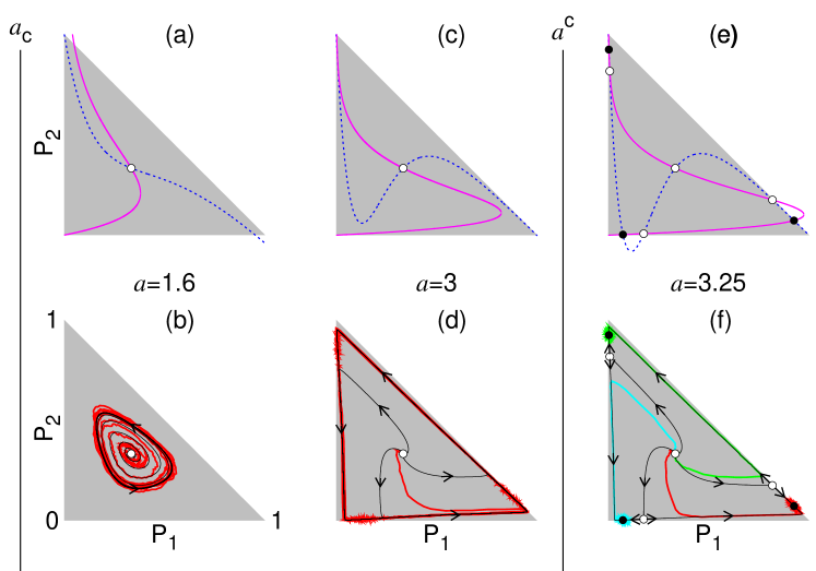
Figure 2: (Color online) Phase space $(P_{1},P_{2})$. Grey triangles correspond to the allowed region $0\leq P_{2}\leq 1-P_{1}$. $a$ increases from left to right. In the upper panels, dashed (solid) lines denote the nullclines $\dot{P}_{1}=0$ ($\dot{P}_{2}=0$). Lower panels show trajectories from complete graph simulations with $N=5000$ (thick lines) and solutions of the mean-field equations (thin lines with arrows). Panel (a) shows that $\vec{P}_{1/3}^{*}$ is the only fixed point in the system for $a=1.6>a_{c}$. (b) $\vec{P}_{1/3}^{*}$ is unstable, with trajectories converging to a stable limit cycle, which corresponds to sustained global oscillations (see also Fig. 3a). (c) For $a=3$, the nullclines approach one another in three additional positions, thereby creating three symmetric saddle-node ghosts. (d) The limit cycle is almost as large as the perimeter of the allowed region. Note the overcrowding of lines near the ghosts, with consequent anharmonicity in the time series (Fig. 3b). (e) For $a=3.25$ there are six additional fixed points which are born simultaneously in three saddle-node bifurcations at $a=a^{c}$. (f) In this case, if the system starts from the symmetric unstable fixed point $\vec{P}_{1/3}^{*}$, fluctuations determine to which stable fixed point it goes. Closed (open) symbols denote stable (unstable) fixed points.

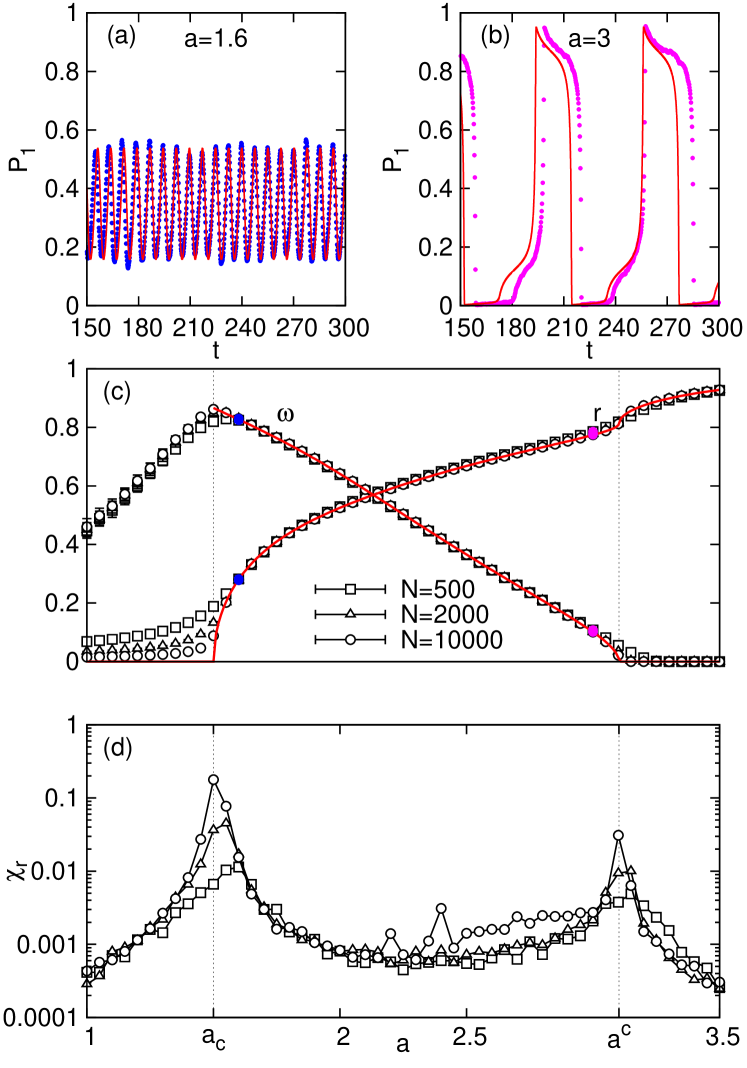
Figure 3: (Color online) Panels (a) and (b) show the evolution of $P_{1}$ for $a=1.6$ and $a=3$, respectively. Points represent simulations for complete graph with $N=10000$ whereas lines show the mean-field solution. (c) Dependence of $r$ and $\omega$ on $a$, exhibiting the two phase transitions. (d) $\chi_{r}$ versus $a$ showing peaks at the transitions [system sizes as in (c)].

2 Model

In the WCM, the phase $\phi_{x}$ at site $x$ ($x=1,\ldots,N$) can take one of three values: $\phi_{x}=j_{x}2\pi/3$, where $j_{x}\in\{0,1,2\}$ (for simplicity, from here on we employ $x$ to denote sites and $j$ to denote states — always modulo 3). The only allowed transitions are those from $j$ to $j+1$ (see Fig. 1), with transition rates

$$g_{j,j+1}=g\exp\left[\frac{a\left(N_{j+1}-N_{j}\right)}{z}\right],$$ (1)

where $g$ is a constant (which can be set to unity without loss of generality), $a$ is the coupling parameter, $N_{j}$ is the number of nearest neighbors in state $j$, and $z$ is the number of nearest neighbors. The rates are invariant under cyclic permutation of the indices, i.e., belong to the symmetry group $C_{3}$ of discrete rotations, and strongly violate the detailed balance condition.

The mean-field approximation is obtained by replacing $N_{j}/z$ in the argument of the exponential of Eq. 1 with the corresponding probability, $P_{j}$, leading to the following set of equations:

$$\dot{P}_{j}=g_{j-1,j}P_{j-1}-g_{j,j+1}P_{j}\;,$$ (2)

where now $g_{j,j+1}=g\exp\left[a\left(P_{j+1}-P_{j}\right)\right]$. These also represent the equations for a complete graph in the limit $N\to\infty$: since $z=N-1$, we can replace $N_{j}/N$ with $P_{j}$ in the infinite-size limit. Normalization reduces these equations to a two-dimensional flow in the $(P_{1},P_{2})$ plane (Fig. 2).

Starting from the complex order parameter,

$$v\equiv\frac{1}{N}\sum^{N}_{x=1}e^{i\phi_{x}}$$ (3)

one can define quantities that characterize the collective behavior of the system. A configuration with $v\neq 0$ has unequal numbers of sites in the three states, which led Kuramoto to propose

$$r\equiv\left<\left<|v|\right>_{t}\right>_{s}$$ (4)

as the order parameter for synchronization [1, 3, 12], where $\left<\right>_{t}$ denotes a time average over a single realization (in the stationary state), and $\left<\right>_{s}$ an average over independent realizations. Note that $r>0$ is consistent with, but does not necessarily imply, globally synchronized oscillations. The latter is characterized by a periodically varying phase of $v$ [16, 17, 18, 19].

In the mean-field equations (2), the transition to the synchronized regime is associated with a supercritical Hopf bifurcation at $a=a_{c}=1.5$. The trivial fixed point $\vec{P}_{1/3}^{*}\equiv(P_{1}=1/3,P_{2}=1/3)$ loses stability at $a=a_{c}$, and a limit cycle encircling this point appears (Fig. 2a-b) [12]. For $a\gtrsim a_{c}$, sustained oscillations in $P_{j}$ characterize synchronization among the oscillators (Fig. 3a). Correspondingly, $r$ grows continuously $\sim(a-a_{c})^{\beta}$ at the transition (Fig. 3c), with a mean-field exponent $\beta=1/2$ [12]. The scaled variance $\chi_{r}\equiv L^{d}\left[\left<\left<|v|\right>^{2}_{t}\right>_{s}-r^{2}\right]$ diverges with the system size at criticality, as shown for simulations of complete graphs using $L^{d}\equiv N$ in Fig. 3d.

Note that the phase transition to stable collective oscillations is associated with the breaking of the continuous time-translation symmetry: the time series $P_{0}(t)$, $P_{1}(t)$ and $P_{2}(t)$ become periodic for $a\gtrsim a_{c}$. But since they are statistically identical, except for a phase, $C_{3}$ symmetry still holds. Increasing $a$ above $a_{c}$ enhances synchronization among the oscillators, leading to increasing oscillation amplitudes, as shown in Figs. 2d and 3b.

3 The Second Phase Transition

3.1 Mean-field theory and the complete graph

Wood et al. found that the increasing amplitude of oscillation is accompanied by a decreasing angular frequency $\omega=2\pi/\langle\tau\rangle$, where $\langle\tau\rangle$ is the mean time between peaks in $P_{k}$ (Figs. 3a-c). This can be understood qualitatively from the exponential dependence of the rates of Eq. 1 on the neighbor fractions: when a state is highly populated, the rate at which oscillators leave this state becomes very small. In addition, the rate at which a highly populated state attracts oscillators from its predecessor is also very high.

We study the effect of a further increase in the coupling $a$, beyond the range of values investigated in Ref. [12], using mean-field theory and analysis on a complete graph of $N$ sites. Note that the state of the latter is completely specified by two integer random variables, $N_{1}$ and $N_{2}$. We study the complete graph (for $N$ up to 1000) via exact (numerical) stationary solution of the master equation [20] and (for $N$ ranging from 10 to 10⁴) via event-driven Monte Carlo simulations. The results of the two approaches are fully consistent.

In mean-field theory, when $a$ reaches an upper critical value $a^{c}\simeq 3.102\,439\,915\,64$, three symmetric saddle-node bifurcations occur simultaneously, and the period of the collective oscillations diverges. Above $a^{c}$, there are three symmetric attractors in the system, and 3-fold rotational ($C_{3}$) symmetry is spontaneously broken: Figure 2f illustrates how the final fate of three different trajectories starting from the same initial conditions is determined by fluctuations. Moreover, the transition can be considered reentrant, in the sense that time-translation symmetry, which had been broken at $a_{c}$, is restored at $a^{c}$ (although, unlike other cases seen in the literature [21, 22], the phase above $a^{c}$ is not exactly the same as that below $a_{c}$, because of $C_{3}$ symmetry breaking).

Analogously to what occurs in a condensation or ferromagnetic phase transition [23], the freezing of the relative occupancy of each state does not imply that individual oscillators freeze as well. The frequencies of individual oscillators do decrease with increasing $a$, but only vanish in the limit $a\to\infty$, when one of the states is fully occupied.

It is convenient to define an order parameter that is identically zero (in the infinite-size limit) for $a>a^{c}$. Since the angular frequency $\omega$ does not fulfill the usual requirements for an order parameter [24], we propose

$$|\psi|\equiv\frac{1}{N}\left|\sum_{x=1}^{N}\left(\delta_{0,j_{x}}+e^{2\pi i/3}\delta_{1,j_{x}}+e^{-2\pi i/3}\delta_{2,j_{x}}\right)\gamma_{x}\right|\;,$$ (5)

where $\delta$ is the Kronecker delta and $\gamma_{x}\equiv g_{j_{x},j_{x}+1}$ is the transition rate at site $x$ (see Eq. 1). Thus $|\psi|$ reflects not only the configuration, but the rate at which the latter evolves.

On the complete graph, $\gamma_{x}$ is the same for all sites $x$ in the same state $j$. Denoting this rate by $\gamma_{j}$, the order parameter can be rewritten for mean-field (MF) analysis as

$$|\psi|^{2}\stackrel{{\scriptstyle MF}}{{=}}\left[\sum_{j=0}^{2}P_{j}^{2}\gamma_{j}^{2}\right]-P_{0}\gamma_{0}P_{1}\gamma_{1}-P_{1}\gamma_{1}P_{2}\gamma_{2}-P_{2}\gamma_{2}P_{0}\gamma_{0}\;.$$ (6)

Note that both the disordered phase ($a<a_{c}$) as well as the frozen phase ($a>a^{c}$) have stable fixed points, so $P^{*}_{j}\gamma_{j}=P^{*}_{j+1}\gamma_{j+1}$ from Eq. 2. This in turn renders $|\psi|=0$ in Eq. 6 for both cases [a similar line of reasoning can be applied directly to Eq. (5)].

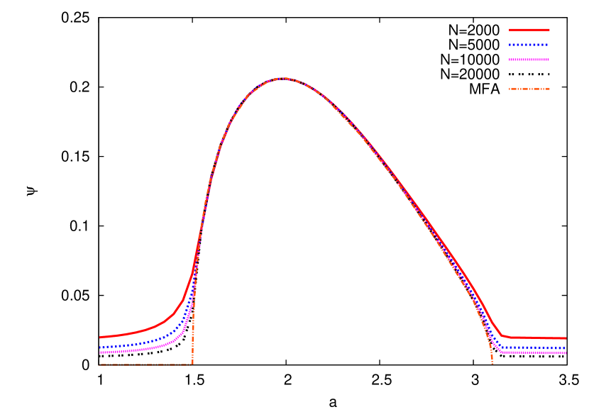
Figure 4: Order parameter $\langle|\psi|\rangle$ as a function of coupling $a$ in mean-field theory and on the complete graph, for sizes as indicated.

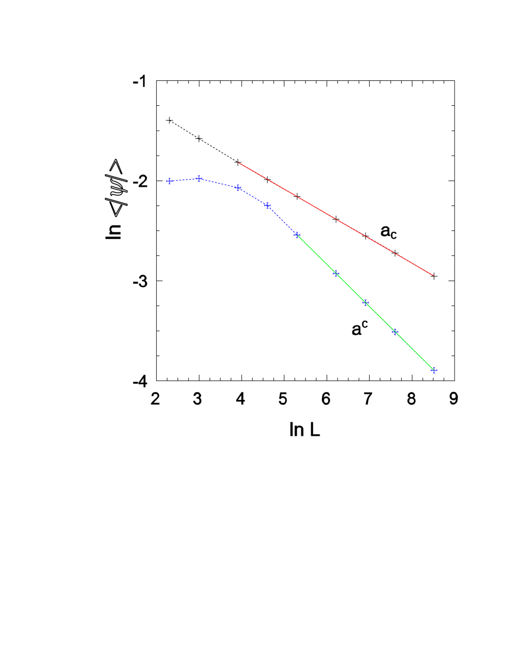
Figure 5: $\langle|\psi|\rangle$ at the critical points versus system size $N$ on the complete graph. The order parameter decays as a power law of the system size at both phase transitions.

Figure 4 shows the variation of $\langle|\psi|\rangle$ ($\equiv\langle\langle|\psi|\rangle_{t}\rangle_{s}$) with $a$ in mean-field theory, and on the complete graph, confirming that $|\psi|$ functions as an order parameter to detect both phase transitions. The MF critical behavior is $\langle|\psi|\rangle\sim(a-a_{c})^{1/2}$ for $a\swarrow a_{c}$ and $\langle|\psi|\rangle\sim(a^{c}-a)^{1/2}$ for $a\nearrow a^{c}$. In the pair approximation for a lattice with coordination number $z=6$ we find $a_{c}=1.97579$ and $a^{c}=4.71727$; for $z=8$ the corresponding values are $a_{c}=1.80198$ and $a^{c}=4.10028$. In the pair approximation, no transition is observed for $z\leq 4$.

On the complete graph, the order parameter decays with system size as $\langle|\psi|\rangle\sim N^{-1/4}$ at $a=a_{c}$ and as $N^{-0.4203(3)}$ at $a=a^{c}$, as shown in Fig. 5. The first result is typical of mean-field-like scaling with system size at a continuous phase transition, and can be understood as follows. Our numerical results show that with increasing $N$, as expected, the stationary probability distribution in the $P_{1}-P_{2}$ plane becomes (for $a=a_{c}$) increasingly concentrated around the symmetric point $(1/3,1/3)$. The maximum of the distribution, $p_{max}$, scales as $N^{-3/2}$ and the number of points at which the probability is relatively large (i.e., $p(N_{1},N_{2})\geq p_{max}/2$) grows $\sim N^{3/2}$. In terms of the densities $P_{i}=N_{i}/N$, the probability distribution is concentrated on a region of radius $\rho\sim N^{-1/4}$. Note that $|\psi|^{2}$ is a quadratic form of the variables $\xi_{i}\equiv P_{i}-1/3$ and that $\psi=0$ for $\xi_{1}=\xi_{2}=0$. Thus for the purposes of scaling analysis we may write the stationary average of $|\psi|$ as

$$\langle|\psi|\rangle\sim\frac{\int_{0}^{N^{-1/4}}\xi^{2}d\xi}{\int_{0}^{N^{-1/4}}\xi d\xi}\sim N^{-1/4}$$ (7)

with $\xi=\sqrt{\xi_{1}^{2}+\xi_{2}^{2}}$. At the first transition ($a=a_{c}$) the same argument applies to the order parameter $r$, and we indeed find numerically $r\sim N^{-0.26}$.

At the second transition, the probability distribution is peaked near the three stable fixed points of the mean-field analysis, and so has a very different form than that found at $a_{c}$. It is therefore not surprising that $\langle|\psi|\rangle$ decays with a different exponent. The value of 0.4203(3) (which does not correspond to any simple ratio of integers) nevertheless remains something of a puzzle. We suspect that understanding this result will require an asymptotic (large-$N$) analysis of the Fokker-Planck equation for the probability density in the $P_{1}-P_{2}$ plane, a task we defer to future work.

3.2 Hypercubic lattices

Motivated by the appearance of a novel phase transition in mean-field theory and on the complete graph, we search for such a transition on finite-dimensional structures, i.e., the simple cubic lattice and its four-dimensional (hypercubic) analog, in systems of $N=L^{d}$ sites. On these lattices, we do observe a marked tendency for $\omega$ to fall rapidly with $a$ for values well above the first transition at $a_{c}$ ($a_{c}\simeq 2.345$, $\simeq 1.900$ and $\simeq 1.750$ for $d=3$, 4 and 5, respectively [12]). We also observe a broad maximum in $\chi_{r}$ at some point in this range. To infer the existence of a phase transition, rather than a rapid but smooth variation of $\omega$ and other properties with $a$, we require evidence of emergent singularities as the linear system size $L$ is increased.

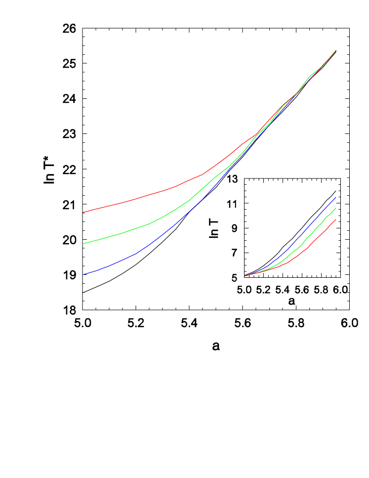
Figure 6: (Color online) Four dimensional hypercubic lattice: Inset mean period $T$ versus a for (upper to lower) $L=28$, 32, 40, and 50. Main graph: scale period $T^{*}\equiv L^{d}T$; system size increasing upwards.

The global dynamics may be characterized in terms of a process that begins with all sites in state $j$, and ends when the fraction of sites remaining this state falls to $\leq 1/3$. Let the “escape time” $T$ denote the mean duration this process, averaged over realizations of the stochastic dynamics. If there is an infinite-period phase transition at some critical value $a^{c}$, then $T$ should grow $\sim L^{z}$ at this point, where $z$ denotes the dynamic critical exponent. Although simulations reveal an exponential growth of $T$ with $a$ at fixed $L$, they show that for large, fixed $a$, the escape time decreases with increasing system size! The mean period (see Fig. 6) exhibits two regimes for $a>a_{c}$: for smaller $a$, relatively slow, exponential growth with $T\sim e^{a}$ essentially independent of system size, and, for larger $a$, rapid exponential growth with $T\sim L^{-d}e^{\kappa a}$, with $\kappa\gg 1$. We identify the latter regime as that of single-droplet nucleation [25]. In the former regime, the density of “advanced” sites (i.e., in state $j+1$ in a configuration with the majority in state $j$) is large enough that essentially no barrier to the cyclic dynamics exists. The (smooth) crossover between these regimes occurs at a larger $a$ value for larger system sizes.

The results for the mean transition rate $T$ on the four-dimensional hypercubic lattice, $T\sim L^{-d}\exp[\kappa a]$, clearly suggest a nucleation mechanism. The exponential factor represents a barrier to nucleation, that is, the mean time to formation of a critical cluster. (By a “critical” cluster we mean one that is equally likely to grow as to diminish in size; larger clusters tend to grow while smaller ones tend to shrink.) Consider a region in which all spins are in the same state. The rate at which a given spin flips to the next state (e.g., 1 $\to$ 2) is $e^{-a}$ leading to the exponential growth in $T$. The prefactor $1/L^{d}$ corresponds to essentially independent contributions due to each site in the system. (Given the extremely low density of clusters in this regime, we can treat the nucleation and initial growth of a cluster as occurring in isolation, without interference from other clusters.)

Figure 7: Square lattice, $L=10$: evolution of $N_{1}$ (main graph) and $N_{2}$ (inset) in a typical realization with $a=8$.

The constant $\kappa$ in the exponential reflects the probability of formation of a critical cluster, which in turn depends on the critical cluster size, $\ell^{*}$. Intuitively, the nucleation barrier exists because an isolated advanced site has a higher rate to advance once again, and then rapidly return to the majority state, than it does of inducing a neighbor to advance. Given the difficulty of visualizing four-dimensional space, we begin by studying nucleation on the square lattice. Of course, the model does not exhibit an ordered phase in two dimensions, but this issue can be bypassed by using small systems (a lattice of 10$\times$10 sites, in the present case). Then the system remains near one of the three attractors (almost all sites in the same state) except for the rapid transitional periods following a nucleation event. (In larger systems global synchronization is quickly lost and the system breaks into a number of domains.) On such a small lattice, one may easily identify transitional regimes between, for example, states with majority-1 and majority-2. We define the transition (in the macroscopic sense) as the moment when 20% of sites are in state 1, with nearly all the rest (70% or more) in state 2. To estimate $T$ we determine the time required for a large number (4000, in practice) of transitions to occur, in event-driven Monte Carlo simulations. A typical evolution is shown in Fig. 7. We find that the mean transition time grows exponentially with $a$; for $a\geq 7$ we find $\kappa=1.68(1)$. This suggests that the critical cluster size is approximately 3 - 4.

Several other pieces of evidence support this estimate. First, in the pre-transition regime, the number $N_{2}$ of sites in state 2 is seen to fluctuate between zero and three or so. In the example shown in Fig. 7, the second time $N_{2}$ grows to four, a transition occurs. Typical formats of a growing cluster are shown in Fig. 8; the cluster is seen to be compact, as expected for a growth probability that is highest for the sites outside the cluster having the largest number of neighbors within it.

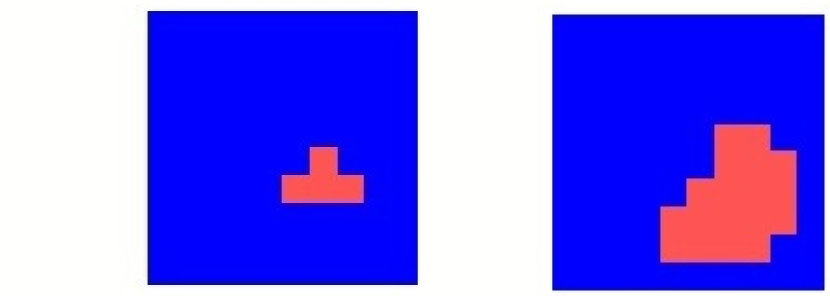
Figure 8: (Color online) Typical evolution of a cluster of 2s (red) in a background of 1s (blue). Square lattice, $L=10$, $a=6$, times $t=39$ (left) and 58 (right).

A semiquantitative analysis of the cluster size distribution in the pretransition regime can be developed as follows. Consider first the density $\rho_{2}$ of isolated sites in state 2, in a background of 1s. The rate for a given 1 to change to 2 is $e^{-a}$, while an isolated 2 (with all neighbors in state 1) flips to state 3 at unit rate. There are also transitions of the form 21 $\to$ 22. The total rate for an isolated 2 to become a dimer is $4e^{-a/2}$. Thus we have a rate equation of the form

$$\dot{\rho}_{2}=e^{-a}\rho_{1}-\rho_{2}-4e^{-a/2}\rho_{1}\rho_{2}\simeq e^{-a}-\rho_{2}$$ (8)

leading to $\rho_{2}\simeq e^{-a}$ in the quasi-stationary (QS) regime. By the QS regime we mean the long-lived metastable state in which the great majority of sites are in state 1. Similarly, let $\rho_{22}$ denote the probability that a given site is the leftmost (or lowermost) site of an isolated dimer (the restriction is to avoid double counting). Then we have

$$\dot{\rho}_{22}\simeq 4e^{-a/2}\rho_{2}-2e^{-a/4}\rho_{22}-{\cal O}(e^{-a/2}\rho_{22})$$ (9)

so that $\rho_{22}\simeq 2e^{-5a/4}$ in the QS state. Consider next the density $\rho_{\sf L}$ of L-shaped trimers. The gain term in the equation for $\rho_{\sf L}$ is $4e^{-a/2}\rho_{22}$ while the dominant loss term (due to formation of a four-site, square cluster) is simply $-\rho_{\sf L}$ (the transition rate is unity). Thus $\rho_{\sf L}\simeq 8e^{-7a/4}$. The exponential factor, $e^{-7a/4}$, is quite close to the factor $e^{-1.68(1)a}$ found in simulations, suggesting that this is essentially the critical cluster. (Note that this is the smallest cluster with a larger probability of growing than of shrinking.) Applied to the simple cubic lattice, this line of reasoning suggests that the critical cluster consists of seven sites (in the form of a cube with one corner removed) and yields $\kappa_{3}=11/3$. [A crude estimate for the value in four dimensions can be obtained by supposing that $\kappa_{4}\approx(\kappa_{3}/\kappa_{2})\times\kappa_{3}$; this yields $\kappa_{4}\approx 7.7$, reasonably close to the simulation value, $\kappa_{4}=8.43(7)$.]

The nucleation scenario outlined above essentially rules out the second transition on any finite-dimensional lattice with short-range interactions. There is always a cluster size such that growth is more likely than shrinkage, and once such a cluster forms, a transition of the global state is likely. From the perspective of equilibrium phase transitions, this is not surprising: the ordered state of any (finite) Ising or Potts model is always subject to a reversal of magnetization at a finite rate. (This rate, however, decays with system size in equilibrium, as a finite cluster is always more likely to shrink than to grow, in the absence of an external field.) In the present cyclic dynamics, by contrast, there is no impediment to growth (no “surface tension”, as it were), once a cluster has attained the critical size.

4 Conclusions

We have identified a second phase transition in the cyclic model proposed by Wood et al. [12, 13, 14, 15] This continuous transition is of a fundamentally different nature than the first, as it corresponds to an infinite-period transition at which macroscopic properties freeze and a discrete rotational ($C_{3}$) symmetry is spontaneously broken, in the absence of an absorbing state. We find that an appropriate order parameter for the second transition involves the local transition rates. While the phase transition is observed on the complete graph, we argue that it does not exist on finite-dimensional structures with short-range interactions. The question naturally arises whether such an infinite-period transition exists in systems with long-range interactions. This indeed appears likely, for interactions that decay sufficiently slowly with distance. In the case of graphs with interactions between many pairs of sites, independent of distance, we expect to observe an infinite-period transition if (in the infinite-size limit) a given site interacts with a finite fraction of the others. We plan to investigate these questions, as well as the behavior on scale-free networks, in future work.

5 Acknowledgments

VRVA and MC acknowledge financial support from CNPq, FACEPE, CAPES, FAPERJ and special programs PRONEX, PRONEM and INCEMAQ. RD acknowledges financial support from CNPq.

References

- [1] Y. Kuramoto, editor. Chemical Oscillations, Waves and Turbulence. Dover, Berlin, 1984.
- [2] SH Strogatz and I Stewart. Coupled oscillators and biological synchronization. Sci. Am., 269(6):102–109, 1993.
- [3] S. H. Strogatz. From Kuramoto to Crawford: Exploring the onset of synchronization in populations of coupled oscillators. Physica D, 143:1–20, 2000.
- [4] S. H. Strogatz. Sync: How Order Emerges From Chaos In the Universe, Nature, and Daily Life. Hyperion, New York, 2004.
- [5] A. Pikovsky, M. Rosenblum, and J. Kurths. Synchronization: A Universal Concept in Nonlinear Sciences. Cambridge University Press, Cambridge, UK, 2001.
- [6] P. Reimann, C. Van den Broeck, and R. Kawai. Nonequilibrium noise in coupled phase oscillators. Phys. Rev. E, 60(6):6402–6406, 1999.
- [7] K. Tainaka. Lattice model for the Lotka-Volterra system. J. Phys. Soc. Japan, 57(8):2588–2590, 1988.
- [8] K. Tainaka. Stationary pattern of vortices or strings in biological systems: Lattice version of the Lotka-Volterra model. Phys. Rev. Lett., 63(24):2688–2691, 1989.
- [9] K. Tainaka and Itoh Y. Topological phase transition in biological ecosystems. Europhys. Lett., 15(4):399–404, 1991.
- [10] Y. Itoh and K. Tainaka. Stochastic limit cycle with power-law spectrum. Phys. Lett. A, 189:37–42, 1994.
- [11] K. Tainaka. Vortices and strings in a model ecosystem. Phys. Rev. E, 50(5):3401, 1994.
- [12] K. Wood, C. Van den Broeck, R. Kawai, and K. Lindenberg. Universality of synchrony: Critical behavior in a discrete model of stochastic phase-coupled oscillators. Phys. Rev. Lett., 96:145701, 2006.
- [13] K. Wood, C. Van den Broeck, R. Kawai, and K. Lindenberg. Critical behavior and synchronization of discrete stochastic phase-coupled oscillators. Phys. Rev. E, 74(3):031113, 2006.
- [14] K. Wood, C. Van den Broeck, R. Kawai, and K. Lindenberg. Effects of disorder on synchronization of discrete phase-coupled oscillators. Phys. Rev. E, 75(4):041107, 2007.
- [15] K. Wood, C. Van den Broeck, R. Kawai, and K. Lindenberg. Continuous and discontinuous phase transitions and partial synchronization in stochastic three-state oscillators. Phys. Rev. E, 76(4):041132, 2007.
- [16] Y. Kuramoto, T. Aoyagi, I. Nishikawa, T. Chawanya, and K. Okuda. Neural Network Model Carrying Phase Information with Application to Collective Dynamics. Prog. Theor. Phys., 87:1119–1126, 1992.
- [17] H. Ohta and S. Sasa. Critical phenomena in globally coupled excitable elements. Phys. Rev. E, 78(6):065101, 2008.
- [18] S. Shinomoto and Y. Kuramoto. Phase transitions in active rotator systems. Progr. Theoret. Phys., 75(5):1105–1110, 1986.
- [19] F. Rozenblit and M. Copelli. Collective oscillations of excitable elements: order parameters, bistability and the role of stochasticity. J. Stat. Mech., 2011:P01012, 2011.
- [20] R. Dickman. Numerical analysis of the master equation. Phys. Rev. E, 65(4):047701, 2002.
- [21] C. Van den Broeck, J. M. R. Parrondo, R. Toral, and R. Kawai. Nonequilibrium phase transitions induced by multiplicative noise. Phys. Rev. E, 55(4):4084–4094, 1997.
- [22] R. Kawai, X. Sailer, L. Schimansky-Geier, and C. Van den Broeck. Macroscopic limit cycle via pure noise-induced phase transitions. Phys. Rev. E, 69(5):051104, 2004.
- [23] K. Huang. Statistical Mechanics. John Wiley & Sons, 1987.
- [24] M. Plischke and B. Bergersen. Equilibrium Statistical Physics. World Scientific Publishing Company, 2nd edition, 1994.
- [25] P. A. Rikvold, H. Tomita, S. Miyashita, and S. W. Sides. Metastable lifetimes in a kinetic ising model: Dependence on field and system size. Phys. Rev. E, 49(6):5080–5090, 1994.