Constraints on exotic lepton doublets with minimal coupling to the standard model

Abstract

We investigate the consequences of introducing a set of exotic doublet leptons which couple to the standard model leptons in a minimal way. Through these additional gauge invariant and renormalizable coupling terms, new sources of tree-level flavor changing currents are induced via mixing. In this work, we derive constraints on the parameters that govern the couplings to the exotic doublets by invoking the current low-energy experimental data on processes such as leptonic $Z$ decays, $\ell\rightarrow 3\ell^{\prime}$, $\ell\rightarrow\ell^{\prime}\gamma$, and $\mu$-$e$ conversion in atomic nuclei. Moreover, we have analyzed the role these doublets play on the lepton anomalous magnetic moments, and found that their contribution is negligible.

I Introduction

It is well-known that the phenomenon of neutrino oscillations neutrinos_exp have motivated an extensive study on models with nonzero neutrino masses and lepton flavor violation (LFV). Central to all these investigations is the introduction of new interactions (and most likely new particles too) to the minimal standard model (SM). While there can be many different ways of inventing and restricting the new physics, recently in Chua:2010me , a fairly economical approach based on only SM gauge invariance, renormalizability and the concept of “minimal coupling” was considered for the lepton sector.

In that work, a generic minimal coupling between SM particles and some exotic field was defined to have the form

$$Y_{\text{exotic}}\;\text{(SM particle)}\cdot\text{(SM particle)}\cdot\text{(exotic particle)}\;,$$ (1)

where $Y_{\text{exotic}}$ denotes the coupling strength and the “exotic particle” can either be a scalar boson, a fermion or a vector boson. All particles in (1) are assumed to be uncolored in the $SU(3)_{c}$ sense because we only wish to extend the lepton sector. These minimal interactions are of interest because they are relatively simple and their collider signatures may be detected at the LHC in the near future under favorable conditions DelNobile:2009st .

Schematically, there are five distinct types of interaction with the SM fields allowed by (1) and the requirement of renormalizability,

$$\text{(i)}\;\;L_{L}\times L_{L}\times[\text{new}]\;,\;\;\text{(ii)}\;\;L_{L}\times\ell_{R}\times[\text{new}]\;,\;\;\text{(iii)}\;\;\ell_{R}\times\ell_{R}\times[\text{new}]\;,$$

$$\text{(iv)}\;\;L_{L}\times\phi\times[\text{new}]\;,\;\;\text{(v)}\;\;\ell_{R}\times\phi\times[\text{new}]\;.$$ (2)

where $L_{L}=(\nu_{L},\ell_{L})^{T}$ is the left-handed (LH) lepton doublet, $\ell_{R}$ is the right-handed (RH) lepton singlet, and $\phi=(\phi^{+},\phi^{0})^{T}$ denotes the SM Higgs doublet. The imposition of Lorentz and SM gauge symmetries will then result in only 13 types of exotic multiplets that are minimally coupled to the SM particles (see Table 1).

As pointed out in Chua:2010me , it seems that all but two types of the new particles induced by this setup has already been heavily analyzed because of various motivations. The two that are rarely discussed are the exotic lepton triplets $E_{R,L}=(E^{0}_{L,R},E^{-}_{L,R},E^{--}_{L,R})^{T}$ and the doublets $\widetilde{L}_{L,R}=(\widetilde{L}^{-}_{L,R},\widetilde{L}^{--}_{L,R})^{T}$ with SM quantum numbers $(1,3,-1)$ and $(1,2,-3/2)$ respectively. Whereas the study of the triplets $E_{R,L}$ formed the backbone of Chua:2010me , we shall concentrate on the last remaining possibility—doublets $\widetilde{L}_{L,R}$ in this work.

The various implications of introducing $\widetilde{L}_{L,R}$ to the SM are studied in the subsequent sections. Processes such as $Z$ decays (Sec. III), LFV decays: $\ell\rightarrow 3\ell^{\prime}$ (Sec. IV), $\ell\rightarrow\ell^{\prime}\gamma$ (Sec. V), and $\mu$-$e$ conversion in atomic nuclei (Sec. VI) are considered with the aim to derive constraints on the relevant new physics parameters using low-energy experimental data (Sec. VII). The contributions from $\widetilde{L}_{L,R}$ to the lepton anomalous magnetic moments will be investigated in Sec. VIII. Finally, in Sec. IX, we will make some brief comments regarding their collider phenomenologies.

[new]	spin	$SU(2)_{L}$	$U(1)_{Y}$	type	SM fields involved	studied in
$\Phi_{i}$	0	2	$1/2$	(ii)	$\overline{L}_{L}\;\;\ell_{R}$	multi-Higgs doublet models multi_Higgs_models ; rad_seesaw_eg
$\chi_{0}$	0	1	$-1$	(i)	$\overline{L}_{L}\;\;L_{L}^{c}$	dilepton/Babu-Zee models rad_seesaw_eg ; dileptons1 ; dileptons2 ; babu_zee
$\Delta$	0	3	$-1$	(i)	$\overline{L}_{L}\;\;L_{L}^{c}$	dilepton/Type-II seesaw dileptons1 ; doubly_Higg ; type2seesaw ; Abada:2007ux
$\xi_{0}$	0	1	2	(iii)	$\overline{\ell}_{R}\;\;\ell_{R}^{c}$	dilepton/Babu-Zee models dileptons1 ; dileptons2 ; babu_zee ; babu_zee2
$\nu_{R}$	1/2	1	$0$	(iv)	$\overline{L}_{L}\;\;\phi^{c}$	Type-I seesaw Abada:2007ux ; type1seesaw ; Biggio:2008in ; type1_3 ; type1set2
$\Sigma_{R}$	1/2	3	$0$	(iv)	$\overline{L}_{L}\;\;\phi^{c}$	Type-III seesaw Abada:2007ux ; type1_3 ; type3seesaw ; Abada:2008ea
$L_{L}^{\prime\prime}$	1/2	2	$-1/2$	(v)	$\overline{\ell}_{R}\;\;\phi^{\dagger}$	4th generation leptons 4thgen
$\ell_{R}^{\prime\prime}$	1/2	1	$-1$	(iv)	$\overline{L}_{L}\;\;\phi$	4th generation leptons 4thgen
$E_{R,L}$	1/2	3	$-1$	(iv)	$\overline{L}_{L}\,\phi\;$ ($E_{R}$ only)	see Chua:2010me ; Delgado:2011iz
$\widetilde{L}_{L,R}$	1/2	2	$-3/2$	(v)	$\overline{\ell}_{R}\,(\phi^{c})^{\dagger}$ ($\widetilde{L}_{L}$ only)	rarely discussed
$Z_{\mu}^{\prime}$	1	1	$0$	(i) & (iii)	$\overline{L}_{L}\;\;L_{L}\;$ and $\;\overline{\ell}_{R}\;\;\ell_{R}$
$X_{\mu}$	1	2	$-3/2$	(ii)	$\overline{L}_{L}\;\;\ell_{R}^{c}$	GUT/dilepton boson models dileptons1 ; dilepton_boson
$W_{\mu}^{\prime}$	1	3	$0$	(i)	$\overline{L}_{L}\;\;L_{L}$

Table 1: Summary of the 13 types of exotic multiplets induced by the 5 general types of minimal couplings: (i) $L_{L}\times L_{L}\times[\text{new}]$, (ii) $L_{L}\times\ell_{R}\times[\text{new}]$, (iii) $\ell_{R}\times\ell_{R}\times[\text{new}]$, (iv) $L_{L}\times\phi\times[\text{new}]$, and (v) $\ell_{R}\times\phi\times[\text{new}]$. Hypercharges are defined with $Q=I_{3}+Y$.

II Model with exotic lepton doublets, $\widetilde{L}_{L,R}$

We begin by writing down the framework and explaining our notations for our minimally extended SM with exotic lepton doublets. In this model, we have two new sets (LH and RH) of lepton doublets $\widetilde{L}_{L,R}$, all having hypercharge $-3/2$ (where $Q=I_{3}+Y$). In matrix form, they are given by

$$\widetilde{L}_{L}=\begin{pmatrix}\widetilde{L}^{-}_{L}\\ \widetilde{L}^{--}_{L}\end{pmatrix}\;,\qquad\widetilde{L}_{R}=\begin{pmatrix}\widetilde{L}^{-}_{R}\\ \widetilde{L}^{--}_{R}\end{pmatrix}\;\sim(1,2,-3/2)\;,$$ (3)

where $\widetilde{L}_{L}$ and $\widetilde{L}_{R}$ are independent fields. The interaction Lagrangian of interest is

$$\widetilde{\mathcal{L}}=\overline{\widetilde{L}_{L}}i\not{D}\widetilde{L}_{L}+\overline{\widetilde{L}_{R}}i\not{D}\widetilde{L}_{R}-\left[\overline{\widetilde{L}_{L}}\widetilde{M}\widetilde{L}_{R}+\overline{\widetilde{L}_{L}}\widetilde{Y}^{\dagger}\phi^{c}\ell_{R}+\overline{L}_{L}Y_{\ell}\phi\,\ell_{R}+\overline{L}_{L}Y_{\nu}\phi^{c}\,\nu_{R}+h.c.\right]\;,$$ (4)

where $\phi^{c}=(\phi^{0*},-\phi^{-})^{T}$, and the covariant derivative is defined as,

$$\not{D}=\not{\partial}-\frac{ig}{\sqrt{2}}\left[\not{W}^{+}\begin{pmatrix}0&1\\ 0&0\end{pmatrix}+\not{W}^{-}\begin{pmatrix}0&0\\ 1&0\end{pmatrix}\right]-\frac{ig}{\cos\theta_{w}}\not{Z}(I_{3}-\sin^{2}\theta_{w}Q)+ie\not{A}Q\;,\quad(e>0)\;,$$ (5)

with $Q$ and $I_{3}$ being the operators for electric charge and the 3rd component of isospin respectively. In (4), the Yukawa term involving $\widetilde{Y}^{\dagger}$ defines the minimal coupling between $\ell_{R}$ and $\widetilde{L}_{L}$ while $\widetilde{M}$ sets the energy scale of the new physics. Notice that one cannot have a similar type of minimal coupling between $\widetilde{L}_{R}$ and any other SM leptons because of SM gauge invariance. But its effects on the SM sector can enter indirectly via the mass term $\overline{\widetilde{L}_{L}}\widetilde{M}\widetilde{L}_{R}$. Writing out all the relevant interactions in (4), we have

$$\widetilde{\mathcal{L}}+\mathcal{L}^{\text{SM}}=\mathcal{L}^{W}+\mathcal{L}^{Z}+\mathcal{L}^{\text{mass}}+\mathcal{L}^{H}+\cdots\;,$$ (6)

where

$$\mathcal{L}^{W} =\frac{g}{\sqrt{2}}\left[\overline{\nu}_{L}\not{W}^{+}\ell_{L}+\overline{\widetilde{L}^{-}_{L}}\not{W}^{+}\widetilde{L}^{--}_{L}+\overline{\widetilde{L}^{-}_{R}}\not{W}^{+}\widetilde{L}^{--}_{R}\right]+h.c.\;,$$ (7)

$$\mathcal{L}^{Z} =\frac{g}{\cos\theta_{w}}\left[\frac{1}{2}\;\overline{\nu}_{L}\not{Z}\nu_{L}+\left(-\frac{1}{2}+\sin^{2}\theta_{w}\right)\overline{\ell}_{L}\not{Z}\ell_{L}+\sin^{2}\theta_{w}\;\overline{\ell}_{R}\not{Z}\ell_{R}+\left(\frac{1}{2}+\sin^{2}\theta_{w}\right)\overline{\widetilde{L}^{-}_{L}}\not{Z}\widetilde{L}^{-}_{L}\right.$$

$$\qquad\qquad\quad\left.+\left(\frac{1}{2}+\sin^{2}\theta_{w}\right)\overline{\widetilde{L}^{-}_{R}}\not{Z}\widetilde{L}^{-}_{R}+\left(-\frac{1}{2}+2\sin^{2}\theta_{w}\right)\overline{\widetilde{L}^{--}_{L}}\not{Z}\widetilde{L}^{--}_{L}+\left(-\frac{1}{2}+2\sin^{2}\theta_{w}\right)\overline{\widetilde{L}^{--}_{R}}\not{Z}\widetilde{L}^{--}_{R}\right]\;,$$ (8)

$$\mathcal{L}^{\text{mass}} =-\overline{\widetilde{L}^{-}_{L}}\widetilde{M}\widetilde{L}^{-}_{R}-\overline{\widetilde{L}^{--}_{L}}\widetilde{M}\widetilde{L}^{--}_{R}-\frac{v}{\sqrt{2}}\overline{\widetilde{L}^{-}_{L}}\,\widetilde{Y}^{\dagger}\,\ell_{R}-\overline{\ell}_{L}m_{\ell}\ell_{R}-\overline{\nu}_{L}m_{D}\nu_{R}+h.c.\;,$$ (9)

$$\mathcal{L}^{H} =-\frac{1}{\sqrt{2}}\overline{\widetilde{L}^{-}_{L}}\widetilde{Y}^{\dagger}\ell_{R}H-\frac{1}{v}\overline{\ell}_{L}m_{\ell}\ell_{R}H-\frac{1}{v}\overline{\nu}_{L}m_{D}\nu_{R}H+h.c.\;.$$ (10)

In getting (9) and (10), we have written $\phi=(\phi^{+},\phi^{0})^{T}\equiv(\phi^{+},(v+H+i\eta)/\sqrt{2})^{T}$, where $v$ is the Higgs vacuum expectation value (chosen to be real), $\eta$ and $\phi^{\pm}$ are the would-be Goldstone bosons. Also, we have defined $m_{\ell}\equiv vY_{\ell}/\sqrt{2}$ and $m_{D}\equiv vY_{\nu}/\sqrt{2}$.

The mixing between the SM charged leptons and components of the exotic doublet may be readily derived if we write the relevant terms in $\mathcal{L}^{\text{mass}}$ in matrix form:

$$\mathcal{L}^{\text{mass}} =-\frac{1}{2}\begin{pmatrix}\overline{\nu}_{L}&\overline{(\nu_{R})^{c}}\end{pmatrix}\begin{pmatrix}m_{D}&0\\ 0&m_{D}^{T}\end{pmatrix}\begin{pmatrix}\nu_{R}\\ (\nu_{L})^{c}\end{pmatrix}-\begin{pmatrix}\overline{\ell}_{L}&\overline{\widetilde{L}^{-}_{L}}\end{pmatrix}\begin{pmatrix}m_{\ell}&0\\ v\widetilde{Y}^{\dagger}/\sqrt{2}&\widetilde{M}\end{pmatrix}\begin{pmatrix}\ell_{R}\\ \widetilde{L}^{-}_{R}\end{pmatrix}$$

$$\qquad-\frac{1}{2}\begin{pmatrix}\overline{\widetilde{L}^{--}_{L}}&\overline{(\widetilde{L}^{--}_{R})^{c}}\end{pmatrix}\begin{pmatrix}\widetilde{M}&0\\ 0&\widetilde{M}^{T}\end{pmatrix}\begin{pmatrix}\widetilde{L}^{--}_{R}\\ (\widetilde{L}^{--}_{L})^{c}\end{pmatrix}+\cdots\;,$$ (11)

where we have used the fact that $\overline{\psi_{1}}\psi_{2}\equiv\overline{\psi_{2}^{c}}\psi_{1}^{c}$ for any fermion field $\psi_{1,2}$. One may define the following unitary transformations to bring all fields into their mass eigenbasis:

$$\begin{pmatrix}\nu_{L,R}\\ (\nu_{R,L})^{c}\end{pmatrix}=V_{L,R}\begin{pmatrix}\nu_{L,R}\\ (\nu_{R,L})^{c}\end{pmatrix}_{m}\;,\quad\begin{pmatrix}\ell_{L,R}\\ \widetilde{L}_{L,R}^{-}\end{pmatrix}=U_{L,R}\begin{pmatrix}\ell_{L,R}\\ \widetilde{L}_{L,R}^{-}\end{pmatrix}_{m}\;,\quad\begin{pmatrix}\widetilde{L}^{--}_{L,R}\\ (\widetilde{L}^{--}_{R,L})^{c}\end{pmatrix}=I_{n}\begin{pmatrix}\widetilde{L}^{--}_{L,R}\\ (\widetilde{L}^{--}_{R,L})^{c}\end{pmatrix}_{m}\;,$$ (12)

where the subscript $m$ indicates the mass basis. In (12), $V_{L,R},U_{L,R}$ and $I_{n}$ have dimensions $6\times 6,(3+n)\times(3+n)$ and $n\times n$ respectively, with $n$ being the number of generations of the exotic $\widetilde{L}_{L,R}$ fields added to the model.

Without loss of generality, one can choose to work in the basis where $m_{\ell}$ and $\widetilde{M}$ are real and diagonal. As a result, $I_{n}$ is in fact the identity matrix. Furthermore, to make the notations less cluttered, we absorb the neutrino right diagonalization matrix $U_{\nu R}$ into $m_{D}$. In other words, we set $m_{D}\equiv m_{D}^{\prime}U_{\nu R}$, where $U_{\nu L}^{\dagger}m_{D}^{\prime}U_{\nu R}=m_{D}^{\text{diag}}$ and $U_{\nu L}$ is the neutrino left diagonalization matrix. With these conventions, and to $\mathcal{O}\left(v^{2}\widetilde{M}^{-2}\right)$, the transformation matrices are given by

$$V_{L}=\begin{pmatrix}U_{\nu L}&0\\ 0&1\end{pmatrix}\;, \qquad V_{R}=\begin{pmatrix}1&0\\ 0&U_{\nu L}^{*}\end{pmatrix}\;,$$ (13)

$$U_{L}=\begin{pmatrix}1&v\,m_{\ell}\widetilde{Y}\widetilde{M}^{-2}/\sqrt{2}\\ -v\widetilde{M}^{-2}\widetilde{Y}^{\dagger}m_{\ell}/\sqrt{2}&1\end{pmatrix}\;, \qquad U_{R}=\begin{pmatrix}1-\lambda&v\widetilde{Y}\widetilde{M}^{-1}/\sqrt{2}\\ -v\widetilde{M}^{-1}\widetilde{Y}^{\dagger}/\sqrt{2}&1-\lambda^{\prime}\end{pmatrix}\;,$$ (14)

where

$$\lambda\equiv\frac{v^{2}}{2}\,\widetilde{Y}\,\widetilde{M}^{-2}\,\widetilde{Y}^{\dagger}\;,\quad\text{ and }\quad\lambda^{\prime}\equiv\frac{v^{2}}{2}\widetilde{M}^{-1}\,\widetilde{Y}^{\dagger}\,\widetilde{Y}\widetilde{M}^{-1}\,\;,$$ (15)

are $3\times 3$ and $n\times n$ matrices in flavor space respectively. Note that $U_{\nu L}$ may be identified as the usual neutrino mixing matrix, $U_{\text{PMNS}}$.

The relevant terms in the interaction Lagrangian with respect to the mass eigenbasis are therefore given by

$$\mathcal{L}^{W} =\frac{g}{\sqrt{2}}\left[\begin{pmatrix}\overline{\nu}&\overline{\nu^{c}}\end{pmatrix}_{m}\not{W}^{+}\left[P_{L}\,g_{1L}^{W}+P_{R}\,g_{1R}^{W}\right]\begin{pmatrix}\ell\\ \widetilde{L}^{-}\end{pmatrix}_{m}+\begin{pmatrix}\overline{\ell}&\overline{\widetilde{L}^{-}}\end{pmatrix}_{m}\not{W}^{+}\left[P_{L}\,g_{2L}^{W}+P_{R}\,g_{2R}^{W}\right]\begin{pmatrix}\widetilde{L}^{--}\\ (\widetilde{L}^{--})^{c}\end{pmatrix}_{m}\right]+h.c.,$$ (16)

$$\mathcal{L}^{Z} =\frac{g}{\cos\theta_{w}}\left[\begin{pmatrix}\overline{\nu}&\overline{\nu^{c}}\end{pmatrix}_{m}\not{Z}\,P_{L}\,g_{1L}^{Z}\begin{pmatrix}\nu\\ \nu^{c}\end{pmatrix}_{m}+\begin{pmatrix}\overline{\ell}&\overline{\widetilde{L}^{-}}\end{pmatrix}_{m}\not{Z}\left[P_{L}\,g_{2L}^{Z}+P_{R}\,g_{2R}^{Z}\right]\begin{pmatrix}\ell\\ \widetilde{L}^{-}\end{pmatrix}_{m}\right.$$

$$\qquad\qquad\qquad\left.+\begin{pmatrix}\overline{\widetilde{L}^{--}}&\overline{(\widetilde{L}^{--})^{c}}\end{pmatrix}_{m}\not{Z}\,P_{L}\,g_{3L}^{Z}\begin{pmatrix}\widetilde{L}^{--}\\ (\widetilde{L}^{--})^{c}\end{pmatrix}_{m}\right]\;,$$ (17)

$$\mathcal{L}^{H} =\begin{pmatrix}\overline{\nu}&\overline{\nu^{c}}\end{pmatrix}_{m}H\,P_{R}\,g_{1R}^{H}\,\begin{pmatrix}\nu\\ \nu^{c}\end{pmatrix}_{m}+\begin{pmatrix}\overline{\ell}&\overline{\widetilde{L}^{-}}\end{pmatrix}_{m}H\left[P_{L}\,g_{2L}^{H}+P_{R}\,g_{2R}^{H}\right]\begin{pmatrix}\ell\\ \widetilde{L}^{-}\end{pmatrix}_{m}\;,$$ (18)

with the new generalized coupling matrices given by (to leading order)

$$g_{1L}^{W} =\begin{pmatrix}U_{\nu L}^{\dagger}&v\,U_{\nu L}^{\dagger}m_{\ell}\widetilde{Y}\widetilde{M}^{-2}/\sqrt{2}\\ 0&0\end{pmatrix}\;,\quad g_{2L}^{W}=\begin{pmatrix}-v\,m_{\ell}\widetilde{Y}\widetilde{M}^{-2}/\sqrt{2}&0\\ 1&0\end{pmatrix}\;,\quad g_{1R}^{W}=0\;,\quad g_{2R}^{W}=\begin{pmatrix}-v\,\widetilde{Y}\widetilde{M}^{-1}/\sqrt{2}&0\\ 1-\lambda^{\prime}&0\end{pmatrix}\;,$$ (19)

$$g_{1L}^{Z} =\begin{pmatrix}1/2&0\\ 0&0\end{pmatrix}\;,\;g_{2L}^{Z}=\begin{pmatrix}-1/2+\sin^{2}\theta_{w}&-v\,m_{\ell}\widetilde{Y}\widetilde{M}^{-2}/\sqrt{2}\\ -v\,\widetilde{M}^{-2}\widetilde{Y}^{\dagger}m_{\ell}/\sqrt{2}&1/2+\sin^{2}\theta_{w}\end{pmatrix}\,,\;g_{3L}^{Z}=\begin{pmatrix}-1/2+2\sin^{2}\theta_{w}&0\\ 0&1/2-2\sin^{2}\theta_{w}\end{pmatrix}\;,$$

$$g_{2R}^{Z} =\begin{pmatrix}\sin^{2}\theta_{w}+(1/2-\sin^{2}\theta_{w})\lambda&-v\,\widetilde{Y}\widetilde{M}^{-1}/2\sqrt{2}\\ -v\,\widetilde{M}^{-1}\widetilde{Y}^{\dagger}/2\sqrt{2}&1/2+\sin^{2}\theta_{w}-(1+\sin^{2}\theta_{w})\lambda^{\prime}\end{pmatrix}\;,$$ (20)

$$g_{1R}^{H} =\begin{pmatrix}-U_{\nu L}^{\dagger}m_{D}/v&0\\ 0&0\end{pmatrix}\;,\;g_{2R}^{H}=\begin{pmatrix}m_{\ell}(2\lambda-1)/v&-m_{\ell}\,\widetilde{Y}\widetilde{M}^{-1}/\sqrt{2}\\ \widetilde{Y}^{\dagger}(\lambda-1)/\sqrt{2}-\widetilde{M}^{-2}\widetilde{Y}^{\dagger}m_{\ell}^{2}/\sqrt{2}\;&-v\,\widetilde{Y}^{\dagger}\widetilde{Y}\widetilde{M}^{-1}/2\end{pmatrix}\;,\;g_{2L}^{H}=\left(g_{2R}^{H}\right)^{\dagger}\;.$$ (21)

Note that there is no need to include $g_{1R}^{Z},g_{3R}^{Z}$ and $g_{1L}^{H}$ because they are redundant when the lepton fields are grouped in this matrix form. The setup described above will allow us to easily study the new phenomenologies and any subsequent constraints of introducing these exotic doublets.

Any new contributions to tree-level flavor changing currents will be provided by the nonzero off-diagonal entries of matrix $\lambda$. For instance, the presence of $\lambda$ in the upper-left $(3\times 3)$-block of $g^{Z}_{2R}$ is indicative of this fact. But despite the introduction of new mixing effects in certain sectors of the theory, one observes that the SM charged current interaction remains unaltered at tree-level. This is understandable since the coupling to the $W$ boson is only non-trivial for LH particles in the SM while the exotic fields connect to the RH sector exclusively. As a result, this also explains the reason $\lambda$ enters only in the $P_{R}$ term of the SM neutral current Lagrangian (in index form):

$$\mathcal{L}^{NC} =\frac{g}{\cos\theta_{w}}\left\{\overline{\nu_{i}}\,\not{Z}\,P_{L}\,\frac{\delta_{ij}}{2}\,\nu_{j}+\overline{\ell}_{\alpha}\,\not{Z}\,\left[\left(\sin^{2}\theta_{w}-\frac{P_{L}}{2}\right)\delta_{\alpha\beta}+P_{R}\left(\frac{1}{2}-\sin^{2}\theta_{w}\right)\lambda_{\alpha\beta}\right]\ell_{\beta}\right\}\;.$$ (22)

A related observation regarding the differences between this model and the one studied in Chua:2010me is that the modification to the value of the Fermi constant as extracted from muon decay experiments ($\mu\rightarrow e+\text{missing energy}$) will now enter at $\mathcal{O}\left(\lambda^{2}\right)$:

$$(G_{F}^{\prime})^{2}=G_{F}^{2}(1+\mathcal{C}|\lambda_{e\mu}|^{2})\,,$$ (23)

where $G_{F}\equiv\sqrt{2}\,g^{2}/8M_{W}^{2}$ and $G_{F}^{\prime}$ denotes the new Fermi constant in the presence of the new physics invoked by the exotic doublet $\widetilde{L}$, while $\mathcal{C}$ is a numerical factor of $\mathcal{O}\left(1\right)$. Hence, to a very good approximation, we may simply take $G_{F}^{\prime}\simeq G_{F}$ (ie. $\lambda$ independent) in all our calculations.

Comments on the neutrino Majorana mass term

In this subsection, we make a quick digression to comment on the effects one would get if the neutrino Majorana mass term, $-M_{R}\,\overline{(\nu_{R})^{c}}\,\nu_{R}/2$, is included in Lagrangian (4). As it is well-known that such Majorana mass term will induce mixing between the fields $\nu_{L}$ and $\nu_{R}$, leading to light and heavy mass eigenstates. The amount of such mixing is characterized by the new physics scale $M_{R}$ (or more precisely the ratio, $Y_{\nu}/M_{R}$). We shall demonstrate below that this effect can eventuate in the modification of the interaction Lagrangian that is akin to the role played by $\lambda$ and $\lambda^{\prime}$ from earlier.

For the following discussion, we shall assume that there are three generations of $\nu_{R}$ and (without loss of generality) that the $3\times 3$ mass matrix $M_{R}$ is real and diagonal. Upon including the Majorana mass for $\nu_{R}$ in (4), it would be more convenient to rewrite the first term in (11) as

$$\mathcal{L}^{\text{mass}}_{2}=-\frac{1}{2}\begin{pmatrix}\overline{\nu}_{L}&\overline{(\nu_{R})^{c}}\end{pmatrix}\begin{pmatrix}0&m_{D}\\ m_{D}^{T}&M_{R}\end{pmatrix}\begin{pmatrix}(\nu_{L})^{c}\\ \nu_{R}\end{pmatrix}+\cdots\;.$$ (24)

As usual, one can turn the fields into mass eigenstates via unitary transformations:

$$\begin{pmatrix}\nu_{L}\\ (\nu_{R})^{c}\end{pmatrix}={V_{L}}^{\prime}\begin{pmatrix}\nu_{L}\\ (\nu_{R})^{c}\end{pmatrix}_{m}\;,\quad\begin{pmatrix}(\nu_{L})^{c}\\ \nu_{R}\end{pmatrix}=({V_{L}}^{\prime})^{*}\begin{pmatrix}(\nu_{L})^{c}\\ \nu_{R}\end{pmatrix}_{m}\;,$$ (25)

with ${V_{L}}^{\prime}$ defined by

$${V_{L}}^{\prime}=\begin{pmatrix}1-\epsilon&-m_{D}M_{R}^{-1}\\ M_{R}^{-1}m_{D}^{\dagger}&1-\epsilon^{\prime}\end{pmatrix}\begin{pmatrix}U_{\nu L}&0\\ 0&1\end{pmatrix}=\begin{pmatrix}(1-\epsilon)U_{\nu L}&-m_{D}M_{R}^{-1}\\ M_{R}^{-1}m_{D}^{\dagger}U_{\nu L}&1-\epsilon^{\prime}\end{pmatrix}\;,$$ (26)

and

$$\epsilon\equiv\frac{v^{2}}{2}\,Y_{\nu}\,M_{R}^{-2}\,Y_{\nu}^{\dagger}=m_{D}M_{R}^{-2}m_{D}^{\dagger}\quad;\quad\epsilon^{\prime}\equiv\frac{v^{2}}{2}M_{R}^{-1}\,Y_{\nu}^{\dagger}\,Y_{\nu}M_{R}^{-1}=M_{R}^{-1}m_{D}^{\dagger}m_{D}M_{R}^{-1}\;.$$ (27)

This transformation will lead to the typical type-I seesaw result for light neutrinos: $U_{\nu L}m_{\nu}U_{\nu L}^{T}\simeq-m_{D}M_{R}^{-1}m_{D}^{T}$. It is important to note that $\epsilon,\epsilon^{\prime}\simeq\mathcal{O}\left(M_{R}^{-2}\right)$ can be comparable to $\lambda,\lambda^{\prime}\simeq\mathcal{O}\,(\widetilde{M}^{-2})$ if the two new physics scales are similar. Hence, this is the reason we have introduced them in definition (26). Physically, the quantity $\epsilon$ represents the flavor mixing correction to the LH neutrino kinetic energy terms. Such effect is originated from a dim-6 gauge invariant operator in the effective Lagrangian as discussed in Antusch:2006vwa . After spontaneous symmetry breaking, the dim-4 kinetic terms receives small contribution from this dim-6 operator, which then leads to a non-unitary mixing matrix for ordinary leptons. This result is evident from the modified SM interaction Lagrangian for the charged and neutral currents after introducing $\widetilde{L}_{L,R}$ and $\nu_{R}$ (with Majorana mass):

$$\mathcal{L}^{CC}_{2} =\frac{g}{\sqrt{2}}\,\overline{\nu_{i}}\,\not{W}^{+}P_{L}\left[(U_{\nu L}^{\dagger})_{i\alpha}(\delta_{\alpha\beta}-\epsilon_{\alpha\beta})\right]\ell_{\beta}+h.c.\;,$$ (28)

$$\mathcal{L}^{NC}_{2} =\frac{g}{\cos\theta_{w}}\left\{\overline{\nu_{i}}\,\not{Z}\,P_{L}\left(\frac{\delta_{ij}}{2}-(U_{\nu L}^{\dagger})_{i\alpha}\epsilon_{\alpha\beta}(U_{\nu L})_{\beta j}\right)\nu_{j}+\overline{\ell}_{\alpha}\,\not{Z}\,\left[\left(\sin^{2}\theta_{w}-\frac{P_{L}}{2}\right)\delta_{\alpha\beta}+P_{R}\left(\frac{1}{2}-\sin^{2}\theta_{w}\right)\lambda_{\alpha\beta}\right]\ell_{\beta}\right\}.$$ (29)

Because matrix $\epsilon$ can be non-diagonal, the quantity inside the square brackets in (28) is non-unitary in general. Comparing $\mathcal{L}^{NC}_{2}$ with (22), it is clear that the model is now more complicated as there are two new effects ($\epsilon$ and $\lambda$) entering. In fact, many of the entries in the generalized coupling matrices (19) to (21) will also get modified with $M_{R}$ or $\epsilon$ dependent terms. This, however, should not come as a surprise since $\nu_{R}$ is itself an exotic particle, very much like the doublet $\widetilde{L}_{L,R}$ (see Table 1).

In the light of this, we have opted to omit the additional mixing effects caused by the RH neutrino Majorana terms from our analysis. Alternatively, one may think of this as taking the limit $M_{R}\gg\widetilde{M}$, so that only the $\lambda$ mixing effects will be important.

III Constraints from $Z$ decays

As hinted earlier, the key to any new physics contributions to the electroweak processes can be parametrized by the elements of the $\lambda$ matrix for they incorporate all the essential information regarding the exotic doublets $\widetilde{L}$ (see (15) for definition). Therefore, it is useful to study the phenomenological constraints on the entries of $\lambda$ from precision measurements. In this section, we investigate the bounds coming from tree-level $Z$ decays to charged leptons: $Z\rightarrow\ell_{\alpha}\overline{\ell}_{\beta}$. The $\alpha=\beta$ cases will place restrictions on $\lambda_{\alpha\alpha}$’s whereas for $\alpha\neq\beta$, the off-diagonal entries can be constrained.

Although the limits presented here for the off-diagonal elements will not be as stringent as those obtained from other LFV interactions (see Sec. IV, V and VI), the constraints for the diagonal elements of $\lambda$ will be useful in the later analysis of the anomalous magnetic moments (see Sec. VIII).

Calculating the decay rate, $\Gamma(Z\rightarrow\ell_{\alpha}\overline{\ell}_{\alpha})$, using the standard method but with the modified couplings in (22), we obtain (in the limit of massless final state leptons)

$$\Gamma(Z\rightarrow\ell_{\alpha}\overline{\ell}_{\alpha}) =\frac{G_{F}M_{Z}^{3}}{3\sqrt{2}\,\pi}\left(\left|-\frac{1}{2}+\sin^{2}\theta_{w}\right|^{2}+\left|\sin^{2}\theta_{w}+\left(\frac{1}{2}-\sin^{2}\theta_{w}\right)\lambda_{\alpha\alpha}\right|^{2}\right),\quad\alpha=e,\mu,\tau\;,$$ (30)

where $\theta_{w}$ and $M_{Z}$ are the usual Weinberg angle and $Z$ boson mass respectively. Inserting the decay widths and values of the constants obtained from experiments Nakamura:2010zzi , Eq. (30) leads to the following constraints for each lepton flavor $\alpha$:

$$\lambda_{\alpha\alpha}\lesssim\begin{cases}6.1\pm 0.3\times 10^{-3}\;,\quad\alpha=e\;,\\ 7.0\pm 0.3\times 10^{-3}\;,\quad\alpha=\mu\;,\\ 8.0\pm 0.3\times 10^{-3}\;,\quad\alpha=\tau\;.\end{cases}$$ (31)

Having established the constraints for $\lambda_{\alpha\alpha}$ above, one may further estimate the change to the polarization asymmetry of the $Z\rightarrow\ell\overline{\ell}$ decay due to the effects of the exotic doublets. In terms of the new generalized couplings, we have

$$A^{\ell}_{LR} \equiv\frac{(g_{2L}^{Z})_{11}^{2}-(g_{2R}^{Z})_{11}^{2}}{(g_{2L}^{Z})_{11}^{2}+(g_{2R}^{Z})_{11}^{2}}\;,$$

$$=\frac{1/4-\sin^{2}\theta_{w}-2\sin^{2}\theta_{w}(1/2-\sin^{2}\theta_{w})\lambda_{\alpha\alpha}+\mathcal{O}\left(\lambda^{2}\right)}{1/4-\sin^{2}\theta_{w}+2\sin^{4}\theta_{w}+2\sin^{2}\theta_{w}(1/2-\sin^{2}\theta_{w})\lambda_{\alpha\alpha}+\mathcal{O}\left(\lambda^{2}\right)}\;,$$ (32)

where the subscript “11” indicates the appropriate matrix element. Note that the SM prediction for this asymmetry can be recovered from (32) by setting $\lambda_{\alpha\alpha}=0$. At the $Z$ resonance, it is well-known that the forward-backward asymmetry for the process $e^{+}e^{-}\rightarrow\ell^{+}\ell^{-}$ is related to $A^{\ell}_{LR}$ simply via

$$A^{0,\ell}_{FB}=\frac{3}{4}\,(A^{\ell}_{LR})^{2}\;.$$ (33)

For our exotic doublet model with $\sin^{2}\theta_{w}=0.231$, this quantity is evaluated to about $1.6\times 10^{-2}$ if $\lambda_{\alpha\alpha}=6.0\times 10^{-3}$ while it is about $1.7\times 10^{-2}$ if $\lambda_{\alpha\alpha}=1.0\times 10^{-3}$. Comparing this with the experimental best fit Nakamura:2010zzi , $1.71\pm 0.10\times 10^{-2}$, one can see that the limits established in (31) are more or less consistent with this precision test. The small deviation which appears between the two choices of $\lambda_{\alpha\alpha}$ demonstrated above indicates that for all calculations, the most conservative approach is to interpret (31) as

$$\lambda_{\alpha\alpha}\lesssim 10^{-3}\quad\text{for all }\alpha\;.$$ (34)

Next, we consider the case where $\alpha\neq\beta$. The decay rate is given by

$$\Gamma(Z\rightarrow\ell_{\alpha}\overline{\ell}_{\beta}) =\frac{G_{F}M_{Z}^{3}}{3\sqrt{2}\,\pi}\left(\frac{1}{2}-\sin^{2}\theta_{w}\right)^{2}\left|\lambda_{\alpha\beta}\right|^{2}\;,\qquad\alpha\neq\beta\;.$$ (35)

Note that in the limit $\lambda_{\alpha\beta}\rightarrow 0$, this rate disappears in accordance with the fact that there is no flavor changing neutral currents (FCNC) at tree-level in the SM. Writing this as a branching ratio and keeping only the leading order terms, one obtains

$$\text{Br}(Z\rightarrow\ell_{\alpha}\overline{\ell}_{\beta}) =\frac{\Gamma(Z\rightarrow\ell_{\alpha}\overline{\ell}_{\beta})}{\Gamma(Z\rightarrow\ell_{\sigma}\overline{\ell}_{\sigma})}\,\text{Br}(Z\rightarrow\ell_{\sigma}\overline{\ell}_{\sigma})\;,$$

$$\simeq\frac{\left|\lambda_{\alpha\beta}\right|^{2}(4\sin^{4}\theta_{w}-4\sin^{2}\theta_{w}+1)}{8\sin^{4}\theta_{w}-4\sin^{2}\theta_{w}+1}\,\text{Br}(Z\rightarrow\ell_{\sigma}\overline{\ell}_{\sigma})\;.$$ (36)

From this, we can derive the following bounds for $|\lambda_{\alpha\beta}|$:

$$|\lambda_{e\mu}|<6.6\times 10^{-3}\;,$$ (37)

$$|\lambda_{e\tau}|<1.6\times 10^{-2}\;,$$ (38)

$$|\lambda_{\mu\tau}|<1.8\times 10^{-2}\;.$$ (39)

Because we are working in the basis where $\widetilde{M}$ is real and diagonal, $\lambda$ is necessarily hermitian. Therefore, we have $|\lambda_{\alpha\beta}|=|\lambda_{\beta\alpha}|$. As a result, all entries of the $\lambda$ matrix can now be constrained.

But as foreshadowed, we know from past experience that some of the strongest bounds on such new physics would come from the lepton flavor violating decays of ordinary charged leptons. So, processes like $\ell\rightarrow 3\ell^{\prime}$ and $\ell\rightarrow\ell^{\prime}\gamma$ are expected to yield even stronger bounds for $|\lambda_{\alpha\beta}|$ than those presented in this section. Moreover, we anticipate that the strongest limit on $|\lambda_{e\mu}|$ will come from the studies of muon-to-electron ($\mu$-$e$) conversion in atomic nuclei as it is well-known that this process gives rise to a very strong constraint on the $\mu$-$e$-$Z$ vertex Bernabeu:1993ta . We shall investigate these in following sections.

IV tree-level $\ell\rightarrow 3\ell^{\prime}$ decays

Assuming three generations of ordinary leptons, there are only three generic types of final lepton states possible for a charged lepton decaying into three lighter ones: $\ell_{\beta}\ell_{\beta}\overline{\ell}_{\beta}$, $\ell_{\sigma}\ell_{\beta}\overline{\ell}_{\beta}$ and $\overline{\ell}_{\sigma}\ell_{\beta}\ell_{\beta}$, where $\beta\neq\sigma\neq\alpha$, with $\alpha$ denoting the flavor of the decaying lepton. In theory, the mediating particle here can either be the gauge boson $Z$ or the Higgs boson $H$. However, since the amplitude associated with the Higgs is suppressed by a factor of $m_{\alpha}^{2}/M_{H}^{2}$ (where $m_{\alpha}$ and $M_{H}$ denote the lepton and Higgs masses respectively), it is safe to neglect their contributions for this analysis.

So from (22), we can write down the branching ratios:

$$\text{Br}(\ell_{\alpha}\rightarrow\ell_{\beta}\ell_{\beta}\overline{\ell}_{\beta}) =\frac{\Gamma(\ell_{\alpha}\rightarrow\ell_{\beta}\ell_{\beta}\overline{\ell}_{\beta})}{\Gamma(\ell_{\alpha}\rightarrow\ell_{\beta}\nu_{\alpha}\overline{\nu}_{\beta})}\,\text{Br}(\ell_{\alpha}\rightarrow\ell_{\beta}\nu_{\alpha}\overline{\nu}_{\beta})\;,$$

$$\simeq|\lambda_{\beta\alpha}|^{2}(12\sin^{8}\theta_{w}-12\sin^{6}\theta_{w}+3\sin^{4}\theta_{w})\,\text{Br}(\ell_{\alpha}\rightarrow\ell_{\beta}\nu_{\alpha}\overline{\nu}_{\beta})\;, \text{ for }\alpha=\mu,\tau\;,$$ (40)

and for $$\alpha=\tau$$ only

$$\text{Br}(\ell_{\alpha}\rightarrow\ell_{\sigma}\ell_{\beta}\overline{\ell}_{\beta}) \simeq|\lambda_{\sigma\alpha}|^{2}(8\sin^{8}\theta_{w}-8\sin^{6}\theta_{w}+2\sin^{4}\theta_{w})\,\text{Br}(\ell_{\alpha}\rightarrow\ell_{\beta}\nu_{\alpha}\overline{\nu}_{\beta})\;,$$ (41)

$$\text{Br}(\ell_{\alpha}\rightarrow\overline{\ell}_{\sigma}\ell_{\beta}\ell_{\beta}) \simeq 2|\lambda_{\beta\sigma}|^{2}|\lambda_{\beta\alpha}|^{2}(\sin^{2}\theta_{w}-1/2)^{4}\,\text{Br}(\ell_{\alpha}\rightarrow\ell_{\beta}\nu_{\alpha}\overline{\nu}_{\beta})\;,$$ (42)

where we have kept only the leading order terms.

Using the data from Nakamura:2010zzi , we can derive the following limits for the various elements of $\lambda$. In (40), there are three kinematically allowed processes ($\mu\rightarrow 3e,\tau\rightarrow 3e,\tau\rightarrow 3\mu$) and one gets

$$|\lambda_{e\mu}|<4.7\times 10^{-6}\;,$$ (43)

$$|\lambda_{e\tau}|<2.1\times 10^{-3}\;,$$ (44)

$$|\lambda_{\mu\tau}|<2.0\times 10^{-3}\;,$$ (45)

while (41) has two possibilities ($\tau\rightarrow e\mu\overline{\mu}$ and $\tau\rightarrow\mu e\overline{e}$), yielding

$$|\lambda_{e\tau}|<3.4\times 10^{-3}\;,$$ (46)

$$|\lambda_{\mu\tau}|<2.2\times 10^{-3}\;.$$ (47)

Finally, we have

$$|\lambda_{\mu e}||\lambda_{\mu\tau}|<3.6\times 10^{-3}\;,$$ (48)

$$|\lambda_{e\mu}||\lambda_{e\tau}|<3.3\times 10^{-3}\;,$$ (49)

from another two possibilities ($\tau\rightarrow\overline{e}\mu\mu$ and $\tau\rightarrow\overline{\mu}ee$) allowed by (42).

As expected, these LFV processes provide a stronger set of constraints than those derived in (37) to (39) from the previous section.

V radiative $\ell\rightarrow\ell^{\prime}\gamma$ decays via one loop

It is clear that given the continual experimental effort on improving the bounds associated with LFV radiative decays of charged leptons ($\ell\rightarrow\ell^{\prime}\gamma$), any new contribtutions to these interactions originating from the exotic doublets must not be overlooked. Therefore, in this section, we calculate the effects due to having additional doublet particles $\widetilde{L}^{-}$ and $\widetilde{L}^{--}$ running inside the one-loop diagrams as depicted in Fig. 1.

To set our notation, consider the following generic transition amplitude for $\ell_{\alpha}\rightarrow\ell_{\beta}\gamma$:

$$T(\ell_{\alpha}\rightarrow\ell_{\beta}\gamma)=\overline{u}_{\beta}\,(A+B\gamma_{5})\,i\sigma_{\rho\nu}q^{\nu}\varepsilon^{\rho}u_{\alpha}\;,\qquad\sigma_{\rho\nu}\equiv i\left[\gamma_{\rho},\gamma_{\nu}\right]/2\;,$$ (50)

where $A$ and $B$ correspond to the transition magnetic and electric dipole form factors, while $q^{\nu}$ and $\varepsilon^{\rho}$ denote the photon 4-momentum and polarization respectively.

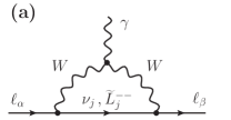
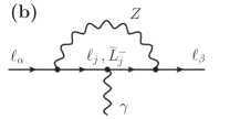
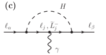
Figure 1: Lowest-order diagrams that are relevant for the amplitude calculations of LFV decays ($\ell_{\alpha}\rightarrow\ell_{\beta}\gamma$) and anomalous magnetic moments of SM leptons (when $\alpha=\beta$) in the unitary gauge. Subscript $j$ denotes the flavor of the internal leptons, and is summed over in the computation. (a) The case mediated by $\nu_{j}$ corresponds to the usual diagram studied in standard electroweak theory, while the $\widetilde{L}^{--}_{j}$ diagram comes from the new interactions; (b) & (c) are new contributing diagrams involving the $Z$ boson and physical Higgs, $H$, respectively.

Applying the modified coupling matrices given in (19) to (21), we can easily relate the new physics parameter $\lambda_{\alpha\beta}$ to these LFV processes. When explicitly computing the diagrams in Fig. 1 in the unitary gauge, our strategy is to perform the calculations in terms of the generalized renormalizable ($R_{\xi}$) gauge Fujikawa:1972fe , and subsequently, taking the limit $\xi\rightarrow\infty$ to obtain the desired results. Moreover, we will work exclusively in the $m_{\ell_{j}}\ll M_{W,Z,H}$ and $m_{\beta}\ll 1$ limits (where $m_{\ell_{j}}$ and $m_{\beta}$ represent the masses of the internal $j$-flavor and the final state SM lepton respectively), dropping any sub-leading order terms in the process. In these limits, one also finds that amplitudes $A$ and $B$ become identical and we may simply pick out the coefficients associated with the $\overline{u}_{\beta}(1\pm\gamma_{5})(2p\cdot\varepsilon)u_{\alpha}$ components in (50), where $p$ denotes the momentum of $\ell_{\beta}$, to get our final expressions.

After the dust has settled and to leading order in $\lambda$, we obtain the following expressions for the amplitudes of the various one-loop contributions (superscripts and subscripts denote the type of internal leptons and bosons involved respectively):

$$A_{W}^{\nu} =\frac{iG_{F}m_{\alpha}e}{8\pi^{2}\sqrt{2}}\sum_{j}\frac{m_{\nu_{j}}^{2}}{4M_{W}^{2}}\left(U_{\nu}\right)_{\beta j}\left(U_{\nu}^{\dagger}\right)_{j\alpha}\simeq 0\,,$$ (51)

$$A_{W}^{\widetilde{L}^{--}} =\frac{iG_{F}m_{\alpha}e}{8\pi^{2}\sqrt{2}}\sum_{j}\frac{v^{2}}{2}\left(\widetilde{Y}\widetilde{M}^{-1}\right)_{\beta j}\left(\widetilde{M}^{-1}\widetilde{Y}^{\dagger}\right)_{j\alpha}\left[f_{1}(w_{j})+f_{2}(w_{j})\right]\,,\qquad w_{j}\equiv\widetilde{M}_{j}^{2}/M_{W}^{2}\;,$$ (52)

$$A_{Z}^{\ell} =\frac{iG_{F}m_{\alpha}e}{8\pi^{2}\sqrt{2}}\,\left(1-\frac{8}{3}\sin^{2}\theta_{w}+\frac{4}{3}\sin^{4}\theta_{w}\right)\lambda_{\beta\alpha}\;,$$ (53)

$$A_{Z}^{\widetilde{L}^{-}} =\frac{iG_{F}m_{\alpha}e}{8\pi^{2}\sqrt{2}}\sum_{j}\frac{v^{2}}{2}\left(\widetilde{Y}\widetilde{M}^{-1}\right)_{\beta j}\left(\widetilde{M}^{-1}\widetilde{Y}^{\dagger}\right)_{j\alpha}\left[f_{3A}(z_{j})+f_{3B}(z_{j})+2f_{4}(z_{j})+3f_{5}(z_{j})\right]\,,\quad z_{j}\equiv\widetilde{M}_{j}^{2}/M_{Z}^{2}\;,$$ (54)

$$A_{H}^{\ell} =\frac{iG_{F}m_{\alpha}e}{8\pi^{2}\sqrt{2}}\;\mathcal{O}\left(\frac{m_{\alpha}^{2}}{M_{H}^{2}}\ln\left[\frac{m_{\alpha}^{2}}{M_{H}^{2}}\right]\right)\lambda_{\beta\alpha}\simeq 0\;,$$ (55)

$$A_{H}^{\widetilde{L}^{-}} =\frac{iG_{F}m_{\alpha}e}{8\pi^{2}\sqrt{2}}\sum_{j}\frac{v^{2}}{2}\left(\widetilde{Y}\right)_{\beta j}\widetilde{M}_{j}^{-2}\left(\widetilde{Y}^{\dagger}\right)_{j\alpha}\left[2f_{5}(h_{j})+f_{6}(h_{j})\right]\,,\qquad h_{j}\equiv\widetilde{M}_{j}^{2}/M_{H}^{2}\;,$$ (56)

with

$$f_{1}(x) =\frac{-10+43x-78x^{2}+49x^{3}-4x^{4}-18x^{3}\ln x}{12(x-1)^{4}}\;,$$ (57)

$$f_{2}(x) =\frac{4-15x+12x^{2}-x^{3}-6x^{2}\ln x}{2(x-1)^{3}}\;,$$ (58)

$$f_{3A}(x) =\frac{4-9x+5x^{3}-6x(2x-1)\ln x}{12(x-1)^{4}}\;,$$ (59)

$$f_{3B}(x) =\frac{2(1-x^{2}+2x\ln x)}{(x-1)^{3}}\;,$$ (60)

$$f_{4}(x) =\frac{-11x+18x^{2}-9x^{3}+2x^{4}-6x\ln x}{48(x-1)^{4}}\;,$$ (61)

$$f_{5}(x) =\frac{-3x+4x^{2}-x^{3}-2x\ln x}{8(x-1)^{3}}\;,$$ (62)

$$f_{6}(x) =\frac{-2x-3x^{2}+6x^{3}-x^{4}-6x^{2}\ln x}{24(x-1)^{4}}\;.$$ (63)

In the above, $m_{\nu_{j}}$, $m_{\alpha}$ and $\widetilde{M}_{j}$ denote, respectively, the masses of the $j$-flavor neutrino, the decaying SM lepton $\ell_{\alpha}$ and the exotic $\widetilde{L}$ particle. Note that (51) is nothing but the contribution due to the SM electroweak interactions when neutrinos carry a nonzero mass. It is well-known that the size of this is negligible Cheng:1985bj ; mu2eg_SM ; Bilenky:1987ty as it receives a $m_{\nu_{j}}^{2}/M_{W}^{2}$ suppression.

With these amplitudes and the general formula for the total decay rate,

$$\Gamma(\ell_{\alpha}\rightarrow\ell_{\beta}\gamma)=\frac{m_{\alpha}^{3}}{4\pi}\left|A_{W}^{\nu}+A_{W}^{\widetilde{L}^{--}}+A_{Z}^{\ell}+A_{Z}^{\widetilde{L}^{-}}+A_{H}^{\ell}+A_{H}^{\widetilde{L}^{-}}\right|^{2}\;,$$ (64)

we obtain the branching ratio (after dropping $A_{W}^{\nu},A_{H}^{\ell}\simeq 0$)

$$\text{Br}(\ell_{\alpha}\rightarrow\ell_{\beta}\gamma) =\frac{3\alpha_{e}}{2\pi}\left|\left(1-\frac{8}{3}\sin^{2}\theta_{w}+\frac{4}{3}\sin^{4}\theta_{w}\right)\lambda_{\beta\alpha}+\sum_{j}\frac{v^{2}}{2}\left(\widetilde{Y}\right)_{\beta j}\widetilde{M}_{j}^{-2}\left(\widetilde{Y}^{\dagger}\right)_{j\alpha}\left[\phantom{\frac{}{}}f_{1}(w_{j})+f_{2}(w_{j})\right.\right.$$

$$\qquad\qquad\qquad\left.\left.+f_{3A}(z_{j})+f_{3B}(z_{j})+f_{4}(z_{j})+3f_{5}(z_{j})+2f_{5}(h_{j})+f_{6}(h_{j})\phantom{\frac{}{}}\right]\phantom{\sum_{j}}\right|^{2}\text{Br}(\ell_{\alpha}\rightarrow\ell_{\beta}\nu_{\alpha}\overline{\nu}_{\beta})\;,$$ (65)

where $\alpha_{e}$ is the fine-structure constant. Taking $\widetilde{M}_{j}\simeq\mathcal{O}\left(100\right)$ GeV (this is around the global lower bound for heavy charged leptons from current experiments Nakamura:2010zzi ) for all $j$, and assuming the Higgs mass, $M_{H}$, is about 114 GeV Barate:2003sz , the experimental limits Nakamura:2010zzi on $\text{Br}(\mu\rightarrow e\gamma)$, $\text{Br}(\tau\rightarrow e\gamma)$ and $\text{Br}(\tau\rightarrow\mu\gamma)$ then lead to

$$|\lambda_{e\mu}|<2.4\times 10^{-5}\;,$$ (66)

$$|\lambda_{e\tau}|<3.0\times 10^{-3}\;,$$ (67)

$$|\lambda_{\mu\tau}|<3.5\times 10^{-3}\;.$$ (68)

Although these bounds are weaker than those displayed in (43) to (45), the derived expressions above will be very useful when the expected improvement in the experimental bounds are realized in the near future (besides the upper limits, (67) and (68), are only marginally bigger than their counterparts). Currently, the MEG experiment exp_MEG located at Paul Scherrer Institute (PSI) is planning to reach a sensitivity of $\mathcal{O}\left(10^{-13}\right)$ for the $\mu\rightarrow e\gamma$ branching ratio, which is a significant improvement compare to the current limit of $\text{Br}(\mu\rightarrow e\gamma)$ $<1.2\times 10^{-11}$ Brooks:1999pu . In addition, the Super KEKB project exp_SuperB will provide an excellent platform for investigating LFV $\tau$ decays at an unprecedented precision. As a result, the bounds on $\tau\rightarrow e\gamma$ and $\tau\rightarrow\mu\gamma$ are also expected to tighten, providing a stronger constraint for all off-diagonal couplings $\lambda_{\alpha\beta}$ than presented here.

VI $\mu$-$e$ conversion in atomic nuclei

Muon-to-electron conversion in muonic atoms provides another excellent testing field for tree-level FCNC. This is because coherent contribution of all nucleons in the nucleus can enhance the experimental signals, and hence the $\mu$-$e$-$Z$ vertex may be probed at great precision. Given that this is the same vertex as appeared in the loop graphs in Fig 1b, the test for $\mu$-$e$ conversion, therefore, plays a complementary role to the investigation of $\mu\rightarrow e\gamma$ in the probe for physics beyond the SM as the two processes are induced differently.

In what follows, we shall assume that the only contribution to the $\mu$-$e$ conversion rate in our setup comes from exchanges with the $Z$ bosons. This approximation is sensible because the cases mediated by the photon and the Higgs are suppressed by loop effects and $M_{H}^{-1}$ respectively. So, assuming only SM interactions operate in the quark sector, we obtain the following effective interaction Lagrangian for the $\mu$-$e$ transition (after integrating out $M_{Z}$):

$$\mathcal{L}^{\text{eff}}_{\mu\rightarrow e} =\sqrt{2}\,G_{F}\overline{\ell}_{e}\gamma^{\nu}(k_{V}-k_{A}\gamma_{5})\ell_{\mu}\left[\overline{q}_{u}\gamma_{\nu}(v_{u}+a_{u}\gamma_{5})q_{u}+\overline{q}_{d}\gamma_{\nu}(v_{d}+a_{d}\gamma_{5})q_{d}\right]\;,$$ (69)

where $q_{u,d}$ denotes the $u,d$-quark field while

$$k_{V}=-k_{A}=\left(\frac{1}{2}-\sin^{2}\theta_{w}\right)\lambda_{e\mu}\;,\quad a_{u}=-a_{d}=-\frac{1}{2}\;,\quad v_{u}=\frac{1}{2}-\frac{4}{3}\sin^{2}\theta_{w}\;,\quad v_{d}=-\frac{1}{2}+\frac{2}{3}\sin^{2}\theta_{w}\;.$$ (70)

Appealing to the general result obtained from FCNC analysis with massive gauge bosons in Bernabeu:1993ta , the branching ratio for $\mu$-$e$ conversion in nuclei (for nuclei with less than about 100 nucleons) is found to be

$$B_{\mu\rightarrow e}\simeq\frac{G_{F}^{2}\,\alpha_{e}^{3}\,m_{\mu}^{3}\,p_{e}^{\prime}\,E_{e}^{\prime}}{\pi^{2}\,\Gamma_{\text{cap}}^{\mathcal{A}}}\left|F(q^{\prime 2})\right|^{2}\left(k_{V}^{2}+k_{A}^{2}\right)\frac{\mathcal{Z}_{\text{eff}}^{4}\,\hat{Q}^{2}}{\mathcal{Z}}\;,$$ (71)

where $p_{e}^{\prime}$ ($E_{e}^{\prime}$) is the momentum (energy) of the electron, $\Gamma_{\text{cap}}^{\mathcal{A}}$ represents the total nuclear muon capture rate for element $\mathcal{A}$, and $\mathcal{Z}$ ($\mathcal{Z}_{\text{eff}}$) is the (effective) atomic number of the element under investigation. In (71), $F(q^{\prime 2})$ is the nuclear form factor which may be measured from electron scattering experiments 11of_ref22 while

$$\hat{Q}=(2\mathcal{Z}+\mathcal{N})\,v_{u}+(\mathcal{Z}+2\mathcal{N})\,v_{d}\;,$$ (72)

with $\mathcal{N}$ denoting the number of neutrons in the nuclei.

Given that one of the best upper limit on the $\mu$-$e$ conversion branching ratio is obtained from measurements with titanium-48 (${}^{48}_{22}\text{Ti}$) in the SINDRUM II experiments Dohmen:1993mp :

$$B_{\mu\rightarrow e}^{\text{exp}}\equiv\frac{\Gamma(\mu^{-}\,\text{Ti}\rightarrow e^{-}\,\text{Ti})}{\Gamma_{\text{cap}}^{\text{Ti}}}<4.3\times 10^{-12}\;,$$ (73)

we shall use the parameters for element ${}^{48}_{22}\text{Ti}$ in (71) to deduce our bound. Following the approximation as applied in Bernabeu:1993ta , we take $p_{e}^{\prime}\simeq E_{e}^{\prime}\simeq m_{\mu}$, and $F(q^{\prime 2}\simeq-m_{\mu}^{2})\simeq 0.54$. In addition, we have $\mathcal{Z}_{\text{eff}}\simeq 17.6$ for ${}^{48}_{22}\text{Ti}$ Zeff and $\Gamma_{\text{cap}}^{\mathcal{A}}\equiv\Gamma_{\text{cap}}^{\text{Ti}}\simeq 2.59\times 10^{6}$ s^-1 Suzuki:1987jf . Hence, (71) and (73) combine to give

$$|\lambda_{e\mu}|<1.9\times 10^{-6}\;.$$ (74)

As hinted earlier, the bound displayed in (74) is indeed the most stringent one on $|\lambda_{e\mu}|$. Moreover, given that new $\mu$-$e$ experiments are being planned, respectively, at J-PARC and Fermilab by the COMET (and PRISM/PRIME) exp_COMET and Mu2e exp_mu2e collaborations, this bound is expected to be further strengthened in the near future.

VII Global fit on the elements of $\lambda$ and some consequences

In this section, we bring together all the results obtained thus far and perform a global analysis on the elements of the $\lambda$ matrix, which are key to determining the new physics effects from the doublet leptons, $\widetilde{L}$. For convenience, a summary of all constraints derived in the previous four sections are collected in Table 2.

parameter(s)	process	limit on BR	constraint on $\lambda$’s
$\lambda_{ee}$	$Z\rightarrow e^{-}e^{+}$	$3.363\pm 0.004\times 10^{-2}$
$\lambda_{\mu\mu}$	$Z\rightarrow\mu^{-}\mu^{+}$	$3.366\pm 0.007\times 10^{-2}$	$\;\lesssim 10^{-3}\;$
$\lambda_{\tau\tau}$	$Z\rightarrow\tau^{-}\tau^{+}$	$3.369\pm 0.008\times 10^{-2}$
$|\lambda_{e\mu}|$	$Z\rightarrow e^{\pm}\mu^{\mp}$ $\mu^{-}\rightarrow e^{-}e^{-}e^{+}$ $\mu\rightarrow e\gamma$ $\mu$-$e$ conversion	$<1.7\times 10^{-6}$ $<1.0\times 10^{-12}$ $<1.2\times 10^{-11}$ $<4.3\times 10^{-12}$ (Ti)	$<6.6\times 10^{-3}$ $<4.7\times 10^{-6}$ $<2.4\times 10^{-5}$ $<1.9\times 10^{-6}$
$|\lambda_{e\tau}|$	$Z\rightarrow e^{\pm}\tau^{\mp}$ $\tau^{-}\rightarrow e^{-}e^{-}e^{+}$ $\tau^{-}\rightarrow e^{-}\mu^{-}\mu^{+}$ $\tau\rightarrow e\gamma$	$<9.8\times 10^{-6}$ $<3.6\times 10^{-8}$ $<3.7\times 10^{-8}$ $<3.3\times 10^{-8}$	$<1.6\times 10^{-2}$ $<2.1\times 10^{-3}$ $<3.4\times 10^{-3}$ $<3.0\times 10^{-3}$
$|\lambda_{\mu\tau}|$	$Z\rightarrow\mu^{\pm}\tau^{\mp}$ $\tau^{-}\rightarrow\mu^{-}\mu^{-}\mu^{+}$ $\tau^{-}\rightarrow\mu^{-}e^{-}e^{+}$ $\tau\rightarrow\mu\gamma$	$<1.2\times 10^{-5}$ $<3.2\times 10^{-8}$ $<2.7\times 10^{-8}$ $<4.4\times 10^{-8}$	$<1.8\times 10^{-2}$ $<2.0\times 10^{-3}$ $<2.2\times 10^{-3}$ $<3.5\times 10^{-3}$
$|\lambda_{\mu e}||\lambda_{\mu\tau}|$	$\tau\rightarrow e^{+}\mu^{-}\mu^{-}$	$<2.3\times 10^{-8}$	$<3.6\times 10^{-3}$
$|\lambda_{e\mu}||\lambda_{e\tau}|$	$\tau\rightarrow\mu^{+}e^{-}e^{-}$	$<2.0\times 10^{-8}$	$<3.3\times 10^{-3}$

Table 2: A collection of all constraints on the elements of $\lambda\equiv v^{2}\widetilde{Y}\widetilde{M}^{-2}\widetilde{Y}^{\dagger}/2$ from processes studied in the previous four sections.

Studying the results listed in Table 2 and recalling that $|\lambda_{\alpha\beta}|=|\lambda_{\beta\alpha}|$, it is not difficult to obtain the following overall fit for the elements of $\lambda$:

$$\begin{pmatrix}|\lambda_{ee}|&|\lambda_{e\mu}|&|\lambda_{e\tau}|\\ |\lambda_{\mu e}|&|\lambda_{\mu\mu}|&|\lambda_{\mu\tau}|\\ |\lambda_{\tau e}|&|\lambda_{\tau\mu}|&|\lambda_{\tau\tau}|\end{pmatrix}\lesssim\begin{pmatrix}10^{-3}&1.9\times 10^{-6}&2.1\times 10^{-3}\\ 1.9\times 10^{-6}&10^{-3}&2.0\times 10^{-3}\\ 2.1\times 10^{-3}&2.0\times 10^{-3}&10^{-3}\end{pmatrix}\;.$$ (75)

Result (75) is one of our major results in this work. Using the definition, $\lambda\equiv v^{2}\widetilde{Y}\widetilde{M}^{-2}\widetilde{Y}^{\dagger}/2$, and taking $\widetilde{M}\simeq\mathcal{O}\left(100\right)$ GeV (for all flavors), a rough estimate of the size for the new couplings $|\widetilde{Y}_{ij}|$ may be obtained:

$$\left|\widetilde{Y}_{ij}\right|\lesssim\mathcal{O}\left(10^{-2}\right)\text{ to }\mathcal{O}\left(10^{-3}\right)\;,\qquad\text{for all }i,j\;.$$ (76)

If the exotic particle mass $\widetilde{M}$ is heavier than the value used above, the upper limit for $|\widetilde{Y}_{ij}|$ will be increased.

Furthermore, if we assume that the new flavor changing physics due to the presence of these exotic $\widetilde{L}$’s are the only source of LFV, one may derive model-specific bounds on the various processes predicted by this model from studying the ratio between the different branching ratios:

$$\text{Br}(Z\rightarrow e^{\pm}\mu^{\mp}) \simeq 4.8\times 10^{-1}\;\text{Br}(\mu\text{-}e\,\text{conversion in Ti})\;,$$

$$\text{Br}(\mu^{-}\rightarrow e^{-}e^{-}e^{+}) \simeq 3.9\times 10^{-2}\;\text{Br}(\mu\text{-}e\,\text{conversion in Ti})\;,$$

$$\text{Br}(\mu\rightarrow e\gamma) \simeq 1.9\times 10^{-2}\;\text{Br}(\mu\text{-}e\,\text{conversion in Ti})\;,$$ (77)

for the processes involving $|\lambda_{e\mu}|^{2}$. Whereas for $|\lambda_{e\tau}|^{2}$ and $|\lambda_{\mu\tau}|^{2}$, one may write

$$\text{Br}(Z\rightarrow e^{\pm}\tau^{\mp}) \simeq 7.0\times 10^{1}\;\text{Br}(\tau^{-}\rightarrow e^{-}e^{-}e^{+})\;,$$

$$\text{Br}(\tau^{-}\rightarrow e^{-}\mu^{-}\mu^{+}) \simeq 6.5\times 10^{-1}\;\text{Br}(\tau^{-}\rightarrow e^{-}e^{-}e^{+})\;,$$

$$\text{Br}(\tau\rightarrow e\gamma) \simeq 4.6\times 10^{-1}\;\text{Br}(\tau^{-}\rightarrow e^{-}e^{-}e^{+})\;,$$ (78)

and

$$\text{Br}(Z\rightarrow\mu^{\pm}\tau^{\mp}) \simeq 7.1\times 10^{1}\;\text{Br}(\tau^{-}\rightarrow\mu^{-}\mu^{-}\mu^{+})\;,$$

$$\text{Br}(\tau^{-}\rightarrow\mu^{-}e^{-}e^{+}) \simeq 6.9\times 10^{-1}\;\text{Br}(\tau^{-}\rightarrow\mu^{-}\mu^{-}\mu^{+})\;,$$

$$\text{Br}(\tau\rightarrow\mu\gamma) \simeq 4.6\times 10^{-1}\;\text{Br}(\tau^{-}\rightarrow\mu^{-}\mu^{-}\mu^{+})\;,$$ (79)

respectively. Whenever required in the above, we have used $\widetilde{M}\simeq\mathcal{O}\left(100\right)$ GeV Nakamura:2010zzi . The main point is that we can translate these into model-specific bounds for certain LFV processes which may be used to falsify this theory. For instance, applying the experimental limits on the right-hand side of (77) implies that this model demands $\text{Br}(\mu\rightarrow e\gamma)\lesssim 8.2\times 10^{-14}$. Observe that this is a couple of orders stronger than the limit set by current experiments. As a result, a future detection of this LFV process above this rate will invalidate the predictions of this minimal extension to the SM, and point to the existence of other new physics in the lepton sector. Similar conclusions may also be drawn from other processes displayed above.

VIII Contribution to lepton anomalous magnetic moment

While in Dirac theory the gyromagnetic ratio of a spin-1/2 particle is predicted to have a value of $\tilde{g}^{\text{dirac}}=2$, it is well-known that quantum field theory gives a correction to this number via loop effects. The deviation from the Dirac result of 2 is usually parameterized by the dimensionless quantity ($\alpha$ denotes the flavor)

$$a_{\alpha}\equiv\frac{\tilde{g}_{\alpha}-2}{2}\;,\quad\text{where $\tilde{g}_{\alpha}$ is the actual value of the gyromagnetic ratio,}$$ (80)

known as the anomalous magnetic moment. It is related to the lepton magnetic dipole moment $\vec{\mu}_{\alpha}=-e(1+a_{\alpha})/2m_{\alpha}\,\vec{s}$, where $\vec{s}$ is the unit spin vector. In terms of the parameters from quantum field theory, $a_{\alpha}\equiv F_{2}(q^{2}=0)$, when the form factor expansion for a general lepton-photon amplitude is written as

$$T(\ell_{\alpha}\rightarrow\ell_{\alpha}^{\prime}\gamma)=-ie\,\overline{u}_{\alpha}^{\prime}\left[F_{1}(q^{2})\gamma_{\rho}+\frac{F_{2}(q^{2})}{2m_{\alpha}}\,i\sigma_{\rho\nu}\,q^{\nu}+\frac{F_{3}(q^{2})}{2m_{\alpha}}\,\sigma_{\rho\nu}\gamma_{5}\,q^{\nu}+\cdots\right]\varepsilon^{\rho}u_{\alpha}\;,\quad e>0\;,$$ (81)

where $q^{\nu}$ is again the photon momentum (see (50) for notations). Therefore, the precise contribution to $a_{\alpha}$ from the SM (and indeed any other theories) can be calculated by considering all the relevant loop diagrams for the $F_{2}(0)$-term.

While the anomalous magnetic moment for the electron, muon and tauon can all be very important in their own rights, given the present experimental and theoretical development, $a_{\mu}$ is the most interesting observable to examine. This is because when combining the fact that significant contributions to the overall predicted $a_{\mu}$ value come from every major sector (QED, electroweak, hadronic) of the SM g-2_review1 ; mg-2_SM with the ability to experimentally measure $a_{\mu}$ to extremely high accuracy mg-2_exp1 ; mg-2_exp2 , the SM as a whole can be scrutinized, and any discrepancies between theory and experiment would be a strong indication of new physics. On the other hand, although $a_{e}$ have been measured to extraordinary precision (hence providing a very stringent test on QED and the value of the fine-structure constant $\alpha_{e}$ eg-2_exp ; eg-2_fineS ), its low sensitivity to the contributions from strong and electroweak processes means that any hypothetical modifications to these sectors (due to new physics) would not be easily detectable. As far as $a_{\tau}$ is concerned, even though its much heavier mass would in theory imply better sensitivity to any new physics than $a_{\mu}$, its usefulness has been limited by the relatively poor experimental bounds. In fact, the best current limits set by the DELPHI experiments DELPHI are still too coarse to even check the first significant figure of $a_{\tau}$ from theoretical calculations.

Currently, the experimental values for $a_{e}$ eg-2_exp , $a_{\mu}$ mg-2_exp2 and $a_{\tau}$ DELPHI are given by

$$a_{e}^{\text{Exp}} =115~{}965~{}218~{}073(28)\times 10^{-14}\;,$$ (82)

$$a_{\mu}^{\text{Exp}} =116~{}592~{}089(63)\times 10^{-11}\;,$$ (83)

$$a_{\tau}^{\text{Exp}} =\begin{cases}\;<1.3\times 10^{-2}\;,\\ \;>-5.2\times 10^{-2}\;.\end{cases}$$ (84)

Focusing on the muon case, one finds that the discrepancy between experiment and the SM estimate is about 4.0$\sigma$ mg-2_SM :

$$\Delta a_{\mu}=a_{\mu}^{\text{Exp}}-a_{\mu}^{\text{SM}}=316(79)\times 10^{-11}\;.$$ (85)

If this difference is real (rather than caused by incorrect leading-order hadronic approximation), then there must be some new physics at play. In the following, we investigate whether the presence of the exotic doublets can affect this quantity in a significant way.

Calculating the anomalous magnetic moment using the modified electroweak couplings of (19) to (21) is in fact analogous to the computation for LFV $\ell_{\alpha}\rightarrow\ell_{\beta}\gamma$ done in Sec. V. The only differences are that $\alpha=\beta$ here and we do not take the zero mass limit for the final state lepton. Otherwise, the three main types of one-loop diagrams we need to consider are as depicted in Fig. 1. Working in the unitary gauge again, and noting that for the magnetic moment, the part associated with $\gamma_{5}$ in the general amplitude

$$T(\ell_{\alpha}\rightarrow\ell_{\alpha}^{\prime}\gamma)=\overline{u}_{\alpha}^{\prime}\,(C+D\gamma_{5})\,i\sigma_{\rho\nu}q^{\nu}\varepsilon^{\rho}u_{\alpha}\;,$$ (86)

is not needed. Hence, in the computation, we pick out the terms that are proportional to $\overline{u}_{\alpha}^{\prime}(2p\cdot\varepsilon)u_{\alpha}$, where $p$ is again the momentum of the incoming $\ell_{\alpha}$. Employing a similar notation system as before, the amplitudes of the one-loop diagrams from Fig. 1 for the case $\alpha=\beta$ are given by (to leading order)

$$C_{W}^{\nu} =\frac{iG_{F}m_{\alpha}e}{8\pi^{2}\sqrt{2}}\left(-\frac{5}{3}\right),$$ (87)

$$C_{W}^{\widetilde{L}^{--}} =\frac{iG_{F}m_{\alpha}e}{8\pi^{2}\sqrt{2}}\sum_{j}\frac{v^{2}}{2}\left(\widetilde{Y}\widetilde{M}^{-1}\right)_{\alpha j}\left(\widetilde{M}^{-1}\widetilde{Y}^{\dagger}\right)_{j\alpha}\left[f_{7}(w_{j})+3f_{8}(w_{j})+f_{9}(w_{j})-1\right],\quad w_{j}\equiv\widetilde{M}_{j}^{2}/M_{W}^{2}\;,$$ (88)

$$C_{Z}^{\ell} =\frac{iG_{F}m_{\alpha}e}{8\pi^{2}\sqrt{2}}\left(\frac{2}{3}(1+2\sin^{2}\theta_{w}-4\sin^{4}\theta_{w})+\frac{2\lambda_{\alpha\alpha}}{3}(4\sin^{4}\theta_{w}-8\sin^{2}\theta_{w}+3)\right),$$ (89)

$$C_{Z}^{\widetilde{L}^{-}} =\frac{iG_{F}m_{\alpha}e}{8\pi^{2}\sqrt{2}}\sum_{j}\frac{v^{2}}{2}\left(\widetilde{Y}\widetilde{M}^{-1}\right)_{\alpha j}\left(\widetilde{M}^{-1}\widetilde{Y}^{\dagger}\right)_{j\alpha}\left[2f_{3A}(z_{j})+2f_{3B}(z_{j})+f_{4}(z_{j})+2f_{5}(z_{j})\right],\quad z_{j}\equiv\widetilde{M}_{j}^{2}/M_{Z}^{2}\;,$$ (90)

$$C_{H}^{\ell} =\frac{iG_{F}m_{\alpha}e}{8\pi^{2}\sqrt{2}}\,(1-4\lambda_{\alpha\alpha})\;\mathcal{O}\left(m_{\alpha}^{2}/M_{H}^{2}\right)\simeq 0\;,$$ (91)

$$C_{H}^{\widetilde{L}^{-}} =\frac{iG_{F}m_{\alpha}e}{8\pi^{2}\sqrt{2}}\sum_{j}\frac{v^{2}}{2}\,\widetilde{Y}_{\alpha j}\widetilde{M}^{-2}_{j}\widetilde{Y}^{\dagger}_{j\alpha}\left[4f_{5}(h_{j})+2f_{6}(h_{j})\right]\,,\quad h_{j}\equiv\widetilde{M}_{j}^{2}/M_{H}^{2}\;,$$ (92)

where $f_{3A}(x)$ to $f_{6}(x)$ are given in (59) to (63) and

$$f_{7}(x) =\frac{7-33x+57x^{2}-31x^{3}+6x^{2}(3x-1)\ln x}{6(x-1)^{4}}\;,$$ (93)

$$f_{8}(x) =\frac{1-4x+3x^{2}-2x^{2}\ln x}{(x-1)^{3}}\;,$$ (94)

$$f_{9}(x) =\frac{3-10x+21x^{2}-18x^{3}+4x^{4}+6x^{2}\ln x}{6(x-1)^{4}}\;.$$ (95)

Comparing (86) with the form factor expansion of (81), the anomalous magnetic moment can be written in terms of the amplitudes computed above:

$$a_{\alpha}\equiv F_{2}(0)=-\frac{2m_{\alpha}}{ie}\left(C_{W}^{\nu}+C_{W}^{\widetilde{L}^{--}}+C_{Z}^{\ell}+C_{Z}^{\widetilde{L}^{-}}+C_{H}^{\ell}+C_{H}^{\widetilde{L}^{-}}\right)\;.$$ (96)

Note that the result given in (96) contains the usual SM electroweak component of $a_{\alpha}$, as well as the contribution induced by the new physics. Examining our results, we see that the terms which are not proportional to $\lambda_{\alpha\alpha}$ in (87) and (89) sum up to give the usual prediction of the anomalous magnetic moment from the SM Fujikawa:1972fe . Removing this component from (96) and using the values for $\lambda_{\alpha\alpha}$ given in Table 2, we obtain the following estimate for the anomalous magnetic moments coming from the new physics associated with the exotic $\widetilde{L}$ particles:

$$\Delta a_{e}^{\widetilde{L}} \simeq 6.6\times 10^{-16}\;,$$ (97)

$$\Delta a_{\mu}^{\widetilde{L}} \simeq 3.2\times 10^{-11}\;,$$ (98)

$$\Delta a_{\tau}^{\widetilde{L}} \simeq 1.1\times 10^{-8}\;,$$ (99)

where we have again assumed $\widetilde{M}_{j}\simeq\mathcal{O}\left(100\right)$ GeV and $M_{H}\simeq 114$ GeV. Looking at the results (97) to (99), we see that these contributions are at least one order of magnitude less than the experimental errors given for the quantities listed in (82) to (84). Therefore, these exotic $\widetilde{L}$’s cannot help to explain the muon $g-2$ anomaly nor can their effects be easily distinguishable from the SM components in these experiments.

IX Comments on collider signatures

If the exotic doublets $\widetilde{L}$ do exist, it would give rise to collider signals which may be detectable at the LHC. Given that the exotic mass $\widetilde{M}$ is not too massive and assuming some favorable conditions are met, such signatures can be quite distinctive as pointed out recently in DelNobile:2009st . In this section, we summarize some of the key features one can expect from the presence of these exotic particles.

To make the situation more clear-cut, let suppose Yukawa couplings $\widetilde{Y}$ are small enough such that $\widetilde{L}$ production is predominantly mediated by SM gauge interactions. The relevant production mechanisms at the partonic level are then given by:

$$q\overline{q}\rightarrow\gamma,Z\rightarrow\widetilde{L}^{-}\widetilde{L}^{+}\;,\;\widetilde{L}^{--}\widetilde{L}^{++}\quad;\quad u\overline{d}\rightarrow W^{+}\rightarrow\widetilde{L}^{-}\widetilde{L}^{++}\;.$$ (100)

With the planned energy of $\sqrt{s}=14$ TeV and luminosity at $300\text{ fb}^{-1}\text{yr}^{-1}$ at the LHC, it is estimated that the pair production cross-section from $pp$ collisions ranges from $\sigma(pp\rightarrow\widetilde{L}\overline{\widetilde{L}})\simeq$ a few fb for $\widetilde{M}\simeq 500$ GeV to just under $10^{3}$ fb for $\widetilde{M}\simeq$ 200 GeV DelNobile:2009st (assuming no cuts are made). Once produced, the singly and doubly charged exotic leptons may decay into SM particles via the interaction terms depicted in (16) to (18):

$$\widetilde{L}^{-}\rightarrow\ell^{-}Z\;,\;\ell^{-}H\;\;\text{ and }\;\;\widetilde{L}^{--}\rightarrow\ell^{-}W^{-}\;.$$ (101)

Note that the decay mode $\widetilde{L}^{-}\rightarrow\nu W^{-}$ is suppressed. Furthermore, we shall assume that the $\widetilde{Y}$ mediated processes dominate over the electroweak decay $\widetilde{L}^{--}\rightarrow\widetilde{L}^{-}\pi^{-}$, which is, strictly speaking, allowed because of the mass splitting of the doublet components due to quantum corrections Q_split . As a result, we may treat both $\widetilde{L}^{-}$ and $\widetilde{L}^{--}$ on an equal footing. Consequently, we see that the three relevant states from $pp$ collisions ($\widetilde{L}^{-}\widetilde{L}^{+},\widetilde{L}^{--}\widetilde{L}^{++}$ and $\widetilde{L}^{-}\widetilde{L}^{++}$) will lead to a generic $\ell^{+}\ell^{-}XX^{\prime}$ signal, where $XX^{\prime}$ denotes one of $ZZ,HH,ZH,W^{+}W^{-},ZW^{+}$ or $HW^{+}$.

For instance, the case $pp\rightarrow\gamma,Z\rightarrow\widetilde{L}^{--}\widetilde{L}^{++}$ will give rise to a $\ell^{+}W^{+}\ell^{-}W^{-}$ state. Subsequently, the $W$ bosons may decay leptonically or hadronically leading to one of the final states (in order of descending branching fraction): $\ell^{+}\ell^{-}j$, $\ell^{\pm}\ell^{\pm}\not{E}_{T}\ell^{\mp}j$ or $\ell^{+}\ell^{-}\ell^{+}\ell^{-}\not{E}_{T}$, where $\not{E}_{T}$ and $j$ denote the generic missing transverse energy and jets respectively. The relevant SM background processes for this case are $pp\rightarrow t\overline{t}W^{\pm},ZW^{+}W^{-}$ (and perhaps $pp\rightarrow t\overline{t}$). Amongst the three final states, $\ell^{\pm}\ell^{\pm}\not{E}_{T}\ell^{\mp}j$ seems to be the most promising for probing the mass of $\widetilde{M}$ as one may gain information from studying either the two same-sign leptons invariant mass distribution or the invariant mass of the opposite-sign lepton with two jets.

Another interesting case to consider is the $pp\rightarrow W^{+}\rightarrow\widetilde{L}^{-}\widetilde{L}^{++}$ decay chain. Although there are more possibilities for the intermediate state $\ell^{+}\ell^{-}XX^{\prime}$, if one assumes that any subsequent $W$ boson decays only leptonically, then the final signal one gets is either $\ell^{+}\ell^{+}\ell^{-}\not{E}_{T}$ or $\ell^{+}\ell^{+}\ell^{-}\not{E}_{T}j$. The typical SM background one must confront with here is coming from vector boson decays (e.g. from $pp\rightarrow ZW^{+}$). According to a recent analysis in DelNobile:2009st , such channels can provide another promising way to search for these exotic particles. Note, however, that the cleaner state $\ell^{+}\ell^{+}\ell^{-}\not{E}_{T}$ is only possible if $\widetilde{M}$ is low enough.

X Conclusion

Given that the discovery of nonzero neutrino masses demands an extension to the lepton sector, it is natural to ask what might be the simplest ways that new physics can couple to the SM particles. Concentrating on the lepton sector only, we have followed the approach of Chua:2010me and introduced exotic particles into the SM via some “minimal couplings”.

Since many of the exotic particles defined in this way turn out to be equivalent to those studied in other new physics models, we identify that only a couple of possibilities remain unexplored in the literature. While the work of Chua:2010me focused on one of them, in this paper, we have presented the analysis for the last remaining possibility, namely, the exotic doublets $\widetilde{L}$ which couples to the RH charged lepton singlet.

Using a formalism similar to that presented in Chua:2010me , we have defined the key quantity, $\lambda$, which encapsulates the new physics effects caused by the introduction of these exotic $\widetilde{L}$’s. In particular, we note that the off-diagonal entries of this $\lambda$ matrix are the origins of any new FCNC phenomenologies. By invoking the limits from low-energy experiments, constraints are then placed on these entries that control the coupling strength to the exotic $\widetilde{L}$’s. Such an investigation can be quite useful given that these minimally coupled particles may give rise to definite collider signatures at the LHC in the future DelNobile:2009st .

In this paper, the processes considered include leptonic $Z$ decays, LFV $\ell\rightarrow 3\ell$, $\ell\rightarrow\ell^{\prime}\gamma$ decays, as well as $\mu$-$e$ conversion in titanium nuclei. The collection of constraints are displayed in Table 2. We have found that diagonal elements, $|\lambda_{\alpha\alpha}|$, could be as big as $\mathcal{O}\left(10^{-3}\right)$ only, while the most stringent bounds for the off-diagonal values are from LFV $\ell\rightarrow 3\ell$ decays except for $|\lambda_{e\mu}|$ which has its strongest bound coming from the $\mu$-$e$ conversion process. We anticipate that some of these limits will improve significantly when the next generation of experiments have reached their proposed sensitivity.

Finally, the contribution to the lepton anomalous magnetic moment in this model is calculated. The explicit computation of the relevant lowest-order loop graphs shows that any potential contributions is far too small to be detected in experiments at the present time. As a result, introducing this type of exotic doublet of leptons into the SM cannot resolve the muon $g-2$ anomaly.

References

• (1) B. T. Cleveland et al., Nucl. Phys. Proc. Suppl.  38, 47 (1995); Y. Fukuda et al. [Super-Kamiokande Collaboration], Phys. Rev. Lett.  82, 2430 (1999) [arXiv:hep-ex/9812011]; Y. Fukuda et al. [Super-Kamiokande Collaboration], Phys. Rev. Lett.  81, 1562 (1998) [arXiv:hep-ex/9807003]; K. Lande et al., Nucl. Phys. Proc. Suppl.  77, 13 (1999); D. N. Abdurashitov et al. [SAGE Collaboration], Nucl. Phys. Proc. Suppl.  77, 20 (1999); T. A. Kirsten [GALLEX and GNO Collaborations], Nucl. Phys. Proc. Suppl.  77, 26 (1999); Y. Fukuda et al. [Super-Kamiokande Collaboration], Phys. Lett. B 436, 33 (1998) [arXiv:hep-ex/9805006]; C. Athanassopoulos et al. [LSND Collaboration], Phys. Rev. C 54, 2685 (1996) [arXiv:nucl-ex/9605001]; C. Athanassopoulos et al. [LSND Collaboration], Phys. Rev. C 58, 2489 (1998) [arXiv:nucl-ex/9706006]; Q. R. Ahmad et al. [SNO Collaboration], Phys. Rev. Lett.  89, 011301 (2002) [arXiv:nucl-ex/0204008]; S. N. Ahmed et al. [SNO Collaboration], Phys. Rev. Lett.  92, 181301 (2004) [arXiv:nucl-ex/0309004]; K. Eguchi et al. [KamLAND Collaboration], Phys. Rev. Lett.  90, 021802 (2003) [arXiv:hep-ex/0212021], P. Adamson et al. [MINOS Collaboration], Phys. Rev. Lett.  103, 261802 (2009) [arXiv:0909.4996 [hep-ex]], arXiv:1007.2791 [hep-ex], A. A. Aguilar-Arevalo et al. [MiniBooNE Collaboration], Phys. Rev. Lett.  103, 061802 (2009) [arXiv:0903.2465 [hep-ex]].
• (2) C. K. Chua and S. S. C. Law, Phys. Rev.  D 83, 055010 (2011) [arXiv:1011.4730 [hep-ph]].
• (3) E. Del Nobile, R. Franceschini, D. Pappadopulo and A. Strumia, Nucl. Phys.  B 826, 217 (2010) [arXiv:0908.1567 [hep-ph]].
• (4) For examples: Y. Grossman, Nucl. Phys.  B 426, 355 (1994) [arXiv:hep-ph/9401311] and references therein, Y. Grossman and Y. Nir, Phys. Lett.  B 313, 126 (1993) [arXiv:hep-ph/9306292], S. Kanemura, T. Kubota and E. Takasugi, Phys. Lett.  B 313, 155 (1993) [arXiv:hep-ph/9303263], Y. Okada, Y. Shimizu and M. Tanaka, Phys. Lett.  B 405, 297 (1997) [arXiv:hep-ph/9704223], A. G. Akeroyd, A. Arhrib and E. M. Naimi, Phys. Lett.  B 490, 119 (2000) [arXiv:hep-ph/0006035], W. Grimus and L. Lavoura, Phys. Lett.  B 546, 86 (2002) [arXiv:hep-ph/0207229], S. Kanemura, T. Ota and K. Tsumura, Phys. Rev.  D 73, 016006 (2006) [arXiv:hep-ph/0505191], E. Lunghi and A. Soni, JHEP 0709, 053 (2007) [arXiv:0707.0212 [hep-ph]].
• (5) M. Aoki, S. Kanemura and O. Seto, Phys. Rev. Lett.  102, 051805 (2009) [arXiv:0807.0361 [hep-ph]], M. Aoki, S. Kanemura and O. Seto, Phys. Rev.  D 80, 033007 (2009) [arXiv:0904.3829 [hep-ph]], K. L. McDonald and B. H. J. McKellar, arXiv:hep-ph/0309270.
• (6) F. Cuypers and S. Davidson, Eur. Phys. J.  C 2, 503 (1998) [arXiv:hep-ph/9609487], Y. Kuno and Y. Okada, Rev. Mod. Phys.  73, 151 (2001) [arXiv:hep-ph/9909265] and references therein.
• (7) For examples (dilepton models): P. H. Frampton and D. Ng, Phys. Rev.  D 45, 4240 (1992), P. H. Frampton, Phys. Rev. Lett.  69, 2889 (1992), P. H. Frampton, D. Ng, T. W. Kephart and T. C. Yuan, Phys. Lett.  B 317, 369 (1993) [arXiv:hep-ph/9210271], A. G. Akeroyd, M. Aoki and H. Sugiyama, Phys. Rev.  D 79, 113010 (2009) [arXiv:0904.3640 [hep-ph]].
• (8) For examples (Zee/Babu or other radiative seesaw models): A. Zee, Nucl. Phys.  B 264, 99 (1986), K. S. Babu, Phys. Lett.  B 203, 132 (1988), S. Kanemura, T. Kasai, G. L. Lin, Y. Okada, J. J. Tseng and C. P. Yuan, Phys. Rev.  D 64, 053007 (2001) [arXiv:hep-ph/0011357], A. Ghosal, Y. Koide and H. Fusaoka, Phys. Rev.  D 64, 053012 (2001) [arXiv:hep-ph/0104104], L. M. Krauss, S. Nasri and M. Trodden, Phys. Rev.  D 67, 085002 (2003) [arXiv:hep-ph/0210389].
• (9) For examples (doubly charged Higgs): T. G. Rizzo, Phys. Rev.  D 25, 1355 (1982) [Addendum-ibid.  D 27, 657 (1983)], M. L. Swartz, Phys. Rev.  D 40, 1521 (1989), A. G. Akeroyd, Phys. Lett.  B 353, 519 (1995), E. J. Chun, K. Y. Lee and S. C. Park, Phys. Lett.  B 566, 142 (2003) [arXiv:hep-ph/0304069], A. G. Akeroyd and M. Aoki, Phys. Rev.  D 72, 035011 (2005) [arXiv:hep-ph/0506176], C. S. Chen, C. Q. Geng and J. N. Ng, Phys. Rev.  D 75, 053004 (2007) [arXiv:hep-ph/0610118], C. S. Chen, C. Q. Geng and D. V. Zhuridov, Phys. Lett.  B 666, 340 (2008) [arXiv:0801.2011 [hep-ph]], P. Fileviez Perez, T. Han, G. Y. Huang, T. Li and K. Wang, Phys. Rev.  D 78, 071301 (2008) [arXiv:0803.3450 [hep-ph]], P. Fileviez Perez, T. Han, G. Y. Huang, T. Li and K. Wang, Phys. Rev.  D 78, 015018 (2008) [arXiv:0805.3536 [hep-ph]], A. G. Akeroyd and C. W. Chiang, Phys. Rev.  D 80, 113010 (2009) [arXiv:0909.4419 [hep-ph]].
• (10) For examples (type II seesaw): G. Senjanovic and R. N. Mohapatra, Phys. Rev.  D 12, 1502 (1975), W. Konetschny and W. Kummer, Phys. Lett.  B 70, 433 (1977), T. P. Cheng and L. F. Li, Phys. Rev.  D 22, 2860 (1980), M. Magg and C. Wetterich, Phys. Lett.  B 94, 61 (1980), J. Schechter and J. W. F. Valle, Phys. Rev.  D 22, 2227 (1980), G. Lazarides, Q. Shafi and C. Wetterich, Nucl. Phys.  B 181, 287 (1981), C. Wetterich, Nucl. Phys.  B 187, 343 (1981), R. N. Mohapatra and G. Senjanovic, Phys. Rev.  D 23, 165 (1981).
• (11) A. Abada, C. Biggio, F. Bonnet, M. B. Gavela and T. Hambye, JHEP 0712, 061 (2007) [arXiv:0707.4058 [hep-ph]].
• (12) C. S. Chen, C. Q. Geng, J. N. Ng and J. M. S. Wu, JHEP 0708, 022 (2007) [arXiv:0706.1964 [hep-ph]], C. S. Chen, C. Q. Geng and D. V. Zhuridov, Eur. Phys. J.  C 60, 119 (2009) [arXiv:0803.1556 [hep-ph]], T. Ohlsson, T. Schwetz and H. Zhang, Phys. Lett.  B 681, 269 (2009) [arXiv:0909.0455 [hep-ph]].
• (13) P. Minkowski, Phys. Lett. B 67, 421 (1977), T. Yanagida, in Workshop on Unified Theories, KEK report 79-18 p.95 (1979), M. Gell-Mann, P. Ramond, R. Slansky, in Supergravity (North Holland, Amsterdam, 1979) eds. P. van Nieuwenhuizen, D. Freedman, p.315., S. L. Glashow, in 1979 Cargese Summer Institute on Quarks and Leptons (Plenum Press, New York, 1980) eds. M. Levy, J.-L. Basdevant, D. Speiser, J. Weyers, R. Gastmans and M. Jacobs, p.687; R. Barbieri, D. V. Nanopoulos, G. Morchio and F. Strocchi, Phys. Lett. B 90, 91 (1980), R. N. Mohapatra and G. Senjanovic, Phys. Rev. Lett.  44, 912 (1980).
• (14) F. del Aguila, J. A. Aguilar-Saavedra and R. Pittau, JHEP 0710, 047 (2007) [arXiv:hep-ph/0703261], A. Atre, T. Han, S. Pascoli and B. Zhang, JHEP 0905, 030 (2009) [arXiv:0901.3589 [hep-ph]] and references therein, S. Kovalenko, Z. Lu and I. Schmidt, Phys. Rev.  D 80, 073014 (2009) [arXiv:0907.2533 [hep-ph]].
• (15) C. Biggio, Phys. Lett.  B 668, 378 (2008) [arXiv:0806.2558 [hep-ph]], W. Chao, arXiv:0806.0889 [hep-ph].
• (16) F. del Aguila and J. A. Aguilar-Saavedra, Phys. Lett.  B 672, 158 (2009) [arXiv:0809.2096 [hep-ph]].
• (17) R. Foot, H. Lew, X. G. He and G. C. Joshi, Z. Phys.  C 44, 441 (1989), E. Ma, Phys. Rev. Lett.  81, 1171 (1998) [arXiv:hep-ph/9805219], E. Ma and D. P. Roy, Nucl. Phys.  B 644, 290 (2002) [arXiv:hep-ph/0206150], B. Bajc and G. Senjanovic, JHEP 0708, 014 (2007) [arXiv:hep-ph/0612029], B. Bajc, M. Nemevsek and G. Senjanovic, Phys. Rev.  D 76, 055011 (2007) [arXiv:hep-ph/0703080], X. G. He and S. Oh, JHEP 0909, 027 (2009) [arXiv:0902.4082 [hep-ph]] and references therein, A. Arhrib, R. Benbrik and C. H. Chen, Phys. Rev.  D 81, 113003 (2010) [arXiv:0903.1553 [hep-ph]],
• (18) A. Abada, C. Biggio, F. Bonnet, M. B. Gavela and T. Hambye, Phys. Rev.  D 78, 033007 (2008) [arXiv:0803.0481 [hep-ph]].
• (19) Some examples: I. F. Ginzburg, I. P. Ivanov and A. Schiller, Phys. Rev.  D 60, 095001 (1999) [arXiv:hep-ph/9802364], P. H. Frampton, P. Q. Hung and M. Sher, Phys. Rept.  330, 263 (2000) [arXiv:hep-ph/9903387], M. Maltoni, V. A. Novikov, L. B. Okun, A. N. Rozanov and M. I. Vysotsky, Phys. Lett.  B 476, 107 (2000) [arXiv:hep-ph/9911535] and references therein, V. A. Novikov, L. B. Okun, A. N. Rozanov and M. I. Vysotsky, Phys. Lett.  B 529, 111 (2002) [arXiv:hep-ph/0111028], T. Cuhadar-Donszelmann, M. Karagoz, V. E. Ozcan, S. Sultansoy and G. Unel, JHEP 0810, 074 (2008) [arXiv:0806.4003 [hep-ph]], O. Antipin, M. Heikinheimo and K. Tuominen, JHEP 0910, 018 (2009) [arXiv:0905.0622 [hep-ph]].
• (20) A. Delgado, C. G. Cely, T. Han and Z. Wang, arXiv:1105.5417 [hep-ph].
• (21) P. H. Frampton and B. H. Lee, Phys. Rev. Lett.  64, 619 (1990), P. H. Frampton and T. W. Kephart, Phys. Rev.  D 42, 3892 (1990), H. Fujii, S. Nakamua and K. Sasaki, Phys. Lett.  B 299, 342 (1993), K. Sasaki, Phys. Lett.  B 308, 297 (1993), P. Ko, in Constraint on dilepton gauge bosons from muonium $\to$ anti-muonium conversion, UMN-TH-1134-93 & TPI-MINN-93-26-T, Jun 7, 1993, M. B. Tully and G. C. Joshi, Phys. Lett.  B 466, 333 (1993) [arXiv:hep-ph/9905552], B. Dutta and S. Nandi, Phys. Lett.  B 340, 86 (1994), K. Sasaki, K. Tokushuku, S. Yamada and Y. Yamazaki, Phys. Lett.  B 345, 495 (1995), K. Horikawa and K. Sasaki, Phys. Rev.  D 53, 560 (1996) [arXiv:hep-ph/9504218], F. Cuypers and M. Raidal, Nucl. Phys.  B 501, 3 (1997) [arXiv:hep-ph/9704224], P. H. Frampton and M. Harada, Phys. Rev.  D 58, 095013 (1998) [arXiv:hep-ph/9711448], N. A. Ky, H. N. Long and D. V. Soa, Phys. Lett.  B 486, 140 (2000) [arXiv:hep-ph/0007010], G. Tavares-Velasco and J. J. Toscano, Phys. Rev.  D 65, 013005 (2002) [arXiv:hep-ph/0108114], E. Ramirez Barreto, Y. A. Coutinho and J. Sa Borges, Braz. J. Phys.  38, 495 (2008), D. Van Soa, P. Van Dong, T. T. Huong and H. N. Long, J. Exp. Theor. Phys.  108, 757 (2009) [arXiv:0805.4456 [hep-ph]].
• (22) E. Witten, Phys. Lett.  B 117, 324 (1982).
• (23) S. Antusch, C. Biggio, E. Fernandez-Martinez, M. B. Gavela and J. Lopez-Pavon, JHEP 0610, 084 (2006) [arXiv:hep-ph/0607020].
• (24) K. Nakamura [Particle Data Group], J. Phys. G 37, 075021 (2010).
• (25) J. Bernabeu, E. Nardi and D. Tommasini, Nucl. Phys.  B 409, 69 (1993) [arXiv:hep-ph/9306251].
• (26) W. J. Marciano, T. Mori and J. M. Roney, Ann. Rev. Nucl. Part. Sci.  58, 315 (2008) and references therein.
• (27) K. Fujikawa, B. W. Lee and A. I. Sanda, Phys. Rev.  D 6, 2923 (1972).
• (28) T. P. Cheng and L. F. Li, Gauge Theory Of Elementary Particle Physics, Oxford, UK: Clarendon (1984) 536p. (Oxford Science Publications).
• (29) M. E. Peskin and D. V. Schroeder, An Introduction To Quantum Field Theory, Reading, USA: Addison-Wesley (1995) 842p.
• (30) T. P. Cheng and L. F. Li, Phys. Rev.  D 16, 1425 (1977), S. T. Petcov, Sov. J. Nucl. Phys.  25, 340 (1977) [Yad. Fiz.  25, 641 (1977)] [Erratum-ibid.  25, 698 (1977)] [Erratum-ibid.  25, 1336 (1977)], W. J. Marciano and A. I. Sanda, Phys. Lett.  B 67, 303 (1977), B. W. Lee and R. E. Shrock, Phys. Rev.  D 16, 1444 (1977).
• (31) S. M. Bilenky and S. T. Petcov, Rev. Mod. Phys.  59, 671 (1987) [Erratum-ibid.  61, 169 (1989)] [Erratum-ibid.  60, 575 (1988)].
• (32) R. Barate et al. [LEP Working Group for Higgs boson searches and ALEPH Collaboration and and], Phys. Lett.  B 565, 61 (2003) [arXiv:hep-ex/0306033].
• (33) S. Ritt [MEG Collaboration], Nucl. Phys. Proc. Suppl.  162, 279 (2006), J. Adam et al. [MEG collaboration], Nucl. Phys.  B 834, 1 (2010) [arXiv:0908.2594 [hep-ex]].
• (34) M. L. Brooks et al. [MEGA Collaboration], Phys. Rev. Lett.  83, 1521 (1999) [arXiv:hep-ex/9905013].
• (35) T. Aushev et al., KEK-REPORT-2009-12, Feb 2010, [arXiv:1002.5012 [hep-ex]] and references therein.
• (36) I. Sick and J. S. Mccarthy, Nucl. Phys.  A 150, 631 (1970), T. W. Donnelly and J. D. Walecka, Ann. Rev. Nucl. Part. Sci.  25, 329 (1975), B. Frois and C. N. Papanicolas, Ann. Rev. Nucl. Part. Sci.  37, 133 (1987) and references therein.
• (37) C. Dohmen et al. [SINDRUM II Collaboration.], Phys. Lett.  B 317, 631 (1993).
• (38) W. H. Bertl et al. [SINDRUM II Collaboration], Eur. Phys. J.  C 47, 337 (2006).
• (39) R. Kitano, M. Koike and Y. Okada, Phys. Rev.  D 66, 096002 (2002) [Erratum-ibid.  D 76, 059902 (2007)] [arXiv:hep-ph/0203110].
• (40) J. C. Sens, Phys. Rev.  113, 679 (1959), H. C. Chiang, E. Oset, T. S. Kosmas, A. Faessler and J. D. Vergados, Nucl. Phys.  A 559, 526 (1993).
• (41) T. Suzuki, D. F. Measday and J. P. Roalsvig, Phys. Rev.  C 35, 2212 (1987).
• (42) A. Sato, PoS NUFACT08, 105 (2008), and talk given at the 4th International Workshop on Nuclear and Particle Physics at J-PARC (NP08), Mito, Ibaraki, Japan, March 2008 (http://nuclpart.kek.jp/NP08/presentations/ muon/pdf/NP08_Muon_Sato.pdf), Y. G. Cui et al. [COMET Collaboration], KEK-2009-10, Jun 2009.
• (43) R. M. Carey et al. [Mu2e Collaboration], FERMILAB-PROPOSAL-0973, Oct 2008, D. Glenzinski, AIP Conf. Proc.  1222, 383 (2010).
• (44) See for examples: M. Davier and W. J. Marciano, Ann. Rev. Nucl. Part. Sci.  54, 115 (2004), M. Passera, J. Phys. G 31, R75 (2005) [arXiv:hep-ph/0411168], M. Passera, Nucl. Phys. Proc. Suppl.  169, 213 (2007) [arXiv:hep-ph/0702027], J. P. Miller, E. de Rafael and B. L. Roberts, Rept. Prog. Phys.  70, 795 (2007) [arXiv:hep-ph/0703049], F. Jegerlehner and A. Nyffeler, Phys. Rept.  477, 1 (2009) [arXiv:0902.3360 [hep-ph]].
• (45) M. Passera, W. J. Marciano and A. Sirlin, arXiv:1001.4528 [hep-ph].
• (46) G. W. Bennett et al. [Muon G-2 Collaboration], Phys. Rev.  D 73, 072003 (2006) [arXiv:hep-ex/0602035], Phys. Rev. Lett.  92, 161802 (2004) [arXiv:hep-ex/0401008], Phys. Rev. Lett.  89, 101804 (2002) [Erratum-ibid.  89, 129903 (2002)] [arXiv:hep-ex/0208001].
• (47) B. L. Roberts, Chin. Phys.  C 34, 741 (2010) [arXiv:1001.2898 [hep-ex]].
• (48) D. Hanneke, S. Fogwell and G. Gabrielse, Phys. Rev. Lett.  100, 120801 (2008) [arXiv:0801.1134 [physics.atom-ph]].
• (49) R. S. Van Dyck, P. B. Schwinberg and H. G. Dehmelt, Phys. Rev. Lett.  59, 26 (1987), G. Gabrielse, D. Hanneke, T. Kinoshita, M. Nio and B. C. Odom, Phys. Rev. Lett.  97, 030802 (2006) [Erratum-ibid.  99, 039902 (2007)].
• (50) J. Abdallah et al. [DELPHI Collaboration], Eur. Phys. J.  C 35, 159 (2004) [arXiv:hep-ex/0406010].
• (51) K. Hagiwara, R. Liao, A. D. Martin, D. Nomura and T. Teubner, arXiv:1105.3149 [hep-ph].
• (52) M. Cirelli, N. Fornengo, A. Strumia, Nucl. Phys.  B753, 178-194 (2006). [hep-ph/0512090]; M. Cirelli, A. Strumia, New J. Phys.  11, 105005 (2009). [arXiv:0903.3381 [hep-ph]].