HST Paschen-$\alpha$ Survey of the Galactic Center: Data Reduction and Products

Abstract

Our HST/NICMOS Paschen-$\alpha$ survey of the Galactic center, first introduced in Wang et al. (2010), provides a uniform, panoramic, high-resolution map of stars and ionized diffuse gas in the central $416{\rm~{}arcmin^{2}}$ of the Galaxy. This survey was carried out with 144 HST orbits using two narrow-band filters at 1.87 ${\rm\mu m}$ and 1.90 ${\rm\mu m}$ in NICMOS Camera 3. In this paper, we describe in detail the data reduction and mosaicking procedures followed, including background level matching and astrometric corrections. We have detected $\sim$ 570,000 near-IR sources using the ‘Starfinder’ software and are able to quantify photometric uncertainties of the detections. The source detection limit varies across the survey field but the typical 50% completion limit is $\sim 17$th mag (Vega System) in the 1.90 ${\rm\mu m}$ band. A comparison with the expected stellar magnitude distribution shows that these sources are primarily Main-Sequence massive stars (${\rm\gtrsim 7M_{\odot}}$) and evolved lower mass stars at the distance of the Galactic center. In particular, the observed source magnitude distribution exhibits a prominent peak, which could represent the Red Clump (RC) stars within the Galactic center. The observed magnitude and color of these RC stars support a steep extinction curve in the near-IR toward the Galactic center (Nishiyama et al., 2009). The flux ratios of our detected sources in the two bands also allow for an adaptive and statistical estimate of extinction across the field. With the subtraction of the extinction-corrected continuum, we construct a net Paschen-$\alpha$ emission map and identify a set of Paschen-$\alpha$-emitting sources, which should mostly be evolved massive stars with strong stellar winds. The majority of the identified Paschen-$\alpha$ point sources are located within the three known massive Galactic center stellar clusters. However, a significant fraction of our Paschen-$\alpha$-emitting sources are located outside the clusters and may represent a new class of ‘field’ massive stars, many of which may have formed in isolation and/or in small groups. The maps and source catalogues presented here are available electronically.

1 Introduction

Our Galactic center (GC; 1^′′=0.04 ${\rm pc}$ at our adopted distance of $\sim$8.0 ${\rm kpc}$, Ghez et al., 2008; Gillessen et al., 2009; Reid et al., 2009) is the only galactic nuclear region where stellar population can be resolved. The GC thus provides an unparalleled opportunity to understand the star formation (SF) mode and history under an extreme environment, characterized by high temperature, density, turbulent velocity, and magnetic field of the interstellar medium (ISM), in addition to strong gravitational tidal force (e.g., Morris & Serabyn 1996).

In HST/GO 11120, we have carried out the first large-scale, high spatial resolution, near-IR survey of the GC over a field of $\sim 39^{\prime}\times 15^{\prime}$ around Sgr A^∗ (or 93.6 ${\rm pc}$ $\times$ 36 ${\rm pc}$ at the GC distance). Using the NICMOS Camera 3 (NIC 3) aboard the Hubble Space Telescope (HST), providing an instrumental spatial resolution of $\sim$ 0.2$\arcsec$ ($\sim$ 0.01 ${\rm pc}$ at the distance of the GC), our survey spatially resolves more than 80% of the light detected in the 1% wide F187N (Paschen-$\alpha$, 1.87 ${\rm\mu m}$) and F190N (adjacent continuum, 1.90 $\mu m$) bands.In our previous paper (Wang et al., 2010), we have presented an overview of the survey, including its rationale and design as well as a brief description of the data reduction, preliminary results, and potential scientific implications. The survey has also led to the spectroscopic confirmation of 20 new evolved massive stars selected based on their excess Paschen-$\alpha$ emission (Mauerhan et al., 2010c). One of these new discoveries is a rare luminous blue variable (LBV) star, whose luminosity rivals that of the nearby ($\sim$ 7 ${\rm pc}$ in projection) Pistol star, one of the most massive stars known in our Galaxy (Mauerhan et al., 2010b).

In the present paper, we describe the data calibration and analysis procedures, present the products, including a catalog of detected sources, and construct mosaic maps, as well as a list of Paschen-$\alpha$-emitting candidates. These products form a valuable database to study the massive star population in the GC.

The paper is organized as follows. We detail the procedures for removing various instrumental effects in §2. In §3, we describe the source detection, the construction of an extinction map, and the identifications of Paschen-$\alpha$-emitting candidates, as well as the mosaics of the 1.9 $\mu$m, 1.87 $\mu$m, and Paschen-$\alpha$ intensities. We present our products in §4 and discuss the nature of the detected sources in §5. We summarize our results in §6.

2 Data Preparation

While details about the design of our survey can be found in Wang et al. (2010), Table 1 summarizes its basic parameters for ease of reference. Each orbit includes four pointing positions, while each pointing position includes four dithered exposures/images (in a square-wave dither pattern) for the two filters (F187N and F190N), respectively. Therefore, the entire survey consists of 4608 raw MULTIACCUM exposures (MAST data set IDs na131a-na136o) reduced initially to individual count-rate images. In addition, 16 MULTIACCUM dark frames identical in sample sequence and number of readouts to the GC exposures were obtained after the science exposures in each orbit during occultation, to provide contemporary, on-orbit calibration data and improve the instrumental background measurement. Our survey represents the largest contiguous spatial scale mapping obtained with the HST/NICMOS camera. Although the survey has produced the highest resolution map of the intensity distribution at 1.87 $\mu$m and 1.90 $\mu$m to date, our primary goal was to produce a photometrically accurate map of the Paschen-$\alpha$ emission throughout the survey region. In the 1% filters used for this survey, accurate measurement of the Paschen-$\alpha$ emission requires that both the dominant bright stellar continuum and the instrumental background be carefully removed. In this section, we describe the data preparation required to achieve this goal. The data preparation is based chiefly on the Image Reduction and Analysis Facility (IRAF). In particular, the IRAF/STSDAS ‘calnica’ and ‘Drizzle’ packages, with some procedural modifications, are used to produce images for each individual position with either filter. We have also developed our own routines in the Interactive Data Language (IDL) for the background subtraction and for astrometric offset correction.

2.1 Calibration files update

We first apply the IRAF/STSDAS ‘calnica’ to remove various instrumental and cosmic-ray (CR)-induced artifacts in the raw data of individual dithered exposures. Required inputs to the ‘calnica’ program include dark, flat field and bad pixel reference files. We do not use the STScI provided OPUS PIPELINE calibration files, but rather construct our own reference files based on either contemporaneous, or the most recently available, calibration data.

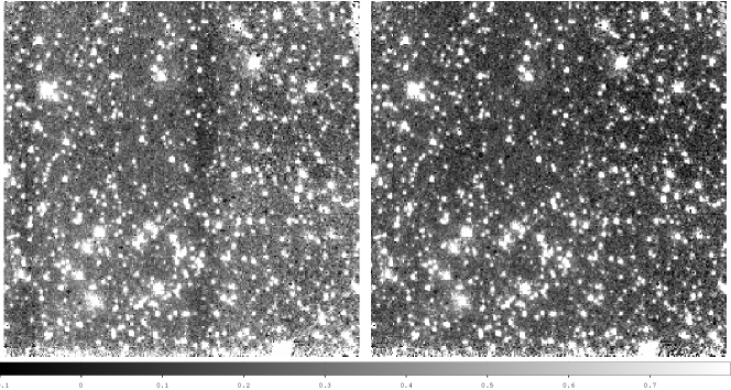
Figure 1: Comparison of the outputs from ‘calnica’ with the application of the STScI provided dark file and the superdark produced with data obtained as part of our program (right panel). The left panel shows two obvious nearly vertical dark lanes. The fuzzy structures at the bottom rows of both images are due to the vignetting problem; these rows are removed from the subsequent data reduction.

First, because the multiple components contributing to the instrumental dark signature can vary with the thermal state of the instrument and telescope on multi-orbit timescales, our dark frame acquisition strategy allowed for reference file acquisition and creation individually for each orbit. The assemblage of dark data themselves, however, along with the NIC1 temperature sensor data for a proxy for the off-scale ${\sl NIC3}$ thermal sensor, indicates that the stability flanking all of our observations at a level of $\leq$ +/- 50 ${\rm mK}$. We therefore choose to produce a single high S/N ‘superdark’ by median combining our dark exposures from all orbits. In order to check the reliability of this ‘superdark’, we examine the differences between output files using this superdark and a dark file produced by only median-averaging the 16 dark exposures in the same orbit. We select a single dithered exposure (na133id1q) for this comparison, since it covers a sky location having low surface brightness and dominated by the instrument background. While the small difference ($<5$%) indicates the similarity of these two dark files, the pixel value distribution of the calibrated image with the ‘superdark’ is much smoother than that from the other dark file, suggesting the higher S/N of the ‘superdark’ file. The superdark significantly reduces the observed ‘Shading’ effect — a noiseless signal gradient in the detector (NICMOS Data Handbook, Thatte et al., 2009); the effect is readily apparent if the dark calibration file provided by the OPUS pipeline is used, which was produced in 2002 (Fig. 1).

Next, utilizing all of the 4068 dithered exposures obtained for the science survey, we construct a new empirical mask file to identify the locations of bad pixels (hot, cold or ‘grot’) in ${\sl NIC3}$. We calculate the intensity median and 68% confidence error ($\sigma$) among the pixels of each dithered exposure and record those pixels with intensities deviating from the median by 1$\sigma$. We consider a pixel to be bad if it is flagged in more than 75% of the exposures. In total, we identify 476 new bad pixels, in addition to 695 in the origin mask file provided by STScI, which used a more conservative threshold. We compare this new mask file with the science exposures and find that these new bad pixels are real. These bad pixels together represent 0.7% of the total number of ${\sl NIC3}$ pixels. The bad pixel mask also includes the following: 1) the bottom 15 rows, which show a steep sensitivity drop due to the vignetting problem (NICMOS Data Handbook, Thatte et al., 2009), 2) a three-pixel-wide zone at the other three boundaries to avoid any potential edge effects and 3) a 10$\times$50-pixel region in the top-right corner, which was contaminated by the residual of the amplifier readout and shows an unusual intensity enhancement, even after we have subtracted the dark file (Fig. 1). All these bad pixels are removed from the individual exposures before further processing.

The flat fields used in the initial pipeline processed data were taken in May 2002, during the SMOV3B operations, shortly after the installation of the cyro-cooler. Since May 2002, flats for ${\sl NIC3}$ F187N and F190N were obtained several times by the STScI. We retrieve ${\sl NIC3}$ F187N and F190N flat field observations taken in September 2007 as part of the Institute’s calibration program. These flat observations are the closest in time to our program observations. We then process these observations for use as the flat field images for our observations. By using the September 2007 calibration data, we are able to correct for a persistent large-scale flat field structure that is correlated over scale-lengths of ten or more pixels, and which lead to localized systematic errors in flat field corrections on the order of $\sim$ 2%.

2.2 DC Offset Corrections

In an individual exposure, obvious differences in background levels exist among the four quadrants. This phenomenon is called the ‘Pedestal’ effect, a well-known NICMOS artifact due to independent DC biases in the quadrants, each of which has its own amplifier for data readout (NICMOS Data Handbook, Thatte et al., 2009). Within a quadrant, however, the bias is constant. This effect must be rectified to correctly map out the surface brightness distribution.

The IRAF routine ‘pedsub’ is commonly used to correct for this effect (before the application of the ‘Drizzle’ package discussed below). The routine consists of three steps: 1) estimating the DC bias level independently for each quadrant; 2) determining the DC bias offsets among different quadrants by matching the surface brightness smoothly across their boundaries; and 3) removing the offsets from the respective quadrants. To do the matching in Step 2, one needs to choose (by trial and error) a method (median, mean, or polynomial fitting). This approach works poorly, however, when the intrinsic surface brightness changes abruptly across the boundary between two adjacent quadrants (e.g., when the change cannot be fitted well by any of the methods).

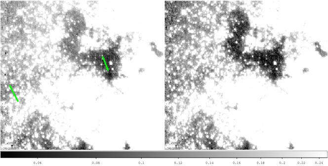
Figure 2: Comparison between the position images that use either the ‘Pedsub’ step 2 (left panel) or our self-calibration method (right panel) in two overlapping regions of quadrants. The green arrows in the left panel point to the places that illustrate flux jumps at the boundaries of the quadrants of individual dithered exposures. This Pedestal effect becomes much more prominent in an image containing net Paschen-$\alpha$ emission.

We have thus developed an effective self-calibration method to determine the DC bias offsets from the overlapping regions among the four dithered exposures taken at each pointing position (diagrammed in Fig. 3). Although individual quadrants in a single exposure have independent sky coverage, they become connected with each other via the square-wave dither pattern. After aligning the four dithered exposures, we identify all overlap regions (see §2.3). There are a total of 48 different overlapping region pairs in each of the four dithered exposures. The mean intensity in an overlapping region can be expressed as $f$=$f_{s}$+$f_{DC}$ where $f_{s}$ is the sky background, and $f_{DC}$ is the DC bias offset. Since $f_{s}$ should be the same in identical quadrants observing the same piece of sky, the measured difference provides a relative measurement of the DC bias offset level. In fact, we can simultaneously determine all the offsets in the 16 quadrants contained within a single pointing position, by conducting a $\chi^{2}$ fit to the differences in the 48 overlapping region pairs (see Appendix). While only 15 of the 16 offsets are independent, we add another constraint that their sum equals zero (i.e., no net bias changes averaged across a position image). Without the trial and error, as would be needed in the replaced Step 2 in ‘pedsub’, our self-calibration method provides an efficient method for removing the ‘Pedestal’ effect (Fig. 2). Upon completion of this step, the relative DC offsets between the quadrants of a single exposure, and between the four dithered images of a single pointing position have been effectively set to a common DC level.

Next, we need to remove the DC offsets between the four pointing positions, within a single orbit and between the 144 different orbits. We adopt the same global fitting method as used for the quadrant offset problem above to estimate the relative DC offset differences among pointing positions within an orbit, and between the 144 different orbits. We first calculate the mean difference between two adjacent pointing positions and the statistical error based on their overlapping region. This fitting methodology therefore leads to 575 linear equations. Again we add the additional requirement that the sum of the corrections in the 576 positions to be zero. The resultant solutions for the 576 offset corrections are added back into the original position images, thereby effectively normalizing all of the images to a single DC offset level.

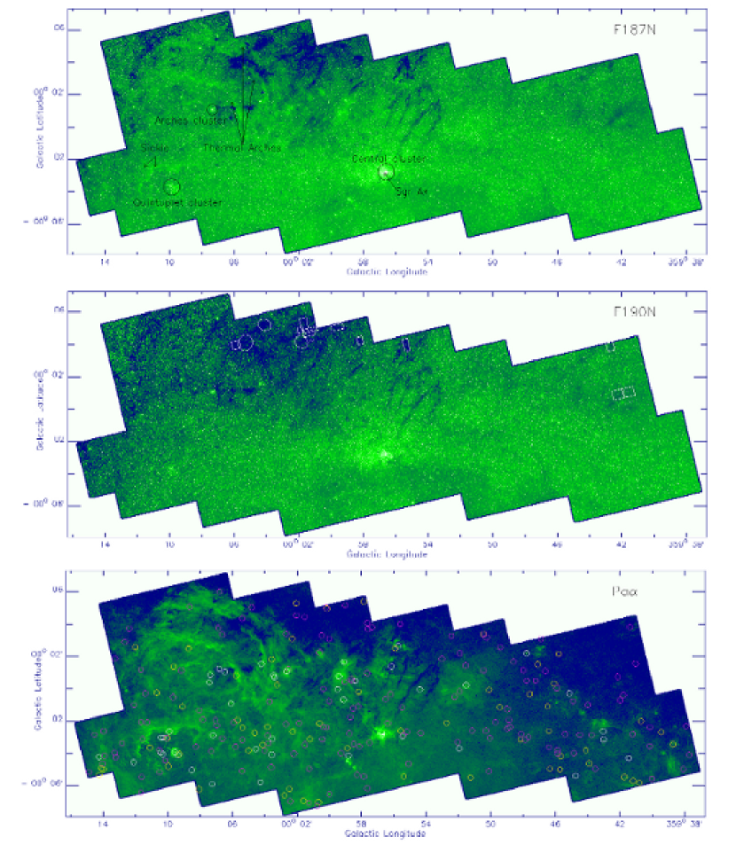
Figure 10: Mosaic images of the F187N, F190N and Paschen-$\alpha$ intensities. In the upper panel, several well-known objects in the GC are marked. White circles and boxes in the middle panel enclose regions used to calculate the absolute background level in the images (see §2.2). The white, yellow and pink circles in the lower panel represent the spectroscopically confirmed, unconfirmed primary and secondary Paschen-$\alpha$ emitting sources, respectively (see §3.5). For clarity, the sources within the cores of the three clusters have not been overlaid.(You can find the full resolution image in www.astro.umass.edu/ dongh/paper/HST-GC-SURVEY/fig10.ps)

In order to calibrate our normalized survey images to the true background count rate, we use a set of very dark regions in the F187N and F190N bands to establish the zero levels (Fig. 10). These regions which are observed to be extended and dark, against the bright near-IR background of the GC, must be caused by the very strong extinction of foreground molecular clouds (i.e. close to the solar neighborhood). We assume there is no detectable astrophysical flux above the instrumental sensitivity over these regions. Therefore, any residual measured counts in these regions are due to the global DC offset level that is a result of the background minimization methodology discussed above. To minimize the effect of the statistical uncertainties in our estimation, we fit the histogram of the intensities obtained in pixels of the dark regions with a Gaussian. The fitted Gaussian central intensity value is adopted as the absolute background and is subtracted from all images.

To convert from the instrumental count rate to physical flux intensities, in the final of the background-subtracted images at 1.87 and 1.90 $\mu$m, we apply the scale factors (PHOTFNU) of 4.32 and 4.05 $\times 10^{-5}$ Jy (ADU $s^{-1}$)^-1, which are obtained from the HST NICMOS Photometric webpage.

2.3 Position image construction

After removing the DC offsets from the entire survey as discussed above, we merge the four individual dithered exposures to form a combined image, which we call the ‘position image’. We do not use the standard IRAF ‘calnicb’ for this task. As mentioned in the HST NICMOS Data Handbook (Thatte et al., 2009), ‘calnicb’ does not allow for pixel subsampling and hence provides no improvement of the image resolution from the use of the dithering. This routine also does not correct for geometric distortion (the pixel size as projected on the sky in the X direction is about 1.005 times larger than that in the Y direction for ${\sl NIC3}$). Instead, we use the IRAF ‘Drizzle’ package to merge the exposures. This package is widely utilized for such a task. Allowing for the dithering resolution enhancement, ‘Drizzle’ uses a variable-pixel linear reconstruction algorithm, which is thought to provide a balance between ‘interlacing’ and ‘shift-and-add’ methods. The behavior of this algorithm is determined by the parameter ‘pixfrac’, which defines the fraction of the input pixel size to be used for the output one. We fix the parameter to be 0.75. With the correction for geometric distortion, an output image is uniformly sampled to 0.101$\arcsec$ square pixels, half of the original pixel size of ${\sl NIC3}$ (i.e. ‘SCALE’=0.5 in ‘Drizzle’). Step-by-step, ‘Drizzle’ first uses ‘crossdriz’ to produce ‘cross-correlation’ images between the different exposures, then ‘shiftfind’ to determine the relative spatial shifts between the exposures, and finally ‘loop_driz’ to merge the exposures into a single position image. The pixel size of the new images below is 0.101$\arcsec$ .

The ‘Drizzle’ package provides additional tools to identify the outliers which are not recognized by ‘calnica’. Toward the same line-of-sight within the four dithered exposures, these tools select out the outlier pixels which cannot be explained by the Poisson uncertainty of the detector’s electrons. These pixels are removed from the further merge process in ‘loop_driz’. However, these tools could potentially identify the core of bright sources in several dithered exposures as cosmic-ray, due to the undersampling problem of the ${\sl NIC3}$ and could make us underestimate the intensity of these sources (see also § 3.5).

2.4 Astrometry correction

Before combining all the position images to form a mosaic map for each filter, we need to correct for different astrometrical uncertainties. We first account for the relative shift between the two filter images of each position, due to the cumulative uncertainties introduced by the small angle maneuvers associated with the relatively large offset dithers. We calculate the shift using 50 or more relatively isolated bright sources, detected in both filters. The largest shift is $\sim$ 0.025$\arcsec$, consistent with the expected HST astrometric accuracy, $\sim$ 0.02$\arcsec$, for observations with at least one guide star locked and within a single orbit (HST Drizzle Handbook). Such a shift, though small, could still significantly affect an effective continuum subtraction (especially in the vicinities of relatively bright sources) required to produce a high-quality Paschen-$\alpha$ image. We thus correct for the shift for each position by regridding the F187N image to the corresponding F190N frame using IRAF ‘geotran’ with interpolation. But we neglect any relative shift between different positions in the same orbit. Such a shift should be similar to that between the filters and thus much less than the image pixel size. We directly merge the four pointing positions to form a mosaic image for each orbit, using the coordinate information in their fits headers.

We need to correct for the relative shifts between orbit images. Each of these images is created by combining the four position images within each orbit with ‘Drizzle’. Because different orbits often used different guide stars, we expect a relatively large astrometric uncertainty, which could be up to about 1$\arcsec$ and must be corrected for before creating a final mosaic map of the entire survey region. According to the ‘Drizzle handbook’, the roll angle deviation of HST is less than 0.003 degrees, i.e. 0.002$\arcsec$ at the edge of the ${\sl NIC3}$. Therefore, we just include the $\alpha$ and $\delta$ shift, but no rotation deviation in our astrometry correction process, for simplicity. We determine the relative shifts among all 144 orbits in a way similar to that used for the instrumental background DC offsets (§2.2). We estimate the relative shifts and their errors (in both $\alpha$ and $\delta$ directions) between two adjacent orbits via the cross-correlation in the overlapping region. A total of 254 pairs of the relative shifts ($\Delta\alpha_{i,j}$ and $\Delta\delta_{i,j}$) are thus obtained. The global fit is then reduced to solve 2$\times$143=286 equations for the required $\alpha$ and $\delta$ corrections to be applied to the 143 orbit images. Fig. 4 compares the distribution of the relative spatial shifts between adjacent orbit images ($\sqrt{\Delta\alpha_{i,j}^{2}+\Delta\delta_{i,j}^{2}}$) before and after the correction. The astrometric accuracy after the correction is sustantially improved; the median and maximum of the shifts are 0.039$\arcsec$ and 0.107$\arcsec$, representing the relative astrometric precision of our survey.

Finally, we calibrate our astrometrically aligned survey image to the absolute astrometry of the Galactic center, by using the precisely measured positions of SiO masers known within the central 1’ around Sgr A* (Reid et al., 2007). These SiO masers, believed to arise from the circumstellar envelopes of giant or supergiant stars, have well-determined positions with uncertainties of only $\sim$ 1 mas (Reid et al., 2007). We adopt the radio positions of the masers determined in March 2006 and account for their proper motions (Table 2 in Reid et al. (2007)). We identify 11 counterparts of our F190N sources (see section 3.1) among the 15 masers; the remaining four (ID 11, 12, 14, 15; Table 1 of Reid at al. 2007) are apparently below our source detection limit and are thus not used. We then correct for the mean $\alpha$ and $\delta$ shifts estimated between the radio and F190N positions of the masers [($\Delta\alpha$, $\Delta$$\delta$)=(0.03$\arcsec$,0.41$\arcsec$)]. After this correction, the median and maximum spatial shifts between the radio sources and their F190N counterparts are 0.03$\arcsec$ and 0.08$\arcsec$, consistent with the residual astrometry uncertainty of our final mosaic maps mentioned above. Therefore, the final median astrometric accuracy of the mosaic is $\sim\sqrt{0.039^{2}+0.03^{2}}=0.049\arcsec$.

3 Data Analysis

With the data cleaned, background-subtracted, and corrected for the astrometry, we conduct data analysis to detect point-like sources, to construct the extinction and Paschen-$\alpha$ maps, and to identify Paschen-$\alpha$-emitting candidates.

3.1 Source Detection

We use IDL program ‘Starfinder’ for the source detection (Diolaiti et al., 2000). This routine, based on point spread function (PSF) fitting, is well-suited to detect and extract the photometry of relatively faint sources in a crowded field, as in the GC. Here we describe the key steps:

3.1.1 PSF construction

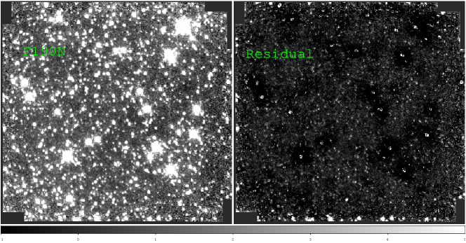
Figure 5: Comparison of the original F190N image (left panel) and the residual image after removing the sources with our own PSF (right panel). We remove the sources near the edge from our catalog of each individual position because of the unreliable photometry. That is why these sources still exist in the residual image

Given the expected stalibity of the HST PSF, and the difficulty of finding truly isolated PSF source stars in the crowded GC, we construct a single PSF for use throughput the entire survey. We select 23 PSF template stars from our images with $m_{K}<$ 7 from the 2MASS catalog which are isolated and have high quality stellar counterparts in our survey. These stars are randomly located in 22 position images (2 stars are located within the same image) and are relatively bright so that any effect due to the presence of adjacent sources and/or small-scale background fluctuation is small. For each star, an image of 128$\times$128 pixels ($\sim$ 12.8$\arcsec$$\times$12.8$\arcsec$) is extracted from the resampled position image. The resultant 23 star images are then normalized and median-averaged (pixel-by-pixel) to form a 2-D PSF. We apply this PSF image to model and subtract the contributions from any obvious adjacent sources in each star image. The PSF image is then formed again. These last two steps are iterated twice to minimize the effect of adjacent sources on the final PSF image. In Fig. 5, we present the original F190N image for one position and its residual image after removing the sources to demonstrate the goodness of our PSF.

3.1.2 Local background noise level

Another key input to the source detection routine is the average noise level ($\bar{\sigma}{{}_{b}}$) of the background in each position image. To remove any large scale diffuse features, we first subtract a median-filtered image (filter size=1.2$\arcsec\sim$ 5 FWHM of the PSF; §3.1.1) from the position image. We then fit the histogram of residual intensity values with a Gaussian to determine the pixel-to-pixel intensity dispersion, which we use as an estimate of $\bar{\sigma}{{}_{b}}$. This fit is not sensitive to the high intensity tail that is due to the presence of relatively bright stars. The median value of the dispersions is 0.017 ADU $s^{-1}$ $pixel^{-1}$, consistent with the estimate from the NICMOS Expsoure Time Calculators (ETC), indicating that they are mostly due to fluctuations in the instrumental background. But positions near Sgr A* show exceptionally large dispersions ($\sim$ 0.03-0.04 ADU $s^{-1}$ $pixel^{-1}$), because of a high concentration of stars, resolved and unresolved.

3.1.3 Source detection process

With the PSF and $\bar{\sigma}_{b}$ as the inputs, we conduct the source detection, which follows the following major steps: 1) Each position image is median-filtered (filter size = 9$\times$FWHM of the PSF) for a local background estimation; 2) A pixel brighter than all 8 immediate surrounding ones and $\gtrsim 6\bar{\sigma}_{b}$ above the local background is identified to be a source pixel candidate; 3) Such pixels are sorted into a descending intensity order; 4) Starting with the highest intensity one, the coefficient of the correlation between the PSF and the surrounding sub-image that encloses the first diffraction ring is calculated; 5) A source is declared if the correlation coefficient is larger than 0.7; 6) This source with its centroid and photometry estimated from the PSF fitting is subtracted from the image before considering the next pixel. When one iteration is completed, all the detected sources are subtracted from the original image and the same steps are repeated again until no new source is detected.

All photometry measurements are performed on the position images prior to construction of the full survey mosaic. For each individual position image, we first detect the sources in the images of F187N and F190N, independently. If two detections from these two filter images are less than 0.1$\arcsec$ apart, we then consider that they are the same source. We also remove all detections that occur only in one filter. With the centroid fixed to the detections of the F190N, we rerun ‘Starfinder’ to obtain the photometry of the remaining sources in both filters.

We remove or flag potentially problematic detections. Those detections with bad pixels within the first diffraction ring are flagged in Table. 2 (‘Data Quality’ = 1). We throw away those detections that are less than 2$\times$FWHM away from an image edge, which, if real, should mostly be detected with better photometry in other overlapping position images. We also identify false detections due to point-like peaks present in the PSF wings of bright sources. For an arbitrary pair of adjacent detections (separation $r<$2$\arcsec$), we estimate the PSF wing intensity of the brighter one at the centroid position of the dim one. If this intensity is greater than the net peak intensity of the dim source, we mark it in Table. 2 (‘Data Quality’= 2).

We merge the detections from all the position images in both filters to form a single master source list. Two sources are considered to be the same, if they are less than 0.25$\arcsec$ apart (FWHM of our PSF) and are from different position images (after the astrometry is corrected; §2.4). The source parameters are adopted from the detection that is farthest away from the position image edges.

3.2 Source detection completeness limit

The source detection completeness varies from one position to another, chiefly because of the variation in the stellar number density. We estimate the average completeness in each position via simulations. We simulate sources in the magnitude range from 13 to 18 with a bin size of 0.5, add them into each position image, and rerun the source detection. Ten separate simulations, each containing 30 sources, are conducted for each magnitude bin. Fig. 6 illustrates the magnitude dependence of the recovered fraction of simulated sources for the two positions with the most extreme stellar number densities: the lowest density position (GC-SURVEY-242) is on the Galactic north side with a foreground dense molecular cloud, while the densest one (GC-SURVEY-316) is near Sgr A*. For this latter position, the fraction decreases quickly as the magnitude increases; the 50% incompleteness limit is about 15.5 mag. This limit increases to 17.5th mag for the lowest density case. For a more typical position in our survey, the 50% incompleteness limit is about 17th magnitude.

3.3 Photometric Uncertainties

It is known that ‘Starfinder’ severely underestimates actual photometric uncertainty (Emiliano Diolaiti, private communication). Therefore, we need to find a better way to accurately formulate and calculate the uncertainties based on our empirical data. The photometric uncertainty should normally consist of at least two parts: 1) the Poisson fluctuation in the intensity ($\propto\sqrt{f}$, where f is the source intensity in units of counts) and 2) the local background noise ($\propto\sigma_{b}$). In the case of ${\sl NIC3}$, we also need to account for the ‘intrapixel’ error, which is due to the response variation over an individual detector pixel from the center to the edge and due to the dead zones between the pixels. This error depends on the degree of the undersampling of the PSF, as is the case for individual ${\sl NIC3}$ exposures. Furthermore, when converting the units ${\rm ADU/s}$ to ${\rm Jy}$, a systematic error ($f_{pe}$) is introduced into the photometry, 0.0168 for F187N and 0.0051 for F190N, involving the use of the calibrated stars. Both of this systematic error and the ‘intrapixel’ error are reduced by a factor of the square root of the number of the dithered exposures used in constructing a position image. Putting all these together, we can express the total model photometric uncertainty $\sigma_{f}$ (in units of ${\rm ADU/s}$) as

$$\sigma_{f}^{2}-A*\sigma_{b}^{2}=\frac{f}{gain*t*N_{exp}}+\frac{(a*f)^{2}+(f_{pe}*f)^{2}}{N_{exp}},$$ (1)

where $f$ (in units of ${\rm ADU/s}$) is the source flux, $t$ (${\rm s}$) is the exposure time for individual dithered exposure, $N_{exp}$ is the total number of exposures, ‘gain’ (6.5 ${\rm electron/ADU}$ for ${\sl NIC3}$) is an instrument parameter, and ‘A’ is the photometry extraction area in units of pixels. The local background noise $\sigma_{b}$ (${\rm ADU/s/pixel}$) can be significantly different from the $\bar{\sigma_{b}}$, the mean background over a position image used in §3.1.2, and can be quantified for each detected source (see below). So only the coefficient $a$ needs to be calibrated for NIC3 .

We conduct this calibration by measuring the flux dispersions in multiple dithered exposures of our detected sources. We select only those sources that are not flagged and are detected in all four dithered exposures of a position. We measure the source flux in each exposure, using the ‘daophot’ package in IRAF (‘Starfinder’ is not suitable for this purpose, because the PSF in a single exposure is severely undersampled). The flux is extracted from an on-source circle (radius=3 pixels or $\sim$ 0.6$\arcsec$, hence $A=3^{2}\pi$) after a local background estimated in an annulus 1$\arcsec$-2$\arcsec$ (4-8 FWHM of the PSF) is subtracted. The median of the standard dispersions within this background region from the four dithered exposures gives $\sigma_{b}$. The mean and standard dispersion of the fluxes ($f$ and $\sigma_{f}$) in the four dithered exposures are then calculated. To conduct a $\chi^{2}$ fit of Eq. 1 to the measurements, we further calculate the average and standard dispersion of $\sigma_{f}^{2}-A*\sigma_{b}^{2}$ (the left side of Eq. 1) in each bin of $20$ sources obtained adaptively from ranking their mean fluxes. The calculated values are presented in Fig. 7. Since $\sigma_{f}$ is the dispersion of the flux measurements among the dithered exposures, $N_{exp}=1$ and $t=48$ s. The best-fit ($\chi^{2}$/dof=4270./2624) then gives $a=0.03$. Fig. 7 compares the empirical measurements and the best-fit model. The dispersion is dominated by the source and background counting uncertainties in the low flux range and by the ‘intrapixel’ error in the high flux one.

With the calibrated $a$ value, we can now convert Eq. 1 for estimating the photometric uncertainties of our sources detected with ‘Starfinder’ (§3.1.3). In this case, the error is for the mean source flux $f$ in a combined position image, instead of the standard dispersion of the detections in individual dithered exposures used in the calibration above. The conversion can be done by setting (1) $N_{exp}$ equal to the actual number of exposures covering each source (typically four), (2) $A$ to $9^{2}$ ${\rm pixels}$, the region (including the first diffraction ring) used to estimate the source flux in ‘Starfinder’ above, and (3) $\sigma_{b}$ to the standard dispersion in a box of 9$\times$9 FWHM in the ‘Starfinder’ residual intensity images obtained after excising all detected sources according to the PSF. The converted Eq. 1 is then used to estimate the photometric uncertainty for each of our detected sources.

A source flux ($f$) may be further expressed in magnitude as

$$m=-2.5{\rm~{}log}(\frac{f}{f_{0}}),$$ (2)

where we adopt the Vega zeropoint ($f_{0}$) as 803.8 Jy (F187N) or 835.6 Jy (F190N), as listed in the NICMOS photometric keywords website.

We also need to have an absolute calibration of our photometry measurements in the F187N and F190N bands. The measurements depend on the goodness of the PSF as well as the calibration of the F187N and F190N transmission curves. We conduct this calibration by comparing our flux measurements with predictions from stellar model spectral energy distribution (SED) fits to 2MASS JHK measurements, which have an excellent photometry accuracy (Skrutskie et al., 2006). We first select out 252 sources with J$<$14.1, H$<$11.6 and K$<$9.8, which insure that these sources are 10% brightest in all three 2MASS bands and show minimal flux confusion from other sources. We construct various SEDs from the ATLAS9 stellar atmosphere model (Castelli et al., 1997), together with the surface temperature and gravity for stars of different types. For each source, we adopt the SED that gives the best $\chi^{2}$ fit to the JHK measurements with the extinction as a fitting parameter (the extinction law of Nishiyama et al. 2009 is assumed). 26 among these 252 sources are chosen because of their low extinction ($A_{K}<0.5$) and without substantial deviation ($<3\sigma$) from the best-fit SES model predictions in F187N. The former criterion is used to reduce the uncertainty in the extinction law that is discuss in § 5, while the latter one removes potential evolved massive stars with significant emission in the 1.87 $\mu$m. The fluxes from the best-fit SED are all consistent with our measurements. The median of the predicted to measured flux ratios for the 26 sources is 1.016$\pm$0.009 (F187N) or 1.049$\pm$0.009 (F190N). This ratio is insensitive to the assumed extinction law ($<$1%, which is used as a measurement of the systematic uncertainty of the F187N to F190N flux ratio later) and is multiplied to the measured F187N or F190N flux, respectively. If we do not modify the absolute photometry here, the flux ratio ($\frac{f_{1.87~{}{\rm\mu m}}}{f_{1.90~{}{\rm\mu m}}}$) would be overestimated by 3% and therefore the extinction derived in § 3.4 would be underestimated by 40%.

3.4 Ratio Map

To construct the net Paschen-$\alpha$ map, we need to subtract the stellar continuum contribution in the F187N band (§3.6). This contribution can be determined by using the observed intensity in the F190N images and the ratio of the F187N and F190N filters. The two primary contributions to the variation in the F187N to F190N ratio are the interstellar extinction and the wavelength differences of the stellar continuum which varies slightly with stellar type. In the GC, the extinction effect dominates, which can be estimated from the F187N to F190N flux ratios of our detected point sources.

Limited by the number statistics of the sources, we construct our ratio map with a pixel size of 4$\arcsec$. For each pixel, we obtain a median F187N to F190N flux ratio ($\overline{r}$) from 101 closest sources as the representative of the F187N to F190N continuum flux ratio of the GC stellar light at that location. The number ‘101’ is considered to be a good balance between reducing the effect of the photometric uncertainty in the median averaging and increasing the angular resolution of our ratio map. As long as the bulk of the 101 sources are low-mass stars located in the GC, the median averaging should not be sensitive to a few outliers (e.g., massive stars or foreground stars). The photometric uncertainty of the averaging ($\sigma_{\overline{r}}$) is $\frac{1}{\sqrt{101}}$ of the standard dispersion estimated from the ranked values (34 on each side of the median). While the median photometric error of individual stars is $\sim 4\%$, the uncertainty after the average should then be $\sim 0.4\%$. We also record the maximum angular distance ($d$) of these sources to the pixel center, which is as small as 4.3$\arcsec$ in the field close to Sgr A*, where the surface density reaches $\sim$ 1.7 sources arcsecond^-2 and has a median of 9.2”, averaged over the whole survey area. This latter value may be considered as the average resolution of the ratio map.

We use the ratio map to construct a high resolution extinction map. Assuming an extinction law: A($\lambda$)=$\lambda^{-\Gamma}$, the differential extinction at each pixel is

$$A_{F187N}-A_{F190N}=((\frac{1.9003}{1.8748})^{\Gamma}-1)\times A_{F190N}=-2.5\times{\rm log}[(\frac{f_{1.87~{}{\rm\mu m}}}{f_{1.90~{}\mu m}})_{o}/(\frac{f_{1.87~{}{\rm\mu m}}}{f_{1.90~{}{\rm\mu m}}})_{m}]$$ (3)

where $(\frac{f_{1.87~{}{\rm\mu m}}}{f_{1.90~{}{\rm\mu m}}})_{o}$ and $(\frac{f_{1.87~{}{\rm\mu m}}}{f_{1.90~{}{\rm\mu m}}})_{m}$ are the observed and intrinsic (model) flux ratios, while (1.9003/1.8748) is the ratio of the effective wavelengths of the two filters. As discussed previously, $(\frac{f_{1.87~{}{\rm\mu m}}}{f_{1.90~{}{\rm\mu m}}})_{m}$= 1.015 for a K0III star and is not very sensitive to the exact stellar types assumed ($<$ 1% for different types of evolved low mass stars). The above equation indicates that there is an anti-correlation between the $\Gamma$ and $A_{F190N}$. To infer $A_{F190N}$ or equivalently $A_{K}$, we assume $\Gamma=2$ (Nishiyama et al., 2009), which seems to be most consistent with the RC magnitude location of stars in the GC (§ 5). If a different extinction law is adoped, then the inferred extinction is changed; e.g., $A_{F190N}$ or $A_{K}$ needs to be scaled by a factor of 1.29/0.91/0.75 or 1.37/0.88/0.69 for $\Gamma$=1.56/2.20/2.64, respectively (Rieke, 1999; Schödel et al., 2010; Gosling et al., 2009). The uncertainty in the averaged photometry ($\sim 0.4\%$) also introduces an uncertainty in this extinction map: $\sim$0.22 mag or $\sim$0.16 mag in the $F190N$ or $K$ band.

We note that the above estimate is problematic in regions with very strong foreground extinction. Such regions can be strongly contaminated, if not dominated, by foreground stars. Therefore, the derived ratio can be a poor representation of stars in the GC. We identify such regions to be those having a source number density ($\frac{101}{\pi d^{2}}$) $<$0.31 arcsecond^-2, which corresponds to $\sim$ 2$\sigma$ below 0.38 arcsecond^-2, the density averaged across the survey field. At each pixel of these regions, we adopt the extinction values from Schultheis et al. (2009) (using the conversion $A_{K}$=0.089$A_{V}$), if it is greater than the one from our map. The extinction map of Schultheis et al. (2009) is based on the Spitzer IRAC photometry of red giants and asymptotic giant branch stars and is sensitive to strong extinction. But the map has a relative low resolution of $\sim~{}2^{\prime}$, which is 12 times larger than the average resolution of our extinction map, and it does not resolve compact dusty clouds.

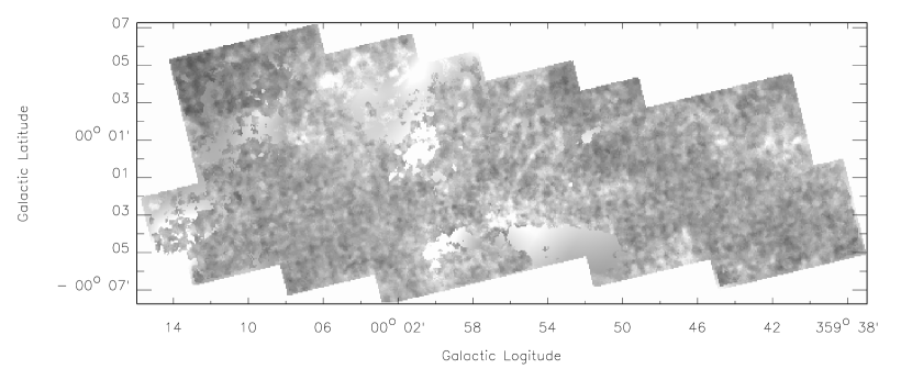
Figure 8: Our adopted extinction map ($A_{F190N}$). White indicate the highest A_F190N values. The minimum, maximum and median values of $A_{F190N}$ are 1.5, 6.1 and 3.0. The spatial resolution is $\sim~{}$9.2$\arcsec$

Our adopted $A_{F190}$ extinction map (or the equivalent flux ratio map) is presented in Fig. 8 and is used for the construction of Paschen-$\alpha$ images. One may infer $A_{K}$, using the conversion, $A_{K}=0.76\times A_{F190N}$, but is advised against a simple conversion to $A_{V}$ because the extinction law is very uncertain between the optical and infrared bands toward the GC (Rieke, 1999; Nishiyama et al., 2009). Because of the closeness of the two filters in our survey, the readers should be aware of the large statistic and potentially systematic uncertainty toward individual lines of sight of the extinction map. The criss-cross ‘textile’ pattern in Fig. 8 appears to be artifacts of relatively large flux uncertainties in the overlapping regions among the pointing positions.

One may be concerned about the presence of stars with Paschen-$\alpha$ absorption lines at 1.87 $\mu$m, which may lead to an overestimation of the extinction. Such stars in a typical region are either too rare (e.g., O and B stars) to affect our median average (used in constructing the extinction map) or too faint (e.g., A-type Main-Sequence stars, which can have significant Paschen-$\alpha$ absorption) to be even detected individually. Only in the core of massive compact clusters may the crowded presence of such stars significantly affect the extinction estimate. We will examine this potential problem in a later paper.

3.5 Paschen-$\alpha$-emitting point sources

We identify a source to be a Paschen-$\alpha$-emitting candidate if its flux ratio $r~{}(=\frac{f_{1.87~{}{\rm\mu m}}}{{f_{1.90~{}{\rm\mu m}}}})$ is significantly above the local background value ($\overline{r}$). We define this excess as

$$r-\overline{r}>N_{s}\sigma_{tot},$$ (4)

where

$$\sigma_{tot}=\sqrt{\sigma_{r}^{2}+\sigma_{\overline{r}}^{2}},$$ (5)

and

$$\sigma_{r}^{2}=\frac{f_{1.87~{}{\rm\mu m}}}{f_{1.90~{}\mu m}}\times\Big{[}\big{(}\frac{\sigma_{f}(1.87~{}{\rm\mu m})}{f_{1.87~{}\mu m}})^{2}+\big{(}\frac{\sigma_{f}(1.90~{}{\rm\mu m})}{f_{1.90~{}\mu m}}\big{)}^{2}\Big{]}.$$ (6)

We choose two values for the significance factor, $N_{s}$, of the excess: 4.5 and 3.5, resulting in the identifications of 197 and 341 potential Paschen-$\alpha$-emitting point sources among all 5.5$\times 10^{5}$ stellar detections having cross-correlation values in both filters larger than 0.8. We use a higher cross-correlation limit here (0.7 in § 3.1.3 ) to remove sources with relative low detection quality. Statistically, the expected number of spurious identifications among all the detected sources is about 2 and 83 for $N_{s}=4.5$ and 3.5, respectively, over the entire survey field. The latter (less conservative) choice $ofN_{s}$ is particularly useful for identifying Paschen-$\alpha$-emitting candidates in small targeted regions (e.g., the known clusters), for which the expected number of spurious sources would be negligible.

We individually examine these initial identifications in the F187N and F190N images to flag potential systematic problems. First, with the choice of $N_{s}$=4.5 (or 3.5), we label 30 (42) of the identified Paschen-$\alpha$-emitting candidates with ‘Problem Index’=1 in Table. 4, since their total fluxes within the central 5$\times$5 pixel in the calibrated F190N images are reduced by 1%, compared with the images produced without ‘cosmic-ray removal’ steps in the ‘Drizzle’ package (see §2.3). Second, each of additional 5 (10) sources has a neighbor within 0.3$\arcsec$ (i.e. $\sim$ 1 FWHM of our PSF) and with a comparable flux (within a factor of 10). The photometric accuracy of these candidates is somewhat problematic. Therefore, they are labeled with ‘Problem Index’=2 in Table. 4. Third, our visual examination removes another 10 sources, the photometry of which are likely affected by the nearby bright sources (‘Problem Index’=3 in Table. 4).

3.6 Paschen-$\alpha$ image

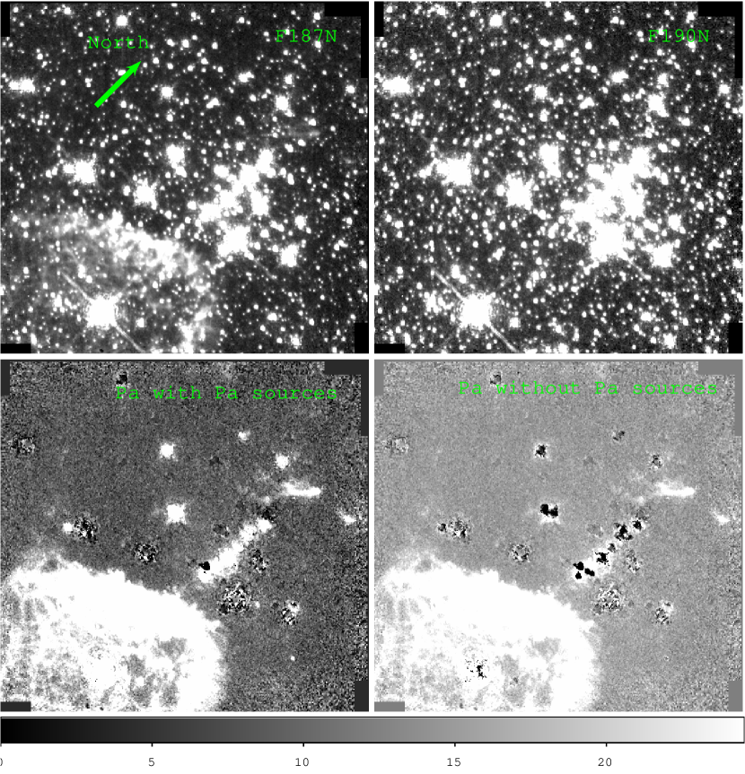
Figure 9: The F187N (upper left) and F190N (upper right) images and differenced images with and without Paschen-$\alpha$ emitting sources (lower left and lower right, see §3.5) of the position ‘GC-SURVEY-72’ (in detector coordinates), which includes the central part of the Quintuplet cluster, the Pistol star and the Pistol Nebula. Diffuse Paschen-$\alpha$ emission from the Pistol Nebula dominates the Paschen-$\alpha$ images.

The final Paschen-$\alpha$ intensity map is created by removing the stellar continuum from the F187N image, using the F190N image and the F187N/F190N point source ratios. The stellar contribution is derived from the F190N intensity image by multiplying a corresponding scale image, which depends on the local intrinsic stellar spectral shape and the line-of-sight extinction determined as described in §3.4. Because of the closeness of the wavelength of the two narrow bands, this dependence is generally weak ($\lesssim 10\%$ for the expected extinction range over the survey area and much smaller for various stellar types). Nevertheless, to map out low surface brightness diffuse Paschen-$\alpha$ emission, we need to account for the dependence, especially for pixels that are affected by relatively bright sources. We construct two kinds of Paschen-$\alpha$ images, with or without the Paschen-$\alpha$ sources ($N_{s}>3$) retained. We denote the latter as denote the diffuse Paschen-$\alpha$ image. We adopt the ‘Spatially Variable Scale’ method used by Scoville et al. (2003) to calculate the scale factor for each individual source that needs to be excised. This method involves many steps, including the allocation of affected pixels to a source and the calculation of its F187N-to-F190N flux ratio. The scale factor for a ‘field’ pixel, which is not significantly affected by sources, is directly inferred from the ratio map constructed in §3.4. This approach adaptively accounts for the spatial extinction variation, which slightly differs from that used in Scoville et al. (2003), where an average flux ratio of detected sources is applied to an entire position image. The product of the constructed scale map and the F190N image is then subtracted from the corresponding F187N image to map out the Paschen-$\alpha$ intensity. Finally, small-scale residuals which deviate from the local median values by more than 50% error (due mainly to photon counting fluctuations around removed sources) are replaced by the interpolation across neighboring pixels in the resultant image, as was done in Scoville et al. (2003). As a close-up demonstration, Fig 9 shows the F187N, F190N and Paschen-$\alpha$ images with and without the Paschen-$\alpha$ emitting sources in the ‘GC-SURVEY-72’ position, which contains the Quintuplet cluster, as well as the Pistol star and its Nebula.

4 Products

Fig. 10 illustrates the products of the above data analysis, including the 1.87 $\mu$m, 1.90 $\mu$m, and Paschen-$\alpha$ mosaic maps constructed for the entire survey field. The diffuse Paschen-$\alpha$ map has been presented in Wang et al. (2010).

Fig. 8 shows our adopted composite extinction map, which represents the first large-scale subarcmin-resolution measurement for much of the survey area. Fig. 11 further presents the $A_{F190N}$ histogram constructed from the map. The median value ($A_{F190N}$) is 3.05, while the peak in Fig. 11 represents $A_{F190N}$=2.92$\pm$0.01, corresponding to $A_{K}=2.22\pm 0.01$ (using the extinction law of Nishiyama et al 2009). If we adopt the extinction law of Rieke (1999), $A_{K}$ increases to 3.03$\pm$0.01, which is consistent with the average extinction ($A_{K}$=3.28$\pm$0.45) derived from stellar observations in 15 different regions within the GC by Cotera et al. (2000). Our estimated extinctions toward the Arches, Quintuplet and Central clusters are also consistent with other independent observations to within 10% (Stolte et al., 2002; Figer et al., 1999a; Scoville et al., 2003), if we adopt the slopes of the extinction laws they used.

In total, we detect 570,532 point-like sources in both the F187N and F190N bands above a threshold of 6$\sigma$. Table 2 presents the parameters for a sample of these sources, while the complete catalog is published online only. Among the sources, 9,662 are flagged because of their proximity to relatively bright sources or because of nearby bad pixels (see §3.1.3 and note to Table 2).

Table 3 presents the 152 sources that are the most reliable Paschen-$\alpha$-emitting candidates, which are identified with $S/N>4.5$ (see § 3.5) and with no flag for potential systematic problems. In addition, we list tentative candidates in Table 4: those with problem flags and S/N $>$ 4.5, and those having 3 $<$ S/N $<$ 4.5.

5 Discussion

The full data set presented in this paper contains a wealth of information on the diffuse ionized gas, the stellar population, and the extinction distribution toward the GC. Here, we focus on the statistical properties of the stellar population; the data alone is typically insufficient for the study of individual stars. Fig. 12 shows the 1.90 $\mu$m magnitude distribution of our detected sources. We further roughly group these sources into the ‘foreground’ ($A_{F190N}<1.8$ inferred from their individual F187N to F190N flux ratios) and ‘background’ ($A_{F190N}$$>4.7$) as well as ‘GC’ components (1.8$<$$A_{F190N}$$<4.7$). The extinction range adopted for the GC component approximately corresponds to 20$<$$A_{V}$$<$50, which is the same as that estimated for the ionized gas within Sgr A West by Scoville et al. (2003), who adopted the extinction law of Rieke (1999). The total source numbers are 1.4$\times 10^{5}$, 1.2$\times 10^{5}$ and 3.1$\times 10^{5}$ in the ‘foreground’, ‘background’, and ‘GC’ components, respectively. This grouping is not meant to be precise, particularly in the consideration of the closeness of the two narrow bands used to infer the extinction and the uncertainty in the photometry. Nevertheless, the components show distinct characteristics in their magnitude distributions, as shown in Fig. 12. The magnitude distributions of the ‘foreground’ and ‘background’ components peak at $\sim~{}17$th mag, which is mostly due to the decreasing detection fraction toward the fainter end. In contrast, the distribution of the ‘GC’ component peaks at 15.80$\pm$0.01, which is far too bright to be due to the source detection limit variation (as demonstrated in Fig. 12b). We fit a gaussian distribution to this peak and obtain a width of 0.67 magnitude, which cannot be explained by the photometric uncertainties of the sources within this magnitude range ($\delta m_{F190N}\sim~{}0.04$). For a prominant old stellar population ($>$2 Gyr) as expected in the GC, the most probable explanation for the peak is the presence of the RC stars, which represent a concentration in the color magnitude diagram (Grocholski & Sarajedini, 2002).

Here we check how this RC explanation is consistent with the peak of the 1.9 $\mu$m magnitude distribution of the GC stars, depending on the specific extinction law assumed (see also § 3.4). The Padova stellar evolutionary tracks show that the RC peak is located at $M_{F190N}=-1.55$ for a 2 Gyr old stellar population with the solar metallicity. We adopted the same distance modulus, 14.52$\pm$0.04, as useed by Schödel et al. (2010). The typical extinction toward the GC in F190N is 2.92$\pm$0.01, as obtained in § 4, assuming the extinction law of Nishiyama et al. (2009). Fig. 13 compares the model and observed magnitude distributions. The RC peak locations of the model (15.89$\pm$0.44) and observations are consistent with each other. In contrast, the RC peak locations predicted from assuming other extinction laws seem to less consistent with the observed one (16.74$\pm$0.51, Rieke 1999; 15.63$\pm$0.41, Schödel et al. 2010; 15.16$\pm$0.35, Gosling et al. 2009). The uncertainties in the peak location of these models are derived from the Eqn. 3 by using 1% systematic error of the F187N to F190N flux ratio (see § 3.3). Therefore, we can see that the Nishiyama’s extinction law best matches our data.

Fig. 14 further compares the GC F190N magnitude contours with stellar evolution tracks, which are obtained from Girardi et al. (2000) for masses in the range of 0.15-7 $M_{\odot}$ and from Bressan et al.(1993) and Fagotto et al.(1994a, 1994b) for 9-120 $M_{\odot}$. In the calculation of the F190N magnitude contours, we have used the line-blanketed stellar atmosphere spectra from ATLAS 9 model (Castelli et al., 1997, and references therein). It is clear that the majority of the GC sources with the limiting magnitudes as discussed in § 3.2 should be mostly evolved low-mass stars, although a significant population can be Main-Sequence (MS) stars with masses $\gtrsim$ 5 (or typically 7) $M_{\odot}$ (i.e. stellar type earlier than B5 or B3).

The ‘background’ and ‘foreground’ components mostly represent the integrated stellar populations along the line of sight in the field. With even larger extinctions and distances than the GC stars, ‘background’ stars should also be mostly evolved (hence intrinsically bright) stars. In comparison, the ‘foreground’ component is likely a mixture of MS and more evolved stars. In particular, the ‘foreground’ distribution shows a knee structure between 15th and 16th mag, which is on the fainter side of the red clump peak. The fainter stars in this structure should mostly be MS and/or subgiants in the foreground Galactic disk.

Our Paschen-$\alpha$ candidate catalog is also contaminated by foreground sources. It is difficult to estimate this contribution based on our data alone. The follow-up spectroscopic observations (Mauerhan et al. 2010c) have shown that two of the 20 confirmed emission line sources appear to be the foreground of the GC. These two sources (stellar type O4-6I and B0I-2I) all have low extinction ($A_{K}\sim~{}1$) and show several He I (2.122$\mu$m, 4S-3P) and H I (2.166$\mu$m, Br$\gamma$) lines; An apparent 1.87$\mu$m intensity excess could then be due to the He I 4F-3D transitions or to the Paschen-$\alpha$ line. Our catalog is further contaminated by non-emission-line foreground stars. For such a star with a smaller line-of-sight extinction than what is assumed for GC stars, the Paschen-$\alpha$ emission excess can be slightly overestimated. In the extreme case of no extinction, $r\sim$1.015, instead of 0.942 for $A_{Ks}\sim~{}2.22$ (Eq. 3). This small overestimation can lead to additional spurious identifications: about 2 and 83 for $N_{s}=4.5$ and 3.5, accounting for the photometric uncertainties of the sources with $r>1$, i.e. $A_{Ks}<0.44$.

To further investigate the line-of-sight locations of our Paschen-$\alpha$ emission sources, we also use 2MASS and SIRIUS catalogs (Skrutskie et al., 2006; Nishiyama et al., 2006) to identify foreground stars which are assumed to have $m_{H}-m_{K}<1$ or $A_{Ks}<1.5$. We first search for the counterparts of our Paschen-$\alpha$ emitting sources from the SIRIUS catalog with both $m_{H}$ and $m_{K}$ measurements. The 2MASS catalog is used as a supplementary. The stars within the three large clusters do not have reliable photometry in the 2MASS and SIRIUS catalogs due to low angular resolutions of these surveys; however, the clusters have been studied in depth elsewhere (e.g. Figer et al., 1999a, 2002; Paumard et al., 2006). In the field regions, we find that 2 and 8 Paschen-$\alpha$ candidates are likely foreground stars (H-K $<$ 1) based on the 2MASS and SIRIUS catalogs, respectively. The two 2MASS sources have been studied in Mauerhan et al. (2010c), as discussed above, and are in fact emission line stars. Therefore, although the eight stars with counterparts in the SIRIUS catalog are likely to be in the foreground of the GC, we can not exclude the possibility that they are still evolved massive stars in the Galactic disk. Further spectroscopic observations are needed to identify their origin.

Our survey identifies almost all of the GC massive stars with strong line emission found in previous studies. We include in Table 3 spectroscopically identified counterparts of our Paschen-$\alpha$ emitting sources, both in the three clusters and in the field regions. In Table 5, we compare our detections with the stars that have been identified spectroscopically in individual clusters or nearby. We assume that massive stars within 3$r_{c}$ (see Table. 5) are cluster members. Our Paschen-$\alpha$ detections (Table 5) recover all 14 sources having the largest equivalent widths of Pachen-$\alpha$ line in Figer et al. (2002), either WNL (WN7-9) or OIf⁺ (Martins et al., 2008). The other massive stars, which are still on or just leaving the MS, tend to show featureless spectra or even absorption lines and are not detected as Paschen-$\alpha$ emitting sources. In the Quintuplet, we missed six of 19 WR stars identified in Liermann et al. (2009), five of which are the Quintuplet-proper members (Figer et al., 1999a), which all lack spectroscopic features in the K band. The sixth star has a similar spectrum. For the two LBV stars appearing in previous literatures (such as, Figer et al., 1999a), we found the Pistol star, but not qF362 (see Mauerhan et al., 2010b, for more discussion on this unusual star).

In the Sgr A West region, source confusion and a significant unresolved background stellar component severely limited our detection of Paschen-$\alpha$ emitting sources. Only 17 of known 31 WR and OIf⁺ stars in the Central Cluster are detected in our survey with $N_{s}>3.5$. Because the IRS 13 E complex is not well resolved in our survey, the WR stars, IRS 13 E4 and IRS 13E2 (E48 and E51 in Paumard et al., 2006) are detected as one source in our catalog. The other 12 massive stars in Paumard et al. (2006) do not pass our detection threshold, at least partly because of the high background. These stars are listed in Table 6.

Among the 13 young massive stars which do not belong to any of the three clusters  (see Mauerhan et al., 2007, and references therein), only one source is not detected as a Paschen-$\alpha$ candidate. This source is only 1.6$\sigma_{tot}$ above the local strong extended Paschen-$\alpha$ emission. The line emission in ground-based spectroscopic observations of the source may be significantly contaminated by the nebula emission, as proposed by Cotera et al. (1999) .

6 Summary

In this paper, we have detailed the data cleaning, calibration, and analysis procedures for our large-scale HST/NICMOS survey of the GC. The key steps in these procedures, implemented specifically for this survey, include: (1) the removal of the telescope and instrument effects, particular the DC offsets within the four quadrants of individual exposures and among different position images; (2) the correction for the relative and absolute astrometry of the data; and (3) the quantification of the photometric uncertainties for sources detected with ‘Starfinder’. Our main products and preliminary interpretations are as follows:

• We have constructed the background-subtracted, astrometry-corrected mosaics of the net Paschen-$\alpha$ intensity as well as the F187N and F190N filter images for the central $\sim~{}100\times 40$ ${\rm pc}$² of our Galaxy, providing high resolution ($\sim$0.2$\arcsec$), high fidelity data with an average sensitivity of $\sim$ 90 $\mu$Jy ${\rm arcsecond^{-2}}$ for F187N and F190N and $\sim$ 130 $\mu$Jy ${\rm arcsecond^{-2}}$ for Paschen-$\alpha$.

• We have built a catalog of $\sim~{}$0.6 million point-like sources detected in the both F187N and F190N filters. These sources contribute up to 85% of the total intensity observed in the F190 band. The 50% detection limit varies from 15.5th magnitude near Sgr A* to 17.5th magnitude in regions of lowest stellar density. The sources should represent predominantly evolved low-mass stars, with a much smaller component consisting of MS or evolved massive stars ($\gtrsim 7M_{\odot}$). A fraction of 54% of the GC sources in the extinction range $A_{F190N}=1.8-4.7$ tend to be substantially brighter (intrinsically) than both foreground and background stars with lower or higher extinction. This trend is most likely caused by the presence of a prominent RC clump (at about 15.8th mag). A steep extinction curve toward the GC (Nishiyama et al., 2009) is needed to simultaneously explain the magnitudes and colors of these RCs.

• We have obtainted a median F187N/F190N flux ratio map, adaptively and statistically constructed from detected source fluxes to trace the foreground extinction of the GC at a spatial resoluition of 10$\arcsec$. This map allows for a more reliable estimation of the F187N band stellar continuum and hence the net Paschen$-\alpha$ emission from the GC. This also provides one of the highest resolution extinction maps of the survey region to date, although the closeness of the two filters may result in large systematic uncertainties in the extinction toward individual lines of sight ($\sim$0.2 mag in K band).

• We have presented a primary catalog of 152 Paschen-$\alpha$ emitting candidates, plus a secondary list of 189 more tentative identifications. These sources mostly represent evolved very massive stars with strong optically-thin stellar winds, as partly confirmed by existing and follow-up spectroscopic observations. In particular, the candidates detected first in our uniform survey are mostly located outside the three known clusters and represent the large-scale low-intensity star formation processes in the exreme environment of the GC. These detections represent a significant increase in the number, and an important diversification in the location, of known young massive stars within the Galactic center.

The data products of the survey, the catalogs and images described in the present paper, will also be released to the public via the Legacy Archive of the Space Telescope Science Institute.

Appendix A Global Parameter Optimization Based on Fitting to Multiple overlapping Regions

In the main text, we have mentioned the use of global fitting to multiple overlapping regions to optimize parameter determinations. Such parameters could be spatial offsets (§2.4) or relative background corrections (§2.2) between adjacent images, constructed for the quadrants, positions or orbits (we call them simply as ‘parts’ below for simplicity). We label the parameters as $\delta\overrightarrow{X}_{i}$, ”i” is the ID for different parts). In each case (the spatial offset or the background correction), we minimize a specific defined global $\chi^{2}$ to the optimal parameters for all parts.

We first define the global $\chi^{2}$. For two arbitrary adjacent parts, their best parameter differences and errors ($\overrightarrow{X}_{ij}$ and $\sigma_{ij}$, $\overrightarrow{X}_{ij}$=-$\overrightarrow{X}_{ji}$, $\sigma_{ij}$=$\sigma_{ji}$) could be calculated from the cross-correlation method (for the spatial offset) or the median difference (for the background correction) through the pixel values in the overlapping region. If two parts are not adjacent, we set $\overrightarrow{X}_{ij}$=0 and $\sigma_{ij}$=$\infty$. Therefore, the formula for $\chi^{2}$ can be expressed as

$$\chi^{2}=\sum_{i,j}\frac{(\delta\overrightarrow{X}_{i}-\delta\overrightarrow{X}_{j}+\overrightarrow{X}_{ij})^{2}}{\sigma_{ij}^{2}}$$ (A1)

Then, in order to get a global minimum for $\chi^{2}$, we can create an equation array.

$$\frac{\partial\chi^{2}}{\partial\delta\overrightarrow{X}_{i}}=\sum_{j}\frac{4\times(\delta\overrightarrow{X}_{i}-\delta\overrightarrow{X}_{j}+\overrightarrow{X}_{ij})}{\sigma_{ij}^{2}}=0\\$$ (A2)

i.e.

$$\left[\begin{array}[]{ccccc}\displaystyle\sum_{j}\frac{1}{\sigma_{1j}^{2}}&-\displaystyle\frac{1}{\sigma_{12}^{2}}&...&...&-\displaystyle\frac{1}{\sigma_{1N}^{2}}\\ -\displaystyle\frac{1}{\sigma_{21}^{2}}&\displaystyle\sum_{j}\frac{1}{\sigma_{2j}^{2}}&...&...&-\displaystyle\frac{1}{\sigma_{2N}^{2}}\\ ...&...&...&...&...\\ ...&...&...&...&...\\ -\displaystyle\frac{1}{\sigma_{N1}^{2}}&-\displaystyle\frac{1}{\sigma_{N2}^{2}}&...&...&\displaystyle\sum_{j}\frac{1}{\sigma_{Nj}^{2}}\\ \end{array}\right]\times\left[\begin{array}[]{c}\delta\overrightarrow{X}_{1}\\ \delta\overrightarrow{X}_{2}\\ ...\\ ...\\ \delta\overrightarrow{X}_{N}\\ \end{array}\right]=\left[\begin{array}[]{c}-\displaystyle\sum_{j}\frac{\overrightarrow{X}_{1j}^{2}}{\sigma_{1j}^{2}}\\ -\displaystyle\sum_{j}\frac{\overrightarrow{X}_{2j}^{2}}{\sigma_{2j}^{2}}\\ ...\\ ...\\ -\displaystyle\sum_{j}\frac{\overrightarrow{X}_{Nj}^{2}}{\sigma_{Nj}^{2}}\\ \end{array}\right]~{}~{}~{}~{}~{}~{}~{}~{}~{}~{}~{}~{}~{}~{}~{}~{}~{}~{}~{}~{}(4)$$

$N$ is the total number of parameters (288 in the astrometry correction, see §2.4, 16 and 576 in the background correction among quadrants and positions, see §2.2). Since either in correcting the background difference in different quadrants, positions (see §2.2) or relative astrometry (see §2.4), we always calculate the relative difference among the parts. Therefore, the equations for the parameters of one part (one equation in background difference calculation and two equation in astrometry correction for $\Delta\alpha$ and $\Delta\delta$ of one orbit) in the equation array should be extra. In order to get an uniform solution, we set $\Delta\alpha_{1}$=0 and $\Delta\delta_{1}$=0 when calculating the relative astrometry (see §2.4) and in the background difference calculation between quadrants and positions (see §2.2), we add one more constrain that the sum of the total background correction for all the parts should be 0. Then through solving the 2$\times(N-1)$ (astrometry correction, the spatial shift of orbit 1 was fixed) or N (the background difference) equations, we can obtain the parameters for the N parts.

Table 1: Survey Parameters

Parameters	Value
Instrument	NICMOS NIC3
Total # of Orbits	144
Sky Coverage (arcmin2)	416
# of Positions per Orbit	4
# of Dither Exposures per Position	4
Field of View of Each Position	$52^{\prime}\times 52^{\prime}$
Filters	F187N/F190N
	(1.87$\mu$m, on-line)/(1.90$\mu$m, off-line)
Effective wavelength	1.8748$\mu$m/1.9003$\mu$m
PHOTFNU	43.2/40.4 $\mu$Jy sec $DN^{-1}$
$F_{nu}(Vega)$	803.8/835.6 Jy
Exposure per Filter/Position (s)	192
Readout Mode	MULTIACCUM

Table 2: HST/NICMOS GC Survey Gatalog

	R.A.	Decl.	Uncertainty				$f_{1.87~{}\mu m}$	$f_{1.90~{}\mu m}$	$\sigma_{f_{1.87~{}\mu m}}$	$\sigma_{f_{1.90~{}\mu m}}$				Data
Source ID	(J2000.0)	(J2000.0)	(R.A.)	(Decl.)	l	b	($Jy$)	($Jy$)	($Jy$)	($Jy$)	$m_{F187N}$	$m_{F190N}$	$N_{exp}$	Quality
(1)	(2)	(3)	(4)	(5)	(6)	(7)	(8)	(9)	(10)	(11)	(12)	(13)
1	266.27877	-29.14364	0.02	0.03	359.76538	-0.01395	5.36	5.35	0.09	0.08	5.4	5.5	4	0
2	266.42287	-28.86000	0.05	0.04	0.07313	0.02640	4.09	4.16	0.07	0.07	5.7	5.8	4	0
3	266.28008	-29.13699	0.02	0.03	359.77165	-0.01146	3.41	3.41	0.06	0.05	5.9	6.0	4	0
4	266.46723	-28.78837	0.02	0.01	0.15452	0.03053	2.90	3.38	0.07	0.08	6.1	6.0	2	0
5	266.51105	-28.99267	0.05	0.01	0.00003	-0.10856	3.27	3.23	0.06	0.05	6.0	6.0	4	0
6	266.26167	-29.11459	0.04	0.02	359.78236	0.01396	2.74	2.87	0.05	0.05	6.2	6.2	4	0
7	266.59299	-28.74451	0.02	0.01	0.24932	-0.04081	2.82	2.85	0.05	0.04	6.1	6.2	4	0
8	266.44895	-29.05837	0.04	0.02	359.91567	-0.09639	2.73	2.78	0.05	0.04	6.2	6.2	4	0
9	266.24587	-29.27417	0.02	0.04	359.63905	-0.05760	2.22	2.31	0.06	0.05	6.4	6.4	2	0
10	266.47656	-28.94451	0.03	0.03	0.02546	-0.05773	2.38	2.29	0.04	0.04	6.3	6.4	4	0
11	266.49101	-28.98780	0.02	0.02	359.99507	-0.09106	1.86	2.11	0.03	0.03	6.6	6.5	4	0
12	266.38384	-28.78755	0.01	0.04	0.11715	0.09334	1.83	1.86	0.03	0.03	6.6	6.6	4	0
13	266.40656	-28.77856	0.02	0.02	0.13519	0.08103	1.59	1.64	0.03	0.03	6.8	6.8	4	0
14	266.48984	-28.74051	0.01	0.04	0.20570	0.03851	1.42	1.41	0.03	0.02	6.9	6.9	4	0
15	266.38173	-29.01626	0.01	0.02	359.92100	-0.02428	1.38	1.40	0.03	0.03	6.9	6.9	2	0
16	266.26673	-29.18231	0.02	0.03	359.72691	-0.02517	1.26	1.40	0.02	0.02	7.0	6.9	4	0
17	266.51293	-28.81531	0.03	0.03	0.15235	-0.01769	1.27	1.30	0.02	0.02	7.0	7.0	4	0
18	266.24782	-29.09057	0.03	0.02	359.79653	0.03682	1.41	1.10	0.02	0.02	6.9	7.2	4	0
19	266.24378	-29.25220	0.01	0.02	359.65684	-0.04457	1.05	1.06	0.02	0.02	7.2	7.2	3	0
20	266.40381	-29.06478	0.03	0.03	359.88964	-0.06605	1.02	1.05	0.02	0.02	7.2	7.3	4	0
…	…	…	…	…	…	…	…	…	…	…	…	…	…	…

Note. — The full source list is published online in the future. A portion is shown here. Units of R.A. and Decl. are decimal degrees, while units of uncertainty is arcsecond. Columns 6 and 7 are in Galactic longitude and latitude in decimal degrees. The sources with the ‘Data Quality’=1 have nearby bad pixels, while the sources with the ‘Data quality’=2 are significantly contaminated by wings of bright sources (see § 3.1.3)

Table 3: Primary Paschen-$\alpha$ emitting candidates

Source	R.A.	Decl.
ID	(J2000.0)	(J2000.0)	H	K	$m_{F190N}$	r	r-$\bar{r}$	$N_{s}$	Counterpart	Type	Location
(1)	(2)	(3)	(4)	(5)	(6)	(7)	(8)	(9)	(10)	(11)	(12)
1	266.62478	-28.78001	12.8	12.6	12.6	1.1	0.15	5.6			F
2	266.59921	-28.80299	13.3	11.4	12.1	2.6	1.64	26.7	Mau10c_17	WN5b	F
3	266.51501	-28.78606	14.1	12.3	13.0	1.1	0.13	4.9			F
4	266.55606	-28.81641	11.5	9.8	10.5	1.2	0.31	10.3	FQ_381	OBI	Q
5	266.55408	-28.82014	14.1	12.2	13.8	1.1	0.17	5.9			Q
6	266.56301	-28.82693	10.5	10.4	9.6	1.5	0.53	15.1	Lie_71,FQ_241	WN9	Q
7	266.56643	-28.82714	10.6a	8.9a	10.2	1.5	0.55	15.4	Lie_67,FQ_240	WN9	Q
8	266.56293	-28.82480	11.2	9.8	10.2	1.2	0.23	8.1	Lie_110,FQ_270S	O6-8 I f (Of/WN?)	Q
9	266.56312	-28.82568	11.1	10.6	10.3	1.1	0.17	6.2	Lie_96,Mau10a_19	O6-8 I f e	Q
10	266.56304	-28.82631	11.6	9.9	10.6	1.1	0.18	6.7	Lie_77,FQ_278	O6-8 I f eq	Q
11	266.56896	-28.82547	11.7	10.2	10.9	1.5	0.52	14.9	Lie_99,FQ_256	WN9	Q
12	266.56323	-28.82821	13.2	11.3	12.2	2.7	1.74	26.8	Lie_34	WC8	Q
13	266.56316	-28.82761			12.2	2.3	1.33	23.8	Lie_47	WC8	Q
14	266.58167	-28.83606			15.2	1.2	0.30	4.8			F
15	266.51338	-28.81622	13.2	11.7	12.4	1.1	0.17	6.4			F
16	266.47853	-28.78699	14.6	13.1	13.6	1.1	0.20	6.8			F
17	266.46028	-28.82543	12.5	10.6	11.3	2.0	1.05	22.1	FA_5,Blu01_22	WN8-9h	F
18	266.45712	-28.82372	13.0	10.8	11.7	1.7	0.79	19.3	FA_2,Blu01_34,Mau1	WN8-9h	A
19	266.45255	-28.82840	13.6	11.1	12.1	1.9	0.97	21.4	Mau10c_11	WN8-9h	F
20	266.45865	-28.82393	12.8	11.0	11.7	1.2	0.29	9.7	FA_10,Blu01_30	O4-6If	A
21	266.45895	-28.82411	13.5	11.6	12.5	1.2	0.26	8.5	FA_17,Blu01_29		A
22	266.47249	-28.82693	12.5	11.0	11.6	1.3	0.31	10.5	Mau10c_12	WN8-9h	F
23	266.54169	-28.92566	12.3	10.8	11.4	1.3	0.33	10.8	Mau10c_15	WN8-9h	F
24	266.50251	-28.90761	15.2	13.6	14.9	1.2	0.25	5.7			F
25	266.49295	-28.87223			14.4	1.2	0.30	8.5			F
26	266.49541	-28.89392	15.5	13.6	15.7	1.4	0.42	4.6			F
27	266.48141	-28.90196	16.2	15.3	15.3	1.4	0.45	7.5			F
28	266.49067	-28.91267	13.4	11.4	12.2	1.9	1.00	21.5	Ho2	WC8-9	F
29	266.53998	-28.95375	16.5	14.4	14.9	1.1	0.17	4.9			F
30	266.53377	-28.97338	12.6	10.5	11.0	1.1	0.18	6.6			F
31	266.52612	-28.98747	13.6	11.7	12.3	1.1	0.12	4.8			F
32	266.37803	-28.87674			17.1	1.6	0.66	5.0			F
33	266.33953	-28.86082			14.2	1.2	0.26	8.1			F
34	266.46061	-28.95726	12.9	11.3	12.0	2.6	1.67	26.9	Mau10c_19	WC9	F
35	266.36926	-28.93473	11.5	9.7	10.6	1.4	0.46	10.8	Cot_4,Mau10a_7	Of	F
36	266.38126	-28.95466	12.7	11.4	11.8	1.1	0.17	6.4	Mau10c_6	O4-6I	F
37	266.44762	-29.04884			15.1	1.2	0.22	4.6			F
38	266.40831	-29.02624	9.6a	8.9a	9.1	1.1	0.13	5.2	Mau10c_7	O4-6I	F
39	266.34458	-28.97893	15.2	12.2	13.4	2.3	1.41	24.8	Mau10a_6	WN5-6b	F
40	266.35029	-29.01633	10.3a	8.8a	9.7	1.2	0.21	7.5	Mau10c_5	B0I-B2I	F
41	266.40788	-29.10817	13.1	11.5	12.1	1.1	0.15	5.9			F
42	266.38541	-29.08277	14.6	12.0	13.0	1.8	0.88	20.1	Mau10c_8	WC9	F
43	266.30814	-29.07728	15.2	13.6	15.6	1.3	0.37	5.7			F
44	266.25555	-29.04208	14.8	11.9	13.1	1.1	0.18	6.6			F
45	266.25250	-29.10650	16.6	14.8	15.8	1.2	0.26	5.2			F
46	266.28706	-29.11563	14.9	13.3	13.9	1.3	0.38	11.1			F
47	266.31271	-29.15230			14.9	1.1	0.17	4.7			F
48	266.34449	-29.18235			15.7	1.3	0.34	6.0			F
49	266.34120	-29.19988	14.7	12.7	13.4	1.9	0.94	20.5	Mau10c_3	WC9	F
50	266.26206	-29.14994			10.6	1.1	0.15	5.8	Mau10a_1	O9I-B0I	F
51	266.26160	-29.13144	16.1	14.5	14.6	1.1	0.18	5.7			F
52	266.22865	-29.11919	16.6	14.8	15.1	1.1	0.17	5.0			F
53	266.27944	-29.20018	13.5	11.1	12.1	1.3	0.34	11.1	Mau10c_2	WC9?d	F
54	266.24580	-29.22798	15.9	13.8	15.0	1.9	0.95	17.2			F
55	266.24935	-29.26869	12.6a	11.9a	14.6	1.1	0.17	5.1			F
56	266.61499	-28.76995	11.3	9.5	10.2	1.3	0.35	11.3	Mau10c_18	OI	F
57	266.62457	-28.77776	14.7	12.6	13.6	1.3	0.38	11.6			F
58	266.63270	-28.77975	12.6	11.6	11.9	1.2	0.34	5.8			F
59	266.57304	-28.82467	11.8a	10.2a	11.0	1.4	0.46	9.6	FQ_274	WN9	Q
60	266.57294	-28.82181	13.4	11.4	12.2	2.2	1.27	24.1	FQ_309	WC8	Q
61	266.48245	-28.74278	15.0	13.3	14.0	1.3	0.35	10.5			F
62	266.55855	-28.82124	12.3	10.5	11.3	2.2	1.24	24.0	Lie_158,FQ_320	WN9	Q
63	266.55437	-28.82364	12.9	10.5	11.5	1.4	0.49	14.4	Ho3	WC8-9	Q
64	266.54641	-28.81830	13.4	11.6	12.3	2.6	1.61	26.5	FQ_353E	WN6	F
65	266.55773	-28.81403	12.7	10.9	11.7	1.1	0.21	7.6	FQ_406		Q
66	266.56483	-28.83833	13.2	11.2	12.2	2.0	1.01	15.3	FQ_76	WC9	Q
67	266.56301	-28.83910			15.6	1.4	0.41	4.6			Q
68	266.56352	-28.83428	8.9a	7.3a	7.3	1.2	0.25	7.6	FQ_134	LBV	Q
69	266.56452	-28.82226	10.8	9.2	9.9	1.1	0.12	4.5	Lie_146,FQ_307	O6-8 I f?	Q
70	266.56973	-28.83090	11.9	10.2	11.0	1.1	0.18	6.4	Lie_1	O3-8 I fe	Q
71	266.55895	-28.82645	12.9	10.3	11.5	1.4	0.45	13.3	Lie_76	WC9d	Q
72	266.56676	-28.82268	12.1	10.5	11.3	1.1	0.14	5.1	Lie_143,FQ_301	O7-B0 I	Q
73	266.56173	-28.83344	13.2	10.5	11.9	1.2	0.22	5.3	FQ_151	WC8	Q
74	266.55722	-28.82803			15.2	1.4	0.46	7.7			Q
75	266.57118	-28.85862	12.1	10.5	11.3	1.3	0.36	11.2	M07_2,Mau10a_22	O6If+	F
76	266.58645	-28.87528	13.7	12.6	13.1	1.1	0.14	4.6			F
77	266.57310	-28.88431	12.1	10.5	11.1	1.5	0.51	14.6	Mau10c_16	WN8-9h	F
78	266.45091	-28.79055	14.6	12.7	13.6	1.1	0.15	5.6			F
79	266.46449	-28.82372	13.2	11.2	11.8	1.5	0.61	11.8	Blu01_1	WN7	F
80	266.46014	-28.82276	11.6	9.9	10.6	2.0	1.09	22.3	FA_6,Blu01_23,Mau1	WN8-9h	A
81	266.46075	-28.82145	11.7	10.1	10.8	2.1	1.21	20.3	FA_4,Blu01_17	WN7-8h	A
82	266.46182	-28.82389	12.0	10.1	10.9	2.1	1.14	22.9	FA_3,Blu01_3	WN8-9h	A
83	266.46035	-28.82199	13.6	12.0	10.7	1.8	0.82	18.8	FA_7,Blu01_21,Mau1	WN8-9h	A
84	266.46001	-28.82246	12.0	10.1	11.1	2.0	1.04	21.6	FA_8,Blu01_24	WN8-9h	A
85	266.45925	-28.82274	12.0	10.1	11.0	1.7	0.79	18.9	FA_1,Blu01_28	WN8-9h	A
86	266.45948	-28.81983	12.2	10.5	11.0	1.5	0.56	11.2	FA_9,Blu01_26,Mau1	WN8-9h	A
87	266.45954	-28.82136	10.0a	9.6a	11.4	1.8	0.86	19.5	FA_12,Blu01_25	WN7-8h	A
88	266.46121	-28.82284	12.4	10.8	11.5	1.6	0.69	17.3	FA_14,Blu01_12	WN8-9h	A
89	266.46151	-28.82118	12.2	10.8	11.4	1.2	0.28	6.6	FA_15,Blu01_8	O4-6If	A
90	266.46057	-28.82231	12.5	10.9	11.7	1.4	0.50	13.3	FA_16,Blu01_19	WN8-9h	A
91	266.48072	-28.85726	12.5	11.0	11.5	2.5	1.61	18.8	M07_1,Mau10a_16	WN5-6b	F
92	266.52345	-28.85881	9.2a	7.5a	7.4	1.3	0.38	11.9	Mau10b	LBV	F
93	266.51671	-28.89814			15.6	1.2	0.30	5.5			F
94	266.51080	-28.90388	13.5	11.6	12.5	2.4	1.42	21.8	Mau10c_14	WC9	F
95	266.49765	-28.88075	12.1	10.5	11.2	1.1	0.12	4.8			F
96	266.45238	-28.83491	13.3	11.0	11.8	2.0	1.10	22.8	Cot_1	Ofpe/WN9	F
97	266.44891	-28.84692	12.2a	10.7a	11.5	1.2	0.25	7.6			F
98	266.42197	-28.86325	11.6	9.9	10.6	1.2	0.27	6.6	Mau10c_9	O4-6If+	F
99	266.41118	-28.86958	16.4	13.9	15.1	1.9	0.95	17.4			F
100	266.42634	-28.87976	11.7	10.1	10.9	1.3	0.37	8.2	Mau10c_10	O4-6If+	F
101	266.42704	-28.88140	13.2	11.2	12.1	1.9	0.98	21.0	Ho1	WC8-9	F
102	266.43349	-28.88800	13.3	12.4	12.8	1.2	0.25	8.8			F
103	266.50689	-28.92091	10.7	9.1	9.7	1.2	0.28	9.7	Mau10c_13	OI	F
104	266.53042	-28.95485			16.3	1.5	0.52	4.5			F
105	266.47070	-28.92692	14.9	13.4	14.0	1.1	0.19	6.2			F
106	266.46776	-28.94615	16.1	14.5	14.7	1.3	0.32	8.1			F
107	266.41391	-28.88919	11.8	10.2	10.9	1.4	0.43	11.4	Cot_5	B[e]	F
108	266.44602	-28.94612	15.5	14.0	14.7	1.2	0.27	6.4			F
109	266.46088	-28.98877	12.5	10.9	11.6	1.9	1.01	19.2	Cot_2,Mau10a_15	WN7	F
110	266.45393	-28.98382	15.7	14.3	15.0	1.1	0.20	4.7			F
111	266.40061	-28.94403	12.3	10.4	11.1	1.8	0.85	20.0	Mik06_01,Mau10a_9	WN8-9h	F
112	266.40753	-28.95450	13.1	10.7	12.0	1.4	0.49	13.8	Cot_6	B[e]	F
113	266.39038	-28.96381	14.2	12.2	12.9	1.1	0.19	6.9			F
114	266.38658	-28.93794	12.1	10.7	11.3	1.2	0.21	7.1	Mau10a_8	O4-6I	F
115	266.32590	-28.89079	13.8	11.9	12.9	1.1	0.16	5.1			F
116	266.29639	-28.91955	13.0	12.8	12.8	1.1	0.16	6.0			F
117	266.41477	-29.00973	12.7	10.3	11.6	2.9	2.00	20.0	E79	Ofpe/WN9	C
118	266.41443	-29.00881			12.6	1.7	0.79	12.8	E74	WN8	C
119	266.41377	-29.00853			13.5	2.0	1.09	10.6	E81	WN7	C
120	266.41410	-29.00929			13.7	1.8	0.90	10.7	E82	WC8/9	C
121	266.41777	-29.00756			10.0	1.2	0.27	5.2	E39	Ofpe/WN9	C
122	266.41586	-29.00830	11.6	9.1	10.9	1.6	0.68	8.6	E51+E48	WN8+WC9	C
123	266.41728	-29.00458			12.4	2.0	1.08	16.5	E88	WN8/9	C
124	266.41635	-29.00504	13.3	11.5	12.6	1.7	0.74	12.7	E83	WN8/WC9	C
125	266.41555	-29.00739			12.7	1.3	0.38	5.8	E56	Ofpe/WN9	C
126	266.41560	-29.00646	14.2	12.0	12.9	1.5	0.60	11.9	E66	WN8	C
127	266.41714	-29.00621			13.0	1.2	0.31	4.7	E71	WC8/9 ?	C
128	266.41608	-29.00616			14.3	1.7	0.76	6.3	E68	WC9	C
129	266.41717	-29.00767			10.6	1.2	0.28	5.2	E20	Ofpe/WN9	C
130	266.41777	-29.00814			13.0	2.4	1.49	6.2	E40	WN5/6	C
131	266.41984	-29.00772			13.9	1.8	0.88	7.8	E78	WC9	C
132	266.41774	-29.00936	13.6	11.1	13.0	1.9	0.98	5.4	E65	WN8	C
133	266.40359	-29.02154			16.0	2.1	1.15	5.5			F
134	266.31975	-28.97363	13.1	11.1	12.1	1.8	0.84	13.8	Mau10a_4	WN7-8h	F
135	266.32402	-28.97220	16.1	14.1	15.1	1.3	0.33	7.3			F
136	266.36759	-29.05754	14.8	12.7	13.3	1.1	0.16	5.8			F
137	266.31749	-29.05437	9.2a	7.9a	8.3	1.6	0.68	8.7	Muno06_01,Mau10a_3	Ofpe/WN9	F
138	266.33870	-29.13177			14.5	1.1	0.20	6.4			F
139	266.31898	-29.09621	15.4	13.5	14.2	1.1	0.20	6.6			F
140	266.24782	-29.09057	7.6a	7.0a	7.2	1.3	0.35	11.3	Mau10c_1	B0I-B2I	F
141	266.28870	-29.13783	15.3	11.7	13.2	1.1	0.18	6.7			F
142	266.33105	-29.17609	15.9	14.8	15.0	1.2	0.22	5.6			F
143	266.34964	-29.17353			16.2	1.3	0.36	5.0			F
144	266.30924	-29.19493			15.6	1.3	0.38	7.1			F
145	266.32051	-29.20505	8.6a	8.0a	8.2	1.1	0.12	4.7			F
146	266.22471	-29.09574			14.6	2.0	1.10	11.2			F
147	266.28741	-29.20498	12.6	11.1	11.6	2.2	1.20	23.4	Mau10a_2	WN7	F
148	266.30920	-29.26002	16.2	14.7	15.5	1.2	0.25	4.7			F
149	266.31115	-29.25314	13.1	12.4	12.8	1.5	0.53	15.0			F
150	266.31271	-29.24339	14.5	12.7	13.7	1.6	0.69	16.5			F
151	266.29083	-29.23696	13.0	11.1	12.1	1.5	0.53	10.6	Mau10c_4	WC9?d	F
152	266.24459	-29.25164			15.1	1.2	0.29	4.7			F

Note. — Units of R.A. and Decl. are decimal degrees. H and K band magnitudes are mainly from the SIRIUS catalog (Nishiyama et al., 2006), while the superscript ‘a’ indicates the magnitudes are from the 2MASS catalog (see § 5). The ground-based spetroscopically identified counterparts of our Paschen-$\alpha$ emitting sources and their types are from: Figer et al. (1999a, 2002); Liermann et al. (2009); Martins et al. (2008); Blum et al. (2001); Cotera et al. (1999); Homeier et al. (2003); Muno et al. (2006); Mikles et al. (2006); Mauerhan et al. (2007, 2010a, 2010b, 2010c). The ‘Location’ column divides the sources into four groups: the sources inside the three clusters (‘Q’: Quintuplet, ‘A’: Arches, ‘C’: Center) and filed sources outside the clusters (‘F’, see § 5)

Table 4: Secondary Paschen-$\alpha$ emitting candidates

Source	R.A.	Decl.										Problem
ID	(J2000.0)	(J2000.0)	H	K	$m_{F190N}$	r	r-$\bar{r}$	$N_{s}$	Counterpart	Type	Location	Index
(1)	(2)	(3)	(4)	(5)	(6)	(7)	(8)	(9)	(10)	(11)	(12)	(13)
1	266.57112	-28.81928			17.0	1.9	0.93	5.1			Q	1
2	266.54507	-28.84973			15.1	1.6	0.68	13.1			F	1
3	266.46006	-28.82544			15.4	1.1	0.24	4.7	FA_5,Blu01_22	WN8-9h	F	3
4	266.45999	-28.82534			15.4	1.2	0.26	5.4	FA_5,Blu01_22	WN8-9h	F	3
5	266.52087	-28.88455			16.1	1.6	0.64	6.4			F	1
6	266.41235	-28.80568			16.0	1.3	0.36	4.6			F	1
7	266.49792	-28.96117			15.4	1.4	0.45	8.3			F	1
8	266.41772	-28.94261			15.4	1.3	0.38	7.0			F	3
9	266.44740	-28.95131			15.6	1.7	0.73	10.9			F	1
10	266.46068	-28.95709			15.4	1.3	0.33	5.1	Mau10c_19	WC9	F	3
11	266.47456	-29.00668			15.7	1.2	0.30	4.9			F	1
12	266.44583	-28.98711			13.9	1.1	0.16	5.5			F	1
13	266.40510	-28.97124			15.7	1.6	0.69	9.7			F	1
14	266.32141	-28.93775			16.4	1.8	0.89	7.0			F	1
15	266.40384	-29.00604			13.6	2.1	1.14	16.7			F	1
16	266.35968	-29.08454			15.4	1.8	0.85	10.0			F	1
17	266.32775	-29.05249			12.8	1.2	0.27	9.0			F	1
18	266.25504	-29.04298			15.2	1.4	0.49	9.4			F	2
19	266.29735	-29.18157			15.8	1.4	0.40	5.9			F	1
20	266.25443	-29.11684			16.6	1.6	0.69	4.8			F	1
21	266.26418	-29.22752			14.1	1.5	0.51	12.4			F	1
22	266.25012	-29.28868			16.2	1.4	0.43	4.9			F	1
23	266.58636	-28.75999			15.8	1.6	0.69	6.9			F	3
24	266.59539	-28.75383			16.2	1.6	0.71	6.7			F	1
25	266.59311	-28.83139			15.2	1.2	0.21	5.1			F	2
26	266.57431	-28.80947			7.5	1.2	0.23	5.9			F	3
27	266.55059	-28.79384			16.1	1.4	0.45	4.8			F	1
28	266.52266	-28.77663			15.4	1.5	0.51	8.4			F	1
29	266.46738	-28.72721			14.6	1.2	0.25	6.9			F	1
30	266.51357	-28.84118			14.6	1.5	0.56	11.2			F	1
31	266.46091	-28.82198			12.2	1.1	0.19	4.7	FA_27,Blu01_16		A	2
32	266.37506	-28.78707			13.8	1.5	0.53	12.3			F	1
33	266.49000	-28.90671			11.2	1.1	0.17	6.3			F	1
34	266.49732	-28.91171			15.7	1.3	0.40	4.8			F	1
35	266.45853	-28.92780			15.4	1.5	0.53	8.4			F	2
36	266.41042	-28.88971			11.7	1.1	0.17	4.5			F	3
37	266.44453	-28.99359			15.5	1.3	0.32	4.5			F	3
38	266.31580	-28.93428			15.0	1.1	0.16	4.7			F	3
39	266.37321	-28.99285			14.7	1.2	0.29	6.8			F	2
40	266.27703	-29.01534			15.3	1.3	0.37	7.1			F	1
41	266.28890	-29.03190			15.8	1.9	0.93	10.5			F	1
42	266.33596	-29.13619			15.7	1.5	0.53	6.7			F	1
43	266.26707	-29.09698			16.0	1.6	0.67	6.5			F	1
44	266.27018	-29.11314			13.9	1.1	0.18	4.9			F	3
45	266.26230	-29.17227			15.9	1.4	0.43	6.8			F	1
46	266.61970	-28.77655			17.0	1.7	0.73	3.7			F	1
47	266.62947	-28.77061	13.8	12.2	12.8	1.0	0.08	3.5			F	0
48	266.63499	-28.77076	14.2	13.3	13.7	1.0	0.09	3.6			F	0
49	266.63035	-28.77189	15.5	14.4	14.9	1.0	0.10	3.6			F	0
50	266.60087	-28.75860	11.5	11.1	11.3	1.0	0.09	3.6			F	0
51	266.58243	-28.77181	14.4	14.2	14.3	1.0	0.10	3.8			F	0
52	266.60124	-28.78142	13.1	12.1	12.4	1.0	0.09	3.9			F	0
53	266.62200	-28.79915	15.3	15.2	15.2	1.0	0.11	3.5			F	0
54	266.57011	-28.79874	15.1	14.9	14.8	1.1	0.12	3.7			F	0
55	266.54139	-28.77251			16.0	1.2	0.24	3.7			F	0
56	266.55458	-28.81911			14.4	1.1	0.13	3.8			Q	0
57	266.56037	-28.82746	13.4	11.6	12.5	1.0	0.09	3.6	Lie_54	O7-9 I-II f?	Q	0
58	266.54031	-28.86550			15.4	1.1	0.19	4.0			F	1
59	266.50682	-28.83333			14.0	1.1	0.11	3.8			F	0
60	266.40847	-28.76901	16.3	14.6	15.3	1.1	0.15	3.8			F	0
61	266.45859	-28.82313	13.3	11.5	12.1	1.0	0.12	4.5	FA_13,Blu01_31		A	0
62	266.45762	-28.82503	14.9	13.3	14.0	1.0	0.10	3.7	FA_107		F	0
63	266.51118	-28.85685			15.9	1.2	0.30	3.8			F	0
64	266.52091	-28.86852	15.9	14.5	14.9	1.1	0.17	4.5			F	0
65	266.54126	-28.90324	15.8	14.1	14.6	1.1	0.13	3.9			F	0
66	266.41645	-28.81262			16.0	1.2	0.32	3.6			F	1
67	266.37114	-28.82373			16.8	1.5	0.54	4.1			F	0
68	266.38810	-28.82180	14.7	14.7	14.5	1.0	0.10	3.6			F	0
69	266.46735	-28.91708	17.4	14.6	15.0	1.1	0.14	3.9			F	0
70	266.51105	-28.99267	6.4a	6.0a	6.0	1.0	0.09	3.7			F	0
71	266.49376	-28.97168	12.7	12.5	12.6	1.0	0.09	3.6			F	0
72	266.40149	-28.88929	14.8	14.2	14.7	1.0	0.11	3.6			F	0
73	266.37635	-28.86860	13.4	11.9	12.5	1.0	0.10	3.9			F	0
74	266.44592	-28.95423			15.8	1.2	0.28	4.3			F	1
75	266.46293	-28.98092			16.1	1.3	0.39	4.4			F	0
76	266.48508	-28.97955	13.4a	12.7a	13.5	1.0	0.09	3.6			F	0
77	266.47957	-28.98002	15.3a	14.5a	14.4	1.0	0.10	3.5			F	0
78	266.47233	-29.01364	16.7	15.4	15.7	1.1	0.18	4.0			F	0
79	266.48204	-29.02302	16.2	14.3	15.4	1.1	0.17	3.6			F	0
80	266.43484	-29.00002			14.9	1.2	0.24	3.6			F	2
81	266.42083	-28.96982			15.4	1.1	0.18	3.5			F	0
82	266.43805	-28.97761			16.0	1.4	0.46	3.9			F	1
83	266.38329	-28.95134	14.4	14.4	14.4	1.0	0.11	4.1			F	0
84	266.38153	-28.95012	15.3	15.1	15.2	1.0	0.13	4.0			F	0
85	266.35512	-28.90918			16.2	1.2	0.27	3.6			F	0
86	266.31157	-28.90497	9.5	9.2	9.4	1.0	0.09	3.8			F	0
87	266.38100	-28.99110			16.3	1.2	0.29	3.5			F	0
88	266.43206	-29.04636	12.6	11.3	11.8	1.0	0.10	4.0			F	0
89	266.40635	-29.02650	10.0	9.7	9.7	1.0	0.09	3.5			F	0
90	266.40067	-29.02766			15.2	1.2	0.25	4.2			F	0
91	266.39380	-29.04020	15.5	14.0	14.8	1.1	0.19	4.1			F	0
92	266.41532	-29.03935	8.6a	8.3a	8.5	1.0	0.09	3.7			F	0
93	266.41875	-29.03449	14.2	13.9	14.4	1.0	0.11	3.7			F	0
94	266.37951	-29.01024			15.4	1.2	0.28	4.2			F	1
95	266.29619	-28.96369	10.0	9.8	9.9	1.0	0.09	3.5			F	0
96	266.38314	-29.10544			16.2	1.2	0.22	3.6			F	0
97	266.39968	-29.09183	8.8a	8.5a	8.7	1.0	0.09	3.6			F	0
98	266.30601	-29.01895			16.0	1.2	0.28	4.4			F	0
99	266.29804	-29.04358	14.3	13.8	14.3	1.0	0.10	3.9			F	0
100	266.29195	-29.06206			16.3	1.4	0.43	3.8			F	1
101	266.35120	-29.09667	12.6	12.2	12.3	1.0	0.09	3.7			F	0
102	266.38987	-29.12074			15.2	1.1	0.19	3.7			F	0
103	266.33147	-29.13788	12.8	10.8	11.5	1.0	0.09	3.8			F	0
104	266.33271	-29.12943			14.3	1.1	0.13	4.4			F	0
105	266.31626	-29.10374			15.5	1.1	0.19	3.9			F	2
106	266.33242	-29.11555	15.3	13.5	14.1	1.1	0.11	3.8			F	0
107	266.33594	-29.11435			16.0	1.3	0.33	3.9			F	1
108	266.27558	-29.10560			15.9	1.2	0.24	4.3			F	0
109	266.32970	-29.17216	15.4	14.7	14.7	1.1	0.11	3.5			F	0
110	266.26474	-29.13603	15.3	13.8	14.4	1.1	0.11	3.7			F	0
111	266.29026	-29.19196			15.6	1.1	0.21	4.0			F	0
112	266.23740	-29.19839			15.3	1.1	0.16	3.6			F	0
113	266.23050	-29.19856	17.4	15.1	15.9	1.2	0.23	3.8			F	0
114	266.15797	-29.16740	11.8	10.6	11.0	1.0	0.09	3.7			F	0
115	266.26565	-29.24893			16.2	1.3	0.39	4.5			F	0
116	266.29710	-29.26860			15.6	1.2	0.22	4.2			F	0
117	266.61068	-28.77401	14.1	13.0	13.4	1.0	0.10	4.1			F	0
118	266.63283	-28.77597	11.2	10.7	11.2	1.0	0.10	3.7			F	0
119	266.63634	-28.76893	13.0	12.0	12.5	1.0	0.10	4.1			F	0
120	266.58695	-28.78300	14.1	12.5	13.2	1.0	0.09	3.6			F	0
121	266.60519	-28.78461	13.9	13.7	13.7	1.0	0.12	4.5			F	0
122	266.60899	-28.81798			16.4	2.0	1.04	3.6			F	0
123	266.62481	-28.82561	16.2	14.7	15.1	1.1	0.18	3.7			F	0
124	266.55397	-28.78787	14.6	13.1	13.7	1.1	0.14	3.6			F	0
125	266.50629	-28.73107	13.5	11.7	12.5	1.0	0.10	3.5			F	0
126	266.50137	-28.75974			14.6	1.1	0.13	4.4			F	0
127	266.48354	-28.73089			14.1	1.1	0.16	4.3			F	0
128	266.47761	-28.77630	15.2	14.7	15.2	1.1	0.14	3.6			F	0
129	266.50941	-28.80310			16.1	1.2	0.26	3.8			F	0
130	266.55996	-28.83152			16.9	5.5	4.53	3.8			Q	0
131	266.57831	-28.83012	12.5	11.1	11.8	1.1	0.11	3.9			F	0
132	266.47769	-28.79581	9.5a	7.9a	8.7	1.0	0.12	4.1			F	0
133	266.46318	-28.82305	13.3	11.7	12.4	1.0	0.13	3.6	FA_23,Blu01_2	O4-6I	F	0
134	266.45930	-28.82120	13.1	11.7	12.4	1.0	0.10	3.8	FA_22,Blu01_27	O4-6I	A	0
135	266.46112	-28.82337			13.1	1.0	0.12	4.1	FA_47		A	0
136	266.50684	-28.85286	16.1	14.7	15.3	1.2	0.24	4.3			F	0
137	266.49781	-28.86983			16.2	1.6	0.63	4.1			F	0
138	266.51972	-28.92703			15.4	1.2	0.22	4.2			F	0
139	266.51018	-28.88714			13.9	1.1	0.13	3.7			F	0
140	266.50676	-28.91239			15.8	1.4	0.50	4.5			F	0
141	266.52558	-28.91151			14.0	1.1	0.11	3.6			F	0
142	266.45463	-28.89033			17.2	1.8	0.93	3.5			F	0
143	266.49235	-28.94004			15.9	1.2	0.23	3.6			F	0
144	266.54233	-28.96240			16.4	1.3	0.38	4.2			F	1
145	266.53275	-28.97921	13.5	12.7	13.0	1.1	0.12	3.9			F	0
146	266.53097	-28.98847	15.1	13.6	14.0	1.1	0.16	3.9			F	0
147	266.49729	-28.97560			15.4	1.0	0.15	3.5			F	0
148	266.47656	-28.94451	6.9a	6.2a	6.4	1.0	0.09	3.6			F	0
149	266.35176	-28.86764	10.2	9.9	10.2	1.0	0.09	3.6			F	0
150	266.34827	-28.87596	13.9	13.5	13.8	1.0	0.10	3.8			F	0
151	266.35103	-28.88436	13.3a	11.1a	14.7	1.0	0.12	3.6			F	0
152	266.37455	-28.90802	12.2	10.8	11.3	1.1	0.11	4.2			F	0
153	266.39766	-28.92007	15.2	13.6	15.0	1.0	0.13	3.7			F	0
154	266.40925	-28.93099	10.2a	10.0a	10.1	1.0	0.09	3.9			F	0
155	266.47375	-28.97749			12.7	1.0	0.10	3.5			F	2
156	266.41055	-28.96760			16.4	1.3	0.39	3.7			F	1
157	266.38881	-28.94577			14.7	1.1	0.15	3.7			F	2
158	266.32543	-28.88945	15.7	14.0	14.9	1.0	0.14	3.7			F	0
159	266.35630	-28.90058			15.8	1.3	0.34	4.2			F	0
160	266.31731	-28.94053			16.3	1.7	0.73	4.1			F	0
161	266.36608	-28.96094	16.6	14.7	15.7	1.1	0.21	3.8			F	0
162	266.41716	-29.00766			10.9	1.3	0.34	4.4	E20	Ofpe/WN9	C	0
163	266.41468	-29.00987			13.1	1.1	0.21	4.0	E79	Ofpe/WN9	C	0
164	266.41688	-29.00749	11.8	9.6	10.7	1.1	0.18	3.6	E19	Ofpe/WN9	C	0
165	266.41718	-29.00808	9.7a	7.0a	10.4	1.2	0.23	4.1	E23	Ofpe/WN9	C	0
166	266.40589	-29.01854			15.8	3.0	2.03	4.4			F	0
167	266.46015	-29.03160			14.2	1.1	0.14	4.3			F	0
168	266.42288	-29.04927	15.2	13.9	14.4	1.0	0.12	4.1			F	0
169	266.36347	-29.00132	13.0	11.7	12.2	1.1	0.13	4.4			F	0
170	266.28998	-28.96300	14.1	14.3	13.9	1.0	0.10	3.7			F	0
171	266.37991	-29.07801			16.2	1.2	0.28	3.9			F	0
172	266.33615	-29.05066			14.4	1.2	0.22	4.4			F	0
173	266.33671	-29.10024	14.7	13.7	14.5	1.1	0.13	4.2			F	0
174	266.35621	-29.10382			15.6	1.2	0.24	3.6			F	0
175	266.32597	-29.11103			15.2	1.1	0.19	4.3			F	2
176	266.25701	-29.04719			15.0	1.2	0.30	3.7			F	0
177	266.25826	-29.06427			17.0	1.6	0.71	3.6			F	1
178	266.26467	-29.08358	15.8	14.3	14.9	1.1	0.17	3.6			F	0
179	266.32870	-29.16098			16.5	1.4	0.46	3.6			F	1
180	266.32652	-29.16999			15.1	1.2	0.23	4.4			F	0
181	266.31943	-29.18635			14.9	1.1	0.16	3.8			F	0
182	266.30597	-29.16803	15.9	14.2	16.2	1.4	0.41	4.2			F	0
183	266.26768	-29.15742	15.3	13.9	14.7	1.1	0.15	3.7			F	0
184	266.32193	-29.21338			15.7	1.3	0.36	3.7			F	0
185	266.21550	-29.18349	13.1	11.9	12.5	1.1	0.14	3.9			F	0
186	266.19144	-29.19229			14.3	1.0	0.11	3.5			F	0
187	266.24675	-29.23896	16.0	14.4	16.0	1.3	0.36	3.7			F	0
188	266.26815	-29.29092			15.7	1.2	0.22	3.7			F	0
189	266.22312	-29.27025			15.0	1.1	0.16	3.7			F	0

Note. — Units of R.A. and Decl. are decimal degrees. H and K band magnitudes are mainly from the SIRIUS catalog (Nishiyama et al., 2006), while the superscript ’a’ indicates the magnitudes are from the 2MASS catalog (see § 5). The ground-based spetroscopically identified counterparts of our Pa$\alpha$ emitting sources and their types are from: Figer et al. (1999a, 2002); Liermann et al. (2009); Martins et al. (2008); Blum et al. (2001); Cotera et al. (1999); Homeier et al. (2003); Muno et al. (2006); Mikles et al. (2006); Mauerhan et al. (2007, 2010a, 2010b, 2010c). The ‘Location’ column divides the sources into four groups: the sources inside the three clusters (’Q’: Quintuplet, ’A’: Arches, ’C’: Center) and field sources outside the clusters (’F’, see § 5). The ‘Problem Index’ column definition is defined in § 3.5

Table 5: Comparison with previous spectroscopic identifications

Location	Age	$r_{c}(pc)$	O If	LBV	WN	WC
Arches	1-2	0.19	2/2	0/0	12/12	0/0
Quintuplet	3-6	1	5/65	1/2	6/6	7/13
Center	3-7	0.23	4/9	0/0	7/10	4/13
Field			14/15	1/1	6/6	8/8

Note. — The number ratio of our detected Paschen-$\alpha$ sources (above the slash) to spectroscopically identified evolved massive stars of different types in various groups. The age and $r_{c}$ are from Figer et al. (1999a). $r_{c}$ is the average distance of the stars from the centroid of the clusters.

Table 6: Undetected known emission line stars

Source	Stellar	R.A.	Decl.
IDs	type	(J2000.0)	(J2000.0)	$m_{F190N}$	r	r-$\bar{r}$	$N_{s}$
(1)	(2)	(3)	(4)	(5)	(6)	(7)	(8)
E31	WC9	266.41636	-29.00745	12.2	0.90	-0.05	-0.7
E32	WC8/9	266.41743	-29.00813	12.1	0.92	-0.02	-0.2
E35	WC8/9	266.41652	-29.00725	13.2	1.03	0.09	1.0
E41	Ofpe/WN9	266.41705	-29.00868	10.9	1.20	0.24	3.2
E58	WC5/6	266.41612	-29.00677	13.5	1.01	0.09	2.0
E59	WC9	266.41779	-29.00686	13.9	1.51	0.59	2.8
E60	WN7?	266.41545	-29.00826	13.5	1.42	0.47	2.3
E61	WN7	266.41565	-29.00705	14.2	1.22	0.31	2.6
E70	Ofpe/WN9	266.41827	-29.00644	13.5	1.63	0.70	2.1
E72	WC9?	266.41904	-29.00786	12.0	0.89	-0.04	-0.6
E76	WC9	266.41820	-29.01004	13.9	1.52	0.60	1.4
E80	WC9	266.41862	-29.01009	12.7	1.36	0.43	3.5

Note. — The evolved massive stars within the Central cluster missed by our method. The source IDs are from Paumard et al. (2006). Units of R.A. and Decl. are decimal degrees.

Figure 3: Illustration of the four-point dithering pattern. For each position, the dithering starts with the right-most exposure and proceeds clockwise. The four exposures are outlined separately by solid, dotted, dashed, and dotted-dashed boxes. Each exposure consists of four quadrants. Each of the 16 quadrants (4 for each exposure) is uniquely labelled for ease of discussion in §2.2.

Figure 4: Distributions of the relative spatial shifts between adjacent orbit image pairs before (thick line) and after (thin line) the astrometric corrections.

Figure 6: The recovered fraction of the simulated sources as a function of the F190N magnitude. The solid and dashed lines represent the positions with the extremely low and high stellar densities (see §3.2 for details). The vertical line at 17 magnitude represents the 50% incompleteness limit for most of the positions in our survey

Figure 7: Comparison between the empirically calculated and model dispersions of the source fluxes. The term due to the local background noise is estimated in individual sources and is subtracted from the dispersions. The long dashed line and dotted line represent the model contributions from the poisson fluctuation and the intra-pixel sensitivity error, while the dash dot line represents their total contribution. Representative error bars are illustrated at five flux levels.

Figure 11: A_F190N distribution of the adopted extinction map.

Figure 12: 1.90 $\mu$m magnitude distributions : (a) all sources (solid line) and only those in the color ranges $A_{K}<2$ (dotted), $2<A_{K}<$5 (dashed), and $A_{K}>5$ (dash dot); (b) The same as (a), but approximately corrected for the detection limit.

Figure 13: Comparison of the magnitude distribution from our survey and those predicted by the Padova stellar evolutionary tracks of a stellar population with 2 Gyr old and solar metallicity, after corrected for the distance and extinction modulus. Assuming three extinction laws (dotted: Rieke 1999, dashed: Nishiyama et al, 2009 and dot-dashed: Gosling et al, 2009).

Figure 14: 1.90 $\mu$m magnitude (black dashed lines) contours overlaid on the Padova model stellar evolutionary tracks (black solid lines).

References

- Blum et al. (2001) Blum, R. D., Schaerer, D., Pasquali, A., Heydari-Malayeri, M., Conti, P. S., Schmutz, W., 2001, AJ, 122, 1875
- Bohlin et al. (1978) Bohlin, R. C., Savage, B. D., Drake, J. F., 1978, ApJ, 224, 132
- Castelli et al. (1997) Castelli, F., Gratton, R. G., Kurucz, R. L., 1997, A&AS, 318, 841
- Cotera et al. (1999) Cotera, A. S., Simpson, J. P., Erickson, E. F., Colgan, S. W. J., Burton, M. G., Allen, D. A., 1999, ApJ, 510, 747
- Cotera et al. (2000) Cotera, A. S., Simpson, J. P., Erickson, E. F.; Colgan, S. W. J., Burton, M. G., Allen, D. A., 2000, ApJS, 129, 123
- Diolaiti et al. (2000) Diolaiti, E., Bendinelli, O., Bonaccini, D., Close, L., Currie, D., Parmeggiani, G., 2000, A&AS, 147, 335
- Figer et al. (1999a) Figer, D. F., McLean, Ian S., Morris, Mark 1999, ApJ, 514, 202
- Figer et al. (2002) Figer, D. F., Najarro, F., Gilmore, D., Morris, M., Kim, S. S., Serabyn, E., McLean, I. S., Gilbert, A., M., Graham, J. R., Larkin, J. E., 2002, ApJ, 581, 258
- Figer et al. (2004) Figer, D. F., Rich, R. M., Kim, S. S., Morris, M., Serabyn, E., 2004, ApJ, 601, 319
- Ghez et al. (2008) Ghez, A. M., Salim, S., Weinberg, N. N., Lu, J. R., Do, T., Dunn, J. K., Matthews, K., Morris, M. R., Yelda, S., Becklin, E. E, et al., 2008, ApJ, 689, 1044
- Gillessen et al. (2009) Gillessen, S., Eisenhauer, F., Trippe, S., Alexander, T., Genzel, R., Martins, F., & Ott, T. 2009, ApJ, 692, 1075
- Gosling et al. (2009) Gosling, A. J., Bandyopadhyay, R. M., & Blundell, K. M. 2009, MNRAS, 394, 2247
- Grocholski & Sarajedini (2002) Grocholski, A. J., & Sarajedini, A. 2002, AJ, 123, 1603
- Hanson et al. (2005) Hanson, M. M., Kudritzki, R.-P., Kenworthy, M. A., Puls, J., & Tokunaga, A. T. 2005, ApJS, 161, 154
- Homeier et al. (2003) Homeier, N. L., Blum, R. D., Pasquali, A., Conti, P. S., Damineli, A., 2003, A&A, 408, 153
- Liermann et al. (2009) Liermann, A., Hamann, W.-R., Oskinova, L. M., 2009, A&A, 494, 1137
- Martins et al. (2008) Martins, F., Hillier, D. J., Paumard, T., Eisenhauer, F., Ott, T., Genzel, R., 2008, A&A, 478, 219
- Mauerhan et al. (2007) Mauerhan, J. C., Muno, M. P., Morris, M., 2007, ApJ, 662, 574
- Mauerhan et al. (2010a) Mauerhan, J. C., Muno, M. P., Morris, M. R., Stolovy, S. R., & Cotera, A. 2010, ApJ, 710, 70
- Mauerhan et al. (2010b) Mauerhan, J. C., Morris, M. R., Cotera, A., Dong, H., Wang, Q. D., Stolovy, S. R., Lang, C., Glass, I. S., 2010, ApJ, 713L, 33
- Mauerhan et al. (2010c) Mauerhan, J. C., Cotera, A., Dong, H., Morris, M. R., Wang, Q. D., Stolovy, S. R., & Lang, C. 2010, ApJ, 725, 188
- Mikles et al. (2006) Mikles, V. J., Eikenberry, S. S., Muno, M. P., Bandyopadhyay, R. M., Patel, S., 2006, ApJ, 651, 408
- Muno et al. (2006) Muno, M. P., Bower, G. C., Burgasser, A. J., Baganoff, F. K., Morris, M. R., Brandt, W. N., 2006, ApJ, 638, 183
- Nishiyama et al. (2006) Nishiyama, S., et al. 2006, ApJ, 638, 839
- Nishiyama et al. (2009) Nishiyama, S., Tamura, M., Hatano, H., Kato, D., Tanabé, T., Sugitani, K., & Nagata, T. 2009, ApJ, 696, 1407
- Paumard et al. (2006) Paumard, T., Genzel, R., Martins, F., Nayakshin, S., Beloborodov, A. M., Levin, Y., Trippe, S., Eisenhauer, F., Ott, T., Gillessen, S., 2006, ApJ, 643, 1011
- Reid et al. (2007) Reid, M. J., Menten, K. M., Trippe, S., Ott, T., Genzel, R., 2007, ApJ, 659, 378
- Reid et al. (2009) Reid, M. J., et al. 2009, ApJ, 700, 137
- Rieke (1999) Rieke, M. J. 1999, ASPC, 186, 32
- Schlegel et al. (1998) Schlegel, D. J., Finkbeiner, D. P., Davis, M., 1998, ApJ, 500, 525
- Schultheis et al. (2009) Schultheis, M., Sellgren, K., Ramírez, S., Stolovy, S., Ganesh, S., Glass, I. S., & Girardi, L. 2009, A&A, 495, 157
- Schödel et al. (2010) Schödel, R., Najarro, F., Muzic, K., & Eckart, A. 2010, A&A, 511, A18
- Scoville et al. (2003) Scoville, N. Z., Stolovy, S. R., Rieke, M., Christopher, M., Yusef-Zadeh, F. 2003, ApJ, 594, 294
- Skrutskie et al. (2006) Skrutskie, M. F., Cutri, R. M., Stiening, R., Weinberg, M. D., Schneider, S., Carpenter, J. M., Beichman, C., Capps, R., Chester, T., Elias, J. et al., 2006, AJ, 131, 1163
- Stolte et al. (2002) Stolte, A., Grebel, E. K., Brandner, W., Figer, D. F., 2002, A&A, 394, 459
- Thatte et al. (2009) Thatte, D. and Dahlen, T. et al. 2009, “NICMOS Data Handbook”, version 8.0, (Baltimore, STScI)
- Wang et al. (2010) Wang, Q. D., Dong, H., Cotera, A., Stolovy, S., Morris, M., Lang, C. C., Muno, M. P., Schneider, G., Calzetti, D., 2010, MNRAS, 402, 895