Robustness of $s$-wave Pairing in Electron-Overdoped $\text{A}_{1-y}\text{Fe}_{2-x}\text{Se}_{2}$

Abstract

Using self consistent mean field and functional renormalization group approaches we show that $s$-wave pairing symmetry is robust in the heavily electron-doped iron chalcogenides $(\text{K, Cs})\text{Fe}_{2-x}\text{Se}_{2}$. This is because in these materials the leading antiferromagnetic (AFM) exchange coupling is between next-nearest-neighbor (NNN) sites while the nearest neighbor (NN) magnetic exchange coupling is ferromagnetic (FM). This is different from the iron pnictides, where the NN magnetic exchange coupling is AFM and leads to strong competition between $s$-wave and $d$-wave pairing in the electron overdoped region. Our finding of a robust $s$-wave pairing in $(\text{K, Cs})\text{Fe}_{2-x}\text{Se}_{2}$ differs from the $d$-wave pairing result obtained by other theories where non-local bare interaction terms and the NNN $J_{2}$ term are underestimated. Detecting the pairing symmetry in $(\text{K, Cs})\text{Fe}_{2-x}\text{Se}_{2}$ may hence provide important insights regarding the mechanism of superconducting pairing in iron based superconductors.

I Introduction

The recent discovery of a new family of iron-based superconductors $\text{A(K,Cs,Rb)}_{y}\text{Fe}_{2-x}\text{Se}_{2}$Guo2010 ; Fang2010 ; Liu2011 has initiated a new round of research in this field. Remarkably, this new family shows distinctly different properties from other pnictide families: the compounds are heavily electron doped, but their superconducting transition temperatures are high, at more than $40$ K. For comparison, such large $T_{c}$’s can only be reached in the optimally doped 122 iron pnictides basovchubu . Importantly, both angle-resolved photoemission spectroscopy (ARPES)ZhangY2010 ; WangXP2011 ; Mou2011 and LDA calculationsCao2010 ; ZhangL2009 ; Yan2010 show the presence of only electron Fermi pockets located at the $M$ point of the folded Brillouin zone (BZ). (Some signature of possible density of states at the $\Gamma$ point is still under current debate; in any case this pocket, if present, is assumed to be very flat and shallow). ARPES experiments have also reported large isotropic superconducting gaps at these pocketsZhangY2010 ; WangXP2011 ; Mou2011 . The absence of hole pockets around the $\Gamma$ point of the BZ provides a new arena of Fermi surface topology to investigate the pairing symmetries and mechanisms of superconductivity proposed for iron-based superconductors from a variety of different approachesseo2008 ; Fang2008 ; Wang2008a ; Mazin2008 ; chubukov2008 ; Maier2008d ; Thomale2009 ; Thomale2011 ; si ; Berciu2008 ; Chen2008f ; dai2008j ; Kou2008 ; Haule2008 ; Haule2009 ; Wu2009 ; Daghofer2008 ; Mishra2009 ; Lee2008a ; Cvetkovic2009 ; Kuroki2008 ; Wang2009 ; grasermaierhirschscala2 ; grasermaierhirschscala ; elbi .

So far, the majority of theories for the pairing symmetry of iron-based superconductors are based on weak coupling approachesWang2008a ; Mazin2008 ; chubukov2008 ; Maier2008d ; Thomale2009 ; Thomale2011 ; Daghofer2008 ; Mishra2009 ; Lee2008a ; Cvetkovic2009 ; Kuroki2008 ; Wang2009 ; kangtesa ; maitichubu . Although there are discrepancies, the theories based on these approaches have reached a broad consensus regarding the pairing symmetries in iron-based superconductors: for optimally hole doped iron-pnictides, for example, $\text{Ba}_{0.6}\text{K}_{0.4}\text{Fe}_{2}\text{As}_{2}$, an extended $s$-wave pairing symmetry, called $s^{\pm}$, is favoredMazin2008 (the sign of the order parameter changes between hole and electron pockets as potentially detectable through neutron scattering maiergraserhirsch ), as a result of repulsive interband interactions and nesting between the hole and electron pockets. For extremely hole-doped materials, such as $\text{KFe}_{2}\text{As}_{2}$, the absence of electron pockets can lead to a $d$-wave pairing symmetryThomale2011 with a low transition temperature; for electron doped materials such as $\text{Ba}_{2}\text{Fe}_{2-x}\text{Co}_{x}\text{As}_{2}$, the anisotropy of the superconducting gap around the electron pockets in the $s^{\pm}$ state grows for larger electron doping and eventually the SC gap develops nodes around the electron pockets due to the weakening of the nesting condition and the increase of $d_{xy}$ orbital weight at the electron pocket Fermi surfacesThomale2010asp ; stanevnikotesa . Finally, in the limit of the heavily electron doped case when the hole pockets vanish and only the electron pockets are left, the $d$-wave pairing symmetry may be favored againThomale2011 ; cth ; maitikorsh . The iron chalcogenide $\text{A}_{y}\text{Fe}_{2-x}\text{Se}_{2}$ belongs to the latter category and many theories based on weak coupling approaches have suggested that the pairing symmetry should be $d$-wave as possibly detectable through characteristic impurity scatteringYouy2011 ; Maier2011 ; balatsi .

A complementary approach based on strong coupling likewise predicts an $s$-wave pairing symmetry in the iron pnictides. Two of us showed that the pairing symmetry is determined mainly by the next-nearest-neighbor (NNN) AFM exchange coupling $J_{2}$ together with a renormalized narrow band widthseo2008 ; Parish2008c . The superconducting gap is close to a $\cos k_{x}\cos k_{y}$ form in momentum space (higher harmonic contributions are neglected in this approach). This result is model independent as long as the dominating interaction is $J_{2}$ and the Fermi surfaces are located close to the $\Gamma$ and M points in the folded BZ. The $\cos k_{x}\cos k_{y}$ form factor changes sign between the electron and hole pockets in the BZ. It resembles the order parameters of $s^{\pm}$ proposed from weak-coupling argumentsMazin2008 .

The $J_{2}$ coupling will be of particular importance in the following. We point out two key points on $J_{2}$-related physics as it has appeared in the literature up to now. First, the effect of $J_{2}$ is underestimated in most analytic models constructed based on the pure iron lattice with only onsite interactions since the $J_{2}$ exchange coupling originates mostly from superexchange processes through As (P) or Se (Te). Second, in the effective $\{\tilde{t}\}-J_{1}-J_{2}$ model studied beforeseo2008 , the superconducting state is obtained only when the magnetic exchange coupling strength is of the same order as the hopping parameters (or the bandwidth) of the model. Therefore, as $t>J$, it requires the effective bands given by $\{\tilde{t}\}$ be renormalized. However, the absence of double occupancies in the standard $t-J$ model is not strictly imposed in such an intermediately coupled effective model where the bandwidth is assumed to be of similar order as the interaction scale.

Comparing the predictions from weak coupling and strong coupling, the 122 iron chalcogenides provide an interesting opportunity to address the difference between the two perspectives. In this paper, we predict that the $s$-wave pairing symmetry is robust even in extremely electron-overdoped iron chalcogenides because the AFM $J_{2}$ is the main factor for pairing and the $J_{1}$ is ferromagnetic (FM), a conclusion drawn from both neutron scattering experimentsLip2011 ; Ma2009a ; Fang2009b and the magnetic structure associated with 245 vacancy orderingBao2011a ; Fang2011d . As we will show, the FM $J_{1}$ significantly reduces the competitiveness of $d$-wave pairing symmetry. We substantiate this claim by two different methods. First, we solve the three orbital $\{\tilde{t}\}-J_{1}-J_{2}$ model on the mean field level to show that the $s$-wave pairing is the leading instability regardless of the change of doping given that $J_{2}$ is large. We calculate a full phase diagram as $J_{1}$ varies from FM to AFM. If $J_{1}$ is AFM, we obtain a SC state with a mixed s-wave and d-wave pairing. Second, we use the functional renormalization group (FRG) to analyze this trend obtained by mean field analysis for a 5-band model of the chalcogenides. We confirm that a dominant AFM $J_{2}$ generally leads to robust $s$-wave pairing while an AFM $J_{1}$ tends to favor $d$-wave pairing in the electron overdoped region. The competition between $s$-wave and $d$-wave weakens the superconducting instability scale. In addition, it drives the anisotropy feature of the superconducting form factor as consistently obtained for various weak coupling approaches. Together, our analysis provides an explanation for the different behavior of superconductivity in the iron pnictides and iron chalcogenides in the electron overdoped region since $J_{1}$ has opposite signs for these two classes of materials, i. e. $J_{1}$ is AFM in the iron pnictidesZhaojun2008 ; Zhaoj2009 and FM in the iron chalcogenides. Our study suggests that determining the pairing symmetry of the 122 iron chalcogenides can provide important insight regarding whether the local AFM exchange couplings are responsible for the high superconducting transition temperatures.

The paper is organized as follows. In Section II, we present the mean field analysis of the $\tilde{t}-J_{1}-J_{2}$ model to show the differences between the iron pnictide setup $J_{1}>0$ and the chalcogenide setup $J_{1}<0$ in the electron-overdoped regime. This is followed by FRG studies in Section III where we mainly investigate the competition between $s$-wave and $d$-wave in the effective model, and also analyze the possible effect of an additional pocket at the $\Gamma$ point of the unfolded BZ which we find to further increase the robustness of the $s$-wave pairing. The qualitative trends confirm the results obtained in Sec. II. In Section IV we provide a combined view on the chalcogenides and point out that the ferromagnetic sign of $J_{1}$ is important to explain the robustness of $s$-wave pairing symmetry in these compounds. Furthermore, we set our work into context of other approaches to the problem. We conclude in Section V that electron-overdoped chalcogenides exhibit a robust $s$-wave pairing phase when the NNN interactions are correctly taken into consideration.

II Mean field analysis

We calculate the mean-field diagram of an effective model for the AFe₂Se₂ compounds. As the main relevant orbital weight is given by the $d_{xz}$, $d_{yz}$, and $d_{xy}$ orbital, we employ a three-orbital kinetic model with $J_{1}$ and $J_{2}$ interactions. For the case of strong electron doping we are interested in, we do not find qualitative differences when four or five orbital models are used. For a more thorough discussion of these aspects, refer to Section III. The specific kinetic theory we use for the mean-field analysis is a modified three-band modelDaghofer2010 , given by

$$\hat{T}(k)=\left(\begin{array}[]{ccc}T_{11}(k)-\mu&T_{12}(k)&T_{13}(k)\\ T_{21}(k)&T_{22}(k)-\mu&T_{23}(k)\\ T_{31}(k)&T_{32}(k)&T_{33}(k)-\mu\\ \end{array}\right),$$ (4)

where

$$T_{11}(k) = 2t_{2}\cos(k_{x})+2t_{1}\cos(k_{y})+4t_{3}\cos(k_{x})\cos(k_{y}),$$

$$T_{22}(k) = 2t_{1}\cos(k_{x})+2t_{2}\cos(k_{y})+4t_{3}\cos(k_{x})\cos(k_{y}),$$

$$T_{33}(k) = 2t_{5}(\cos(k_{x})+\cos(k_{y}))+4t_{6}\cos(k_{x})\cos(k_{y})+\delta,$$

$$T_{12}(k) = 4t_{4}\sin(k_{x})\sin(k_{y}),T_{21}(k)=T^{\star}_{12}(k),$$

$$T_{13}(k) = 2it_{7}\sin(k_{x})+4it_{8}\sin(k_{x})\cos(k_{y}),$$

$$T_{23}(k) = 2it_{7}\sin(k_{y})+4it_{8}\sin(k_{y})\cos(k_{x}).$$ (5)

The other matrix elements are given by hermiticity. The parameters in the model are taken to be $t=(0.02,0.06,0.03,-0.01,0.35,0.3,-0.2,0.1)$, $\delta=0.4$, and $\mu=0.412$. (Throughout the article, energies are given in units of eV unless stated otherwise). The parameter set chosen gives the Fermi surface shown in Fig. 1 with a filling factor of $4.41$ electrons per site. Aside from a negligibly small electron pocket at the $M$ point in the unfolded Brillouin zone, the main features are the large electron pockets at $X$ which dictate the physics of the mean-field phase diagram at this electron doping regime (see Fig.1). In the three band model, the small electron pocket appears around the M-point in the unfolded Brillouin zone which may be related to the resonance feature experimentally discussed for the $\Gamma$ point in the folded zone. In contrast, the 5-band fit to the chalcogenides we employ in Section III suggests small electron pocket features around the $\Gamma$-point of the unfolded Brillouin zone. Despite this discrepancy, later we will see that both appearances have a similar effect and can hence be discussed on the same footing. The interaction part in our mean field analysis is the pairing energy obtained by decoupling the magnetic exchange couplingsseo2008 , which can be written as

$$\hat{V} = -\sum_{\alpha,r}(J_{1}b^{\dagger}_{\alpha,r,r+x}b_{\alpha,r,r+x}+J_{1}b^{\dagger}_{\alpha,r,r+y}b_{\alpha,r,r+y}$$

$$+J_{2}b^{\dagger}_{\alpha,r,r+x+y}b_{\alpha,r,r+x+y}+J_{2}b^{\dagger}_{\alpha,r,r+x-y}b_{\alpha,r,r+x-y})$$

where $b_{\alpha,r,r^{\prime}}=c_{\alpha,r,\uparrow}c_{\alpha,r^{\prime},\downarrow}-c_{\alpha,r,\downarrow}c_{\alpha,r^{\prime},\uparrow}$ represent singlet pairing operators between the $r,r^{\prime}$ sites.

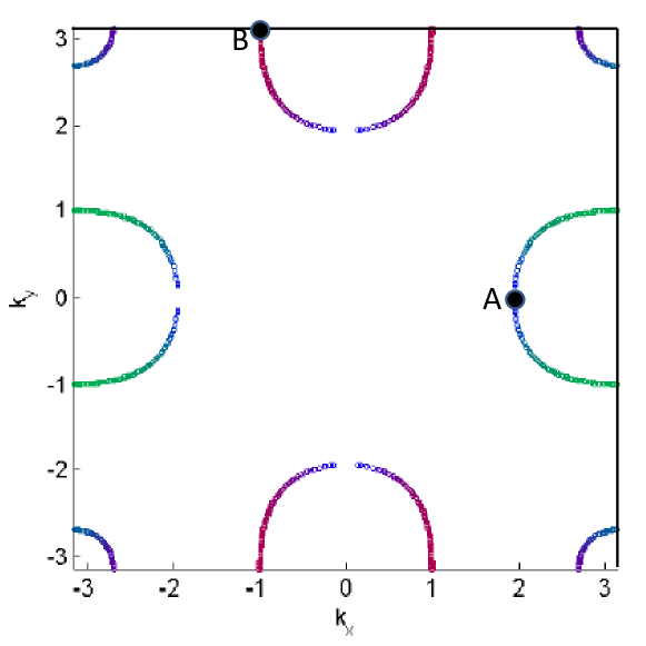
Figure 1: (color online) The Fermi surface used to represent the chalcogenides. Colors indicate the orbital components: Red $d_{xz}$, Green $d_{yz}$, and Blue=$d_{xy}$. The A and B are auxiliary labels used in Fig. 6.

Before we perform the self-consistent mean field calculation, we define the pairing order parameters as follows: in real space, the pairings on two NN bonds and two NNN bonds are represented by $\Delta^{\alpha}_{x}=J_{1}<b_{\alpha,r,r+x}>$, $\Delta^{\alpha}_{y}=J_{1}<b_{\alpha,r,r+y}>$, $\Delta^{\alpha}_{x+y}=J_{2}<b_{\alpha,r,r+x+y}>$ and $\Delta^{\alpha}_{x-y}=J_{2}<b_{\alpha,r,r+x+y}>$, where $\alpha$ denotes the orbital index and $x,y$ are the two unit lattice vectors. We only consider intra-orbital pairing and ignore inter-orbital pairing which is very small as shown in previous calculationsseo2008 . Considering the $C_{4}$ symmetry of the lattice, we can classify the pairing symmetries according to the one-dimensional irreducible representations of the $C_{4}$ symmetry. Since the pairing is a spin singlet, we can classify them as follows: an order parameter is of A-type (B-type) if it is even (odd) under a 90-degree rotation. This classification leads to six candidate pairings with A-symmetry and another six candidates with B-symmetry as the SC pairings include NN from $J_{1}$ and NNN from $J_{2}$ bonds, which manifests as the A-type symmetry

$$\Delta^{A}_{NN,s} = (\Delta^{xz}_{x}+\Delta^{xz}_{y}+\Delta^{yz}_{x}+\Delta^{yz}_{y})/4,$$

$$\Delta^{A}_{NN,d} = (\Delta^{xz}_{x}-\Delta^{xz}_{y}-\Delta^{yz}_{x}+\Delta^{yz}_{y})/4,$$

$$\Delta^{A}_{NNN,s} = (\Delta^{xz}_{x+y}+\Delta^{xz}_{x-y}+\Delta^{yz}_{x+y}+\Delta^{yz}_{x-y})/4,$$

$$\Delta^{A}_{NNN,d} = (\Delta^{xz}_{x-y}-\Delta^{xz}_{x+y}+\Delta^{yz}_{x+y}-\Delta^{yz}_{x-y})/4,$$

$$\Delta^{xy}_{NN,s} = (\Delta^{xy}_{x}+\Delta^{xy}_{y})/2,$$

$$\Delta^{xy}_{NNN,s} = (\Delta^{xy}_{x+y}+\Delta^{xy}_{x-y})/2.$$ (7)

and the B-type symmetry

$$\Delta^{B}_{NN,s} = (\Delta^{xz}_{x}+\Delta^{xz}_{y}-\Delta^{yz}_{x}-\Delta^{yz}_{y})/4,$$

$$\Delta^{B}_{NN,d} = (\Delta^{xz}_{x}-\Delta^{xz}_{y}+\Delta^{yz}_{x}-\Delta^{yz}_{y})/4,$$

$$\Delta^{B}_{NNN,s} = (\Delta^{xz}_{x+y}+\Delta^{xz}_{x-y}-\Delta^{yz}_{x+y}-\Delta^{yz}_{x-y})/4,$$

$$\Delta^{B}_{NNN,d} = (\Delta^{xz}_{x-y}-\Delta^{xz}_{x+y}-\Delta^{yz}_{x+y}+\Delta^{yz}_{x-y})/4,$$

$$\Delta^{xy}_{NN,d} = (\Delta^{xy}_{x}-\Delta^{xy}_{y})/2,$$

$$\Delta^{xy}_{NNN,d} = (\Delta^{xy}_{x-y}-\Delta^{xy}_{x+y})/2.$$ (8)

In reciprocal lattice space, the mean-field Hamiltonian is given by

$$\hat{H}=\sum_{k}\left(\begin{array}[]{cc}\hat{T}(k)&\hat{\Delta}(k)\\ \hat{\Delta}^{\dagger}(k)&-\hat{T}^{\star}(-k)\\ \end{array}\right),$$ (11)

where

$$\hat{\Delta}(k)=\left(\begin{array}[]{ccc}\Delta_{11}(k)&0&0\\ 0&\Delta_{22}(k)&0\\ 0&0&\Delta_{33}(k)\\ \end{array}\right),$$ (15)

and

$$\Delta_{11}(k) = (\Delta_{NN,s}^{A}+\Delta^{B}_{NN,s})(\cos(k_{x})+\cos(k_{y}))+(\Delta_{NN,d}^{A}+\Delta^{B}_{NN,d})(\cos(k_{x})-\cos(k_{y}))$$

$$+2(\Delta_{NNN,s}^{A}+\Delta^{B}_{NNN,s})\cos(k_{x})\cos(k_{y})+2(\Delta_{NNN,d}^{A}+\Delta^{B}_{NNN,d})\sin(k_{x})\sin(k_{y}),$$

$$\Delta_{22}(k) = (\Delta_{NN,s}^{A}-\Delta^{B}_{NN,s})(\cos(k_{x})+\cos(k_{y}))+(\Delta_{NN,d}^{B}-\Delta^{A}_{NN,d})(\cos(k_{x})-\cos(k_{y}))$$

$$+2(\Delta_{NNN,s}^{A}-\Delta^{B}_{NNN,s})\cos(k_{x})\cos(k_{y})+2(\Delta_{NNN,d}^{B}-\Delta^{A}_{NNN,d})\sin(k_{x})\sin(k_{y}),$$

$$\Delta_{33}(k) = \Delta^{xy}_{NN,s}(\cos(k_{x})+\cos(k_{y}))+\Delta^{xy}_{NN,d}(\cos(k_{x})-\cos(k_{y}))+2\Delta^{xy}_{NNN,s}\cos(k_{x})\cos(k_{y})$$ (16)

$$+2\Delta^{xy}_{NNN,d}\sin(k_{x})\sin(k_{y}).$$

We emphasize that in above definitions the symbols $s$ and $d$ merely represent the geometric factor of pairing in $k$-space, and do not correspond to whether pairing is even or odd under a 90-degree rotation in a multi-orbital system. In general, there are more than one self-consistent set of $\{\Delta\}$’s as self-consistent meanfield solutions. The free energies in each solution hence have to be compared to find the solution with the lowest free energy.

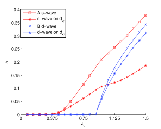
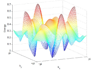
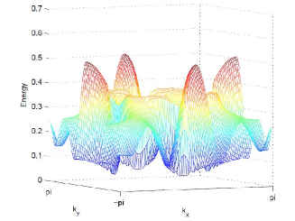
Figure 2: (color online) The mean field phase diagram along $J_{1}=0$ in the parameter space (up); the quasiparticle spectrum at $J_{2}=1$ (middle) and $J_{2}=0.75$ (bottom). At $J_{2}=1$, one can see that the quasiparticle spectrum explicitly breaks $C_{4}$ symmetry because of the mixing of A- and B-type pairing symmetries.

First consider pure NNN-pairings stemming from $J_{2}$ (this is a reasonable limit to start with since $J_{1}$ in FeTe(Se) has been shown to be ferromagnetic, thus not contributing to pairing in the singlet pairing channel). $J_{2}$ is increased from zero to $J_{2}=1.5$ while the band width is $W\sim 4$. The robust superconductivity solution with purely A-type $s$-wave pairing is obtained when $J_{2}$ is larger than $0.4$. This is to say the pairing remains the same as in iron-pnictides with the geometric factor $\cos(k_{x})\cos(k_{y})$seo2008 . The Bogoliubov particle spectrum is completely gapped in this state. When $J_{2}$ becomes larger than 1, the ground state is a mixture of A- and B-type pairings. The nonzero B-type pairings all have the geometric factor $\sin(k_{x})\sin(k_{y})$ (see the phase diagram show in Fig. 2). In the coexistence phase, the quasiparticle spectrum shows nearly gapless features at several points, and moreover, the dispersion explicitly breaks $C_{4}$ rotation symmetry (see Fig. 2 displaying the quasiparticle spectrum of the lowest branch).

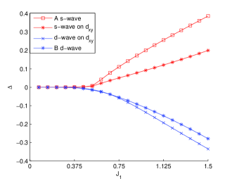
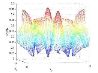
Figure 3: (color online) The mean field phase diagram along $J_{2}=0$ in the parameter space (up); the quasiparticle spectrum at $J_{1}=0.75$ (bottom). At $J_{1}=0.75$ one can see that the quasiparticle spectrum explicitly breaks the $C_{4}$ symmetry because of the mixing of A- and B-type pairing symmetries.

Second, we study the phase diagram when only (antiferromagnetic) $J_{1}$ is present. In this case, only NN pairings are nonzero and there are six SC gaps. We increase $J_{1}$ from $J_{1}=0$ to $J_{1}=1.5$ where the band width is $W\sim 4$. The SC order becomes non-zero from $J_{1}=0.4$ on. However, in this case, the B-type SC order arises slightly earlier than A-type SC order. The ground state is always a mixture of A- and B-type pairings. The two leading orders are A-type $s$-wave and B-type $d$-wave in $xz,yz$ orbitals while the sub-leading ones are $s$- and $d$-waves in the $xy$ orbitals (Fig. 3). Due to strong mixing of A- and B-type pairings, the quasiparticle spectrum is very anisotropic. It is, however, still nodeless, in contrast to a pure $s$-wave pairing $\cos(k_{x})+\cos(k_{y})$ where there are nodesThomale2010asp on the electron pockets (see Fig. 3).

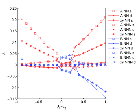
Figure 4: (color online) The mean field phase diagram with $J_{1}+J_{2}=1$ in the parameter space.

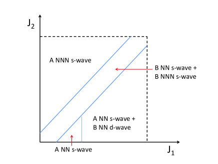
Figure 5: (color online) A schematic phase diagram for the model (11) within $0<J_{1},J_{2}<1$.

Finally, for $J_{1}$ and $J_{2}$ antiferromagnetic, we fix $J_{1}+J_{2}=1$ and change $J_{1}-J_{2}$ as a parameter. We observe that NNN pairings dominate for $J_{1}-J_{2}<-0.1$ and NN pairings dominate for $J_{1}-J_{2}>0.2$ (Fig. 4). In the intermediate range, there is only weak B-type pairing. A schematic phase diagram within the range $0<J_{1},J_{2}<1$ is shown in Fig. 5.

In the whole parameter region of $(J_{1},J_{2})$, the SC order parameters always have the same sign for all three orbitals. This can be seen in Fig. 6 where the orbital resolved pairing amplitude is shown along electron pockets around $X$. This result is essentially consistent with the FRG result shown in Sec. III (Fig.12). It is, however, different from what one would expect from the very strong coupling limit: There, the strong inter-orbital repulsion favors different signs of pairing for the $d_{xy}$ orbital and the $d_{xz/yz}$ orbitalsLu2010 . Some quantitative differences between Fig. 6 and Fig. 12 may be explained as the incompleteness of a three-orbital model and the fact that the meanfield pairing is not constrained to the FS. In Fig. 6 we also see that the orbital resolved pairing amplitude is highly anisotropic: This is a natural reflection of different orbital composition on different parts of the Fermi surface.

Following the Fermi surface topology in Fig. 1, these mean-field results have been obtained in the case where a small electron pocket was still present at the $M$-point. For completeness of the analysis, we also adapted the parameters such that the electron pocket around the $M$ point vanishes, leaving two pockets around $X$. Without the $M$ pocket, we see that $s$-wave pairings are less favored than before, as its geometric factor is $\cos(k_{x})\cos(k_{y})$ or $\cos(k_{x})+\cos(k_{y})$, both being maximized around $M$. With the two-pocket FS, taking $J_{1}=0$ and increasing $J_{2}>0$, B-type pairings blend in at smaller $J_{2}$ than shown in Fig.2; taking $J_{2}=0$ and increasing $J_{1}>0$, A-type pairings appear at slightly larger $J_{1}$ than shown in Fig. 3. The main features still remain unchanged. These trends are in accordance with the FRG studies in the following section.

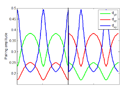
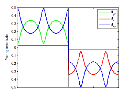
Figure 6: (color online) The orbital resolved pairing amplitude on the FS for a typical $s$-wave ($d$-wave) pairing state in the upper (lower) panel, calculated within meanfield approximation. The interaction parameters are $J_{1}=0$, $J_{2}=0.8$ for the upper panel and $J_{1}=0.5$, $J_{2}=0$ for the lower panel. In the left half of these figures, the k-point traces the electron pocket around $X$-point counterclockwise from point A in Fig. 1 and in the right half, it traces the electron pocket around the $Y$-point counterclockwise from point B in Fig. 1.

III FRG analysis

To substantiate the mean field results above, we employ functional renormalization group (FRG)zanchi-00prb13609 ; halboth-00prb7364 ; honerkamp-01prb035109 to further investigate the pairing symmetry of the $\tilde{t}$-$J_{1}$-$J_{2}$ model. As an unbiased resummation scheme of all channels, the FRG has been extended and amply employed to the multi-band case of iron pnictides. More details can be found in Refs. Wang2008a, ; platt-09njp055058, ; Thomale2009, ; Thomale2010asp, . The conventional starting point for the FRG are bare Hubbard-type interactions which develop different Fermi surface instabilities as higher momenta are integrated out when the cutoff of the theory flows to the Fermi surface. To address the special situation found in the chalcogenides where the Fe-Se coupling is strong, not only local, but also further neighbor interaction terms would have to be taken into account: in our FRG setup, the onsite Hubbard-type interactions of the same type as used in the study of pnictides triggers no instability at reasonable critical scales. This suggests already at this stage that the chalcogenides may necessitate a perspective beyond pure weak coupling. In addition, the total parameter space of bare interactions is large and constrained RPA parameters are not yet available for this class of materials. For the purpose of our study, we hence constrain ourselves to the $\tilde{t}$-$J_{1}$-$J_{2}$ model from the outset. This implies that the pairing interaction is already attractive on the bare level, and a development of an SC instability is expected as the physics is dominated by the pairing channel. Still, we can employ FRG to investigate the properties and competition of different SC pairing symmetries for the chalcogenides for different $(J_{1},J_{2})$ regimes.

Within FRG, we consider general $J_{1}$-$J_{2}$ interactions which are not limited to the spins in the same orbital:

$$H = J_{1}\sum_{\langle i,j\rangle}\sum_{a,b}(\mathbf{S}_{ia}\cdot\mathbf{S}_{jb}-\frac{1}{4}n_{ia}n_{jb})$$

$$+ J_{2}\sum_{\langle\langle i,j\rangle\rangle}\sum_{a,b}(\mathbf{S}_{ia}\cdot\mathbf{S}_{jb}-\frac{1}{4}n_{ia}n_{jb}).$$

The kinetic theory will differ in the various cases studied below. For all cases, we will study the full 5-band model incorporating all Fe $d$ orbitals. Concerning the discretization of the BZ, the RG calculations were performed with 8 patches per pocket, and a $10_{\text{radius}}\times 3_{\text{angle}}$ mesh on each patch. (This moderate resolution is convenient to scan wide ranges of the interaction parameter space; we checked that increasing the BZ resolution did not qualitatively change our findings.) The output of the RG calculation is the four-point vertex on the Fermi surfaces: $V_{\Lambda}(\boldsymbol{k}_{1},n_{1};\boldsymbol{k}_{2},n_{2};\boldsymbol{k}_{3},n_{3};\boldsymbol{k}_{4},n_{4})c_{\boldsymbol{k}_{4}n_{4}s}^{\dagger}c_{\boldsymbol{k}_{3}n_{3}\bar{s}}^{\dagger}c_{\boldsymbol{k}_{2}n_{2}s}^{\phantom{\dagger}}c_{\boldsymbol{k}_{1}n_{1}\bar{s}}^{\phantom{\dagger}},$ where the flow parameter is the IR cutoff $\Lambda$ approaching the Fermi surface, and with $\boldsymbol{k}_{1}$ to $\boldsymbol{k}_{4}$ the incoming and outgoing momenta. We only find singlet pairing to be relevant for the scenarios studied by us: $\sum_{\boldsymbol{k},\boldsymbol{p}}V_{\Lambda}(\boldsymbol{k},\boldsymbol{p})[\hat{O}^{\dagger}_{\boldsymbol{k}}\hat{O}^{\phantom{\dagger}}_{\boldsymbol{p}}]$, where $\hat{O}^{\text{SC}}_{\boldsymbol{k}}=c_{\boldsymbol{k},\uparrow}c_{-\boldsymbol{k},\downarrow}$. We decompose the pairing channel into eigenmodes,

$$V^{\text{SC}}_{\Lambda}(\boldsymbol{k},-\boldsymbol{k},\boldsymbol{p})=\sum_{i}c_{i}^{\text{SC}}(\Lambda)f^{\text{SC},i}(\boldsymbol{k})^{*}f^{\text{SC},i}(\boldsymbol{p}),$$ (17)

and obtain the band-resolved form factors of the leading and subleading SC eigenmode (i.e. largest two negative eigenvalues). This way we are able to discuss the interplay of $d$-wave and $s$-wave as well as the degree of form factor anisotropy for a given setting of $(J_{1},J_{2})$. Comparing divergence scales $\Lambda_{c}$ gives us the possibility to investigate the relative change of $T_{c}$ as a function of $(J_{1},J_{2})$. Furthermore, we also investigate the orbital-resolved pairing modesThomale2010asp by decomposing the orbital four point vertex

$$V^{\text{orb}}_{c,d\rightarrow a,b} = \sum_{n_{1},\ldots,n_{4}=1}^{5}\Big{\{}V_{\Lambda}(\boldsymbol{k}_{1},n_{1};\boldsymbol{k}_{2},n_{2};\boldsymbol{k}_{3},n_{3};\boldsymbol{k}_{4},n_{4})$$ (18)

$$\times u^{*}_{an_{1}}(\boldsymbol{k}_{1})u^{*}_{bn_{2}}(\boldsymbol{k}_{2})u_{cn_{3}}(\boldsymbol{k}_{3})u_{dn_{4}}(\boldsymbol{k}_{4})\Big{\}},$$

where the $u$’s denote the different orbital components of the band vectors. By investigating the intraorbital SC pairing modes in (18), we make contact to the findings from the previous mean field analysis.

III.1 Two-pocket scenario

We start by studying the 5-band model suggested before by Maier et al.Maier2011 . There are only two electron pockets at the $X$ point of the unfolded Brillouin zone closely resembling the Fermi surface topology and orbital content employed for our mean-field analysis (Fig. 7).

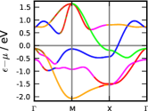
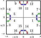
Figure 7: (color online) The spectrum and the Fermi surfaces of the band structure proposed by Maier et al. Maier2011 , colored according to the dominant orbital content. The color code is red $d_{xz}$, green $d_{yz}$, blue $d_{xy}$, orange $d_{x^{2}-y^{2}}$ and magenta $d_{3z^{2}-r^{2}}$. The numbered crosses show the center of Fermi surface patches used in the FRG calculations.

The RG flow and the form factors of the leading diverging channels are shown in Fig. 8 for dominant $J_{2}$ and in Fig. 9 for dominant $J_{1}$. As stated before, the pairing interaction is already present at the bare level in the model so that we achieve comparably fast instabilities as the cutoff is flowing towards the Fermi surface. As found in Ref. seo2008, , the dominant $J_{2}$ scenario exhibits a leading $s$-wave $\cos k_{x}\cos k_{y}$ form factor which causes the same sign on both electron pockets (blue dots in Fig. 8). The subleading form factor is found to be of $d$-wave $\cos k_{x}-\cos k_{y}$ type, changing sign from one electron pocket to the other. The inverse situation is found for dominant $J_{1}$. As shown in Fig. 9, the $d$-wave $\cos k_{x}-\cos k_{y}$ form factor establishes the leading instability. As before, the form factor does not cross zero related to nodeless SC for this parameter setting.

With only pairing information available on the limited number of sampling points along FS, it is impossible to obtain as in the mean-field analysis the superconducting gap in the whole BZ. For illustration, a mixture of a small A-type NNN d-wave pairing and large A-type NNN s-wave pairing is indistinguishable from a pure A-type NNN s-wave pairing; a mixed state of a small B-type NN $s$-wave pairing plus a large B-type NN $d$-wave pairing, and a state with pure B-type NN $d$-wave pairing show little difference if one compares the gap on a few points along the Fermi surfaces. For this reason, the symbol $s_{x^{2}y^{2}}$ used in this section refers to a pairing consisting of a large A-type NNN $s$-wave pairing and possible small components of A-type NNN $d$-wave pairing or A-type NN $s$/$d$-wave pairing. In turn, the symbol $d_{x^{2}-y^{2}}$ refers to a pairing made up with a large B-type NN $d$-wave pairing and possible small components of B-type NN $s$-wave pairing or B-type NNN $s$/$d$-wave pairing.

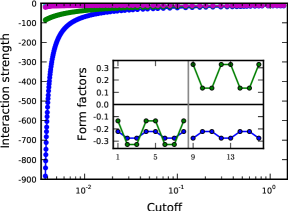
Figure 8: (color online) Typical RG flows and the superconducting gaps associated with the Fermi surfaces for the two-pocket scenario with $(J_{1},J_{2})=(0.1,0.5)$ eV. Leading form factor is denoted in blue, sub-leading form factor in green.

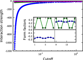
Figure 9: (color online) Typical RG flows and the superconducting gaps associated with the Fermi surfaces for the two-pocket scenario with $(J_{1},J_{2})=(0.5,0.1)$ eV. Leading form factor is denoted in blue, sub-leading form factor in green.

We have scanned a large range of $(J_{1},J_{2})$. For each setup we have obtained $\Lambda_{c}$ as well as the ratio of the instability eigenvalues between $s$-wave and $d$-wave in the pairing channel (encoded by the two-color circles shown in Fig. 10). The FRG result is qualitatively consistent with the mean field analysis. In the antiferromagnetic sector, the $s$-wave wins for dominant $J_{2}$ while the $d$-wave wins wins for dominant $J_{1}$. For ferromagnetic $J_{1}$ corresponding to the situation in chalcogenides, we find a robust preference of $s$-wave pairing. The anisotropy of the s-wave gap around the pockets in the FRG calculation is also qualitatively consistent with the meanfield result. The gap on the Fermi surfaces with $d_{xy}$ orbital character is smaller than the gap on those with $d_{xz,yz}$ orbital character.

The predictions from the mean field analysis are further confirmed for the mixed phase regime where $s$-wave and $d$-wave coexist in the mean field solution. In FRG, one of these instabilities will always be slightly preferred; still, when both instabilities diverge in very close proximity to each other, this regime behaves similarly to the coexistence phase. For illustration, in Fig. 11 we have plotted the dependence of $\Lambda_{c}$ on $J_{1}-J_{2}$, with $J_{1}+J_{2}$ fixed to $0.7$ eV; there is a clear reduction of the critical scale (and thus the transition temperature) when there is a strong competition between $s$- and $d$-wave channels.

Following (18) we also analyze the orbital decomposition of the SC pairing from FRG (Fig. 12). We constrain ourselves to the most relevant three orbitals $d_{xy}$, $d_{xz}$, and $d_{yz}$. In particular, we observe that the SC orbital pairing induces the same sign for all three dominant orbital modes, in correspondence with the mean field analysis presented before.

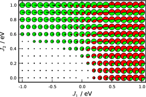
Figure 10: (color online) The phase diagram of the two-pocket model. Each pie shows the relative strengths of the two leading pairing channels, with the radius proportional to $[8+\log_{10}(\Lambda_{c}/\text{eV})]^{2}$. The color code for pairing symmetries is green $s_{x^{2}y^{2}}$ and red $d_{x^{2}-y^{2}}$.

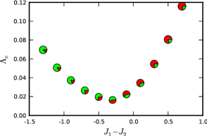
Figure 11: (color online) The variation of the critical scale $\Lambda_{c}$ along a line through parameter space which interpolates between $s$ and $d$ wave. A minimum is visible for comparable ordering tendency in $s$-wave and $d$-wave. See the caption of Fig. 10 for more details on the pie charts.

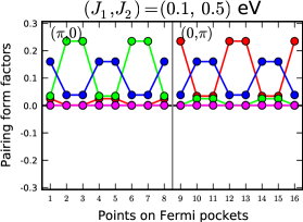
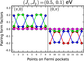
Figure 12: (color online) The orbital-resolved pairing form factors of two typical RG flows. The upper resides in the dominant $s$-wave and the lower in the $d$-wave regime. The color code is the same as in Fig. 7, i. e. red $d_{xz}$, green $d_{yz}$, blue $d_{xy}$, orange $d_{x^{2}-y^{2}}$ and magenta $d_{3z^{2}-r^{2}}$.

III.2 Three-pocket scenario

Recent ARPES datasergei on the chalcogenides may suggest the existence of a shallow flat pocket around the $\Gamma$ point (the location, and especially the $k_{z}$ position of such a pocket are still under debate). By tuning parameters, we have obtained in the previous section a three-orbital model that has an additional electron-pocket around $M$-point in the unfolded BZ.

In our FRG approach we can take a more profound microscopic perspective on this issue. From the true band structure calculations at hand for the chalcogenides, we consider it unlikely that it will be a hole band regularized up towards the Fermi surface.

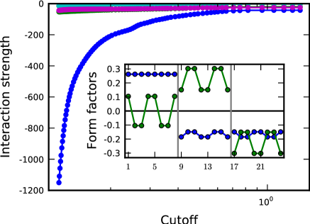
Figure 13: (color online) Typical RG flows and the superconducting gaps associated with Fermi surface for the three-pocket scenario with $(J_{1},J_{2})=(0.2,0.8)$ eV. Leading form factor is denoted in blue, sub-leading form factor in green.

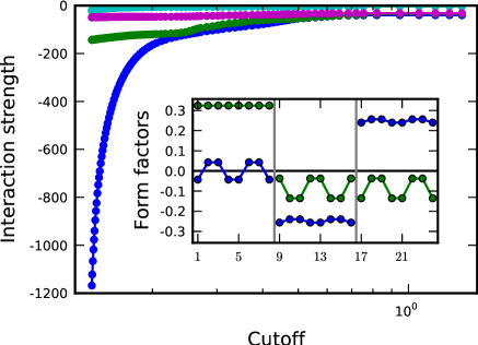
Figure 14: (color online) Typical RG flows and the superconducting gaps associated with Fermi surface for the three-pocket scenario with $(J_{1},J_{2})=(0.9,0.3)$ eV. Leading form factor is denoted in blue, sub-leading form factor in green.

Instead, we investigate the effect of a possible electron band at the $\Gamma$ point in the unfolded Brillouin zone. This is suggested from the folded 10-band calculations, where one electron-type band closely approaches the Fermi level around the $\Gamma$ pointMaier2011 . This band should be very flat and shallow. From the weak coupling perspective of particle-hole pairs created around the Fermi surfaces, this will probably have a small effect: particle-hole pairs will only be created up to energy scales of the depth of the electron band at the $X$ point below the Fermi surface, providing some hole-type phase space for the electron band at $\Gamma$. In a $(J_{1},J_{2})$ picture, however, this may still significantly promote scattering along $\Gamma\leftrightarrow X$, which may further stabilize the $s$-wave phase regime. We have hence developed a modified band structure designed for this scenario. There, we have bent down the band dominated by $d_{xy}$ in the two-pocket model band structureMaier2011 without changing its band vector and created an electron pocket around $\Gamma$, accordingly of mainly $d_{xy}$ orbital content (Fig. 15). The band bending was achieved by

$$H\rightarrow H+\sum_{\mathbf{k,a,b,s}}\xi(\mathbf{k})c_{\mathbf{k}as}^{\dagger}u_{a}(\mathbf{k})u^{*}_{b}(\mathbf{k})c_{\mathbf{k}bs},$$

where $u(\mathbf{k})$ is the eigenvector of the band dominated by $d_{xy}$. The shift of energy $\xi(\mathbf{k})$ was intentionally chosen such that the $\Gamma$ pocket exhibits some nesting with the $X$ electron pockets.

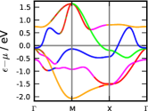
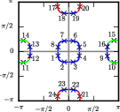
Figure 15: (color online) The band structure and the Fermi surfaces of the modified band structure, colored according to the dominant orbital content. The color code is red $d_{xz}$, green $d_{yz}$, blue $d_{xy}$, orange $d_{x^{2}-y^{2}}$ and magenta $d_{3z^{2}-r^{2}}$. The numbered crosses show the center of Fermi surface patches used in the FRG calculations.

The phase diagram is shown in Fig. 16. FRG results for typical scenario for the $s$-wave and $d$-wave regime are shown in Fig. 13 and Fig. 14, respectively. As suspected, the additional pocket strengthens the tendency to form an $s$-wave in the system, aside from exhibiting an additional constant $s$-wave instability in a small regime for dominant $J_{1}$.

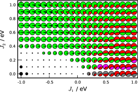
Figure 16: (color online) The phase diagram of the three-pocket model. Here we are able to resolve the $s$-wave channel into constant $s$-wave (grey), extended $s_{x^{2}y^{2}}$-wave (green), and the nodal $s_{x^{2}+y^{2}}$-wave (purple). Parameter sets with $J_{1}\sim-1$ and $J_{2}\sim 0$ have highly oscillating form factors which are due to artifacts in the calculation; the triplet channel would have to be considered in these cases.

IV Discussion

The above calculations demonstrate that the $s$-wave pairing symmetry is always robust if the AFM NNN $J_{2}$ is strong while a $d$-wave pairing can be strong if $J_{1}$ is AFM for the electron overdoped region. Moreover, if both of them are AFM, there is strong competition between the $s$-wave and $d$-wave pairing. When there are hole pockets, as shown beforeseo2008 , even in a range of $J_{1}\sim J_{2}$, the contribution to pairing from $J_{1}$ is much weaker than the one from $J_{2}$. In that case, an AFM $J_{1}$ will not generate strong $d$-wave pairing so that the $s$-wave wins easily. From neutron scattering experiments, it has been shown that a major difference between iron-pnictides and iron-chalcogenides is that the NN coupling $J_{1}$ change from AFM in the formerZhaojun2008 ; Zhaoj2009 to FM in the latterLip2011 . In fact, $J_{1}$ is rather strongly FM in the latter, which explains the high magnetic transition temperature ($500$ K) in the 245 vacancy ordering state as shown in Ref. Fang2011d, . Combining these results, we can partially answer the question regarding the different behaviors between iron-pnictides and iron-chacogenides in the electron-overdoped region: why can the high SC transition temperature be achieved in the latter, but not in the former? Since $J_{1}$ in iron-pnictides is AFM while it is FM in iron-chacogenides, $J_{1}$ will weaken the SC pairing in the former but not in the latter.

A few remarks regarding this work follow: (i) Our mean-field result is qualitatively consistent with the results from a similar model with five orbitalsYu2011 ; Yu2011mott ; yugossi . The critical difference is regarding $J_{1}$ being FM, and has not been addressed previously; (ii) $s$-wave pairing symmetry has also been obtained in Refs. Zhou2011a, ; Youy2011, ; wang2011a, . However, the $s$-wave pairing only shows up either in a narrow region or with drastically different parameter settings. Therefore, the $s$-wave is not robust from a microscopic point of view. Instead, the $d$-wave is a robust result in these studies. Still, even the $d$-wave pairing strength based on the scattering between two electron pockets is generally weak, as specifically discussed inYu2011 , which is another difficulty for this type of mechanism. (iii) Our results suggest that there is no difference between iron-pnictides and iron-chalcogenides in terms of pairing symmetry. Both of them are dominated by $s$-wave pairing. If both hole and electron pockets are present, the signs of the SC order in hole and electron pockets are opposite, namely $s^{\pm}$. However, the mechanism causing $s^{\pm}$ is different in the weak and strong coupling approach. In the weak coupling approach, the sign change is due to the scattering between the hole and electron pockets while in the strong coupling approach, the sign change is due to the form factor of the SC order parameters which is specified to be $\cos k_{x}\cos k_{y}$ since the pairing mainly originates from the AFM $J_{2}$. Therefore, to obtain $s^{\pm}$ pairing symmetry, the existence of both hole and electron pockets is necessary in the weak coupling approach, but not in the strong coupling one. (iv) The reason that the superconductivity vanishes in the iron pnictides in the electron overdoped region is not solely due to the competition between $s$-wave and $d$-wave pairing symmetry. It is also due to the weakening of local magnetic exchange coupling themselves and the reduction of band width renormalization. (v) The prospective experimental confirmation of $s$-wave pairing symmetry in $\text{KFe}_{2}\text{Se}_{2}$ will support that superconductivity in iron-based superconductors might be explained by local AFM exchange couplings. (vi) Neutron scattering also suggests that there is significant AFM exchange coupling between two third nearest neighbor sites, i.e. $J_{3}$Lip2011 ; Fang2009b . The existence of $J_{3}$ will further enhance the $s$-wave pairing since it generates pairing form factors as $\cos 2k_{x}+\cos 2k_{y}$ in reciprocal space which in turn can enhance the pairing at the electron pockets.

V Conclusion

In summary, we have shown that the pairing symmetry in electron-overdoped iron-chalcogenides is a robust $s$-wave. The fact that the NN magnetic exchange coupling is FM, which diminishes the possibility of $d$-wave pairing symmetry in these materials. From a unified perspective of high-$T_{c}$ cuprates and high-$T_{c}$ chalcogenides, the NN AFM exchange coupling gives rise to the robust $d$-wave pairing in the cuprates while the NNN AFM exchange coupling gives rise to the robust $s$-wave pairing in iron-based chalcogenide superconductors.

- (1) J. Guo, S. Jin, G. Wang, S. Wang, K. Zhu, T. Zhou, M. He, and X. Chen, Phy. Rev. B. 82, 180520 (2010).
- (2) M. Fang, H. Wang, C. Dong, Z. Li, C. Feng, J. Chen, and H. Q. Yuan, arXiv:1012.5236 (2010).
- (3) R. H. Liu, X. G. Luo, M. Zhang, A. F. Wang, J. J. Ying, X. F. Wang, Y. J. Yan, Z. J. Xiang, P. Cheng, G. J. Ye, Z. Y. Li, and X. H. Chen, arXiv:1102.2783 (2011).
- (4) D. N. Basov and A.V. Chubukov, Nature Physics 7, 273 (2011).
- (5) Y. Zhang, L. X. Yang, M. Xu, Z. R. Ye, F. Chen, C. He, J. Jiang, B. P. Xie, J. J. Ying, X. F. Wang, X. H. Chen, J. P. Hu, and D. L. Feng, Nature Materials (2010).
- (6) X. Wang, T. Qian, P. Richard, P. Zhang, J. Dong, H. Wang, C. Dong, M. Fang, and H. Ding, Europhys. Lett. 93, 57001 (2011).
- (7) D. Mou et al., Phys. Rev. Lett. 106, 107001 (2011).
- (8) C. Cao and J. Dai, arXiv:1012.5621 (2010).
- (9) L. Zhang and D. J. Singh, Phys.Rev.B 79, 094528 (2009) 79, 094528 (2009).
- (10) X. Yan, M. Gao, Z. Lu, and T. Xiang, arXiv:1012.5536 (2010).
- (11) K. Seo, B. A. Bernevig, and J. Hu, Phys. Rev. Lett. 101, 206404 (2008).
- (12) C. Fang, H. Yao, W.-F. Tsai, J. Hu, and S. A. Kivelson, Phys. Rev. B 77, 224509 (2008).
- (13) F. Wang, H. Zhai, Y. Ran, A. Vishwanath, and D.-H. Lee, Phys. Rev. Lett. 102, 047005 (2008).
- (14) I. I. Mazin, M. D. Johannes, L. Boeri, K. Koepernik, and D. J. Singh, Phys. Rev. B 78, 085104 (2008).
- (15) A. Chubukov, D. Efremov, and I. Eremin, Phys. Rev. B 78, 134512 (2008).
- (16) T. A. Maier and D. J. Scalapino, Phys. Rev. B 78, 020514 (2008).
- (17) R. Thomale, C. Platt, J. Hu, C. Honerkamp, and B. A. Bernevig, Phy. Rev. B 80, 180505(R) (2009).
- (18) R. Thomale, C. Platt, W. Hanke, J. Hu, and B. A. Bernevig, arXiv:1101.3593 (2011).
- (19) Q. Si and E. Abrahams, Phys. Rev. Lett. 101, 076401 (2008).
- (20) M. Berciu, I. Elfimov, and G. A. Sawatzky, arXiv0811.0214B (2008).
- (21) W.-Q. Chen, K.-Y. Yang, Y. Zhou, and F.-C. Zhang, Phys. Rev. Lett. 102, 047006 (2009).
- (22) J. Dai, Q. Si, J.-X. Zhu, and E. Abrahams, PNAS 106, 4118 (2009).
- (23) S.-P. Kou, T. Li, and Z.-Y. Weng, Europhys. Lett. 88, 17010 (2008).
- (24) K. Haule, J. H. Shim, and G. Kotliar, Phys. Rev. Lett. 100, 226402 (2008).
- (25) K. Haule and G. Kotliar, New J. of Phys. 11, 025021 (2009).
- (26) J. Wu and P. Phillips, Phys. Rev. B 79, 092502 (2009).
- (27) M. Daghofer, A. Moreo, J. A. Riera, E. Arrigoni, D. J. Scalapino, and E. Dagotto, Phys. Rev. Lett. 101, 237004 (2008).
- (28) V. Mishra, G. Boyd, S. Graser, T. Maier, P. J. Hirschfeld, and D. J. Scalapino, Phys. Rev. B 79, 094512 (2009).
- (29) P. A. Lee and X.-G. Wen, Phys. Rev. Lett. 78, 144517 (2008).
- (30) V. Cvetkovic and Z. Tesanovic, Eur. Phys. Lett. 85, 37002 (2009).
- (31) K. Kuroki, S. Onari, R. Arita, H. Usui, Y. Tanaka, H. Kontani, and H. Aoki, Phys. Rev. Lett. 101, 087004 (2008).
- (32) F. Wang, H. Zhai, and D.-H. Lee, Europhys. Lett. 85, 37005 (2009).
- (33) S. Graser, T. A. Maier, P. J. Hirschfeld, and D. J. Scalapino New J. Phys. 11, 025016 (2009).
- (34) S. Graser, A. F. Kemper, T. A. Maier, H.-P. Cheng, P. J. Hirschfeld, and D. J. Scalapino, arXiv:1003.0133.
- (35) A. Nicholson, W. Ge, X. Zhang, J. Riera, M. Daghofer, A. M. Oles, G. B. Martins, A. Moreo, and E. Dagotto, arXiv:1102.1445
- (36) J. Kang and Z. Tesanovic, Phys. Rev. B 83, 020505 (2011).
- (37) S. Maiti, A. V. Chubukov, arXiv:1104.2923.
- (38) T.A. Maier, S. Graser, P.J. Hirschfeld, and D.J. Scalapino, arXiv:1103.0688.
- (39) R. Thomale, C. Platt, W. Hanke, and A. Bernevig, arXiv:1002.3599.
- (40) V. Stanev, B. Alexandrov, P. Nikolic, and Z. Tesanovic, arXiv:1006.0447.
- (41) C. Platt, R. Thomale, and W. Hanke, arXiv:1012.1763.
- (42) S.Maiti, M.M. Korshunov, T.A. Maier, P.J. Hirschfeld, and A.V. Chubukov, arXiv:1104.1814.
- (43) Y.-Z. You, H. Yao, and D.-H. Lee, arXiv:1103.3884 .
- (44) T. A. Maier, S. Graser, P. J. Hirschfeld, and D. J. Scalapino, arXiv:1101.4988 (2011).
- (45) J.-X. Zhu, R. Yu, A. V. Balatsky, and Q. Si, arXiv:1103.3509.
- (46) M. M. Parish, J. Hu, and B. A. Bernevig, Phys. Rev. B 78, 144514 (2008).
- (47) O. J. Lipscombe, G. F. Chen, C. Fang, T. G. Perring, D. L. Abernathy, A. D. Christianson, T. Egami, N. Wang, J. Hu, and P. Dai, Phys. Rev. Lett. 106, 057004 (2011).
- (48) F. Ma, W. Ji, J. Hu, Z.-Y. LU, and T. Xiang, Phys. Rev. Lett. 102, 177003 (2009).
- (49) C. Fang, B. Andrei Bernevig, and J. Hu, Europhys. Lett. 86, 67005 (2009).
- (50) W. Bao, Q. Huang, G. F. Chen, M. A. Green, D. M. Wang, J. B. He, X. Q. Wang, and Y. Qiu, arXiv:1102.0830 (2011).
- (51) C. Fang, B. Xu, P. Dai, T. Xiang, and J. Hu, arXiv:1103.4599 (2011).
- (52) M. Daghofer, A. Nicholson, A. Moreo, and E. Dagotto, Phys. Rev. B 81 014511 (2010).
- (53) D. Zanchi and H. J. Schulz, Phys. Rev. B 61, 13609 (2000).
- (54) C. J. Halboth and W. Metzner, Phys. Rev. B 61, 7364 (2000).
- (55) C. Honerkamp, M. Salmhofer, N. Furukawa, and T. M. Rice, Phys. Rev. B 63, 035109 (2001).
- (56) C. Platt, C. Honerkamp, and W. Hanke, New J. Phys. 11, 055058 (2009).
- (57) S. Borisenko, unpublished.
- (58) J. Zhao, D.-X. Yao, S. Li, T. Hong, Y. Chen, S. Chang, W. Ratcliff, II, J. W. Lynn, H. A. Mook, G. F. Chen, J. L. Luo, N. L. Wang, E. W. Carlson, J. Hu, and P. Dai, Phys. Rev. Lett. 101, 167203 (2008).
- (59) J. Zhao, D. T. Adroja, D.-X. Yao, R. Bewley, S. Li, X. F. Wang, G. Wu, X. H. Chen, J. Hu, and P. Dai, Nature Physics 5, 55 (2009).
- (60) X. Lu, Chen Fang, W.F. Tsai, Y. Jiang and J. Hu, arXiv:1012.2566 (2010).
- (61) R. Yu, P. Goswami, Q. Si, P. Nikolic, and J. Zhu, arXiv:1103.3259 (2011).
- (62) R. Yu, J. Zhu, and Q. Si, arXiv:1101.3307 (2011).
- (63) R. Yu, P. Goswami, and Q. Si, arXiv:1104.1445.
- (64) Y. Zhou, D. Xu, F. Zhang, and W. Chen, arXiv:1101.4462 (2011).
- (65) F. Wang, F. Yang, M. Gao, Z.Y. Lu, T. Xiang and D.H. Lee, Europhys. Lett 93 57003 (2011).