On the anomalous secular increase of the eccentricity of the orbit of the Moon

Abstract

A recent analysis of a Lunar Laser Ranging (LLR) data record spanning 38.7 yr revealed an anomalous increase of the eccentricity $e$ of the lunar orbit amounting to $\dot{e}_{\rm meas}=(9\pm 3)\times 10^{-12}$ yr^-1. The present-day models of the dissipative phenomena occurring in the interiors of both the Earth and the Moon are not able to explain it. In this paper, we examine several dynamical effects, not modeled in the data analysis, in the framework of long-range modified models of gravity and of the standard Newtonian/Einsteinian paradigm. It turns out that none of them can accommodate $\dot{e}_{\rm meas}$. Many of them do not even induce long-term changes in $e$; other models do, instead, yield such an effect, but the resulting magnitudes are in disagreement with $\dot{e}_{\rm meas}$. In particular, the general relativistic gravitomagnetic acceleration of the Moon due to the Earth’s angular momentum has the right order of magnitude, but the resulting Lense-Thirring secular effect for the eccentricity vanishes. A potentially viable Newtonian candidate would be a trans-Plutonian massive object (Planet X/Nemesis/Tyche) since it, actually, would affect $e$ with a non-vanishing long-term variation. On the other hand, the values for the physical and orbital parameters of such a hypothetical body required to obtain at least the right order of magnitude for $\dot{e}$ are completely unrealistic: suffices it to say that an Earth-sized planet would be at 30 au, while a jovian mass would be at 200 au. Thus, the issue of finding a satisfactorily explanation for the anomalous behavior of the Moon’s eccentricity remains open.

1 Introduction

Anderson & Nieto (2010), in a review of some astrometric anomalies recently detected in the solar system by several independent groups, mentioned also an anomalous secular increase of the eccentricity $e$ of the orbit of the Moon

$$\dot{e}_{\rm meas}=(9\pm 3)\times 10^{-12}\ {\rm yr^{-1}}$$ (1)

based on an analysis of a long LLR data record spanning 38.7 yr (16 March 1970-22 November 2008) performed by Williams & Boggs (2009) with the suite of accurate dynamical force models of the DE421 ephemerides (Folkner et al., 2008; Williams et al., 2008) including all relevant Newtonian and Einsteinian effects. Notice that eq. (1) is statistically significant at a $3\sigma-$level. The first presentation of such an effect appeared in Williams et al. (2001), in which an extensive discussion of the state-of-the-art in modeling the tidal dissipation in both the Earth and the Moon was given. Later, Williams & Dickey (2003), relying upon Williams et al. (2001), yielded an anomalous eccentricity rate as large as $\dot{e}_{\rm meas}=(1.6\pm 0.5)\times 10^{-11}$ yr^-1. Anderson & Nieto (2010) commented that eq. (1) is not compatible with present, standard knowledge of dissipative processes in the interiors of both the Earth and Moon, which were, actually, modeled by Williams & Boggs (2009). The relevant physical and osculating orbital parameters of the Earth and the Moon are reported in Table 1.

Table 1: Relevant physical and osculating orbital parameters of the Earth-Moon system. $a$ is the semimajor axis. $e$ is the eccentricity. The inclination $I$ is referred to the mean ecliptic at J2000.0. $\Omega$ is the longitude of the ascending node and is referred to the mean equinox and ecliptic at J2000.0. $\omega$ is the argument of pericenter. $G$ is the Newtonian gravitational constant. The masses of the Earth and the Moon are $M$ and $m$, respectively. The orbital parameters of the Moon were retrieved from the WEB interface HORIZONS (Author: J. Giorgini. Site Manager: D. K. Yeomans. Webmaster: A. B. Chamberlin), by JPL, NASA, at the epoch J2000.0.

$a$ (m)	$e$	$I$ (deg)	$\Omega$ (deg)	$\omega$ (deg)	$GM$ (m3 s-2)	$m/M$
$3.81219\times 10^{8}$	$0.0647$	$5.24$	$123.98$	$-51.86$	$3.98600\times 10^{14}$	$0.012$

In this paper we look for a possible candidate for explaining such an anomaly in terms of both Newtonian and non-Newtonian gravitational dynamical effects, general relativistic or not.

To this aim, let us make the following, preliminary remarks. Naive, dimensional evaluations of the effect caused on $e$ by an additional anomalous acceleration $A$ can be made by noticing that

$$\dot{e}\approx{A\over na},$$ (2)

with

$$na=1.0\times 10^{3}\ {\rm m\ s^{-1}}=3.2\times 10^{10}\ {\rm m\ yr^{-1}}$$ (3)

for the geocentric orbit of the Moon. In it, $a$ is the orbital semimajor axis, while $n\doteq\sqrt{\mu/a^{3}}$ is the Keplerian mean motion in which $\mu\doteq GM(1+m/M)$ is the gravitational parameter of the Earth-Moon system: $G$ is the Newtonian constant of gravitation. It turns out that an extra-acceleration as large as

$$A\approx 3\times 10^{-16}\ {\rm m\ s}^{-2}=0.3\ {\rm m\ yr^{-2}}$$ (4)

would satisfy eq. (1). In fact, a mere order-of-magnitude analysis based on eq. (2) would be insufficient to draw meaningful conclusions: finding simply that this or that dynamical effect induces an extra-acceleration of the right order of magnitude may be highly misleading. Indeed, exact calculations of the secular variation of $e$ caused by such putative promising candidate extra-accelerations $A$ must be performed with standard perturbative techniques in order to check if they, actually, cause an averaged non-zero change of the eccentricity. Moreover, also in such potentially favorable cases caution is still in order. Indeed, it may well happen, in principle, that the resulting analytical expression for $\left\langle\dot{e}\right\rangle$ retains multiplicative factors $1/e^{k},k=1,2,3,...$ or $e^{k},k=1,2,3...$ which would notably alter the size of the found non-zero secular change of the eccentricity with respect to the expected values according to eq. (2).

The plan of the paper is as follows. In Section 2 we deal with several long-range models of modified gravity. Section 3 analyzes some dynamical effects in terms of the standard Newtonian/Einsteinian laws of gravitation. The conclusions are in Section 4.

2 Exotic models of modified gravity

2.1 A Rindler-type acceleration

As a practical example of the aforementioned caveat, let us consider the effective model for gravity of a central object of mass $M$ at large scales recently constructed by Grumiller (2010). Among other things, it predicts the existence of a constant and uniform acceleration

$$\boldsymbol{A}=A_{\rm Rin}\boldsymbol{\hat{r}}$$ (5)

radially directed towards $M$. As shown in Iorio (2010a), the Earth-Moon range residuals $\delta\rho$ over $\Delta t=20$ yr yield the following constrain for a terrestrial Rindler-type extra-acceleration

$$A_{\rm Rin}\lesssim 5\times 10^{-16}\ {\rm m\ s^{-2}}=0.5\ {\rm m\ yr^{-2}},$$ (6)

which is in good agreement with eq. (4).

The problem is that, actually, a radial and constant acceleration like that of eq. (5) does not induce any secular variation of the eccentricity. Indeed, from the standard Gauss perturbation equation for $e$ (Bertotti et al., 2003)

$$\frac{{{d}}{e}}{{{d}}{t}}={\sqrt{1-e^{2}}\over na}\left\{A_{R}\sin f+A_{T}\left[\cos f+{1\over e}\left(1-{r\over a}\right)\right]\right\},$$ (7)

in which $f$ is the true anomaly, and $A_{R},A_{T}$ are the radial and transverse components of the perturbing acceleration $\boldsymbol{A}$, it turns out (Iorio, 2010a)

$$\Delta e=-{A_{\rm Rin}\left(1-e^{2}\right)\left(\cos E-\cos E_{0}\right)\over n^{2}},$$ (8)

where $E$ is the eccentric anomaly, so that

$$\left.\Delta e\right|_{0}^{2\pi}=0.$$ (9)

2.2 A Yukawa-type long-range modification of gravity

It is well known that a variety of theoretical paradigms (Adelberger et al., 2003; Bertolami & Páramos, 2005) allow for Yukawa-like deviations from the usual Newtonian inverse-square law of gravitation (Burgess & Cloutier, 1988). The Yukawa-type correction to the Newtonian gravitational potential $U_{\rm N}=-\mu/r$, where $\mu\doteq GM$ is the gravitational parameter of the central body which acts as source of the supposedly modified gravitational field, is

$$U_{\rm Y}=-{\alpha\mu_{\infty}\over r}\exp\left(-{r\over{\mathchoice{\mbox{l}}{\mbox{l}}{\mbox{l}}{\mbox{l}}}}\right),$$ (10)

where $\mu_{\infty}$ is the gravitational parameter evaluated at distances $r$ much larger than the scale length l.

In order to compute the long-term effects of eq. (10) on the eccentricity of a test particle it is convenient to adopt the Lagrange perturbative scheme (Bertotti et al., 2003). In such a framework, the equation for the long-term variation of $e$ is (Bertotti et al., 2003)

$$\left\langle{de\over dt}\right\rangle={1\over na^{2}}\left({1-e^{2}\over e}\right)\left({1\over\sqrt{1-e^{2}}}{\partial\mathcal{R}\over\partial\omega}-{\partial\mathcal{R}\over\partial\mathcal{M}}\right),$$ (11)

where $\omega$ is the argument of pericenter, $\mathcal{M}\doteq n(t-t_{p})=E-e\sin E$ is the mean anomaly of the test particle, and $\mathcal{R}$ denotes the average of the perturbing potential over one orbital revolution. In the case of a Yukawa-type perturbation, eq. (10) yields

$$\left\langle U_{\rm Y}\right\rangle=-{\alpha\mu_{\infty}\exp\left(-{a\over{\mathchoice{\mbox{l}}{\mbox{l}}{\mbox{l}}{\mbox{l}}}}\right)\over a}I_{0}\left({ae\over{\mathchoice{\mbox{l}}{\mbox{l}}{\mbox{l}}{\mbox{l}}}}\right),$$ (12)

where $I_{0}(x)$ is the modified Bessel function of the first kind $I_{k}(x)$ for $k=0$. An inspection of eq. (11) and eq. (12) immediately tells us that there is no secular variation of $e$ caused by an anomalous Yukawa-type perturbation which, thus, cannot explain eq. (1).

2.3 Other long-range exotic models of gravity

The previous analysis has the merit of elucidating certain general features pertaining to a vast category of long-range modified models of gravity. Indeed, eq. (11) tells us that a long-term change of $e$ occurs only if the averaged extra-potential considered explicitly depends on $\omega$ and on time through $\mathcal{M}$ or, equivalently, $E$. Actually, the anomalous potentials arising in the majority of long-range modified models of gravity are time-independent and spherically symmetric (Dvali et al., 2000; Capozziello et al., 2001; Capozziello & Lambiase, 2003; Dvali et al., 2003; Kerr et al., 2003; Allemandi et al., 2005; Gruzinov, 2005; Jaekel & Reynaud, 2005a, b; Navarro & van Acoleyen, 2005; Reynaud & Jaekel, 2005; Apostolopoulos & Tetradis, 2006; Brownstein & Moffat, 2006; Capozziello et al., 2006; Jaekel & Reynaud, 2006a, b; Moffat, 2006; Navarro & van Acoleyen, 2006a, b; Sanders, 2006; Adkins & McDonnell, 2007; Adkins et al., 2007; Bertolami et al., 2007; Capozziello, 2007; Capozziello & Francaviglia, 2008; Nojiri & Odintsov, 2007; Bertolami & Santos, 2009; de Felice & Tsujikawa, 2010; Ruggiero, 2010; Sotiriou & Faraoni, 2010; Fabrina et al., 2011). Anomalous accelerations $\boldsymbol{A}$ exhibiting a dependence on the test particle’s velocity $\boldsymbol{v}$ were also proposed in different frameworks (Jaekel & Reynaud, 2005a, b; Hořava, 2009a, b; Kehagias & Sfetsos, 2009). Since they have to be evaluated onto the unperturbed Keplerian ellipse, for which the following relations hold (Murray & Correia, 2010)

$$\left\{\begin{array}[]{lll}r&=&a\left(1-e\cos E\right),\\ \\ dt&=&\left({1-e\cos E\over n}\right)dE,\\ \\ v_{R}&=&{nae\sin E\over 1-e\cos E},\\ \\ v_{T}&=&{na\sqrt{1-e^{2}}\over 1-e\cos E},\end{array}\right.$$ (13)

where $v_{R}$ and $v_{T}$ are the unperturbed, Keplerian radial and transverse components of $\boldsymbol{v}$, it was straightforward to infer from eq. (7) that no long-term variations of the eccentricity arose at all (Iorio, 2007; Iorio & Ruggiero, 2010).

An example of time-dependent anomalous potentials occurs if either a secular change of the Newtonian gravitational constant (Milne, 1935; Dirac, 1937) or of the mass of the central body is postulated, so that a percent time variation $\dot{\mu}/\mu$ of the gravitational parameter can be considered. In such a case, it was recently shown with the Gauss perturbative scheme that the eccentricity experiences a secular change given by (Iorio, 2010b)

$$\left\langle\dot{e}\right\rangle=\left(1+e\right)\left({\dot{\mu}\over\mu}\right).$$ (14)

As remarked in Iorio (2010b), eq. (1) and eq. (14) would imply an increase

$${\dot{\mu}\over\mu}=+8.5\times 10^{-12}\ {\rm yr^{-1}}.$$ (15)

If attributed to a change in $G$, eq. (15) would be one order of magnitude larger than the present-day bounds on $\dot{G}/G$ obtained from LLR (Müller & Biskupek, 2007; Williams et al., 2007). Moreover, Pitjeva (2010) recently obtained a secular decrease of $G$ as large as

$${\dot{G}\over G}=(-5.9\pm 4.4)\times 10^{-14}\ {\rm yr^{-1}}$$ (16)

from planetary data analyses: if applied to eq. (14), it is clearly insufficient to explain the empirical result of eq. (1). Putting aside a variation of $G$, the gravitational parameter of the Earth may experience a time variation because of a steady mass accretion of non-annihilating Dark Matter (Blinnikov & Khlopov, 1983; Khlopov et al., 1991; Khlopov, 1999; Foot, 2004; Adler, 2008). Khriplovich & Shepelyansky (2009) and Xu & Siegel (2008) assume for the Earth

$${\dot{M}\over M}\approx+10^{-17}\ {\rm yr^{-1}},$$ (17)

which is far smaller than eq. (15), as noticed by Iorio (2010c). Adler (2008) yields an even smaller figure for $\dot{M}/M$.

3 Standard Newtonian and Einsteinian dynamical effects

In this Section we look at possible dynamical causes for eq. (1) in terms of standard Newtonian and general relativistic gravitational effects which were not modeled in processing the LLR data.

3.1 The general relativistic Lense-Thirring field and other stationary spin-dependent effects

It is interesting to notice that the magnitude of the general relativistic Lense & Thirring (1918) acceleration experienced by the Moon because of the Earth’s angular momentum $S=5.86\times 10^{33}$ kg m² s^-1 (McCarthy & Petit, 2004) is just

$$A_{\rm LT}\approx{2vGS\over c^{2}a^{3}}=1.6\times 10^{-16}\ {\rm m\ s^{-2}}=0.16\ {\rm m\ yr^{-2}},$$ (18)

i.e. close to eq. (4). On the other hand, it is well known that the Lense-Thirring effect does not cause long-term variations of the eccentricity. Indeed, the integrated shift of $e$ from an initial epoch corresponding to $f_{0}$ to a generic time corresponding to $f$ is (Soffel, 1989)

$$\Delta e=-{2GS\cos I{{}^{{}^{\prime}}}\left(\cos f-\cos f_{0}\right)\over c^{2}na^{3}\sqrt{1-e^{2}}}.$$ (19)

From eq. (19) it straightforwardly follows that after one orbital revolution, i.e. for $f\rightarrow f_{0}+2\pi$, the gravitomagnetic shift of $e$ vanishes. In fact, eq. (19) holds only for a specific orientation of $\boldsymbol{S}$, which is assumed to be directed along the reference $z$ axis; incidentally, let us remark that, in this case, the angle $I^{{}^{\prime}}$ in eq. (19) is to be intended as the inclination of the Moon’s orbit with respect to the Earth’s equator Actually, in Iorio (2010d) it was shown that $e$ does not secularly change also for a generic orientation of $\boldsymbol{S}$ since

$$\mathcal{R}_{\rm LT}={2Gn\over c^{2}a(1-e^{2})}\left[S_{z}\cos I+\sin I\left(S_{x}\sin\Omega-S_{y}\cos\Omega\right)\right].$$ (20)

Thus, standard general relativistic gravitomagnetism cannot be the cause of eq. (1).

Iorio & Ruggiero (2009) explicitly worked out the gravitomagnetic orbital effects induced on the trajectory of a test particle by the the weak-field approximation of the Kerr-de Sitter metric. No long-term variations for $e$ occur. Also the general relativistic spin-spin effects à la Stern-Gerlach do not cause long-term variations in the eccentricity (Iorio, 2010d).

3.2 General relativistic gravitomagnetic time-varying effects

By using the Gauss perturbative equations, Ruggiero & Iorio (2010) analytically worked out the long-term variations of all the Keplerian orbital elements caused by general relativistic gravitomagnetic time-varying effects. For the eccentricity, Ruggiero & Iorio (2010) found a non-vanishing secular change given by

$$\left\langle\dot{e}\right\rangle=-{GS_{1}\left(2+e\right)\cos I{{}^{{}^{\prime}}}\over c^{2}a^{3}n},$$ (21)

in which $S_{1}$ denotes a linear change of the magnitude of the angular momentum of the central rotating body.

In the case of the Earth, Ruggiero & Iorio (2010) quote

$$S_{1}=-5.6\times 10^{16}\ {\rm kg\ m^{2}\ s^{-2}}$$ (22)

due to the secular decrease of the Earth’s diurnal rotation period (Brosche & Schuh, 1998) $\dot{P}/P=-3\times 10^{-10}$ yr^-1. Thus, eq. (21) and eq. (22) yield for the Moon’s eccentricity

$$\left\langle\dot{e}\right\rangle=-2\times 10^{-23}\ {\rm yr^{-1}},$$ (23)

which is totally negligible with respect to eq. (1).

3.3 The first and second post-Newtonian static components of the gravitational field

Also the first post-Newtonian, Schwarzschild-type, spherically symmetric static component of the gravitational field, which was, in fact, fully modeled by Williams & Boggs (2009), does not induce long-term variations of $e$ (Soffel, 1989). The same holds also for the spherically symmetric second post-Newtonian terms of order $\mathcal{O}(c^{-4})$ (Damour & Schäfer, 1988; Schäfer & Wex, 1993; Wex, 1995), which were not modeled by Williams & Boggs (2009). Indeed, let us recall that the components of the spacetime metric tensor $g_{\mu\nu},\ \mu,\nu=0,1,2,3$, are, up to the second post-Newtonian order, (Nordtvedt, 1996)

$$\left\{\begin{array}[]{lll}g_{00}&\cong&1-2{\mathfrak{M}\over r}+2\left({\mathfrak{M}\over r}\right)^{2}-{3\over 2}\left({\mathfrak{M}\over r}\right)^{3}+\ldots,\\ \\ g_{ij}&\cong&-\delta_{ij}\left[1+2{\mathfrak{M}\over r}+{3\over 2}\left({\mathfrak{M}\over r}\right)^{2}+\ldots\right],\ i,j=1,2,3,\end{array}\right.$$ (24)

where $\mathfrak{M}\doteq\mu/c^{2}$. Notice that eq. (24) are written in the standard isotropic gauge, suitable for a direct comparison with the observations. Incidentally, let us remark that the second post-Newtonian acceleration for the Moon is just

$$A_{\rm 2PN}\approx{\mu^{2}n^{2}\over c^{4}r}=4\times 10^{-25}\ {\rm m\ s^{-2}}=4\times 10^{-10}\ {\rm m\ yr^{-2}}.$$ (25)

3.4 The general relativistic effects for an oblate body

Soffel et al. (1988), by using the Gauss perturbative scheme and the usual Keplerian orbital elements, analytically worked out the first-order post-Newtonian orbital effects in the field of an oblate body with adimensional quadrupole mass moment $J_{2}$ and equatorial radius $R$.

It turns out that the eccentricity undergoes a non-vanishing harmonic long-term variation which, in general relativity, is (Soffel et al., 1988)

$$\left\langle\dot{e}\right\rangle={21nJ_{2}e\sin^{2}I{{}^{{}^{\prime}}}\over 8\left(1-e^{2}\right)^{3}}\left({R\over a}\right)^{2}\left({\mu\over c^{2}a}\right)\left(1+{e^{2}\over 2}\right)\sin 2\omega{{}^{{}^{\prime}}}.$$ (26)

In view of the fact that, for the Earth, it is $J_{2}=1.08263\times 10^{-3}$ (McCarthy & Petit, 2004) and $R=6.378\times 10^{3}$ m (McCarthy & Petit, 2004), it turns out that the first-order general relativistic $J_{2}c^{-2}$ effect is not capable to explain eq. (1) since it is

$$\left\langle\dot{e}\right\rangle{\lesssim}4\times 10^{-19}\ {\rm yr^{-1}}$$ (27)

as a limiting value for the periodic perturbation of eq. (26).

Soffel et al. (1988) pointed out that the second-order mixed perturbations due to the Newtonian quadrupole field and the general relativistic Schwarzschild acceleration are of the same order of magnitude of the first-order ones: their orbital effects were analytically worked out by Heimberger et al. (1990) with the technique of the canonical Lie transformations applied to the Delaunay variables. Given their negligible magnitude, we do not further deal with them.

3.5 A massive ring of minor bodies

A Newtonian effect which was not modeled is the action of the Trans-Neptunian Objects (TNOs) of the Edgeworth-Kuiper belt (Edgeworth, 1943; Kuiper, 1951). It can be taken into account by means of a massive circular ring having mass $m_{\rm ring}\leq 5.26\times 10^{-8}\ {\rm M}_{\odot}$ (Pitjeva, 2010) and radius $R_{\rm ring}=43$ au (Pitjeva, 2010). Following Fienga et al. (2008), it causes a perturbing radial acceleration

$$\boldsymbol{A}_{\rm ring}={Gm_{\rm ring}\over 2rR^{2}_{\rm ring}}\left[b^{(1)}_{{3\over 2}}(\alpha)-\alpha b^{(0)}_{{3\over 2}}(\alpha)\right]\boldsymbol{r},\ \alpha\doteq{r\over R_{\rm ring}}.$$ (28)

The Laplace coefficients are defined as (Murray & Dermott, 1999)

$$b_{s}^{(j)}\doteq{1\over\pi}\int_{0}^{2\pi}{\cos(j\psi)\over\left(1-2\alpha\cos\psi+\alpha^{2}\right)^{s}}d\psi,$$ (29)

where $s$ is a half-integer. Since for the Moon $\alpha\approx 3\times 10^{-10}$, eq. (28) becomes

$$\boldsymbol{A}_{\rm ring}\approx{Gm_{\rm ring}\over 2rR^{2}_{\rm ring}}\alpha\boldsymbol{r},$$ (30)

with

$$A_{\rm ring}\approx 10^{-23}\ {\rm m\ s^{-2}}\approx 10^{-8}\ {\rm m\ yr^{-{2}}},$$ (31)

which is far smaller than eq. (4).

Actually, the previous results holds, strictly speaking, in a heliocentric frame since the distribution of the TNOs is assumed to be circular with respect to the Sun. Thus, it may be argued that a rigorous geocentric calculation should take into account for the non-exact circularity of the TNOs belt with respect to the Earth. Anyway, in view of the distances involved, such departures from azimuthal symmetry would plausibly display as small corrections to the main term of eq. (28). Given the negligible orders of magnitude involved by eq. (31), we feel it is unnecessary to perform such further calculations.

The dynamical action of the belt of the minor asteroids (Krasinsky et al., 2002) was, actually, modeled, so that we do not consider it here.

3.6 A distant massive object: Planet X/Nemesis/Tyche

A promising candidate for explaining the anomalous increase of the lunar eccentricity may be, at least in principle, a trans-Plutonian massive body of planetary size located in the remote peripheries of the solar system: Planet X/Nemesis/Tyche (Lykawka & Mukai, 2008; Melott & Bambach, 2010; Fernández, 2011; Matese & Whitmire, 2011). Indeed, as we will see, the perturbation induced by it would actually cause a non-vanishing long-term variation of $e$. Moreover, since it depends on the spatial position of X in the sky and on its tidal parameter

$$\mathcal{K}_{\rm X}\doteq{Gm_{\rm X}\over d_{\rm X}^{3}},$$ (32)

where $m_{\rm X}$ and $d_{\rm X}$ are the mass and the distance of X, respectively, it may happen that a suitable combination of them is able to reproduce the empirical result of eq. (1).

Let us recall that, in general, the perturbing potential felt by a test particle orbiting a central body due to a very distant, pointlike mass can be cast into the following quadrupolar form (Hogg et al., 1991)

$$U_{\rm X}={\mathcal{K}_{\rm X}\over 2}\left[r^{2}-3\left(\boldsymbol{r}\boldsymbol{\cdot}\boldsymbol{\hat{l}}\right)^{2}\right],$$ (33)

where $\boldsymbol{\hat{l}}=\left\{l_{x},l_{y},l_{z}\right\}$ is a unit vector directed towards X determining its position in the sky; its components are not independent since the constraint

$$l_{x}^{2}+l_{y}^{2}+l_{z}^{2}=1$$ (34)

holds. By introducing the ecliptic latitude $\beta_{\rm X}$ and longitude $\lambda_{\rm X}$ in a geocentric ecliptic frame, it is possible to write

$$\left\{\begin{array}[]{lll}l_{x}&=&\cos\beta_{\rm X}\cos\lambda_{\rm X},\\ \\ l_{y}&=&\cos\beta_{\rm X}\sin\lambda_{\rm X},\\ \\ l_{z}&=&\sin\beta_{\rm X}.\end{array}\right.$$ (35)

In eq. (33) $\boldsymbol{r}=\left\{x,y,z\right\}$ is the geocentric position vector of the perturbed particle, which, in the present case, is the Moon. Iorio (2011) has recently shown that the average of eq. (33) over one orbital revolution of the particle is

$$\left\langle U_{\rm X}\right\rangle={{\mathcal{K}_{\rm X}}a^{2}\over 32}\mathcal{U}\left(e,I,\Omega,\omega;\boldsymbol{\hat{l}}\right),$$ (36)

with $\mathcal{U}\left(e,I,\Omega,\omega;\boldsymbol{\hat{l}}\right)$ given by eq. (37).

$$\begin{array}[]{lll}\mathcal{U}&\doteq&-\left(2+3e^{2}\right)\left(-8+9l_{x}^{2}+9l_{y}^{2}+6l_{z}^{2}\right)-120e^{2}\sin 2\omega\left(l_{x}\cos\Omega+l_{y}\sin\Omega\right)\left[l_{z}\sin I+\right.\\ \\ &+&\left.\cos I\left(l_{y}\cos\Omega-l_{x}\sin\Omega\right)\right]-15e^{2}\cos 2\omega\left[3\left(l_{x}^{2}-l_{y}^{2}\right)\cos 2\Omega+2\left(l_{x}^{2}+l_{y}^{2}-2l_{z}^{2}\right)\sin^{2}I-\right.\\ \\ &-&\left.4l_{z}\sin 2I\left(l_{y}\cos\Omega-l_{x}\sin\Omega\right)+6l_{x}l_{y}\sin 2\Omega\right]-6\left(2+3e^{2}\right)\left[\left(l_{x}^{2}-l_{y}^{2}\right)\cos 2\Omega\sin^{2}I+\right.\\ \\ &+&\left.2l_{z}\sin 2I\left(l_{y}\cos\Omega-l_{x}\sin\Omega\right)+2l_{x}l_{y}\sin^{2}I\sin 2\Omega\right]-3\cos 2I\left\{\left(2+3e^{2}\right)\left(l_{x}^{2}+l_{y}^{2}-2l_{z}^{2}\right)+\right.\\ \\ &+&\left.5e^{2}\cos 2\omega\left[\left(l_{x}^{2}-l_{y}^{2}\right)\cos 2\Omega+2l_{x}l_{y}\sin 2\Omega\right]\right\}.\end{array}$$ (37)

Note that eq. (36) and eq. (37) are exact: no approximations in $e$ were used. In the integration $\boldsymbol{\hat{l}}$ was kept fixed over one orbital revolution of the Moon, as it is reasonable given the assumed large distance of X with respect to it.

The Lagrange planetary equation of eq. (11) straightforwardly yields (Iorio, 2011)

$$\left\langle\dot{e}\right\rangle={15\mathcal{K}_{\rm X}e\sqrt{1-e^{2}}\over 16n}\mathcal{E}\left(I,\Omega,\omega;\boldsymbol{\hat{l}}\right),$$ (38)

with $\mathcal{E}\left(I,\Omega,\omega;\boldsymbol{\hat{l}}\right)$ given by eq. (39).

$$\begin{array}[]{lll}\mathcal{E}&\doteq&-8l_{z}\cos 2\omega\sin I\left(l_{x}\cos\Omega+l_{y}\sin\Omega\right)+4\cos I\cos 2\omega\left[-2l_{x}l_{y}\cos 2\Omega+\right.\\ \\ &+&\left.\left(l_{x}^{2}-l_{y}^{2}\right)\sin 2\Omega\right]+\sin 2\omega\left[\left(l_{x}^{2}-l_{y}^{2}\right)\left(3+\cos 2I\right)\cos 2\Omega+2\left(l_{x}^{2}+l_{y}^{2}-2l_{z}^{2}\right)\sin^{2}I-\right.\\ \\ &-&\left.4l_{z}\sin 2I\left(l_{y}\cos\Omega-l_{x}\sin\Omega\right)+2l_{x}l_{y}\left(3+\cos 2I\right)\sin 2\Omega\right].\end{array}$$ (39)

Actually, the expectations concerning X are doomed to fade away. Indeed, apart from the modulation introduced by the presence of the time-varying $I,\omega$ and $\Omega$ in eq. (39), the values for the tidal parameter which would allow to obtain eq. (1) are too large for all the conceivable positions $\left\{\beta_{\rm X},\lambda_{\rm X}\right\}$ of X in the sky. This can easily be checked by keeping $\omega$ and $\Omega$ fixed at their J2000.0 values as a first approximation.

Figure 1 depicts the X-induced variation of the lunar eccentricity, normalized to eq. (1), as a function of $\beta_{\rm X}$ and $\lambda_{\rm X}$ for the scenarios by Lykawka & Mukai (2008) ($m_{\rm X}^{\rm max}=0.7\ m_{\oplus},d_{\rm X}^{\rm min}=101.3$ au), and by Matese & Whitmire (2011) ($m^{\rm max}_{\rm X}=4\ m_{\rm Jup},d_{\rm X}=30$ kau).

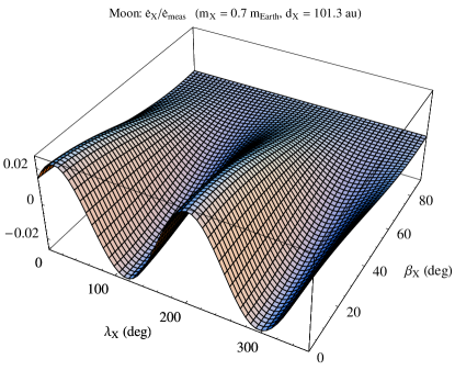
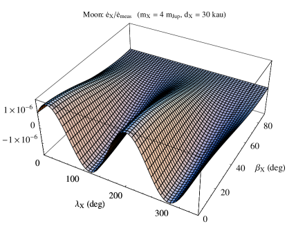
Figure 1: Long-term variation of the lunar eccentricity, normalized to eq. (1), induced by a trans-Plutonian, pointlike object X as a function of its ecliptic latitude $\beta_{\rm X}$ and longitude $\lambda_{\rm X}$. The node $\Omega$ and the perigee $\omega$ of the Moon were kept fixed to the J2000.0 values quoted in Table 1. The scenarios for the perturbing body X are those by Lykawka & Mukai (2008) (left panel), and by Matese & Whitmire (2011) (right panel).

It can be noticed that the physical and orbital features of X postulated by such two recent theoretical models would induce long-term variations of the lunar eccentricity much smaller than eq. (1). Conversely, it turns out that a tidal parameter as large as

$$\mathcal{K}_{\rm X}=4.46\times 10^{-24}\ {\rm s^{-2}}$$ (40)

would yield the result of eq. (1). Actually, eq. (40) is totally unacceptable since it corresponds to distances of X as absurdly small as $d_{\rm X}=30$ au for a terrestrial body, and $d_{\rm X}=200$ au for a Jovian mass (Iorio, 2011).

We must conclude that not even the hypothesis of Planet X is a viable one to explain the anomalous increase of the lunar eccentricity of eq. (1).

4 Summary and conclusions

In this paper we dealt with the anomalous increase of the eccentricity $e$ of the orbit of the Moon recently reported from an analysis of a multidecadal record of LLR data points.

We looked for possible explanations in terms of unmodeled dynamical features of motion within either the standard Newtonian/Einsteinian paradigm or several long-range models of modified gravity. As a general rule, we, first, noticed that it would be misleading to simply find the right order of magnitude for the extra-acceleration due to this or that candidate effect. Indeed, it is mandatory to explicitly check if a potentially viable candidate does actually induce a non-vanishing averaged variation of the eccentricity. This holds, in principle, for the search of an explanation of any other possible anomalous effect. Quite generally, it turned out that any time-independent and spherically symmetric perturbation does not affect the eccentricity with long-term changes.

Thus, most of the long-range modified models of gravity proposed in more or less recent times for other scopes are automatically ruled out. The present-day limits on the magnitude of a terrestrial Rindler-type perturbing acceleration are of the right order of magnitude, but it does not secularly affect $e$. As time-dependent candidates capable to cause secular shifts of $e$, we considered the possible variation of the Earth’s gravitational parameter $\mu$ both because of a temporal variation of the Newtonian constant of gravitation $G$ and of its mass itself due to a steady mass accretion of non-annihilating Dark Matter. In both cases, the resulting time variations of $e$ are too small by several orders of magnitude.

Moving to standard general relativity, we found that the gravitomagnetic Lense-Thirring lunar acceleration due to the Earth’s angular momentum, not modeled in the data analysis, has the right order of magnitude, but it, actually, does not induce secular variations of $e$. The same holds also for other general relativistic spin-dependent effects. Conversely, $e$ undergoes long-term changes caused by the general relativistic first-order effects due to the Earth’s oblateness, but they are far too small. The second-order post-Newtonian part of the gravitational field does not affect the eccentricity.

Within the Newtonian framework, we considered the action of an almost circular massive ring modeling the Edgeworth-Kuiper belt of Trans-Neptunian Objects, but it does not induce secular variations of $e$. In principle, a viable candidate would be a putative trans-Plutonian massive object (PlanetX/Nemesis/Tyche), recently revamped to accommodate certain features of the architecture of the Kuiper belt and of the distribution of the comets in the Oort cloud, since it would cause a non-vanishing long-term variation of the eccentricity. Actually, the values for its mass and distance needed to explain the empirically determined increase of the lunar eccentricity would be highly unrealistic and in contrast with the most recent viable theoretical scenarios for the existence of such a body. For example, a terrestrial-sized body should be located at just 30 au, while an object with the mass of Jupiter should be at 200 au.

Thus, in conclusion, the issue of finding a satisfactorily explanation of the observed orbital anomaly of the Moon still remains open. Our analysis should have effectively restricted the field of possible explanations, indirectly pointing towards either non-gravitational, mundane effects or some artifacts in the data processing. Further data analyses, hopefully performed by independent teams, should help in shedding further light on such an astrometric anomaly.

References

- Adelberger et al. (2003) Adelberger E.G., Heckel B.R., Nelson A.E., 2003, Ann. Rev. Nucl. Part. Sci., 53, 77
- Adkins & McDonnell (2007) Adkins G. S., McDonnell J., 2007, Phys. Rev. D., 75, 082001
- Adkins et al. (2007) Adkins G. S., McDonnell J., Fell R. N., 2007, Phys. Rev. D., 75, 064011
- Adler (2008) Adler S. L., 2008, J. of Physics A: Mathematical and Theoretical, 41, 412002
- Allemandi et al. (2005) Allemandi G., Francaviglia M., Ruggiero M. L., Tartaglia A., 2005, Gen. Relativ. Gravit., 37, 1891
- Anderson & Nieto (2010) Anderson J. D., Nieto M. M., 2010, Astrometric solar-system anomalies. In: Klioner S.A., Seidelmann P.K., Soffel M.H., (eds.) Relativity in Fundamental Astronomy: Dynamics, Reference Frames, and Data Analysis, Proceedings IAU Symposium No. 261, Cambridge University Press, Cambridge, 2010, pp. 189-197
- Apostolopoulos & Tetradis (2006) Apostolopoulos P. S., Tetradis N., 2006, Phys. Rev. D, 74, 064021
- Bertolami & Páramos (2005) Bertolami O., Páramos J., 2005, Phys. Rev. D, 71, 023521
- Bertolami et al. (2007) Bertolami O., Böhmer C. G., Harko T., Lobo F. S. N., 2007, Phys. Rev. D, 75, 104016
- Bertolami & Santos (2009) Bertolami O., Santos N. M. C., 2009, Phys. Rev. D, 79, 127702
- Bertotti et al. (2003) Bertotti B., Farinella P., Vokrouhlický D., 2003, Physics of the Solar System, Kluwer Academic Press, Dordrecht
- Blinnikov & Khlopov (1983) Blinnikov S. I., Khlopov M. Yu., 1983, Sov. Astron., 27, 371.
- Brosche & Schuh (1998) Brosche P., Schuh H., 1998, Surv. Geophys., 19, 417
- Brownstein & Moffat (2006) Brownstein J. R., Moffat J. W., 2006, Class. Quantum Grav., 23, 3427
- Burgess & Cloutier (1988) Burgess C.P., Cloutier J., 1988, Phys. Rev. D, 38, 2944
- Capozziello (2007) Capozziello S., 2007, Int. J. Geom. Meth. Mod. Phys., 4, 53
- Capozziello et al. (2001) Capozziello S., De Martino S., De Siena S., Illuminati F., 2001, Mod. Phys. Lett. A, 16, 693
- Capozziello & Lambiase (2003) Capozziello S., Lambiase G., 2003, Int. J. Mod. Phys. D, 12, 843
- Capozziello et al. (2006) Capozziello S., Cardone V. F., Francaviglia M., 2006, Gen. Relativ. Gravit., 38, 711
- Capozziello & Francaviglia (2008) Capozziello S., Francaviglia M., 2008, Gen. Relativ. Gravit., 40, 357
- Damour & Schäfer (1988) Damour T., Schäfer G., 1988, Nuovo Cimento B, 101, 127
- de Felice & Tsujikawa (2010) de Felice A., Tsujikawa S., 2010, Living Rev. Rel., 13, 3
- Dirac (1937) Dirac P. A. M., 1937, Nature, 139, 323
- Dvali et al. (2000) Dvali G., Gabadadze G., Porrati M., 2000, Phys. Lett. B, 485, 208
- Dvali et al. (2003) Dvali G., Gruzinov A., Zaldarriaga M., 2003, Phys. Rev. D, 68, 024012
- Edgeworth (1943) Edgeworth K. E., 1943, J. Brit. Astron. Assoc., 53, 181
- Fabrina et al. (2011) Farina C., Kort-Kamp W. J. M., Mauro Filho S., Shapiro I. L., 2011, arXiv:1101.5611
- Fernández (2011) Fernández J.A., 2011, ApJ, 726, 33
- Fienga et al. (2008) Fienga A., Manche H., Laskar J., Gastineau M., 2008, Astron. Astrophys., 477, 315
- Folkner et al. (2008) Folkner W. M., Williams J. G., Boggs D. H., 2008, The Planetary and Lunar Ephemeris DE 421, JPL IOM 343R-08-003
- Foot (2004) Foot R., 2004, Int. J. Mod. Phys. D, 13, 2161
- Grumiller (2010) Grumiller D., 2010, Phys. Rev. Lett., 105, 211303
- Gruzinov (2005) Gruzinov A., 2005, New Astron., 10, 311
- Heimberger et al. (1990) Heimberger J., Soffel M., Ruder H., 1990, Celest. Mech. Dyn. Astron., 47, 205
- Hogg et al. (1991) Hogg D., Quinlan G., Tremaine S., 1991, AJ, 101, 2274
- Hořava (2009a) Hořava P., 2009a, Phys. Rev. D, 79, 84008
- Hořava (2009b) Hořava P., 2009b, Phys. Rev. Lett. 102, 161301
- Iorio (2007) Iorio L., 2007, Found. Phys., 73, 897
- Iorio (2010a) Iorio L., 2010a, arXiv:1012.0226
- Iorio (2010b) Iorio L., 2010b, Schol. Res. Exch., 2010, 261249
- Iorio (2010c) Iorio L., 2010c, J. Cosmol. Astropart. Phys., 05, 018
- Iorio (2010d) Iorio L., 2010d, arXiv:1012.5622
- Iorio (2011) Iorio L., 2011, arXiv:1101.2634
- Iorio & Ruggiero (2009) Iorio L., Ruggiero M. L., 2009, J. Cosmol. Astropart. Phys., 03, 024
- Iorio & Ruggiero (2010) Iorio L., Ruggiero M. L., 2010, Int. J. Mod. Phys. A., 25, 5399
- Jaekel & Reynaud (2005a) Jaekel M.-T., Reynaud S., 2005a, Mod. Phys. Lett. A, 20, 1047
- Jaekel & Reynaud (2005b) Jaekel M.-T., Reynaud S., 2005b, Class. Quantum Grav., 22, 2135
- Jaekel & Reynaud (2006a) Jaekel M.-T., Reynaud S., 2006a, Class. Quantum Grav., 23, 777
- Jaekel & Reynaud (2006b) Jaekel M.-T., Reynaud S., 2006b, Class. Quantum Grav., 23, 7561
- Kehagias & Sfetsos (2009) Kehagias A., Sfetsos K., 2009, Phys. Lett. B, 678, 123
- Kerr et al. (2003) Kerr A. W., Hauck J. C., Mashhoon B., 2003, Class. Quantum Grav., 20, 2727
- Khlopov et al. (1991) Khlopov M. Yu., Beslin G. M., Bochkarev N. G., Pustil’nik L. A., Pustil’nik S. A., 1991, Sov. Astron., 35, 21
- Khlopov (1999) Khlopov M. Yu., 1999, Cosmoparticle physics, World Scientific, Singapore
- Krasinsky et al. (2002) Krasinky G. A., Pitjeva E. V., Vasilyev M. V., Yagudina E. I., 2002, Icarus, 158, 98
- Khriplovich & Shepelyansky (2009) Khriplovich I. B., Shepelyansky D. L., 2009, Int. J. Mod. Phys. D, 18, 1903
- Kuiper (1951) Kuiper G. P., 1951, in Hynek J. A., ed., Proc. Topical Symp. Commemorating the 50th Anniversary of the Yerkes Observatory and Half a Century of Progress in Astrophysics. McGraw-Hill, New York, p. 357
- Lense & Thirring (1918) Lense J., Thirring H., 1918, Phys. Z., 19, 156
- Lykawka & Mukai (2008) Lykawka P.S., Mukai T., 2008, AJ, 135, 1161
- Matese & Whitmire (2011) Matese J.J., Whitmire D.P., 2011, Icarus, 211, 926
- McCarthy & Petit (2004) McCarthy D.D., Petit G., 2004, IERS Technical Note No. 32. IERS Conventions (2003). 12. Frankfurt am Main: Verlag des Bundesamtes für Kartographie und Geodäsie
- Melott & Bambach (2010) Melott A.L., Bambach R.K., 2010, MNRAS, 407, L99
- Milne (1935) Milne E. A., 1935, Relativity, Gravity and World Structure. Oxford: Clarendon Press
- Moffat (2006) Moffat J. W., 2006, J. Cosmol. Astropart. Phys., 0603, 004
- Müller & Biskupek (2007) Müller J., Biskupek L., 2007, Class. Quantum Gravit., 24, 4533
- Müller et al. (2007) Müller J., Williams J. G., Turyshev S. G., Shelus P. J., 2007, Potential Capabilities of Lunar Laser Ranging for Geodesy and Relativity. In: Tregoning P., Rizos C. (eds.) Dynamic Planet. International Association of Geodesy Symposia Volume 130, Part IX, Springer, Berlin, pp. 903-909
- Müller et al. (2008) Müller J., Williams J. G., Turyshev S. G., 2008, Lunar Laser Ranging Contributions to Relativity and Geodesy. In: Dittus H., Lämmerzahl C., Turyshev S. G. (eds.) Lasers, Clocks and Drag-Free Control. Astrophysics and Space Science Library Volume 349, Springer, Berlin, pp. 457-472
- Müller et al. (2009) Müller J., Biskupek L., Oberst J., Schreiber U., 2009, Contribution of Lunar Laser Ranging to Realise Geodetic Reference Systems. In: Drewes H. (ed.) Geodetic Reference Frames. International Association of Geodesy Symposia Volume 134, Part 2, Springer, Berlin, pp. 55-59,
- Murray & Dermott (1999) Murray C. D., Dermott S. F., 1999, Solar System Dynamics, Cambridge University Press, Cambridge
- Murray & Correia (2010) Murray C.D., Correia A.C.M., 2010, Keplerian Orbits and Dynamics. In: Seager S. (ed.), Exoplanets, University of Arizona Press, Tucson, pp. 15-23
- Navarro & van Acoleyen (2005) Navarro I., van Acoleyen K., 2005, Phys. Lett. B, 622, 1
- Navarro & van Acoleyen (2006a) Navarro I., van Acoleyen K., 2006a, J. Cosmol. Astropart. Phys., 008, 003
- Navarro & van Acoleyen (2006b) Navarro I., van Acoleyen K., 2006b, J. Cosmol. Astropart. Phys., 006, 009
- Nojiri & Odintsov (2007) Nojiri S., Odintsov S. D., 2007, Int. J. Geom. Meth. Mod. Phys., 4, 115
- Nordtvedt (1996) Nordtvedt K., 1996, Class. Quantum Gravit., 13, A11
- Pitjeva (2010) Pitjeva E.V, 2010, EPM ephemerides and relativity. In: Klioner S.A., Seidelmann P.K., Soffel M.H., (eds.) Relativity in Fundamental Astronomy: Dynamics, Reference Frames, and Data Analysis, Proceedings IAU Symposium No. 261, Cambridge University Press, Cambridge, 2010, pp. 170-178.
- Reynaud & Jaekel (2005) Reynaud S., Jaekel M.-Th., 2005, I. J. Mod. Phys. A, 20, 2294
- Roncoli (2005) Roncoli R. B., 2005, Lunar Constants and Models Document, JPL D-32296, Jet Propulsion Laboratory, California Institute of Technology
- Ruggiero (2010) Ruggiero M. L., 2010, arXiv:1010.2114
- Ruggiero & Iorio (2010) Ruggiero M. L., Iorio L., 2010, Gen. Relativ. Gravit., 42, 2393
- Sanders (2006) Sanders R. H., 2006, Mon. Not. R. Astron. Soc., 370, 1519
- Schäfer & Wex (1993) Schäfer G., Wex N., 1993, Phys. Lett. A, 174, 196
- Seidelmann (1992) Seidelmann P. K. (ed.), 1992, Explanatory Supplement to the Astronomical Almanac, University Science Books, Mill Valley, CA,
- Soffel et al. (1988) Soffel M., Wirrer R., Schastok J., Ruder H., Schneider M., 1988, Celest. Mech. Dyn. Astron., 42, 81
- Soffel (1989) Soffel M.H., 1989, Relativity in Astrometry, Celestial Mechanics and Geodesy, Springer Verlag, Berlin
- Sotiriou & Faraoni (2010) Sotiriou T., Faraoni V., 2010, Rev. Mod. Phys., 82, 451
- Wex (1995) Wex N., 1995, Class. Quantum Gravit., 12, 983
- Williams et al. (2001) Williams J. G., Boggs D. H., Yoder C. F., Ratcliff J. T., Dickey J. O., 2001, J. Geophys. Res., 106, 27933
- Williams & Dickey (2003) Williams J. G., Dickey J. O., 2003, Lunar Geophysics, Geodesy, and Dynamics. In: Noomen R., Klosko S., Noll C., Pearlman M. (eds.) Proceedings of the 13th International Workshop on Laser Ranging, NASA/CP-2003-212248, pp. 75-86. http://cddis.nasa.gov/lw13/docs/papers/sciwilliams1m.pdf
- Williams et al. (2007) Williams J. G., Turyshev S. G., Boggs D. H., 2007, Phys. Rev. Lett., 98, 059002
- Williams et al. (2008) Williams J. G., Boggs D. H., Folkner W. M., 2008, DE421 Lunar Orbit, Physical Librations, and Surface Coordinates, JPL IOM 335-JW,DB,WF-20080314-001
- Williams & Boggs (2009) Williams J. G., Boggs D. H., 2009, Lunar Core and Mantle. What Does LLR See? In: Schilliak S. (eds.) Proceedings of the 16th International Workshop on Laser Ranging, pp. 101-120. http://cddis.gsfc.nasa.gov/lw16/docs/papers/sci1Williamsp.pdf
- Xu & Siegel (2008) Xu X., Siegel E. R., 2008, arXiv:0806.3767