Force-extension curves of bacterial flagella

Abstract

Bacterial flagella assume different helical shapes during the tumbling phase of a bacterium but also in response to varying environmental conditions. Force-extension measurements by Darnton and Berg explicitly demonstrate a transformation from the coiled to the normal helical state [N. C. Darnton and H. C. Berg, Biophys. J. 92, 2230 (2007)]. We here develop an elastic model for the flagellum based on Kirchhoff’s theory of an elastic rod that describes such a polymorphic transformation and use resistive force theory to couple the flagellum to the aqueous environment. We present Brownian dynamics simulations that quantitatively reproduce the force-extension curves and study how the ratio $\Gamma$ of torsional to bending rigidity and the extensional rate influence the response of the flagellum. An upper bound for $\Gamma$ is given. Using clamped flagella, we show in an adiabatic approximation that the mean extension, where a local coiled-to-normal transition occurs first, depends on the logarithm of the extensional rate.

1 Introduction

Many types of bacteria, such as Escherichia coli and Salmonella typhimurium, propel themselves forward by rotating a bundle of elastic filaments with helical shape. Each of these flagella, as they are called, is driven by a rotary motor. When the sense of rotation of one motor is reversed, the attached flagellum leaves the bundle and undergoes a sequence of different helical configurations characterized by their pitch, radius and helicity. During the flagellar polymorphism, the bacterium tumbles and then continues swimming in a different direction, when the flagellum assumes its original form and returns into the bundle. Whenever the bacterium senses a positive food gradient, it prolongs the swimming phase and thereby increases the food uptake Berg04 . In recent years, bacteria and their flagella have also been used in studies relevant to microfluidics to transport colloids Zhang2009 ; Behkam2007 and pump fluids Kim2008 but also to create new liquid-crystalline phases of screw like objects Barry2006 . An understanding of the bacterial tumbling motion and the applications of bacterial flagella in nanotechnology and microfluidics requires a sufficiently simple elastic model that includes the flagellar polymorphism. This article aims to provide such a model.

The bacterial flagellum consists of three parts. The rotary motor is embedded in the cell membrane and transmits its motor torque to the long helical filament with the help of the short and very flexible proximal hook. The filament of E.coli bacteria is up to 10 $\mathrm{\SIUnitSymbolMicro}\mathrm{m}$ long and is about 0.02 $\mathrm{\SIUnitSymbolMicro}\mathrm{m}$ in diameter. It is relatively stiff but can switch between distinct polymorphic forms. The filament assumes these forms in response to external perturbations such as changes in pH value, salinity, and temperature of the surrounding fluid Kamiya76 ; Kamiya77 ; Hasegawa82 , the addition of alcohols Hotani80 or sugars Seville93 , and by applying external forces or torques to the filament Macnab77 ; Hotani82 ; Darnton07a ; Darnton07 .

The helical filament is a cylinder formed by 11 protofilaments each of which consists of a stack of protein monomers called flagellin. These monomers assume two conformations (L and R) that mainly differ in length. Each protofilament only contains one type of monomer and therefore L- and R-state protofilaments have different lengths. Mixing them in the flagellar filament produces bending which together with an intrinsic twist of the filament gives a helical configuration. In total two straight and 10 helical polymorphic states are possible since protofilaments of one type cluster (see Fig. 1). Most of them were observed experimentally Hasegawa1998 . This is the picture Asakura Asakura70 and later Calladine Calladine75 , with a more detailed geometric model, developed to explain the flagellar polymorphism. The molecular structure for the flagellar filament was confirmed recently Yamashita98 ; Yonekura03 and several extensions of Calladine’s model exist Hasegawa1998 ; Srigiriraju2005 ; Srigiriraju2006 ; Friedrich2006 ; Speier09 .

Figure 1: Twelve polymorphic states of the bacterial flagellum with curvature $\kappa=\kappa_{\mathtt{max}}\sin(\pi n_{R}/11)$ and torsion $\tau=\tau_{L}+(\tau_{R}-\tau_{L})n_{R}/11$ after Calladine Calladine75 , where $n_{R}$ is the number of protofilaments in the R state. The quantities $\kappa_{\mathtt{max}}\approx 2.4\mathrm{/}\mathrm{\SIUnitSymbolMicro}\mathrm{m}$, $\tau_{L}\approx-5.2\mathrm{/}\mathrm{\SIUnitSymbolMicro}\mathrm{m}$, and $\tau_{R}\approx 11.8\mathrm{/}\mathrm{\SIUnitSymbolMicro}\mathrm{m}$ are fit parameters.

This article is mainly motivated by recent experiments of Darnton and Berg Darnton07 . With the help of an optical tweezer set up they pulled the two ends of the flagellar filament apart with a constant velocity and induced a transition between two polymorphic configurations. They then reversed the velocity to compress the flagellum in order to return it to the initial configuration. Darnton and Berg recorded force-extension curves mainly for the transformation from the coiled to the normal configuration. The transformation starts locally at one end of the flagellum and then proceeds in discrete steps along the flagellum. Signatures of the steps are clearly visible in the force-extension curves.

Calculating the force-extension curves on the basis of coarse-grained molecular dynamics simulations is not possible since simulation times are far below the experimentally relevant time scale of one second arkh:06 . Modeling the polymorphism of a bacterial flagellum on a mesoscopic level is more appropriate. Goldstein et al. extended Kirchhoff’s classic theory of an elastic rod by introducing a double-well potential for the spontaneous torsion to describe the transition between two helical states Goldstein2000 ; Coombs2002 . Wada and Netz also described the helical filament by Kirchhoff’s rod theory but attached a spin variable along the filament in order to distinguish locally between the two helical states Wada2008 . They then performed hybrid Brownian-dynamics Monte-Carlo simulations to numerically calculate force-extension curves of bacterial flagella.

In this article we present Brownian-dynamics simulations of the force-extension curves based on a model that is less time-consuming than the approach of Ref. Wada2008 but that is completely equivalent as we demonstrate in an appendix. We furthermore concentrate on different aspects of the force-extension curves, namely how they depend on the ratio of torsional and bending rigidities $\Gamma$ and on the velocity or extensional rate with which the flagellum is pulled apart. We also give an upper bound for $\Gamma$ which is partially in contrast to experimental results. The mean extension, at which a coiled-to-normal transition first occurs locally, is a function of the extension rate. We demonstrate how this extension can be inferred from equilibrium properties of a clamped helical filament. Our modeling is in the spirit of Refs. Goldstein2000 ; Coombs2002 . However, we show that a conventional double-well potential cannot reproduce the experimentally observed force extension curves. We therefore developed an alternative model, where we just “glue” the harmonic elastic energies of the two helical states together. We perform our simulations with realistic parameter values and can directly compare our results to experiments.

The article is organized as follows. In Section 2 we present our extension of Kirchhoff’s elastic rod theory to include the polymorphism of helical filaments, explain how we perform the Brownian dynamics simulations, and present analytic results for a uniformly stretched conventional helical filament. Section 3 discusses the results for the simulated force-extension curves and addresses the clamped filament. We close with a summary and conclusions in Section 4.

2 Continuum model for the bacterial flagellum

2.1 Classic theory of an elastic rod

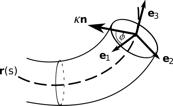
Figure 2: The conformation of a slender elastic rod is described by the space curve $\boldsymbol{r}(s)$ of its center line and the material frame $\{\boldsymbol{e}_{1},\boldsymbol{e}_{2},\boldsymbol{e}_{3}\}$. The vector $\kappa\boldsymbol{n}=\partial_{s}\boldsymbol{e}_{3}$ describes the local curvature of $\boldsymbol{r}(s)$.

The conformation of a slender rod with contour length $L$ is described by the space curve of its center line $\boldsymbol{r}(s)$, parametrized by the arc length $s$, and a material frame of three orthogonal unit vectors $\{\boldsymbol{e}_{1},\boldsymbol{e}_{2},\boldsymbol{e}_{3}\}$, attached to each point on the center line. The vector $\boldsymbol{e}_{3}$ points along the tangent of $\boldsymbol{r}(s)$ and $\boldsymbol{e}_{1},\boldsymbol{e}_{2}$ typically correspond to the principal axes of the inertia tensor of the cross section as indicated in Fig. 2. Since the $\boldsymbol{e}_{i}$ are unit vectors, the transport of the material frame along the center line is described by the generalized Frenet-Serret equations

$$\partial_{s}\boldsymbol{e}_{i}=\boldsymbol{\Omega}\times\boldsymbol{e}_{i},$$ (1)

where $\partial_{s}$ means derivative with respect to $s$. So the conformation of an elastic rod or filament is completely characterized by the angular strain vector $\boldsymbol{\Omega}=(\Omega_{1},\Omega_{2},\Omega_{3})$. Alternatively, one uses the Frenet frame consisting of the tangent vector $\boldsymbol{t}=\boldsymbol{e}_{3}$, the curvature vector $\kappa\boldsymbol{n}=\partial_{s}\boldsymbol{t}$, and the binormal $\boldsymbol{b}=\boldsymbol{t}\times\boldsymbol{n}$. The Frenet frame transforms into the material frame when it is rotated about $\boldsymbol{t}=\boldsymbol{e}_{3}$ by the twist angle $\phi$, as indicated in Fig. 2. This relates the vector $\boldsymbol{\Omega}$ to the curvature $\kappa$ and torsion $\tau$ of the filament:

$$\Omega_{1} =\kappa\sin\phi, \Omega_{2} =\kappa\cos\phi, \Omega_{3} =\tau+\partial_{s}\phi,$$ (2)

where the components $\Omega_{i}$ are given with respect to the local material frame.

Kirchhoff’s theory expands the elastic free energy $\mathcal{F}$ of a deformed elastic rod up to second order in the angular strain $\boldsymbol{\Omega}$,

$${\mathcal{F}}= \int_{0}^{L}f_{\mathtt{cl}}(\boldsymbol{\Omega},\boldsymbol{\Omega}_{0})\mathrm{d}s$$ (3)

$$f_{\mathtt{cl}}(\boldsymbol{\Omega},\boldsymbol{\Omega}_{0}) =\frac{A}{2}(\Omega_{1})^{2}+\frac{A}{2}(\Omega_{2}-\kappa_{0})^{2}+\frac{C}{2}(\Omega_{3}-\tau_{0})^{2},$$ (4)

where we also introduced a spontaneous curvature $\kappa_{0}$ and torsion $\tau_{0}$ within $\boldsymbol{\Omega}_{0}=(0,\kappa_{0},\tau_{0})$, and $A$ is the bending rigidity and $C$ the torsional rigidity Love1944 ; Landau1986 . Since the bacterial flagellum has a circular cross section, we can choose for the material frame the Frenet frame in the undeformed ground state, meaning $\phi=0$, and thereby restrict the spontaneous curvature $\kappa_{0}$ to $\Omega_{2}$. If $\kappa_{0}$ and $\tau_{0}$ are constant along the filament, it has a helical shape with pitch $p=2\pi\tau_{0}/(\kappa_{0}^{2}+\tau_{0}^{2})$ and radius $r=\kappa_{0}/(\kappa_{0}^{2}+\tau_{0}^{2})$. Note that although free energy (3) is formulated in the spirit of linear elasticity theory, it becomes highly nonlinear when expressed in terms of the space curve $\boldsymbol{r}(s)$ and twist angle $\phi$.

2.2 Extended Kirchhoff rod theory

In order to describe the transition of the bacterial flagellum between two polymorphic configurations, the Kirchhoff rod theory has to be extended to include two local ground states characterized by $\boldsymbol{\Omega}_{i}=(0,\kappa_{i},\tau_{i})$ ($i=1,2$). We first tried to generalize the approach of Goldstein et al., who used a typical double well potential for the twist density $\Omega_{3}$ Goldstein2000 ; Coombs2002 (see Appendix A) . However, the force-extension curves calculated with this extended free energy by numerical simulations did not reproduce the experimental curves as indicated in Appendix A.

We, therefore, developed a different model. To each of the two relevant polymorphic forms of the flagellum we assign the elastic free energy (3) of Kirchoff’s rod theory and introduce a difference $\delta$ of the two energy densities in the ground states. Since the free energy of a system always assumes a minimum, we locally assign to the bacterial flagellum with angular strain $\boldsymbol{\Omega}$ the minimum $f_{\mathtt{poly}}(\boldsymbol{\Omega},\boldsymbol{\Omega}_{1},\boldsymbol{\Omega}_{2})$ of the free energy densities of the two polymorphic configurations:

$$f_{\mathtt{poly}}(\boldsymbol{\Omega},\boldsymbol{\Omega}_{1},\boldsymbol{\Omega}_{2})=\min\big{(}f_{\mathtt{cl}}(\boldsymbol{\Omega},\boldsymbol{\Omega}_{1}),f_{\mathtt{cl}}(\boldsymbol{\Omega},\boldsymbol{\Omega}_{2})+\delta\big{)},$$ (5)

where $f_{\mathtt{cl}}$ is the elastic free energy density of Eq. (4). The resulting density $f_{\mathtt{poly}}(\boldsymbol{\Omega},\boldsymbol{\Omega}_{1},\boldsymbol{\Omega}_{2})$ is plotted in Fig. 3 as a function of curvature $\kappa$ and torsion $\tau$ using Eq. (2) and assuming $\phi=0$.

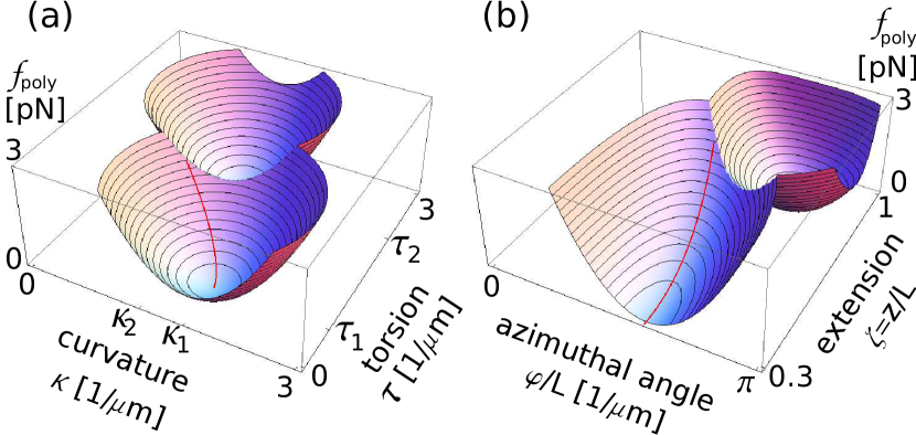
Figure 3: (a) Free energy density $f_{\mathtt{poly}}$ from Eq. (5) as a function of curvature $\kappa$ and torsion $\tau$ using $\boldsymbol{\Omega}=(0,\kappa,\tau)$. (b) Free energy density $f_{\mathtt{poly}}$ as a function of height $z$ and azimuthal angle per unit length $\varphi/L$ of a uniformly stretched helical filament (see Section 2.5). The red lines indicate the path of the helical filament in the energy landscape during stretching.

Wada and Netz formulated an alternative, statistical model to access the polymorphism of the bacterial flagellum Wada2008 which they described as a bead-spring chain. To each bead they assigned the Kirchoff free energy (4) and an Ising spin to distinguish locally between the two polymorphic forms of the flagellum. The Ising spin Hamiltonian then favored the same polymorphic state for adjacent beads. By integrating out the spin degree of freedom, they derived an effective free energy density which we summarize in Appendix B. In experiments, where a thermally induced transition from the normal to the semi-coiled configuration was studied, most flagella assumed a pure polymorphic form of either the normal or semi-coiled state Hasegawa82 suggesting that the energy cost for forming a domain wall between the two helical states is much larger than thermal energy. Using this observation, we demonstrate in Appendix B that the free energy density of Wada and Netz simplifies to our elastic free energy (5).

Note that our ansatz can easily be extended to describe more than two of the polymorphic states of bacterial flagella. In particular, this will be necessary for understanding the sequence of polymorphic transitions during the tumbling phase of E. coli.

The elastic free energy density $f_{\mathtt{poly}}$ of Eq. (5) admits that two domains of different polymorphic states are separated from each other by a sharp domain wall with zero width. To realize a more realistic, smoother transition between two domains, we have to introduce a free energy density of the form Goldstein2000

$$f_{\mathtt{bi}}(\partial_{s}\boldsymbol{\Omega})=\frac{\gamma}{2}\left(\partial_{s}\boldsymbol{\Omega}\right)^{2},$$ (6)

where $\gamma^{1/2}$ is proportional to the width of the domain wall. With a properly adjusted $\gamma$, experimental observations of the domain wall could be described quantitatively Goldstein2000 ; Hotani82 . Furthermore, our simulations demonstrated that the helical filament contains several domains instead of just two when $\gamma$ is chosen too small or even equal to zero.

Instead of implementing a constraint for the filament to be inextensible, we introduce a stretching free energy density $f_{\mathtt{st}}=K\left(\partial_{s}\boldsymbol{r}\right)^{2}/2$. We choose the spring constant $K$ such that the changes in the filament length are below 1.5 %. So the filament is inextensible to a good approximation.

Collecting all the contributions, the total elastic free energy ${\mathcal{F}}=\int_{0}^{L}f\mathrm{d}s$, which we will use in the following for modeling the bacterial flagellum, is based on the density

$$f= f_{\mathtt{poly}}(\boldsymbol{\Omega},\boldsymbol{\Omega}_{1},\boldsymbol{\Omega}_{2})+f_{\mathtt{bi}}(\partial_{s}\boldsymbol{\Omega})+f_{\mathtt{st}}(\partial_{s}\boldsymbol{r}).$$ (7)

Since $f$ ultimately depends on the centerline $\boldsymbol{r}(s)$ and the twist angle $\phi(s)$, the total free energy is a functional ${\mathcal{F}}[\boldsymbol{r}(s),\phi(s)]$ in $\boldsymbol{r}(s)$ and $\phi(s)$.

2.3 Dynamics of a Helical Rod

We formulate Langevin equations for the location $\boldsymbol{r}(s)$ and intrinsic twist $\phi(s)$ of the helical filament. At low Reynolds number the sum of elastic force per unit length, $\boldsymbol{f}_{\mathtt{el}}=-\delta\cal F/\delta\boldsymbol{r}$, and thermal force $\boldsymbol{f}_{\mathtt{th}}$ is balanced by viscous drag. The same applies to the elastic torque per unit length, $m_{\mathtt{el}}=-\delta\cal F/\delta\phi$ and thermal torque $m_{\mathtt{th}}$. Using resistive force theory Childress1981 that employs local friction coefficients $\gamma_{\parallel},\gamma_{\perp}$ and $\gamma_{R}$ (see Appendix C), we formulate the Langevin equations

$$\left[\gamma_{\parallel}\boldsymbol{t}\otimes\boldsymbol{t}+\gamma_{\perp}(\boldsymbol{\sf 1}-\boldsymbol{t}\otimes\boldsymbol{t})\right]\boldsymbol{v}= \boldsymbol{f}_{\mathtt{el}}+\boldsymbol{f}_{\mathtt{th}}$$ (8)

$$\gamma_{R}\omega= m_{\mathtt{el}}+m_{\mathtt{th}}.$$ (9)

Here $\boldsymbol{v}=\partial_{t}\boldsymbol{r}$ is the translational velocity, $\omega=\partial_{t}\phi$ the angular velocity about the local tangent vector $\boldsymbol{t}=\boldsymbol{e}_{3}$, and $\otimes$ means tensorial product. The anisotropic friction tensor acting on $\boldsymbol{v}$ in Eq. (8) couples rotation about the helical axis to translation and thereby creates the thrust force that pushes the bacterium forward Purcell1977 . The friction coefficients per unit length were calculated by Lighthill from slender-body theory taking into account the helical geometry of the rod Lighthill1976 . The coefficients are summarized in Appendix C. In experiments one finds reasonable agreement with this approach Chattopadhyay2006 ; Chattopadhyay2009 . The thermal force $\boldsymbol{f}_{\mathtt{th}}$ and torque $m_{\mathtt{th}}$ are Gaussian stochastic variables with zero mean, $\langle\boldsymbol{f}_{\mathtt{th}}\rangle=\boldsymbol{0}$ and $\langle m_{\mathtt{th}}\rangle=0$. Their variances obey the fluctuation-dissipation theorem and therefore read

$$\left\langle\boldsymbol{f}_{\mathtt{th}}(t,s)\otimes\boldsymbol{f}_{\mathtt{th}}(t^{\prime},s^{\prime})\right\rangle =2k_{B}T\delta(t-t^{\prime})\delta(s-s^{\prime})$$ (10)

$$\times\left[\gamma_{\parallel}^{-1}\boldsymbol{t}\otimes\boldsymbol{t}+\gamma_{\perp}^{-1}(\boldsymbol{\sf 1}-\boldsymbol{t}\otimes\boldsymbol{t})\right],$$

$$\left\langle m_{\mathtt{th}}(t,s)m_{\mathtt{th}}(t^{\prime},s^{\prime})\right\rangle =2k_{B}T\delta(t-t^{\prime})\delta(s-s^{\prime})\gamma_{R}^{-1},$$ (11)

$$\left\langle m_{\mathtt{th}}(t,s)\boldsymbol{f}_{\mathtt{th}}(t^{\prime},s^{\prime})\right\rangle =\boldsymbol{0}.$$ (12)

2.4 Details of Simulations

In our simulations we used a technique developed by Reichert Reichert2006 similar to the one of Chirico and Langowski Chirico1994 and also employed by Wada and Netz in simulations of helical nano springs etc. Wada2007a ; Wada2007 . We discretize the centerline $\boldsymbol{r}(s)$ of the filament by introducing $N+1$ beads at locations $\boldsymbol{r}^{i}=\boldsymbol{r}(s=i\cdot h)$ and with nearest-neighbor distance $h$. To every bead we attach the material frame, i.e., a right-handed tripod of orthonormal vectors $\{\boldsymbol{e}^{i}_{1},\boldsymbol{e}^{i}_{2},\boldsymbol{e}^{i}_{3}\}$ ($i=0,\dots,N$), where the tangent vector is approximated by

$$\boldsymbol{e}_{i}^{3} =\frac{\boldsymbol{r}_{i}-\boldsymbol{r}_{i-1}}{|\boldsymbol{r}_{i}-\boldsymbol{r}_{i-1}|}.$$ (13)

We split the rotation of the tripod along the filament into two parts. First, we rotate about the bond direction $\boldsymbol{e}_{i}^{3}$ by an angle $\Omega_{i}^{3}h$ corresponding to the intrinsic twist plus torsion. Thereafter, the tripod is rotated such that the bond orientation $\boldsymbol{e}_{3}^{i}$ is transformed into the consecutive direction $\boldsymbol{e}_{3}^{i+1}$, thus describing the curvature of the filament. With this procedure the free energy density $f$ of Eq. (7) is discretized and the functional derivatives of the total free energy, $\boldsymbol{f}_{\mathtt{el}}=-\delta\cal F/\delta\boldsymbol{r}$ and $m_{\mathtt{el}}=-\delta\cal F/\delta\phi$, reduce to conventional derivatives with respect to $\boldsymbol{r}^{i}$ and $\phi^{i}$. We also note that the tangent vector in the friction tensor in Eq. (8) is approximated by $\boldsymbol{t}^{i}=(\boldsymbol{e}_{3}^{i}+\boldsymbol{e}_{3}^{i+1})/|\boldsymbol{e}_{3}^{i}+\boldsymbol{e}_{3}^{i+1}|$.

In the following, we will discuss the influence of the three relevant parameters on the force-extension curves; the ratio $\Gamma=C/A$ of the torsional and bending rigidities (twist-to-bend ratio $\Gamma$), the difference in energy $\delta$ of the two helical ground states under study, and the velocity or extensional rate $v_{p}$ with which the bacterial flagellum is pulled apart. The bending rigidity $A$ together with an appropriate length introduces characteristic values for force and elastic energy. We used $A=3.5\mathrm{p}\mathrm{N}\mathrm{\SIUnitSymbolMicro}\mathrm{m}^{2}$ given in Ref. Darnton07 as a typical value for bacterial flagella. All other parameters are determined by the geometry of the two polymorphic states. Initially, the bacterial flagellum is in the coiled state with spontaneous curvature $\kappa_{1}=1.8\mathrm{/}\mathrm{\SIUnitSymbolMicro}\mathrm{m}$ and torsion $\tau_{1}=0.56\mathrm{/}\mathrm{\SIUnitSymbolMicro}\mathrm{m}$ and then switches into the normal state with $\kappa_{2}=1.3\mathrm{/}\mathrm{\SIUnitSymbolMicro}\mathrm{m}$ and $\tau_{2}=2.1\mathrm{/}\mathrm{\SIUnitSymbolMicro}\mathrm{m}$.

The friction coefficients are calculated with the formulas of Lighthill Lighthill1976 summarized in Appendix C as $\gamma_{\parallel}=1.6\cdot 10^{-3}\mathrm{p}\mathrm{N}\mathrm{s}\mathrm{/}\mathrm{\SIUnitSymbolMicro}\mathrm{m}^{2}$, $\gamma_{\perp}=2.8\cdot 10^{-3}\mathrm{p}\mathrm{N}\mathrm{s}\mathrm{/}\mathrm{\SIUnitSymbolMicro}\mathrm{m}^{2}$, and $\gamma_{R}=0.126\cdot 10^{-3}\mathrm{p}\mathrm{N}\mathrm{s}$ where a filament diameter of around $20\mathrm{n}\mathrm{m}$ was used. The length of the filament is $L=10\mathrm{\SIUnitSymbolMicro}\mathrm{m}$ corresponding to approximately three helical turns in the coiled and four in the normal state. The discretization length between the beads was chosen as $h=0.2\mathrm{\SIUnitSymbolMicro}\mathrm{m}$ and the elastic coefficient in Eq. (6) as $\gamma=0.1\mathrm{p}\mathrm{N}\mathrm{\SIUnitSymbolMicro}\mathrm{m}^{4}$.

2.5 Uniform Deformation

A helical filament of length $L$ much larger than the pitch deforms uniformly aside from inhomogeneities at both ends when a constant external force pulls at it. This means curvature $\kappa$ and torsion $\tau$ are constant along the filament. We orient the helical axis along the $z$ axis of a cylindrical coordinate system $(\rho,\varphi,z)$. The geometry and free energy of the uniformly deformed helix are completely described by its height $z=L\frac{\tau}{\sqrt{\kappa^{2}+\tau^{2}}}$ and the difference in azimuthal angles of both ends of the filament, $\varphi=\varphi(s=L)=L\sqrt{\kappa^{2}+\tau^{2}}$, where we set $\varphi(s=0)=0$. Then, the force and torque acting on a uniformly stretched helix follows from $F=-\partial_{z}\mathcal{F}(z,\varphi)$ and $T=-\partial_{\varphi}\mathcal{F}(z,\varphi)$, respectively. In experiments, the ends of the filament can freely rotate during stretching which means zero torque $T$. This leads to an expression for $\varphi/L$

$$\frac{\varphi}{L} =\frac{\kappa_{0}\cos\alpha+\Gamma\tau_{0}\sin\alpha}{(1+\Gamma)\cos^{2}\alpha}$$ (14)

where we introduced the pitch angle $\alpha$ using the extension

$$\zeta=z/L=\sin\alpha.$$ (15)

Under the condition of zero torque, we then obtain the classic force-extension relation Love1944

$$F(z) =\frac{A(\Gamma\kappa_{0}\cos\alpha+\tau_{0}\sin\alpha)(\tau_{0}\cos\alpha-\kappa_{0}\sin\alpha)}{\cos\alpha(\Gamma\cos^{2}\alpha+\sin^{2}\alpha)^{2}}$$ (16)

$$\approx A\frac{(\kappa_{0}^{2}+\tau_{0}^{2})^{3}}{\kappa_{0}^{2}(\Gamma\kappa_{0}^{2}+\tau_{0}^{2})}\frac{z_{0}-z}{L}:=-k\frac{z-z_{0}}{L},$$

In the second line of Eq. (16), the force is linearized in a small relative extension $(z-z_{0})/L$, where $z_{0}$ is the height of the undeformed helix and $k$ the spring constant. Interestingly, we find that curvature $\kappa(\zeta)=\sqrt{1-\zeta^{2}}\varphi/L$ and torsion $\tau(\zeta)=\zeta\varphi/L$ of a helix with extension $\zeta=z/L$ lie on the ellipse

$$[\kappa(\zeta)-\kappa_{0}/2]^{2}+\Gamma[\tau(\zeta)-\tau_{0}/2]^{2} =(\kappa_{0}/2)^{2}+\Gamma(\tau_{0}/2)^{2},$$ (17)

the center of which is at $(\kappa_{0}/2,\tau_{0}/2)$. In deriving Eq. (17) we used expression (14) for $\varphi/L$. For a symmetric potential with twist-to-bend ratio $\Gamma=1$, the ellipse becomes a circle. We use relation (17) in Figs. 3(a), 5(b), and 10 to indicate the path of a uniformly stretched flagellum in the $\kappa,\tau$ plane.

Bacterial flagella only have a length of a few pitches. So finite size effects from both ends lead to a noticeable dependence of curvature and torsion on arc length $s$. Nevertheless, we find that Eq. (16) is a good approximation for the initial part of the force-extension curve. This is valid since the experimental pulling rate is so small that the extending filament passes through a sequence of equilibrium configurations as we demonstrate in the following section.

2.6 Characteristic Time Scale and Velocity

Applying instantaneously a force at one end of the helical filament induces a localized deformation which spreads along the helix. To treat this situation approximately, we assume the helical filament to be an extensible rod that locally obeys the linearized force-extension relation of Eq. (16) with $(z-z_{0})/L$ replaced by $\text{d}z/\text{d}s$. In addition, the rod possesses the local friction coefficient per unit length for moving a helix parallel to its axis, $\gamma_{H}=\gamma_{\perp}-(\gamma_{\perp}-\gamma_{\parallel})(\text{d}z/\text{d}s)^{2}$. Balancing elastic and viscous forces locally, gives the diffusion equation

$$\partial_{t}z =\frac{k}{\gamma_{H}}\partial_{s}^{2}z,$$ (18)

where $k$ is the spring constant of the helix given in Eq. (16). A localized deformation at one end of the helical filament spreads diffusively over the whole filament on a time scale $\tau_{C}=\gamma_{H}L^{2}/k\approx 10^{-4}\mathrm{s}$ which gives the characteristic velocity $v_{C}=L/\tau_{C}\approx 10^{3}\mathrm{\SIUnitSymbolMicro}\mathrm{m}\mathrm{/}\mathrm{s}$. In experiments but also in our simulations one pulls at the bacterial flagellum with velocities much smaller than $v_{C}$. So the extending filament passes through a sequence of equilibrium configurations. This also means that the applied and elastic forces nearly balance each other since they are much larger than the frictional forces. Note that a diffusion equation that balances elastic and viscous forces shows up as well in the twist dynamics of a rotating elastic filament Wolgemuth2000 .

3 Force-extension curves

3.1 Pulling on and compressing the helical filament

We performed both Stokesian (temperature $T=0$) and Brownian dynamics ($T=300K$) simulations of the force-extension measurements in Ref. Darnton07 . Similar to the experimental setup, we fix one end of the filament whereas the other end is allowed to move in a harmonic potential with trap stiffness $100\,\mathrm{pN/\mu m}$ (as in Ref. Darnton07 ) mimicking the experimental situation where a bead attached to the bacterial flagellum was trapped by an optical tweezer. The axis of the helical filament is oriented parallel to the $z$ axis. In the beginning, the minimum of the harmonic potential coincides with one end of the filament in the initial coiled state. We then move the potential with a constant velocity $v_{p}$ along the $z$ axis and the filament stretches. After reaching a maximum extension $\zeta_{M}=z_{M}/L$, the potential moves with the opposite velocity $-v_{p}$ back into the initial position. Note that in experiments the extension rates were $v_{p}=0.4\mathrm{\SIUnitSymbolMicro}\mathrm{m}\mathrm{/}\mathrm{s}$ and less Darnton07 . Such small velocities are very time consuming in our simulations so that we typically chose values from the range $v_{p}=2,\dots,20\mathrm{\SIUnitSymbolMicro}\mathrm{m}\mathrm{/}\mathrm{s}$ for recording the complete force-extension curve. When we were just monitoring the initial part of the curve, we used velocities as small as $v_{p}=0.2\mathrm{\SIUnitSymbolMicro}\mathrm{m}\mathrm{/}\mathrm{s}$ (see Section 3.2).

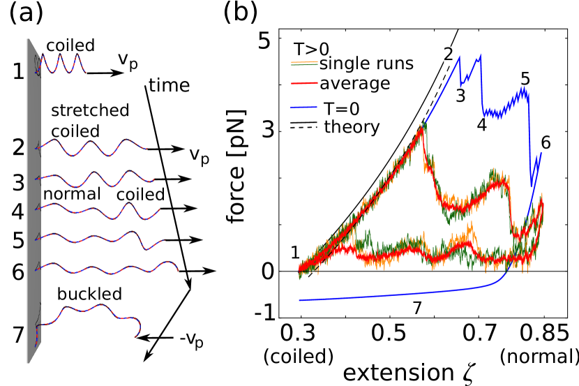
Figure 4: (a) Snapshots of a helical filament stretched at $T=0$ with velocity $v_{p}=2\mu\mathrm{m}/\mathrm{s}$ taken from the supplementary movie 1. The coiled-to-normal transition ($v_{p}>0$) and buckling ($v_{p}<0$) are visible. (b) Force-extension curves simulated without thermal noise ($T=0$) (blue curve) and with thermal noise: two realizations (thin orange and green lines) and an average over 10 runs (thick red line) are shown. The parameters are $v_{p}=2\mu\mathrm{m}/\mathrm{s}$ and $\Gamma=0.7$. Analytic prediction for a uniformly stretched filament (thin black line) and shifted curve (dashed black line).

We first simulated the extension of a filament with only one helical state. Similar to the snapshots 1 and 2 in Fig. 4(a) the deformation of the filament is uniform except for small regions at both ends. This leads to a small deviation of the simulated force-extension curve from the theoretical prediction of Eq. (16) for a uniformly stretched filament. The situation is similar to the results in Fig. 4(b), where the initial part 1-2 of the simulated blue curve is compared to the analytic prediction (thin black line). If we even shift the thin black line to the right, the dashed black line agrees very well with the blue curve besides the initial part close to position 1. We checked that even this difference gradually vanishes with increasing height of the helix as expected. In Section 2.6 we already explained that our simulations are performed in the quasistationary regime. This is also confirmed by our observation that at an extension rate $v_{p}=2\mathrm{\SIUnitSymbolMicro}\mathrm{m}\mathrm{/}\mathrm{s}$ the dissipated energy during one extension-and-compression cycle is only about $2\%$ of the maximum elastic energy at extension $\zeta_{M}$. Furthermore, we do not observe any pronounced difference between deterministic Stokesian and Brownian dynamics simulations. For $T\neq 0$, the forces fluctuate around a value which agrees with the deterministic force at $T=0$.

We then determined the force-extension curve at $T=0$ when the helical filament can switch from the coiled to the normal state using the elastic free energy (7). The results are illustrated in Fig. 4, where the blue curve in (b) corresponds to $T=0$. At a certain extension (position 2) the measured force drops sharply since a small segment of the filament close to the fixed end switches into the normal state as snapshots 2 and 3 in Fig. 4(a) reveal. Then the filament is stretched again. Further adjacent segments transform suddenly until at position 6 the filament is nearly completely in the normal state. From here we invert the velocity $v_{p}$ and move both ends together. However, the filament does not transform back into the coiled state but remains in the normal state. This ultimately leads to a negative force under which the filament buckles [see snapshot 7 in Fig. 4(a)]. The full cycle is shown in the supplementary movie 1.

Brownian dynamics simulations reveal the influence of thermal fluctuations on the force-extension curve. Two realizations are included in Fig. 4(b) as thin lines and the thick red line shows an ensemble average over 10 runs. A full cycle of one realization is shown in the supplementary movie 2. Clearly, the first transition into the normal state occurs at a smaller extension compared to the deterministic case since thermal fluctuations help to overcome the energy barrier in the elastic free energy density (see Fig. 3). Whereas the force in each realization fluctuates visibly, the sharp decrease of the force when a local transition into the normal state occurs is as pronounced as in the deterministic case. Finally, when both ends of the filament are moved together, it completely transforms back to the coiled state and buckling is not observed. The single realizations of the complete cycle of the force-extension curve closely resemble the experimental curves in Figs. 5 and 6 of Ref. Darnton07 . In particular, the force and extension where the first coiled-to-normal transition occurs fall into the experimental ranges of 3 to 5 pN and $\zeta=0.55$ to 0.6, respectively.

We now discuss in more detail how the difference $\delta$ in the ground-state energies of the two helical states, the twist-bend ratio $\Gamma$, and the extension rate $v_{p}$ influence the force-extension curves.

3.1.1 Ground-state energy difference $\delta$ of the coiled and normal state

Increasing the ground-state energy $\delta>0$ of the normal relative to the coiled state also increases the energy barrier, which the flagellum in the coiled configuration has to overcome to transform locally into the normal state. Therefore, the transition is delayed to a larger extension $z/L$ or does not occur at all. On the other hand, the barrier which the normal configuration has to overcome to relax back into the coiled state decreases and buckling of the filament becomes less probable. Observations also show that a filament prepared in the normal state very slowly relaxes back into the coiled state, so $\delta$ should not be too large compared to thermal energy $k_{B}T$. Using also the following quantitative considerations, we adjusted $\delta$ to $0.1\mathrm{p}\mathrm{N}$ which resulted in the good agreement with experimental observations, already demonstrated.

We now derive an upper bound for $\delta$ to ensure that a transformation from the coiled to the normal state is, in principal, observable. The locus of the energy barrier in the $\kappa,\tau$ plane of Fig. 3 is given by

$$f_{cl}(\boldsymbol{\Omega},\boldsymbol{\Omega}_{1})=f_{cl}(\boldsymbol{\Omega},\boldsymbol{\Omega}_{2})+\delta,$$ (19)

where $\boldsymbol{\Omega}=(0,\kappa,\tau)$ and $\boldsymbol{\Omega}_{i}=(0,\kappa_{i},\tau_{i})$ contains the values for spontaneous bend $\kappa_{i}$ and torsion $\tau_{i}$ of the coiled ($i=1$) and normal state ($i=2$), respectively. Assuming both states have the same elastic constants $A$, $C$, we arrive at a straight line

$$\kappa(\kappa_{1}-\kappa_{2})+\tau\Gamma(\tau_{1}-\tau_{2})+\delta/A$$

$$=(\kappa_{1}^{2}-\kappa_{2}^{2})/2+\Gamma(\tau_{1}^{2}-\tau_{2}^{2})/2.$$ (20)

We will use this formula later. The ground-state energy density of the normal state at $\boldsymbol{\Omega}_{2}=(0,\kappa_{2},\tau_{2})$ is $\delta$. Only if $\delta$ lies below the energy density of the coiled state at $\boldsymbol{\Omega}=\boldsymbol{\Omega}_{2}$ is a clear transition between both states possible. The explicit form of this upper bound, $\delta<f_{cl}(\boldsymbol{\Omega}_{2},\boldsymbol{\Omega}_{1})$, combines with $\delta>0$ to the inequality

$$0<\frac{\delta}{A(\kappa_{1}-\kappa_{2})^{2}}< (1+\Gamma\Delta^{2})/2,$$ (21)

where

$$\Delta=\frac{\tau_{1}-\tau_{2}}{\kappa_{1}-\kappa_{2}}$$ (22)

is the ratio of the differences in spontaneous torsion and curvature.

In experiments the value of $\delta$ changes with the conditions of the solvent. In particular, different polymorphic forms of the bacterial flagellum become stable when one alters the pH value, ionic strength, or temperature of the aqueous environment Hasegawa82 . It would be interesting to perform the force-extension experiments under different conditions to investigate how a changing $\delta$ but also variations in bending ($A$) and torsional ($C$) rigidity influence the force-extension curve of a bacterial flagellum.

3.1.2 Twist-to-bend ratio $\Gamma$

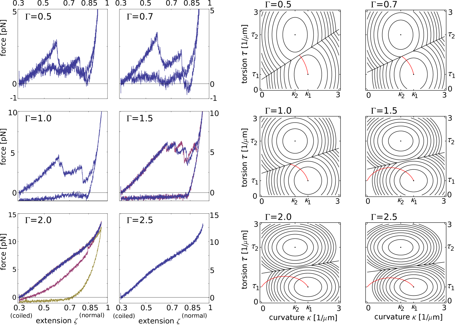
Figure 5: (a) One or several realizations of force-extension curves for increasing twist-to-bend ratios $\Gamma$. The extensional rate is $v_{p}=2\mu\mathrm{m}/\mathrm{s}$. (b) Contour plots of the elastic free energy density as a function of curvature and torsion for the same $\Gamma$ as in (a). The red line indicates the sequence of $\kappa,\tau$ values, as the filament in the coiled state is uniformly stretched.

Increasing the twist-to-bend ratio $\Gamma$ also increases the energy barrier as the following formula for the minimum value of the barrier demonstrates,

$$\frac{f_{b}}{A(\kappa_{1}-\kappa_{2})^{2}}= \frac{\left(1+2\delta/[A(\kappa_{1}-\kappa_{2})^{2}]+\Gamma\Delta^{2}\right)^{2}}{8\left(1+\Gamma\Delta^{2}\right)}.$$ (23)

However, in contrast to $\delta$ an increasing $\Gamma$ increases both barriers for the coiled-to-normal and the normal-to-coiled transition. We now discuss in Fig. 5(a) how the twist-to-bend ratio $\Gamma$ influences the force-extension curve of the helical filament. The filament is stretched to an extension $\zeta=0.95$, well above the equilibrium height $\zeta=0.85$ of the normal state. Fig. 5(b) shows contour plots of the elastic free energy density as a function of curvature and torsion for the same $\Gamma$ as in (a). The red line indicates the sequence of $\kappa,\tau$ values, as the filament in the coiled state is uniformly stretched (see Section 2.5). Note that for $\Gamma\neq 1$ the anisotropy of the elastic free energy density is clearly visible.

For $\Gamma=0.5$ and $0.7$, one observes the typical force-extension curves as already discussed in Fig. 4 also for $\Gamma=0.7$. Since now the maximal extension $\zeta=0.95$ is larger, the curve for $\Gamma=0.7$ during compression looks different. While at $\zeta=0.95$ the entire filament is in the normal state, the filament for $\Gamma=1$ no longer transforms completely into the normal state. Most pronounced at $\Gamma=1$ is the fact that even with thermal forces the filament does not return into the coiled state during compression. This results in a negative force under which the filament buckles. All the force-extension curves in Fig. 5(a) are determined for an extension rate $v_{p}=2\mathrm{\SIUnitSymbolMicro}\mathrm{m}\mathrm{/}\mathrm{s}$. A smaller $v_{p}$ enhances the probability that thermal fluctuations transform the filament back into the coiled state and buckling is not observed. The same is true for a smaller extension where a larger part of the filament stays in the coiled state and makes it easier for the rest of the filament to return to the coiled state. At a ratio $\Gamma=1.5$ the force-extension curve changes qualitatively. A first transition into the normal state occurs at a larger extension $\zeta\approx 0.65$ compared to the previous curves. The transitions are no longer as pronounced and there are larger differences between single realizations of the force-extension curve. In addition, for $\Gamma<1.5$ only one normal domain occurs whereas for $\Gamma=1.5$ two normal domains are observed. The reason for all these features becomes clear from Fig. 5(b). At $\Gamma=1.5$ a uniformly stretched filament does not hit the energy barrier anymore but passes the barrier in a close distance so that thermal fluctuations are needed to induce transformations into the normal state. For further increase of $\Gamma$ a transition into the normal state does not occur at all realizations, as the three graphs for $\Gamma=2$ demonstrate. A similar behavior is observed in Ref. Darnton07 for a transition from the normal into the hyperextended state. The blue curve corresponds to the traditional force-extension relation of the helix in the coiled state. In the yellow curve a complete transition into the normal state was realized. A partial transformation occurred in the magenta curve which then completely returned into the coiled state. Finally, at $\Gamma=2.5$ the filament always remains in the coiled state. Beyond an extension of $\zeta=0.5$ the slope of the curve becomes smaller. This is the onset of a qualitatively new behavior. At even larger $\Gamma$ and $\tau_{0}/\kappa_{0}<1$, one observes a sharp drop in the force due to a discontinuous transformation, where one turn of the helical filament unwinds. This is discussed in Refs. Kessler2003 ; Wada2007a .

As discussed, neglecting thermal fluctuations, a coiled-to-normal transition is no longer observable in the force-extension curve when in Fig. 5(b) the straight line [Eq. (20)] separating the coiled and normal state becomes tangential to the trajectory [Eq. (17)] of the uniformly stretched filament. Combining both equations leads to a second condition for $\delta/A$:

$$\frac{\delta}{A(\kappa_{1}-\kappa_{2})^{2}} <\frac{1}{2(\kappa_{1}-\kappa_{2})}\bigg{(}\kappa_{2}+\Gamma\tau_{2}\Delta$$

$$\qquad\qquad+\sqrt{(1+\Gamma\Delta^{2})(\kappa_{1}^{2}+\Gamma\tau_{1}^{2})}\bigg{)}$$ (24)

Together with condition (21), we obtain a region in the parameter space $(\Gamma,\delta/A)$ where a transformation from the coiled to the normal state should occur. The region is indicated as shaded area in Fig. 6. Based on experimental data for Young’s and shear modulus in literature, Flynn and Ma received for the twist-to-bend ratio $\Gamma$ the range $2\cdot 10^{-1}-2\cdot 10^{2}$ Flynn2004 . With a computational method, called the quantized elastic deformational model, they calculated $\Gamma\approx 23$ Flynn2004 . On the other hand, together with our value $\delta/[A(\kappa_{1}-\kappa_{2})^{2}]\approx 0.11$, we predict a value of $\Gamma\lesssim 1$, in good agreement with our simulations.

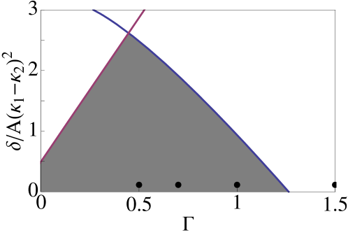
Figure 6: The shaded area indicates the parameter ranges for the ground-state energy difference $\delta$ and the twist-to-bend ratio $\Gamma$ for which a coiled-to-normal transition should be observed. The dots give parameter values used in simulations. Note that thermal fluctuations shift the upper border for $\Gamma$ indicated by the blue line to the right.

3.1.3 Extensional rate

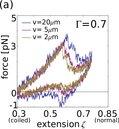
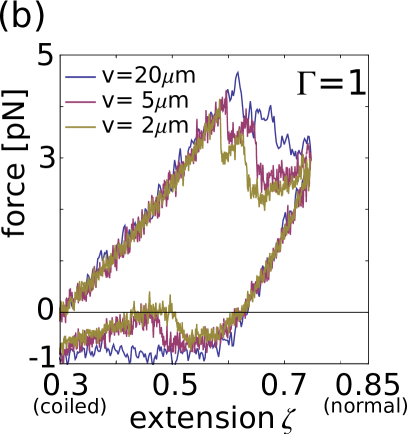
Figure 7: Force-extension curves for twist-to-bend ratios $\Gamma=0.7$ (a) and $\Gamma=1$ (b) at different extension rates $v_{p}=2\mathrm{\SIUnitSymbolMicro}\mathrm{m}\mathrm{/}\mathrm{s}$, $5\mathrm{\SIUnitSymbolMicro}\mathrm{m}\mathrm{/}\mathrm{s}$ and $20\mathrm{\SIUnitSymbolMicro}\mathrm{m}\mathrm{/}\mathrm{s}$.

In Section 2.6 we reasoned that during the measurements of the force-extension curves the bacterial flagellum goes through a sequence of equilibrium states. This means that frictional forces acting on the filament through the solvent are negligible against elastic forces. Therefore, without thermal noise, the force-extension curve does not depend on the extensional rate $v_{p}$. In contrast, our Brownian dynamics simulations demonstrate a clear influence of $v_{p}$. In Fig. 7, we show force-extension curves for twist-to-bend ratios $\Gamma=0.7$ and $1$ and different extension rates $v_{p}=2\mathrm{\SIUnitSymbolMicro}\mathrm{m}\mathrm{/}\mathrm{s}$, $5\mathrm{\SIUnitSymbolMicro}\mathrm{m}\mathrm{/}\mathrm{s}$ and $20\mathrm{\SIUnitSymbolMicro}\mathrm{m}\mathrm{/}\mathrm{s}$. The first transition from the coiled to normal state occurs at larger extensions when $v_{p}$ is increased. This is immediately clear since smaller velocities $v_{p}$ give the filament more time to explore the energy landscape with the help of thermal fluctuations. So the appropriate local curvature and torsion to overcome the potential barrier can be created at smaller extension. The curves in Fig. 7 just give one specific realization for each parameter set. In the following section, we will investigate in detail the probability distribution for the extension where the first coiled-to-normal transition occurs.

If the filament in the normal state is compressed too fast, it will start to buckle since again it has not sufficient time to overcome the energy barrier. This is visible in Fig. 7(a), where the filament with the highest compressing rate $v_{p}=20\mu\mathrm{m/s}$ buckles which corresponds to a negative force. On the other hand, for smaller rates $v_{p}$, the filament always returns into the coiled state.

3.2 Clamped filament

Since the bacterial flagellum goes through a sequence of equilibrium states during the measurements of the force-extension curves, it should be possible to derive some characteristics of these curves by investigating a clamped filament which is hold at a fixed extension $\zeta=z/L$ in thermal equilibrium. In particular, we show here how one can infer the mean extension $\langle\zeta\rangle(v_{p})$ at which the filament in a force-extension measurement undergoes the first local transition to the normal state

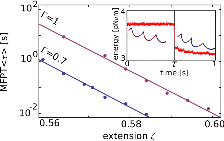
Figure 8: Mean-first-passage time (MFPT) as a function of extension $\zeta$ for $\Gamma=0.7$ and $\Gamma=1.0$. Inset: When the local coiled-to-normal transition occurs, the energy decreases instantaneously.

We stretch the filament in the coiled state at zero temperature to an extension $\zeta$ and keep this extension constant. We then perform a Brownian dynamics simulation and determine for each realization the first-passage time $\tau$ at which a local transition to the normal state occurs. The inset of Fig. 8 shows the filament before and after the transition accompanied by a sharp decrease of the elastic free energy. According to Kramers theory, the mean-first-passage time (MFPT) is proportional to the Arrhenius factor,

$$\left\langle\tau\right\rangle\sim \exp\left(\frac{\triangle\mathcal{F}(\zeta)}{k_{B}T}\right).$$ (25)

The activation energy $\triangle\mathcal{F}(\zeta)$ depends on the extension $\zeta$ and is needed to create the domain wall between the coiled and normal state. We determined the MFPT by averaging over 100 simulated values for $\tau$ at each extension $\zeta$. The results are plotted in Fig. 8 for two twist-to-bend ratios $\Gamma=0.7$ and $\Gamma=1$. We only simulated $\left\langle\tau\right\rangle$ for a small variation in the extension for two reasons: at larger extensions where $\triangle\mathcal{F}(\zeta)\approx k_{B}T$ the Kramers theory is no longer valid and $\left\langle\tau\right\rangle$ is too small to be determined accurately; at smaller extensions $\left\langle\tau\right\rangle$ is so large that it cannot be calculated in reasonable simulation times. Note that for $\Gamma=1$ the MFPT spans three decades. Our simulation results demonstrate that $\log\left\langle\tau\right\rangle(\zeta)$ can be fitted by

$$\log\left\langle\tau\right\rangle(\zeta)\approx\alpha-\beta\zeta,$$ (26)

where $\left\langle\tau\right\rangle$ is measured in seconds. Equation (26) can just be viewed as a Taylor expansion to linear order in $\zeta$. The parameters $\alpha$ and $\beta$ follow from a least-square fit. Whereas $\alpha$ changes with $\Gamma$, the slope $\beta$ surprisingly does not seem to depend on $\Gamma$ within the numerical accuracy. A similar law as Eq. (26) is used in situations where bonds rupture under a given load force Evans2001 ; Bell1978 . Note, however, that here we control the extension.

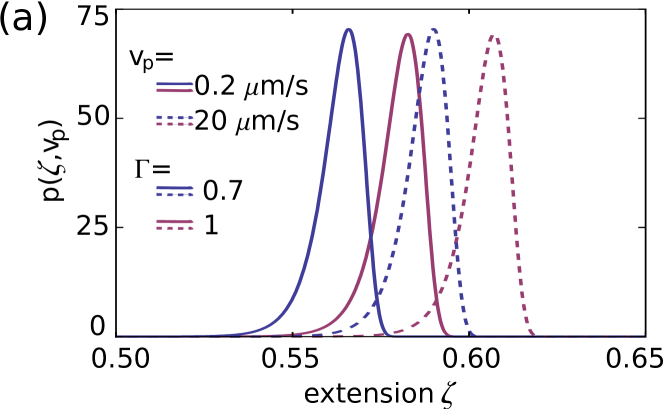
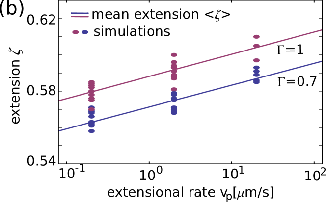
Figure 9: (a) Probability distributions $p(\zeta,v_{p})$ as a function of extension $\zeta$ for $\Gamma=0.7$ (blue) and $\Gamma=1$ (magenta) at extension rates $v_{p}=0.2\mathrm{\SIUnitSymbolMicro}\mathrm{m}\mathrm{/}\mathrm{s}$ (full lines) and $v_{p}=20\mathrm{\SIUnitSymbolMicro}\mathrm{m}\mathrm{/}\mathrm{s}$ (dashed lines). (b) Analytically determined mean extension $\left\langle\zeta\right\rangle(v_{p})$ for the coiled-to-normal transition as a function of velocity $v_{p}$ for $\Gamma=0.7$ (blue) and $\Gamma=1$ (magenta). The dots indicate numerically determined extensions for each simulation run.

Within the adiabatic or quasistationary approximation, we now formulate the probability $p(t,v_{p})\text{d}t$ that within the time interval $[t,t+\text{d}t]$ the filament transforms locally from the coiled to normal state when stretched with velocity $v_{p}$,

$$p(t,v_{p}) =\frac{1}{\left\langle\tau\right\rangle(\zeta(t,v_{p}))}\exp\left(-\int_{0}^{t}1/\left\langle\tau\right\rangle(\zeta(t^{\prime},v_{p}))\text{d}t^{\prime}\right),$$ (27)

where

$$\zeta(t,v_{p})=\zeta_{0}+tv_{p}/L$$ (28)

is the extension at time $t$. The exponential factor in Eq. (27) is the probability that until time $t$ a transition does not occur, which follows by writing the probability that a transition within the time interval $\text{d}t^{\prime}$ does not happen as $(1-\text{d}t^{\prime}/\left\langle\tau\right\rangle)\approx\exp(-\text{d}t^{\prime}/\left\langle\tau\right\rangle)$. The first factor is the probability per unit time that the transition occurs within $\text{d}t$ at time $t$ when the filament is with certainty in the coiled state before. Using Eq. (28), one introduces the probability $p(\zeta,v_{p})\text{d}\zeta=p(t,v_{p})\text{d}t$ that the filament undergoes a local coiled-to-normal transition at extension $\zeta$. We calculate it analytically in Appendix D by assuming the validity of Eq. (26) for the whole $\zeta$ range. The results are plotted in Fig. 9(a) for $\Gamma=0.7$ (blue) and $\Gamma=1$ (magenta) and for extension rates $v_{p}=0.2\mathrm{\SIUnitSymbolMicro}\mathrm{m}\mathrm{/}\mathrm{s}$ (full lines) and $v_{p}=20\mathrm{\SIUnitSymbolMicro}\mathrm{m}\mathrm{/}\mathrm{s}$ (dashed lines). The probability distributions are concentrated on a small range about their maximum values and are shifted to larger extensions for increasing velocities $v_{p}$, as expected. We then calculate the mean extension

$$\left\langle\zeta\right\rangle(v_{p})=\int_{\zeta_{0}}^{\infty}\zeta^{\prime}p(\zeta^{\prime},v_{p})d\zeta^{\prime},$$ (29)

at which the coiled-normal transition occurs first for a given extension rate $v_{p}$. The evaluation of the integral is performed in Appendix D and finally gives

$$\left\langle\zeta\right\rangle(v_{p})\propto\log v_{p}.$$ (30)

The mean extension $\left\langle\zeta\right\rangle(v_{p})$ with all prefactors and constant terms is plotted in Fig. 9(b) for $\Gamma=0.7$ (blue) and $\Gamma=1$ (magenta) together with numerically determined extensions $\zeta$ for several realizations at a specific velocity $v_{p}$. The values scatter around the mean value and are, therefore, in good agreement with the analytical treatment. We note that a relation similar to Eq. (30) occurs for the velocity dependence of the rupture force of single molecular bonds in dynamic force spectroscopy Evans2001 .

4 Summary and conclusions

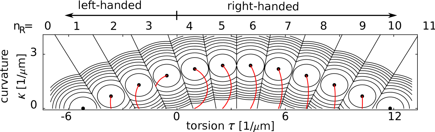
Figure 10: Contour lines of the free energy density of the extended Kirchhoff rod theory that includes all 12 polymorphic states of the bacterial flagellum. For all helical states the same ground state energy and the same bending and torsional rigidity with $\Gamma=0.7$ is assumed. The red lines indicate the paths of uniformly stretched flagella.

In this article we have developed a sufficiently simple elastic model to describe the polymorphism of a bacterial flagellum based on Kirchhoff’s theory of an elastic rod. The friction with the aqueous environment is modeled within resistive force theory. Using geometrical parameters of the coiled and normal states and the bending rigidity as obtained in Ref. Darnton07 , we are able to reproduce the force-extension curves recorded in experiments. Thermal fluctuations realized within Brownian dynamics simulations are crucial. In particular, the force values at which a first coiled-to-normal transition takes place lie between 3 and 5 pN, as in experiments Darnton07 . We have investigated in detail how the force-extension curve depends on the twist-to-bend ratio $\Gamma$ and, furthermore, by analytic arguments identified a parameter region for ground-state energy difference $\delta$ and $\Gamma$, where a coiled-to-normal transition should be observable. It clearly demonstrates that for values of $\Gamma$ well above one, a polymorphic transformation is not possible and therefore contradicts some of the experimental values for $\Gamma$ recorded in literature. Based on our simulations, we predict $\Gamma$ to be within $0.7$ and $1.0$. Further studies demonstrate how the extensional rate $v_{p}$ influences the force extension curve. We directly observe the influence in the simulations of the full force-extension cycle but also when we concentrate on the extension for the first coiled-to-normal transition. Since the extensional rates $v_{p}$ are sufficiently small, the flagellum goes through a sequence of quasi-stationary states. We, therefore, used equilibrium properties of clamped flagella to predict a logarithmic velocity dependence for the mean extension of the first coiled-to-normal transition in good agreement with our simulations.

Our approach is easily extended to include more than two polymorphic states. Figure 10 shows the contour lines of the resulting free energy landscape when all twelve polymorphic conformations of Fig. 1 are taken into account. For each of these conformations we take Kirchhoff’s elastic free energy with spontaneous curvature and torsion as given by Calladine Calladine75 and just consider the minimum value from all these free energies. We assume here that the ground-state energies of all helical states are zero and that they all have the same bending and torsional rigidities with $\Gamma=0.7$. We also included the paths of uniformly stretched helical filaments. The coiled-to-normal transition ($n_{R}=3$ to 2) takes place with certainty. However, all the other transitions would need thermal fluctuations to occur. For example, the normal-to-hyperextended transition ($n_{R}=2$ to 1) will only occur when it is stretched sufficiently slowly so that thermal fluctuations can induce the transformation.

We can now use our model to study various aspects connected to bacterial locomotion. For example, we will investigate how polymorphic transitions are induced by rotating the flagellum. Our very challenging goal is to model the complete tumbling cycle of a bacterium. Finally, we note that our model may be applicable as well to spirochetes, where very recent experiments and theory have begun to address the elasticity of the helical structure Dombrowski2009 .

Appendix A Extended Kirchhoff rod theory: the double-well potential

Here, the main idea is to extend the theory of Goldstein et al. Goldstein2000 ; Coombs2002 . They used a double well potential for the twist density $\Omega_{3}$, realized by a polynomial of degree four, to describe two polymorphic states of a flagellum Goldstein2000 ; Coombs2002 .

In order to develop a strategy how to generalize this double well potential to all three coordinates $\Omega_{i}$ ($i=1,2,3$), we first write down a general one-dimensional polynomial of degree four:

$$f(x,x_{1},x_{2}) =\frac{A}{2}\frac{(x-x_{1})^{2}}{(x_{1}-x_{2})^{2}}[(x-x_{2})^{2}$$

$$\qquad-\frac{d}{6}(x-x_{1})(3x+x_{1}-4x_{2})].$$ (31)

For $d<1$ it has two minima at $x_{1}$ and $x_{2}$ with $f(x_{1})=0$ and $f(x_{2})=\delta$, respectively, where

$$\delta =\frac{1}{12}A(x_{1}-x_{2})^{2}d.$$ (32)

Whereas $\partial_{x}^{2}f(x_{1})=A$, the second derivative at $x_{2}$ depends on the parameters $x_{1}$, $x_{2}$, $d$, and $A$.

We generalize the polynomial of Eq. (31) to three dimensions by replacing terms of the form $Axy$ by $\boldsymbol{x}\cdot\boldsymbol{\sf A}\boldsymbol{y}$, where $\boldsymbol{x}$, $\boldsymbol{y}$ are three-dimensional vectors and $\boldsymbol{\sf A}$ is a diagonal matrix with $A_{11}=A_{22}=A$ and $A_{33}=C$. The constants $A$, $C$ are the bending and torsional rigidities, respectively. Using the shorthand notation $|\boldsymbol{x}|^{2}_{\boldsymbol{\sf A}}=\boldsymbol{x}\cdot\boldsymbol{\sf A}\boldsymbol{x}$ with $\boldsymbol{x}=\boldsymbol{\Omega}-\boldsymbol{\Omega}_{i}$, we now write

$$f(\boldsymbol{\Omega},\boldsymbol{\Omega}_{1},\boldsymbol{\Omega}_{2}) =\frac{1}{2}\frac{|\boldsymbol{\Omega}-\boldsymbol{\Omega}_{1}|_{\boldsymbol{\sf A}}^{2}}{|\boldsymbol{\Omega}_{1}-\boldsymbol{\Omega}_{2}|_{\boldsymbol{\sf A}}^{2}}[|\boldsymbol{\Omega}-\boldsymbol{\Omega}_{2}|_{\boldsymbol{\sf A}}^{2}$$

$$\quad-\frac{d}{6}(\boldsymbol{\Omega}-\boldsymbol{\Omega}_{1})\cdot\boldsymbol{\sf A}(3\boldsymbol{\Omega}+\boldsymbol{\Omega}_{1}-4\boldsymbol{\Omega}_{2})]$$ (33)

$$\text{with}\enspace\delta =\frac{1}{12}|\boldsymbol{\Omega}_{1}-\boldsymbol{\Omega}_{2}|_{\boldsymbol{\sf A}}^{2}d.$$ (34)

The polynomial is illustrated in Fig. 11(a) with $\boldsymbol{\Omega}=(0,\kappa,\tau)$. It has two minima at $\boldsymbol{\Omega}_{1}$, $\boldsymbol{\Omega}_{2}$ with $f(\boldsymbol{\Omega}_{1})=0$, $f(\boldsymbol{\Omega}_{2})=\delta$, respectively, and one saddle point at $\boldsymbol{\Omega}_{3}=\boldsymbol{\Omega}_{1}+\frac{1}{2-d}(\boldsymbol{\Omega}_{2}-\boldsymbol{\Omega}_{1})$ for $d<1$. Close to the first minimum at $\boldsymbol{\Omega}_{1}$, the polynomial agrees with Kirchhoff’s elastic free energy (4), whereas the bending and torsional rigidities at $\boldsymbol{\Omega}_{2}$ and also the energy barrier depend on $\delta$.

Figure 11(b) shows a force-extension curve (red line) simulated with Eq. (33) at $T=0$ for the same parameters as in Fig. 5(a) with $\Gamma=1$. For comparison the initial part of the curve from Fig. 5(a) ($\Gamma=1$) is included. The helical filament is much softer and the initial part of the force-extension relation has a negative curvature in contrast to experiments. We, therefore, decided to introduce the alternative model of Eq. (5).

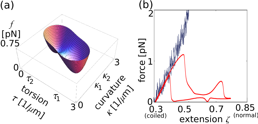
Figure 11: (a) Double-well potential of Eq. (33) plotted as a function of $\Omega_{2}=\kappa$ and $\Omega_{3}=\tau$ for the parameters of the coiled and normal helical state. (b) Force-extension curve (red line) simulated with this potential at $T=0$ and $v_{p}=2\mathrm{\SIUnitSymbolMicro}\mathrm{m}\mathrm{/}\mathrm{s}$. The blue curve is taken from Fig. 5(a) for the same parameter $\Gamma=1$.

Appendix B Simplifying the free energy of Wada and Netz

After integrating out the spin degree of freedom, Wada and Netz arrived at the following elastic free energy density Wada2008 :

$$f(\boldsymbol{\Omega},\boldsymbol{\Omega}_{1},\boldsymbol{\Omega}_{2}) =f_{1}-f_{2}$$ (35)

with

$$f_{1}= \frac{A}{2}\Omega_{1}^{2}+\frac{A}{2}\left(\Omega_{2}-\frac{\kappa_{1}+\kappa_{2}}{2}\right)^{2}+\frac{C}{2}\left(\Omega_{3}-\frac{\tau_{1}+\tau_{2}}{2}\right)^{2}$$ (36)

$$f_{2}= \frac{k_{B}T}{a}\ln\Big{[}\cosh(\Lambda)+\sqrt{\sinh^{2}(\Lambda)+\text{e}^{-4J/k_{B}T}}\Big{]}+\frac{J}{a}$$ (37)

and

$$\frac{k_{B}T}{a}\Lambda= \delta+\frac{A}{2}(\kappa_{1}-\kappa_{2})\left(\Omega_{2}-\frac{\kappa_{1}+\kappa_{2}}{2}\right)$$

$$\qquad\qquad+\frac{C}{2}(\tau_{1}-\tau_{2})\left(\Omega_{3}-\frac{\tau_{1}+\tau_{2}}{2}\right)$$ (38)

Here $A,C$ are the bending and torsional rigidities, respectively, $\delta$ is the difference of the ground-state energies of the helical conformations $(\kappa_{1},\tau_{1})$ and $(\kappa_{2},\tau_{2})$, and $a$ the length of discretization. The quantity $J$ is the interaction strength in the Ising Hamiltonian.

We interpret the energy cost $2J$ for two anti-parallel spins as the energy of a domain wall connecting two helical states. Since such domain walls are rarely seen in experiments Hasegawa82 , we can assume $2J\gg k_{B}T$ and, therefore, approximate $f_{2}$ as

$$f_{2} \approx\frac{k_{B}T}{a}|\Lambda|+\frac{J}{a},$$ (39)

where we have used $\cosh x+|\sinh x|=\exp|x|$. Now, we introduce the elastic free energy densities of the two helical states,

$$\alpha =\frac{A}{2}\Omega_{1}^{2}+\frac{A}{2}\left(\Omega_{2}-\kappa_{2}\right)^{2}+\frac{C}{2}\left(\Omega_{3}-\tau_{2}\right)^{2}+\delta/2,$$ (40)

$$\beta =\frac{A}{2}\Omega_{1}^{2}+\frac{A}{2}\left(\Omega_{2}-\kappa_{1}\right)^{2}+\frac{C}{2}\left(\Omega_{3}-\tau_{1}\right)^{2}-\delta/2,$$ (41)

and write the two contributions to the energy density (35) as

$$f_{1}= \frac{1}{2}(\alpha+\beta)+c_{1}, f_{2}\approx \frac{1}{2}|\alpha-\beta|+\frac{J}{a},$$ (42)

where $c_{1}$ is just a constant. This finally gives our ansatz for the free energy density (5):

$$f\approx \frac{1}{2}(\alpha+\beta-|\alpha-\beta|)+c_{1}=\min(\alpha,\beta)+c_{1}.$$ (43)

Appendix C Friction coefficients per unit length

In a moving helical filament, different parts interact via hydrodynamic interactions. Nevertheless, using slender-body theory, Lighthill demonstrated that one can describe the hydrodynamic friction of the filament with the help of resistive force theory that introduces local friction coefficients per unit length. For the translational coefficients, Lighthill obtained Lighthill1976

$$\gamma_{\parallel} =\frac{2\pi\eta}{\ln(2q/r)}\enspace\mathrm{and}\enspace\gamma_{\perp}=\frac{4\pi\eta}{\ln(2q/r)+1/2}.$$ (44)

Here $\eta$ is the shear viscosity, $r=0.02\mathrm{\SIUnitSymbolMicro}\mathrm{m}$ the cross-sectional radius of the bacterial flagellum, and $q$ a characteristic length, for which Lighthill derived $q=0.09\Lambda$, where $\Lambda=2\pi/\sqrt{\kappa^{2}+\tau^{2}}$ is the filament length of one helical turn. This gives $\gamma_{\parallel}\approx 1.54\eta$, $\gamma_{\perp}\approx 2.74\eta$ for the normal state and $\gamma_{\parallel}\approx 1.64\eta$, $\gamma_{\perp}\approx 2.91\eta$ for the coiled state. Since the coefficients are similar in both states, we use the intermediate values $\gamma_{\parallel}\approx 1.6\eta$ and $\gamma_{\perp}\approx 2.8\eta$ for simulating the force-extension curves. Finally, for the rotational friction coefficient one finds Brennen1977

$$\gamma_{R} =4\pi\mu a^{2}.$$ (45)

Appendix D Velocity dependence of the mean extension $\left\langle\zeta\right\rangle(v_{p})$

In the following we use the numerically determined MFPT of Eq. (26) in the form

$$\left\langle\tau\right\rangle=\tau_{0}\exp[-\beta(\zeta-\zeta_{0})].$$ (46)

We transform the probability distribution $p(t)$ in Eq. (27) into a probability distribution for the rescaled extension variable $x=\beta(\zeta-\zeta_{0})=\beta v_{p}t/L$ using $p(t)\text{d}t=p(x)\text{d}x$. The integral in Eq. (27) is readily calculated with the help of $\left\langle\tau\right\rangle=\tau_{0}\exp(-x)$ and we obtain

$$p(x)\text{d}x=\text{e}^{x-A}\exp\left(-\text{e}^{-A}(\text{e}^{x}-1)\right)\text{d}x,$$ (47)

where $\exp(-A)=L/(\beta v_{p}\tau_{0})$. At $x=0$ or $\zeta=\zeta_{0}$, the choice of our parameters shows that the energy barrier between coiled and normal state is much larger than $k_{B}T$, so $p(x=0)=e^{-A}$ is almost zero or $A\gg 1$. Even for $x\approx 0$, we can therefore approximate the probability density in Eq. (47) as

$$p(x)\approx\text{e}^{x-A}\exp\left(-\text{e}^{x-A}\right)\text{d}x:=p_{0}(x-A).$$ (48)

It explains why all the probability densities $p(\zeta,v_{P})$ in Fig. 9 have the same shape but are shifted relative to each other along the $\zeta$ axis due to different values of $v_{p}$ and $\Gamma$ and, therefore, of $A$. The distribution $p(x)$ has a maximum at $x=A$ with $p(A)\approx e^{-1}$.

We now calculate the rescaled mean extension

$$\left\langle x\right\rangle =\int_{0}^{\infty}xp(x)\text{d}x.$$ (49)

We rewrite the probability distribution of Eq. (48) as $p(x)=\text{e}^{x-A}\exp\left(-\text{e}^{x-A}\right)=-\partial_{x}\exp\left(-\text{e}^{x-A}\right)$ and obtain after integrating by parts

$$\left\langle x\right\rangle =\exp(\text{e}^{-A})\int_{0}^{\infty}\exp\left(-\text{e}^{x-A}\right)\text{d}x.$$ (50)

The substitution $y=-\exp(x-A)$ then introduces the exponential integral function:

$$\left\langle x\right\rangle =-\exp(\text{e}^{-A})\int_{-\infty}^{-\text{e}^{-A}}\frac{\text{e}^{y}}{y}\text{d}y,$$ (51)

which for $\text{e}^{-A}\ll 1$ is approximated by

$$\left\langle x\right\rangle \approx-(C+\log\text{e}^{-A})=-C+A,$$ (52)

where $C\approx 0.577$ is Euler’s constant. Introducing the original extension variable $\zeta$ and $A=\log(v_{p}\tau_{0}/L)+\log(\beta)$, we obtain for the mean extension at which the coiled-to-normal transition first takes place:

$$\beta(\left\langle\zeta\right\rangle-\zeta_{0})=-C+\log(v_{p}\tau_{0}/L)+\log(\beta)\propto\log(v_{p}).$$ (53)

References

- (1) H. C. Berg, E. coli in Motion, Springer Verlag, New York (2004).
- (2) L. Zhang, J.J. Abbott, L. Dong, B.E. Kratochvil, D. Bell, and B.J. Nelson, Appl. Phys. Lett. 94, 064107 (2009).
- (3) B. Behkam and M. Sitti, Appl. Phys. Lett. 90, 023902 (2007).
- (4) M.J. Kim and K.S. Breuer, Small 4, 111 (2008).
- (5) E. Barry, Z. Hensel, Z. Dogic, M. Shribak, and R. Oldenbourg, Phys. Rev. Lett. 96, 018305 (2006).
- (6) R. Kamiya and S. Asakura, J. Mol. Biol. 106, 167 (1976).
- (7) R. Kamiya and S. Asakura, J. Mol. Biol. 108, 513 (1977).
- (8) E. Hasegawa, R. Kamiya and S. Asakura, J. Mol. Biol. 160, 609 (1982).
- (9) H. Hotani, Biosystems 12, 325 (1980).
- (10) M. Seville, T. Ikeda, and H. Hotani, FEBS Lett. 332, 260 (1993).
- (11) R. M. Macnab and M. K. Ornston, J. Mol. Biol. 112, 1 (1977).
- (12) H. Hotani, J. Mol. Biol. 156, 791 (1982).
- (13) N. C. Darnton, L. Turner, S. Rojevsky, and H. C. Berg, J. Bacteriol. 189, 1756 (2007).
- (14) N. C. Darnton and H. C. Berg, Biophys. J. 92, 2230 (2007).
- (15) K. Hasegawa, I. Yamashita, and K. Namba, Biophys J 74, 569 (1998).
- (16) S. Asakura, Adv. Biophys. 1, 99 (1970).
- (17) C. R. Calladine, Nature 255, 121 (1975).
- (18) I. Yamashita, K. Hasegawa, H. Suzuki, F. Vonderviszt, Y. Mimori-Kiyosue, and K. Namba, Nat. Struct. Biol. 5, 125 (1998).
- (19) K. Yonekura, S. Maki-Yonekura, and K. Namba, Nature 424, 643 (2003).
- (20) S.V. Srigiriraju and T.R. Powers, Phys. Rev. Lett. 94, 248101 (2005).
- (21) S.V. Srigiriraju and T.R. Powers, Phys. Rev. E . 73, 011902 (2006).
- (22) B. Friedrich, J. Math. Biol. 53, 162 (2006).
- (23) C. Speier, Ising Model for Bacterial Flagella, diploma thesis, Technische Universität Berlin (2010).
- (24) A. Arkhipov, P. L. Freddolino, K. Imada, K. Namba, and K. Schulten, Biophys. J. 91, 4589 (2006).
- (25) R.E. Goldstein, A. Goriely, G. Huber, and C.W. Wolgemuth, Phys. Rev. Lett. 84, 1631 (2000).
- (26) D. Coombs, G. Huber, J.O. Kessler, and R.E. Goldstein, Phys. Rev. Lett. 89, 118102 (2002).
- (27) H. Wada and R.R. Netz, Europhys. Lett. 82, 28001 (2008).
- (28) A.E.H. Love, A Treatise on the Mathematical Theory of Elasticity (New York Dover Publications, 1944).
- (29) L. Landau and E. Lifshitz, Theory of Elasticity (Pergamon Press, 1986).
- (30) S. Childress, Mechanics of swimming and flying. (Cambridge University Press, 1981).
- (31) J. Lighthill, SIAM Rev. 18, 161 (1976).
- (32) E.M. Purcell, Am. J. Phys 45, 3 (1977).
- (33) S. Chattopadhyay, R. Moldovan, C. Yeung, and X.L. Wu, PNAS 103, 13712 (2006).
- (34) S. Chattopadhyay and X.L. Wu, Biophys. J. 96, 2023 (2009).
- (35) M. Reichert, Ph.D. thesis, University Konstanz (2006), http://nbn- resolving.de/urn:nbn:de:bsz:352-opus-19302.
- (36) G. Chirico and J. Langowski, Biopolymers 34, 415 (1994).
- (37) H. Wada and R.R. Netz, Europhys. Lett. 77, 68001 (2007).
- (38) H. Wada and R.R. Netz, Phys. Rev. Lett. 99, 108102 (2007).
- (39) D.A. Kessler and Y. Rabin, Phys. Rev. Lett. 90, 024301 (2003).
- (40) A. Goriely and M. Tabor, Proc. R. Soc. Lond. A, 453, 2583 (1997)
- (41) T.C. Flynn and J. Ma, Biophys. J. 86, 3204 (2004).
- (42) C. Brennen and H. Winet, Annu. Rev. Fluid Mech. 9, 339 (1977).
- (43) E. Evans, Annu. Rev. Biophys. Biomol. Struct. 30, 105 (2001).
- (44) C.W. Wolgemuth, T.R. Powers, and R.E. Goldstein, Phys. Rev. Lett., 84, 1623 (2000).
- (45) G. I. Bell, Science, 200, 618-627 (1978).
- (46) C. Dombrowski, W. Kan, M. A. Motaleb, N. W. Charon, R. E. Goldstein, and C. W. Wolgemuth, Biophys. J., 96, 4409 (2009)