1 Copyright

Alisa Krishtal¹, Patrick Senet², Christian Van Alsenoy¹ psenet@u-bourgogne.fr

Copyright 2009 American Institute of Physics. This article may be downloaded for personal use only. Any other use requires prior permission of the author and the American Institute of Physics. The following article appeard in J. Chem. Phys.  131, 044312 (2009) and may be found at
http://jcp.aip.org/resource/1/jcpsa6/v131/i4/p044312_s1

Local softness, softness dipole and polarizabilities of functional groups: application to the side chains of the twenty amino acids

Alisa Krishtal¹, Patrick Senet², Christian Van Alsenoy¹ psenet@u-bourgogne.fr

Abstract

The values of molecular polarizabilities and softnesses of the twenty amino acids were computed ab initio (MP2). By using the iterative Hirshfeld scheme to partition the molecular electronic properties, we demonstrate that the values of the softness of the side chain of the twenty amino acid are clustered in groups reflecting their biochemical classification, namely: aliphatic, basic, acidic, sulfur containing, and aromatic amino acids . The present findings are in agreement with previous results using different approximations and partitioning schemes [P. Senet and F. Aparicio, J. Chem. Phys. 126,145105 (2007)]. In addition, we show that the polarizability of the side chain of an amino acid depends mainly on its number of electrons (reflecting its size) and consequently cannot be used to cluster the amino acids in different biochemical groups, in contrast to the local softness. Our results also demonstrate that the global softness is not simply proportional to the global polarizability in disagreement with the intuition that “a softer moiety is also more polarizable”. Amino acids with the same softness may have a polarizability differing by a factor as large as 1.7. This discrepancy can be understood from first principles as we show that the molecular polarizability depends on a “softness dipole vector” and not simply on the global softness.

¹ Chemistry Department, University of Antwerp, Universiteitsplein 1, B2610 Antwerp, Belgium
² Institut Carnot de Bourgogne, UMR 5209 CNRS, Université de Bourgogne, 9 Avenue Alain Savary BP 47870, F-21078 Dijon Cedex, France

2 Introduction

Classification of molecules in families depending on their functional groups is as old as chemistry itself. In principle, quantum mechanical calculations contain the necessary information to evaluate the chemical (quantum) similarity of any two molecules or any two fragments within a set of different molecules. Therefore ab initio calculations should be able to recover the empirical classifications of chemistry and more generally to predict the “similarity” between two molecules in a chemical library. The later application is important in pharmacology where ab initio calculations can be used to discriminate a potential drug within a large set of molecules.[1]

In the present work, one shows how certain descriptors defined in Density Functional Theory (DFT) can be used to discriminate a cluster of molecules within a “family”, where a family is defined as a set of molecules having a fragment in common. Two members of such a family differ from each other by a “variable fragment”. For example, the amino acids form a family because each member has a fragment in common with the others (the amino-acid part or backbone) and a variable fragment (side chain). One confirms below that the concepts of local softness[2] $s(\mathbf{r)~{}}$ allow to identify different subgroups of “similar” molecules within a family.

The local softness $s(\mathbf{r})$ can be computed at any point in space and is proportional to the change in the electronic density $\rho(\mathbf{r})$ induced by a shift $\delta N$ in the number of electrons $N$ of a molecule.[3, 2] The integration of the local softness of an isolated molecule over all the space is the (global) molecular softness $S=\int d\mathbf{r~{}}s(\mathbf{r}).$ The molecular hardness is defined as the inverse of (global) softness $\eta=1/S$.[2, 3] Both softness and hardness have been extensively studied in recent years.[5, 6, 7, 15, 16, 8, 9, 10, 11, 12, 13, 14]

Local softness can be computed by using the following relation[2, 3]

$$s(\mathbf{r})=S~{}\left[\frac{\delta\mu}{\delta v(\mathbf{r})}\right]_{N},$$ (1)

where $\mu$ is the molecular chemical potential and $v(\mathbf{r})$ the external potential. The functional derivative in Eq. (1) is evaluated at constant $N$. In the present paper, one applies the ”frozen orbital approximation” to evaluate the derivative in Eq. (1) and one chooses the chemical potential $\mu~{}$as the average between the energies of the highest occupied (HOMO) and lowest unoccupied (LUMO) molecular orbitals,[13, 14, 3, 17, 18] i.e. $\mu=\left(\epsilon_{LUMO}+\epsilon_{HOMO}\right)/2$.  The hardness $\eta~{}$is defined as the difference between the energies of the frontier orbitals, also named the HOMO-LUMO gap, i.e. $\eta=1/S=\epsilon_{LUMO}-\epsilon_{HOMO}$.[16] Within this approximation, one has the usual relation

$$s(\mathbf{r})=\frac{\left[\rho_{LUMO}(\mathbf{r})+\rho_{HOMO}(\mathbf{r})\right]}{2\left[\epsilon_{LUMO}-\epsilon_{HOMO}\right]}.$$ (2)

For an isolated molecule, the spatial variation of $s(\mathbf{r})$ is entirely due to the variations of the HOMO/LUMO frontier orbitals because the HOMO-LUMO gap remains constant. On the contrary, if one wishes to compare the values of $s(\mathbf{r})$ between two members of the same family also the difference in their HOMO-LUMO gaps is of importance.

The variations of $s(\mathbf{r})$ within a molecule, or its comparison between two molecules, are more easily analyzed by using a coarse-grained representation of this function obtained by partitioning the electronic density into fragments.[19, 20, 21] Within a fragment $k$, the function $s(\mathbf{r})$ is replaced by a single value $s_{k}$, called the “condensed softness”[19] and computed by using one of the partitioning schemes of the electronic properties.[22, 23] In a recent work, one of us demonstrates that such condensed softness is correctly described as a polarization of the fragment $k$ by an effective potential produced by the rest of the molecule.[21, 20] The concept of Coulomb hole, recently introduced, is a measure for the amount of charge $q_{g}^{h}$ induced by one fragment on the another. More precisely, for a family with a common fragment $1$ and a variable fragment $2$, one demonstrated that the softness$~{}S$ of any molecule of the family is related to the softness of its functional group ($s_{2}$) by a linear relation:[21]

$$S=s_{2}[1-q_{g}^{h}(1)]+\overline{S_{1}},$$ (3)

where $q_{g}^{h}(1)$ defines the average Coulomb hole of the molecular family and has the meaning of an “induced charge” within fragment $2$ by one hole $($charge +$e)$ on fragment $1$ [See Eq. (13) in Ref. (References)]. Eq. (3) allows to compute the average softness $\overline{S_{1}}$ of the common fragment of a family of molecules and allows to evaluate the similarities and differences between the individual members of the family: for the amino acids, the positions of the molecules with similar functional groups were found close to each other on the $(S,s_{2})$ map.[21]

Another important molecular descriptor of the electronic properties of a molecule is its polarizability. Softness and polarizability are assumed to be related: “a soft species is also more polarizable”.[3] But how to compare the local polarizability and the local softness (or frontier orbitals) of fragments within a molecule from first principles? To answer this question, the local polarizability of a molecule is defined (Section 2.1.) as follows:

$$\alpha_{ij}(\mathbf{r})\equiv-er_{i}\left[\frac{\partial\rho(\mathbf{r})}{\partial E_{j}}\right]_{N},$$ (4)

where $i$ and $j$ stand for Cartesian directions and $\mathbf{E}$ is a uniform electric field applied to the molecule. In Eq. (4) as well as in all equations below, the vector $\mathbf{r}$ represents the position relative to the center of mass of the molecule, i.e. the origin of the Cartesian axis is chosen as the center of mass of the molecule by convention.

The applied field $\mathbf{E~{}}$ is derived from an external potential $\Delta v(\mathbf{r})=e\sum_{j}r_{j}E_{j}~{}$($e=1.602~{}10^{-19}\ C$).  As shown in the next Section, the local polarizability tensor is related to the local softness by

$$\alpha_{ij}(\mathbf{r})=\left[\alpha_{ij}^{\mu}(\mathbf{r})-\frac{s(\mathbf{r})er_{i}}{S}\int d\mathbf{r}^{\prime}s(\mathbf{r}^{\prime})er_{j}^{\prime}\right],$$ (5)

where $\alpha_{ij}^{\mu}(\mathbf{r})$ is the local polarizability tensor at a constant electronic chemical potential. The molecular polarizability is found by integrating the local polarizablity:

$$\alpha_{ij}=\int d\mathbf{r~{}}\alpha_{ij}(\mathbf{r}).$$ (6)

The isotropic part of the molecular polarizability tensor is in obvious notations (Section 2.1.)

$$\alpha_{iso} = \frac{\alpha_{xx}+\alpha_{yy}+\alpha_{zz}}{3},$$ (7)

$$= \alpha_{iso}^{\mu}-\frac{\left\|\int d\mathbf{r}s(\mathbf{r})e\mathbf{r}\right\|^{2}}{3S}.$$

The numerator of the last term in Eq. (7) is the square length of the “softness dipole vector”, $~{}\mathbf{D}\equiv\int d\mathbf{r}s(\mathbf{r})e\mathbf{r}$.

The local polarizability tensor $\alpha_{ij}(\mathbf{r})$ can also be partitioned into fragments. In fact, the partitioning of the polarizability of a molecule into a sum of polarizabilities of its parts has a long history. In some sense, the concept of “local polarizability” is quite old.[24] Ab initio calculations have established that the polarizability (more precisely the trace of the polarizability tensor) of an atom or of a molecule is proportional to its volume.[25, 22] This explains some sucess of the “additive rule” of polarizabilities which consists of summing up the empirical values of the polarizabilities of the atoms or functional groups of a molecule to estimate its global polarizability.[26, 27]

In the present study, local softness $s(\mathbf{r})$ and local polarizability $\alpha_{ij}(\mathbf{r})$ computed ab initio were obtained by applying the Hirshfeld scheme, which is based on a partitioning of the density of the electrons.[23, 28, 29, 30, 31] The partitioning of $s(\mathbf{r})$ computed by applying the Hirshfeld method is compared with previous results[21] where the Contreras et al.[32] partitioning scheme, based on molecular orbitals, was applied. It should be emphasized that the present study provides the most extensive study of polarizabilities and softness of isolated amino acids and of their side chains. The present work differs from earlier studies of reactivity descriptors of the subset of the twenty amino acids, which were mainly devoted to determine the protonation site in the amino acid region.[33, 34, 35, 36]

The paper is organized as follows. The theory and numerical methods are summarized in the next section. Results are presented and discussed in Section 3. The paper ends with final concluding remarks in the last Section.

3 Theory and methods

3.1 Local polarizability

The dipole of a molecule with $M$ atoms is given by

$$\mathbf{P}\mathbf{\equiv}-e\int d\mathbf{r~{}r~{}}\rho(\mathbf{r})+\sum_{A=1}^{M}Z_{A}e\mathbf{R}^{A},$$ (8)

where $e$ is the elementary charge ($e=1.602~{}10^{-19}\ C),~{}Z_{A}~{}$is the atomic number of atom $A$ and $\mathbf{R}^{A}$ is its position relative to the center of mass of the molecule chosen as the origin of the Cartesian coordinates. The components of the dipole polarizability tensor of the molecule are given by

$$\alpha_{ij}=\frac{\partial P_{i}}{\partial E_{j}}\mathbf{=}-e\int d\mathbf{r~{}}r_{i}\frac{\partial\rho(\mathbf{r})}{\partial E_{j}},$$ (9)

where $i$ and $j$ stand for Cartesian directions and $\mathbf{E}$ is a uniform electric field applied to the molecule. Therefore, the local polarizability of a molecule is defined as follows:

$$\alpha_{ij}(\mathbf{r})\equiv-er_{i}\frac{\partial\rho(\mathbf{r})}{\partial E_{j}}.$$ (10)

The applied field $\mathbf{E~{}}$ derives from an external potential $v(\mathbf{r})=e\sum_{j}r_{j}E_{j}$. The tensor $\alpha_{ij}(\mathbf{r})$ is symmetrical because one can write:

$$\frac{\partial\rho(\mathbf{r})}{\partial E_{j}} = \int d\mathbf{r}^{\prime}\left[\frac{\delta\rho(\mathbf{r})}{\delta v(\mathbf{r}^{\prime})}\right]_{N}\frac{\delta v(\mathbf{r}^{\prime})}{\delta E_{j}},$$ (11)

$$= \int d\mathbf{r}^{\prime}\chi_{1}(\mathbf{r},\mathbf{r}^{\prime})er_{j}^{\prime},$$

where $\chi_{1}$ is the so-called linear polarizability kernel [37] with the property $\int d\mathbf{r}^{\prime}\chi_{1}(\mathbf{r},\mathbf{r}^{\prime})=0.$[4] The global polarizability is obtained by integration of the local polarizability over all the space

$$\alpha_{ij}=\int d\mathbf{r~{}}\alpha_{ij}(\mathbf{r})=-\int d\mathbf{r}\int d\mathbf{r}^{\prime}er_{i}\chi_{1}(\mathbf{r},\mathbf{r}^{\prime})er_{j}^{\prime}.$$ (12)

The last equality in Eq. (12) is a well-known relation between molecular polarizability and the symmetrical kernel $\chi_{1}$ [See for instance Ref. (References)].

The relation between the local polarizabity and the local and global softnesses can be established by using the so-called Berkowitz-Parr relation[39]

$$\chi_{1}(\mathbf{r},\mathbf{r}^{\prime})=\chi_{1}^{\mu}(\mathbf{r},\mathbf{r}^{\prime})+\frac{s(\mathbf{r})s(\mathbf{r}^{\prime})}{S},$$ (13)

where $\chi_{1}^{\mu}(\mathbf{r},\mathbf{r}^{\prime})~{}$is the polarizability kernel at a constant electronic chemical potential $\mu.$[4] One has the relation $\chi_{1}^{\mu}(\mathbf{r},\mathbf{r}^{\prime})=-~{}s(\mathbf{r},\mathbf{r}^{\prime})$ where $s(\mathbf{r},\mathbf{r}^{\prime})$ is the so-called softness kernel related to the local softness by integration: $\ s(\mathbf{r})=\int d\mathbf{r}^{\prime}s(\mathbf{r},\mathbf{r}^{\prime}).$[39, 4] Replacing $\chi_{1}$ in Eq. (11) by the right-hand side of Eq. (13), one obtains in obvious notations for the local polarizabity [Eq. (10)]

$$\alpha_{ij}(\mathbf{r})=\alpha_{ij}^{\mu}(\mathbf{r})-er_{i}s(\mathbf{r})\int d\mathbf{r}^{\prime}\frac{s(\mathbf{r}^{\prime})}{S}er_{j}^{\prime},$$ (14)

and for the global polarizability [Eq. (6)]

$$\alpha_{ij} = \alpha_{ij}^{\mu}-\frac{\int d\mathbf{r}s(\mathbf{r})er_{i}\int d\mathbf{r}^{\prime}s(\mathbf{r}^{\prime})er_{j}^{\prime}}{S},$$ (15)

$$= \alpha_{ij}^{\mu}-\frac{D_{i}D_{j}}{S},$$

where $D_{i}$ is the component of the softness dipole vector

$$\mathbf{D}=\int d\mathbf{r}s(\mathbf{r})e\mathbf{r},$$ (16)

in the Cartesian direction $i$. The isotropic part of the polarizability tensor is

$$\alpha_{iso} = \frac{\alpha_{xx}+\alpha_{yy}+\alpha_{zz}}{3},$$ (17)

$$= \alpha_{iso}^{\mu}-\frac{\left\|\int d\mathbf{r\ }s(\mathbf{r})e\mathbf{r}\right\|^{2}}{3S},$$

$$= \alpha_{iso}^{\mu}-\frac{D^{2}}{3S}.$$

where $D^{2}$ is the square length of the softness dipole vector. It should be emphasized that the values of $\alpha_{ij}^{\mu}(\mathbf{r})$ and of the softness dipole vector, as defined above, are defined for a molecule for which the center of mass is the origin of the Cartesian coordinates.

Relation (17) is interesting since it shows explicitely how polarizability is related to softness. A large $S$ means a less negative contribution to the right-hand side of Eq. (17) and a larger value for the polarizability on the left-hand side of Eq. (17) if $\alpha_{iso}^{\mu}$ is constant. However, the polarizability depends also explicitely on the softness dipole $D$. It is the ratio $D^{2}/3S$ which is the most important quantity relating polarizability and softness. Since polarizability is positive one must have the following relation

$$\alpha_{iso}^{\mu}>\frac{D^{2}}{3S}.$$ (18)

The quantity $D^{2}/3S$ is a lower bound for the polarizability of any molecule.

3.2 Hirshfeld partitioning applied to softness and polarizabilities

In a previous study[21], each amino acid was separated into a backbone (fragment 1) and a side chain (fragment 2) by applying the partitioning method proposed by Contreras et al.[32] In the present work, we test the dependence of the ($S$,$s_{2}$) map on the partitioning method by using another partitioning of the electronic properties: the Hirshfeld-I scheme.[29] The Hirshfeld-I scheme allows to write the electronic density of a molecule $\rho(\mathbf{r})$ as a sum of atomic contributions $\rho_{A}(\mathbf{r})$:

$$\rho(\mathbf{r})=\sum_{A}\rho_{A}(\mathbf{r})=\sum_{A}\omega_{A}(\mathbf{r})\rho(\mathbf{r}),$$ (19)

where the summation is over all atoms $A$ of the molecule. The atomic weight function $\omega_{A}(\mathbf{r})~{}$in Eq. (19) is built iteratively from the atomic densities obtained in the previous iteration until self consistence is reached

$$\omega_{A}^{n}(\mathbf{r})=\frac{\rho_{A}^{n-1}(\mathbf{r})}{\sum_{B}\rho_{B}^{n-1}(\mathbf{r})}.$$ (20)

The electronic density of an atom at iteration $n=0$ (initial guess) is the density of the isolated atom. Therefore, the initial value of the weight function $\omega_{A}^{1}~{}$is identical to the weight function of the usual non-iterative Hirshfeld scheme:

$$\omega_{A}^{1}(\mathbf{r})=\frac{\rho_{A}^{0}(\mathbf{r})}{\sum_{B}\rho_{B}^{0}(\mathbf{r})}.$$ (21)

The number of electrons of each isolated atom is $N_{A}^{0}=Z_{A}=\int d\mathbf{r~{}}\rho_{A}^{0}(\mathbf{r})$. The weight function in Eq. (21) is then used to determine the number of electrons $N_{A}^{1}$ of each atom at the iteration $n=1$

$$N_{A}^{1}=Z_{A}-q_{A}^{1}=Z_{A}-\int d\mathbf{r~{}}\omega_{A}^{1}(\mathbf{r})\rho(\mathbf{r}).$$ (22)

In the next iteration, the weight function $\omega_{A}^{2}(\mathbf{r})$ of an atom $\left[\text{Eq.\ (\ref{wn.eq})}\right]$ is constructed from its atomic density $\rho_{A}^{1}(\mathbf{r})~{}$which integrates to $N_{A}^{1}=$ $\int d\mathbf{r}~{}\rho_{A}^{1}(\mathbf{r}).$ Because $N_{A}^{1}$ is generally a non-integer number, $\rho_{A}^{1}(\mathbf{r})~{}$is built from a linear interpolation between the densities of atoms with an integer number of electrons smaller $(l)$ and larger $(u)$ than $N_{A}^{1}$:

$$\rho_{A}^{1}(\mathbf{r})=(N_{A}^{1,u}-N_{A}^{1})\rho_{A}^{0,l}(\mathbf{r})-(N_{A}^{1}-N_{A}^{1,lint})\rho_{A}^{0,u}(\mathbf{r}),$$ (23)

where $N_{A}^{1,u}=\int dr~{}\rho_{A}^{0,u}(\mathbf{r})$ and $N_{A}^{1,l}=\int dr~{}\rho_{A}^{0,l}(\mathbf{r})~{}$are the upper and lower integer limits of $N_{A}^{1}$, respectively. The procedure is repeated until the difference in atomic populations $N_{A}^{n}$ and $N_{A}^{n-1}$ of two subsequent iterations $n$ and $n-1$ becomes zero. The self-consistent value of the weight function is noted as $\omega_{A}(\mathbf{r})$ in the rest of the paper.

The softness of an atom in the molecule is simply defined as:

$$s_{A}\equiv\int d\mathbf{r}\ \omega_{A}(\mathbf{r})s(\mathbf{r})=\int d\mathbf{r}~{}s_{A}(\mathbf{r}),$$ (24)

and the softness of a fragment $x$ is computed as the sum of the contributions of the atoms belonging to the fragment:

$$s_{x}=\sum_{A\ni x}s_{A}.$$ (25)

The Hirshfeld-I method is applied to divide the local polarizability $\alpha_{ij}(\mathbf{r})$ into condensed atomic polarizabilities. The dipole of an atom $A$ in a molecule is defined as[23]

$$\mathbf{P}^{A}\equiv-e\int d\mathbf{r~{}}\left[\mathbf{r-R}^{A}\right]\mathbf{~{}}\rho_{A}(\mathbf{r}),$$ (26)

The molecular dipole moment can be reconstructed exactly from atomic dipole moments as follows

$$\mathbf{P}=\sum_{A}\mathbf{P}^{A}+q_{A}e\mathbf{R}^{A}$$ (27)

where $q_{A}\equiv Z_{A}-N_{A}$ is the atomic charge.

The intrinsic condensed atomic polarizability of an atom $A$ is defined by the derivative of the atomic dipole moment with respect to the electric field:

$$\alpha_{ij}^{A} = \frac{\partial P_{i}^{A}}{\partial E_{j}},$$ (28)

$$= -e\int d\mathbf{r}\left[r_{i}-R_{i}^{A}\right]\frac{\partial\rho_{A}(\mathbf{r})}{\partial E_{j}}.$$

The total polarizability of the molecule is reconstructed by summing over the atomic polarizabilities and adding the corresponding charge delocalization contribution

$$\alpha_{ij}=\sum_{A}\left[\alpha_{ij}^{A}+q_{A}^{(j)}R_{i}^{A}\right],$$ (29)

where the first-order perturbed atomic charge $q_{A}^{(j)}$ is computed by using the relation 

$$q_{A}^{(j)}=e\frac{\partial q_{A}}{\partial E_{j}}=-e\int d\mathbf{r~{}}\frac{\partial\rho_{A}(\mathbf{r})}{\partial E_{j}}.$$ (30)

The total polarizability of a fragment $x$ is computed by summing over the intrinsic polarizabilities of the atoms within the fragment and the intrafragmental charge delocalization contribution as follows

$$\alpha_{ij}^{x}\equiv\sum_{A\ni x}\left[\alpha_{ij}^{A}+q_{A}^{(j)}(R_{i}^{A}-\Omega_{i}^{x})\right],$$ (31)

where $\mathbf{\Omega}^{x}$ is the position of the center of mass of fragment $x$. As shown in our previous studies[30], the definition of the charge delocalization contribution to the polarizability of a fragment with respect to its center of mass ensures that identical fragments at different positions in different molecules (such as the backbone fragment in different amino acids or water molecules with identical hydrogen bonds in different water clusters[30]) have similar polarizability. In addition, by introducing the center of mass of the fragment in the definition of its polarizability Eq. (31), we have shown that the remaining interfragmental charge delocalization contribution to the polarizability of the molecule to which the fragment belongs, i.e. $\sum_{x}\sum_{A\ni x}q_{A}^{(j)}(R_{i}^{A}-\Omega_{i}^{x})$, is nearly constant for molecules of similar size.

Only the isotropic polarizabilities of fragments, defined as a third of the trace of their polarizability tensor, will be discussed and presented.

3.3 Softness dipole vector in the Hirshfeld scheme

The contribution of the “softness dipole vector” to the polarizability of an atom in a molecule can be computed as follows. The key quantity in Eqs. (28) and (30) is the derivative of the atomic electronic density relative to the applied electric field :

$$\frac{\partial\rho_{A}(\mathbf{r})}{\partial E_{j}}=w_{A}(\mathbf{r})\frac{\partial\rho(\mathbf{r})}{\partial E_{j}}.$$ (32)

By using Eqs. (11) and (13), Eq. (32) can be written as follows

$$\frac{\partial\rho_{A}(\mathbf{r})}{\partial E_{j}} = w_{A}(\mathbf{r})\int d\mathbf{r}^{\prime}\left[\chi_{1}^{\mu}(\mathbf{r},\mathbf{r}^{\prime})+\frac{s(\mathbf{r})s(\mathbf{r}^{\prime})}{S}\right]er_{j}^{\prime}$$ (33)

$$= \left[\frac{\partial\rho_{A}(\mathbf{r})}{\partial Ej}\right]_{\mu}+w_{A}(\mathbf{r})s(\mathbf{r})\left[\frac{\int d\mathbf{r}^{\prime}s(\mathbf{r}^{\prime})er_{j}^{\prime}}{S}\right],$$

$$= \left[\frac{\partial\rho_{A}(\mathbf{r})}{\partial Ej}\right]_{\mu}+w_{A}(\mathbf{r})s(\mathbf{r})~{}\frac{D_{j}}{S},$$

in which we have defined the derivative at a constant chemical potential (first term of the righ-hand side of the last equality) and where $D_{j}~{}$is the Cartesian component of the molecular softness dipole defined above $\left[\text{Eq.\ (\ref{def-D.eq})}\right]$. Using Eqs. (28) and (33), the intrinsic condensed polarizability of an atom can be expressed as follows

$$\alpha_{ij}^{A} = -\int d\mathbf{r}e\left[r_{i}-R_{i}^{A}\right]\left[\frac{\partial\rho_{A}(\mathbf{r})}{\partial Ej}\right]_{\mu}-\frac{D_{j}}{S}\int d\mathbf{r~{}}e\left[r_{i}-R_{i}^{A}\right]w_{A}(\mathbf{r})s(\mathbf{r}),~{}$$ (34)

$$= \alpha_{ij}^{\mu,A}-\frac{D_{j}}{S}\int d\mathbf{r~{}}e\left[r_{i}-R_{i}^{A}\right]s_{A}(\mathbf{r}),$$

$$= \alpha_{ij}^{\mu,A}-\frac{D_{j}D_{i}^{A}}{S},$$

where $s_{A}(\mathbf{r})$ has been defined above $\left[\text{Eq.\ (\ref{satomic.eq})}\right]$ and the atomic softness dipole vector is defined as

$$D_{i}^{A}\equiv e\int d\mathbf{r~{}}\left[r_{i}-R_{i}^{A}\right]s_{A}(\mathbf{r}).$$ (35)

The intrinsic polarizability of an atom can thus be decomposed into a contribution at a constant chemical potential $\mu~{}$and a dipole-softness contribution

$$\alpha_{ij}^{A}=\alpha_{ij}^{\mu,A}+\alpha_{ij}^{A,DS},$$ (36)

with

$$\alpha_{ij}^{A,DS}=-\frac{D_{i}^{A}D_{j}}{S}.$$ (37)

On the other hand, using Eqs. (30) and (33), the charge induced by the electric field can be written as :

$$q_{A}^{(j)}=-e\int d\mathbf{r}\frac{\partial\rho_{A}(\mathbf{r})}{\partial E_{j}}=q_{A}^{\mu,(j)}-\left(\frac{D_{j}s_{A}}{S}\right).$$ (38)

The respective contributions to the total polarizability of the molecule are again reconstructed by adding the atomic contributions and the respective charge delocalization contributions:

$$\alpha_{ij}^{\mu}=\sum_{A}\left[\alpha_{ij}^{\mu,A}+q_{A}^{\mu,(j)}eR_{i}^{A}\right]$$ (39)

and

$$\alpha_{ij}^{DS}=\sum_{A}\left[\alpha_{ij}^{A,DS}-\left(\frac{D_{j}s_{A}}{S}\right)eR_{i}^{A}\right]$$ (40)

Eq. (40) allows us to compute the contribution of the dipole softness polarizability to the polarizability of a fragment [Eq. (31)] by summing in Eq. (40) over the atoms of a fragment:

$$\alpha_{ij}^{x,DS}=\sum_{A\ni x}\left[\alpha_{ij}^{A,DS}-\left(\frac{D_{j}s_{A}}{S}\right)eR_{i}^{A}\right].$$ (41)

It should be emphasized that in the definition of the dipole-softness polarizability [Eq. (41)] we do not compute the charge delocalization relative to the center of mass of the fragment as it was done in the definition of the polarizability of a fragment [Eq. (31)]. Indeed, the molecular dipole softness $D_{j}$ is already defined relative to the center of mass of the molecule. On the other hand, there is no reason to enforce the transferability of the dipole softness contribution to the polarizability. Indeed, the contribution of a fragment $x$ to the molecular dipole softness, $D_{j}^{x}\equiv\int d\mathbf{r~{}}es_{x}~{}\mathbf{r}$, is expected to be different for identical fragments in different molecules on the opposite to $\alpha_{ij}^{x}$. As will be discussed below, the local softness $s_{1}$ $=$ $S-s_{2~{}}$of a backbone (which is different from $\overline{S}_{1}$ in Eq. (3), see Eq. (23) in Ref. (References) for more details) is not identical in two different amino acids but depends strongly on the relative reactivity of the rest of the molecule, namely the side chain; the softness $s_{1}~{}$of the backbone will be large in amino acids with a “hard” side chain ($s_{2}$ small as in glycine) and small in amino acids with a “soft” side chain ($s_{2}$ large as in phenylalanine). For this reason one can expect the dipole softness polarizability to be a non-transferable property.

The contribution of dipole-softness to the polarizability can also be analyzed in an alternative way. The softness dipole vector of a molecule is easily decomposed into contributions of fragments in the Hirshfeld scheme. These fragment softness dipole vectors are related to the atomic softness dipole vectors [Eq. (35] as follows

$$D_{x} = \int d\mathbf{r}s_{x}(\mathbf{r})e\mathbf{r},$$ (42)

$$= \sum_{A\ni x}\int d\mathbf{r}s_{A}(\mathbf{r})e\mathbf{r},$$

$$= \sum_{A\ni x}\int d\mathbf{r}s_{A}(\mathbf{r})e(\mathbf{r}-\mathbf{R}^{A}+\mathbf{R}^{A}),$$

$$= \sum_{A\ni x}\mathbf{D^{A}}+s_{A}{R^{A}.}$$

Using the definition Eq. (16), one finds

$$\mathbf{D} = \int d\mathbf{r\ }s_{1}(\mathbf{r})e\mathbf{r+}\int d\mathbf{r\ }s_{2}(\mathbf{r})e\mathbf{r},$$ (43)

$$= \mathbf{D}_{1}+\mathbf{D}_{2},$$

where $s_{1}$ and $s_{2}$ are computed by using Eq. (25). Therefore the dipole softness contribution $\frac{-D^{2}}{3S}$to the polarizability of a molecule [Eq.(17)] can be written as the sum of three terms

$$\frac{-D^{2}}{3S} = \alpha_{iso}-\alpha_{iso}^{\mu},$$ (44)

$$= -\frac{D_{1}^{2}}{3S}-\frac{D_{2}^{2}}{3S}-\frac{2}{3S}\mathbf{D}_{1}.\mathbf{D}_{2}.$$

This last equation allows to separate the dipole-softness contribution to the polarizability into contributions of each fragment and a coupling term between the two fragments.

3.4 Computational method

The geometries of the twenty amino acids in their neutral form were calculated during a previous study using the MP2/6-311G(d,p) basis set in Gaussian03.[40] The global polarizabilities were calculated using the same level of theory and basis set. The global softness was obtained by using the energies of the frontier molecular orbitals of the SCF density

$$S=\frac{1}{(\epsilon_{LUMO}-\epsilon_{HOMO})}.$$ (45)

The dipole softness of the amino acids was computed using the Brabo package.[41] The softnesses, polarizabilities and dipole softness of the backbone and side chain were evaluated using the Stock program[28], part of the Brabo package.[41] The MP2 density was used for the evaluation of the Hirshfeld-I weight function $\omega_{A}(\mathbf{r})$. The local softness $s_{A}$ of each atom in Eq. (24) was computed using the frontier-orbital approximation: .

$$s_{A}\approx\frac{\left[\int d\mathbf{r}\omega_{A}(\mathbf{r})\rho_{HOMO}(\mathbf{r})+\int d\mathbf{r}\omega_{A}(\mathbf{r})\rho_{LUMO}(\mathbf{r})\right]}{2\left[\epsilon_{LUMO}-\epsilon_{HOMO}\right]},$$ (46)

where the HOMO and LUMO densities are also extracted from the SCF density. The global softness of the common backbone fragment and the Coulomb hole $q_{g}^{h}$ of the amino acids family were calculated from Eq. (3) by applying a linear regression to the $S/s_{2}$ curve.

In the frontier-orbital approximation the softness dipole vector is computed using the Brabo[41] program as

$$D_{i}=\frac{S}{2}\int d\mathbf{r}\left[\rho_{HOMO}(\mathbf{r})+\rho_{LUMO}(\mathbf{r})\right]r_{i}e.$$ (47)

4 Results and Discussion

The list of the twenty amino acids with their names, side chains and reactivity groups is given in Table 1. The amino acids are usually divided into eight different (reactivity) groups according to the nature of the side chain.[42]

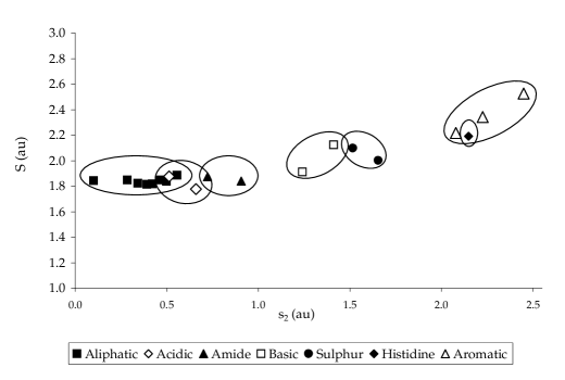
Figure 1: The global softness $S$ of the amino acids as function of the local softness $s_{2}$ of the side-chain, calculated from the SCF density using the 6-311G(d,p) basis set. All values are depicted in au.

Global softness ($S$), local softness of the backbone ($s_{1}$) and side chain ($s_{2}$), global polarizability ($\alpha$) and polarizability of the backbone ($\alpha_{1}$) and side chain ($\alpha_{2}$) of these amino acids are presented in Table 2. Figure 1 depicts the global softness as function of the local softness of the side chain. The linear correlation between these two quantities amounts to $R=0.9242$, while the curve also demonstrates a clear separation of the amino acids into seven reactivity groups recovering to a large extent those defined in Table 1. It must be noted that the hydroxylic amino acids, as well as the proline amino acid, are grouped together with the aliphatic amino acids in the rest of the discussion of the results as the values of their softnesses are overlapping. The values of the local softness $s_{2}$ of the side chains follow the following order: alphatic$<$acidic$<$amide$<$basic$<$sulphur-containing$<$histidine$<$aromatic. At first glance, this order agrees with the chemical intuition. Indeed, one expects the aromatic amino acids, the most polarizable members of the family, to be the “softest”. On the opposite, the aliphatic amino acids, the less polarizable molecules of the family, are expected to be the “hardest”. This reasoning is based on the empirical rule that a polarizable atom is also a soft atom. One will see below that “this rule of thumb” must be used however with care.

Fig. 1 can be compared to Fig. 4 in Ref. References, where the global softness of the amino acids, calculated using the same method and at identical geometries, is depicted as a function of the local softness of the side chain calculated using the method of Contreras et al.[32] Although the values of the local softness of the side chains differ from the values listed in Table 2 in Ref. References, the group separation is completely reproduced using the Hirshfeld-I method, demonstrating the robustness of the softness as a reactivity descriptor and its independence on the details of the partitioning method.

The Coulomb hole and global (average) softness of the backbone fragment $\overline{S}_{1}$ [Eq. (3)], derived by applying a linear regression to the curve $S(s_{2})$ depicted in Fig. 1, are 0.7439 and 1.7113, respectively. Those values differ by only 0.5% from the values listed in Table 1 of Ref. References, being 0.7476 and 1.7196, respectively. The concept of the “Coulomb hole” is thus further confirmed, while its independence on the partitioning method is clearly demonstrated.

On the other hand, the partitioning of amino acids into subgroups observed in Figure 1 and in Ref. (References) can be explained as follows. The global softness $S$ in Table 2 shows relatively little variation among the twenty amino acids, being the smallest for aspartic acid (1.78 au) and largest for tryptophan (2.54 au). On the opposite, the partitioning of the global softness $S$ between the fragments [Eq. (25)] varies considerably. For instance, the local softness of the side chain $s_{2}$ varies between 0.10 au (glycine) and 2.45 (tryptophan). A large similar variation is obviously observed for the softness of the backbone $s_{1}$ as by definition $s_{1}=S-s_{2}$. As shown in Figure 1, points in the (S,s)₂ map which are close identify residues belonging to the same sub-family. The results of Figure 1 can be summarized by saying that “similar molecules have similar global softness and similar contributions of their corresponding fragments to the global softness”.

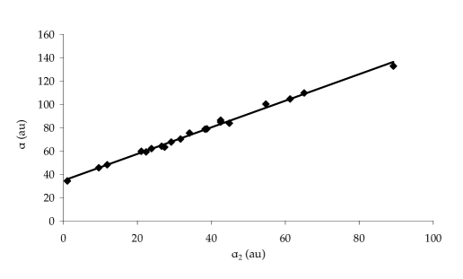
Figure 2: The global polarizability $\alpha$ of the amino acids as function of the local polarizability $\alpha_{2}$ of the side-chain [Eq. (31)], calculated at the MP2/6-311G(d,p) level. All values are depicted in au.

Figure 2 shows the strong correlation ($R=0.9975$) between the global molecular polarizability of an isolated amino acid and the polarizability of its side chain. Therefore the polarizability of an amino acid is largely determined by the polarizability of its side chain. On the other hand, the value of the polarizability of the backbone is similar for all isolated amino acids and has a value close to its average value (28.55$\pm$0.81 au), except for proline (24.75 au) for which the side chain is bounded to the backbone on the contrary to the other amino acids.

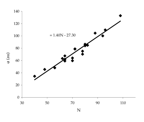
Figure 3: The linear dependence of the polarizabilities of amino acids $\alpha$, calculated at the MP2/6-311G(d,p) level, on the number of electrons $N$.

Another remarkable feature of the polarizability of an isolated amino acid is a strong correlation ($R=0.9659$) between its polarizability and its number of electrons $N$ as can be seen in Figure 3. This correlation is a consequence of the relation between the polarizability and the molecular volume[43]. Indeed, molecular polarizability and molecular volume can be related to each other by using simple electrostatic models. For instance, for a spherical molecule of radius $R$ represented by a dielectric sphere with a macroscopic dielectric constant $\varepsilon,$ the polarizability $\alpha_{sphere}~{}$is given by [44]

$$\alpha_{sphere} = \frac{R^{3}}{4\pi\varepsilon_{0}}\left(\frac{\varepsilon-1}{\varepsilon+1}\right),$$ (48)

$$= \frac{V}{16\pi^{2}\varepsilon_{0}}\left(\frac{\varepsilon-1}{\varepsilon+1}\right),$$ (49)

where $\varepsilon_{0}~{}$is the vacuum permitivity and $V$ the molecular volume. Assuming a homogeneous molecular electronic density,

$$\rho=\frac{N}{V},$$ (50)

one finds

$$\frac{\alpha_{sphere}}{N}=\frac{1}{16\pi^{2}\varepsilon_{0}\rho}\left(\frac{\varepsilon-1}{\varepsilon+1}\right).$$ (51)

In this model, the polarizability per electron would be constant for different molecules of different sizes (measured in the model by the parameter $R$) but having similar properties (controled in the model by the values of the average density $\rho$ and dielectric constant $\varepsilon$). In the case of the amino acids, it must be noted that the approximated linear relation between the molecular size and the molecular polarizability is a consequence of the similarity of the examined molecules, which allows to describe them as a molecular family with $\alpha/N$ varying between 0.85 au (Asp) to 1.2 au (Trp).

Softness and polarizability have always been intuitively related to each other as mentioned above. To test this relation, we have reproduced in Figure 4 the global polarizability per electron global $\alpha/N$ of the amino acids in function of their softness $S$. One observes some qualitative features, for instance, as mentioned above, the aromatic amino acids are the softest and the most polarizable. The correlation coefficient of the linear regression represented in Figure 4 is only $0.7297$. Therefore, one cannot conclude that softness and polarizability are strictly proportional. An example is for instance the couple serine and isoleucine, which have nearly the same softness $S$ $\approx 1.82$ au but different polarizabilities $\alpha/N\approx 0.85$ $[\alpha\approx 48.21]~{}$au for Ser and $\alpha/N\approx 1.1$ $[\alpha\approx 78.65]$ au for Ile.

As was shown in the method section, the lack of proportionality between polarizability and softness is not surprizing since polarizability does not depend directly on the softness but also on the softness dipole vector through the term $\frac{-D^{2}}{3S}$ in Eq. (17). Table 3 lists the $\alpha^{DS}$ contributions to the polarizabilities of the amino acids, their backbones ($\alpha^{DS}_{1}$) and their side chains ($\alpha^{DS}_{2}$), calculated using Eq. 41.

Because the partitioning of the global softness $S$ between the fragments (backbone plus side chain) varies considerably among the amino acids (Table 2), one expects that the dipole-softness polarizability to vary significantly. The dipole-softness polarizability $\alpha^{DS}$ ranges from -0.004 au for aspartic acid to -27.78 au for histidine. The value for histidine is also significantly larger than the rest of the values, the aromatic amino acids having values around -10 au. Also the distribution of the dipole-softness polarizability between the backbone ($\alpha_{1}^{DS}$) and the side chain ($\alpha_{2}^{DS}$) differs from the distribution of the corresponding local softnesses. One observes indeed that local softness values (Table 2) of the side chains ($s_{2}$) increase in the order alphatic$<$acidic$<$amide$<$basic$<$sulphur-containing$<$histidine$<$aromatic, while the values for the backbone ($s_{1}$) decrease in the same order. On the opposite, the variation of the values of the dipole-softness polarizability of the side chains $\alpha_{2}^{DS}$ or of the backbone $\alpha_{1}^{DS}$ of the amino acids (Table 3) does not follow the classification of the residues in the biochemical families. In other words, amino acids with similar $\alpha_{2}^{DS}~{}$ can be in different families as for instance Ala $\alpha_{2}^{DS}=-0.67~{}$ au and Met $\alpha_{2}^{DS}=-0.62$ au. However one observes that absolute large values $|\alpha^{DS}|>2.7$ for aromatic, amide, basic and sulfur-containing amino acids correspond also to large contributions of the side chains $|\alpha^{DS}|\simeq|\alpha_{2}^{DS}|$.

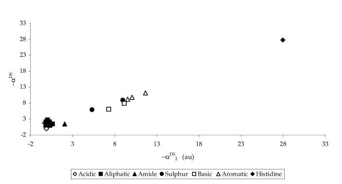
Figure 5: The global dipole-softness polarizability $-\alpha^{DS}$ as function of the the local dipole-softness polarizabilities of the side chain $-\alpha^{DS}_{2}$, calculated from the SCF density obtained with the 6-311G(d,p) basis set. All values are depicted in au.

Figure 5 shows the very good correlation between the dipole-softness polarizability values of the amino acid and those of the side chain, with a correlation coefficient of $R=0.9890$. This plot also allows some separation of the amino acids into reactivity groups, similar to Figure 1, although the order is different showing more overlap. The amino acids are divided into three major groups, the first one containing the acidic, aliphatic and amide amino acids, the second one containing the sulphur-containing, basic and aromatic amino acids and the third group contains histidine, which has a remarkably larger dipole-softness contribution than the rest.

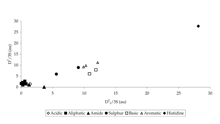
Figure 6: The global dipole-softness polarizability $\frac{D^{2}}{3S}$ as function of the the local dipole-softness polarizabilities of the side chain $\frac{D^{2}_{2}}{3S}$, calculated from the SCF density obtained with the 6-311G(d,p) basis set. All values are depicted in au.

Table 4 contains the dipole-softness contributions partitioned using Eq. (44), where the total contribution to the molecular polarizability $-\frac{D^{2}}{3S}$ is shown (identical to the $\alpha^{DS}$ in Table 3) together with the contribution of the backbone $-\frac{D_{1}^{2}}{3S}$, the side chain $-\frac{D_{2}^{2}}{3S}$ and the interfragmental contribution $-\frac{2\mathbf{D}_{1}\mathbf{D_{2}}}{3S}$. In this partitioning, the dipole-softness polarizabilities of the fragments are negative for the backbone and the side chain, whereas the interfragmental contribution is positive for most amino acids excep Gly and Ala. Remarkably, despite the difference in the two approaches [Eqs. (41) and (44)], the values for the side chains listed in Tables 3 and 4 correlate considerably, with a correlation coefficient of $R=0.9905$. Also the group separation observed in Figure 6 by plotting the dipole-softness polarizabilities as function of $-\frac{D_{2}^{2}}{3S}$, is similar to the one seen in Figure 5, with a slightly lower correlation coefficient of $R=0.9637$. However, the contributions of the backbones, which do not become more negative than -3.2 au in Table 4, do not correlate with the dipole-softness polarizability values of the backbones reported in Table 3. The interfragmental contribution does not reflect the biochemical classification.

One can conclude from Tables 3 and 4 that dipole-softness polarizability is a descriptor which permits to group the amino acids by similarity of their dipole-softness polarizabilities but this classification does not reflect any biochemical classification.

5 Conclusions

The molecular family of amino acids was studied by defining and computing the local softness and the local polarizability of their side chains. The concepts of the local softness of a fragment and of the Coulomb hole of a molecular family, that were introduced in Ref. References, were found independent of the partitioning method of the electronic properties: both the Contreras et al. method (Ref. References) and the Hirshfeld-I method (present work) gave similar results. One concludes that the softness of the side chains allowes to separate the amino acids into groups reflecting their usual biochemical classification. Amino acids within of the same biochemical family are close to each other in the map (S, s₂) (Fig. 1) which means that similar molecules have both similar global and local softnesses.

The polarizability of the twenty amino acids and of their side chains were also computed. The global polarizability was found approximately proportional to the number of electrons $N$ of the amino acid. Indeed, $\alpha/N$ varies between 0.85 au (Asp) to 1.2 au (Trp) within the whole set of amino acids. These results reflect the well-known proportionality between molecular polarizability and molecular size or volume [See Eq. (6)].[43]  Consequently, the polarizability of the side chains does not reflect the biochemical classification of the amino acids on the contrary of their local softness.

The statement that systems which are more polarizable than other are also softer was tested by comparing the softness and polarizability of the side chains of the amino acids. A very moderate correlation was found to exist between global softness and global polarizability per electron. It is shown that the global softness $S$ of two amino acids may be identical whereas their polarizability $\alpha$ differ significantly.

Finaly, a relation was derived between the local polarizability of a molecule and its local softness by applying the Berkowitch-Parr relation. The key quantity is the “softness dipole vector” of a fragment in Eq. (16). We found that the dipole-softness contribution to polarizability exhibits very different behavior than the local softness, explaining the lack of proportionality between softness and polarizability. The softness dipole vector contribution to the polarizability, as well as the polarizability itself, does not reflect the biochemical classification of the amino acids: for example, acidic and amide amino acids have as low values of dipole-softness contribution to the their polarizability as aliphatic amino acids, while histidine has a value of the dipole-softness contribution to the its polarizability almost three times as large as the value for aromatic amino acids.

From the results presented in this paper one can conclude that the often assumed relation between softness and polarizability is not as straightforward as one might think, and that although polarizability and dipole softness undoubtedly reflect somehow the reactivity of a molecule, their values are not good descriptors of the molecular similarity, in contrast to softnesses.

6 Acknowledgments

A.K. and C.V.A. acknowledge the Flemish FWO for research grant nr. G.0629.06. We gratefully acknowledge the University of Antwerp for the access to the university’s CalcUA supercomputer cluster.

7 Tables

Name	Abbrevation	Side Chain	Group
Aspartic Acid	Asp	-ch2cooh	Acidic
Glutamic Acid	Glu	-ch2ch2cooh	Acidic
Alanine	Ala	-ch3	Aliphatic
Glycine	Gly	-h	Aliphatic
Isoleucine	Ile	ch(ch3)ch2ch3	Aliphatic
Leucine	Leu	-ch2ch(ch3)2	Aliphatic
Proline	Pro	-c3h6(ring)	Aliphatic
Serine	Ser	-ch2oh	Hydroxylic
Threonine	Thr	-ch(oh)ch3	Hydroxylic
Valine	Val	-ch(ch3)2	Aliphatic
Asparagine	Asn	-ch2conh2	Amide
Glutamine	Gln	-ch2ch2conh2	Amide
Phenylalanine	Phe	-ch2(phenyl)	Aromatic
Tryptophan	Trp	-ch2(c2h2n)(phenyl)	Aromatic
Tyrosine	Tyr	-ch2(phenyl)oh	Aromatic
Arginine	Arg	-ch2ch2ch2nhc(nh)nh2	Basic
Lysine	Lys	-ch2ch2ch2ch2nh2	Basic
Histidine	His	-ch2c3n2h3(ring)	Histidine
Cysteine	Cys	-ch2sh	Sulphur-containing
Methionine	Met	-ch2ch2sch3	Sulphur-containing

Table 1: The names, abbrevations, and formula’s of the side chain and of the reactivity groups of the twenty amino acids examined in this study.

Name	$S$	s1	s2	$\alpha$	$\alpha_{1}$	$\alpha_{2}$
Asp	1.78	1.12	0.66	59.76	27.99	21.14
Glu	1.88	1.37	0.51	70.38	28.48	31.69
Ala	1.85	1.56	0.29	45.52	29.83	9.55
Gly	1.84	1.74	0.10	34.45	30.46	1.09
Ile	1.82	1.40	0.42	78.65	27.88	38.29
Leu	1.85	1.38	0.46	78.90	28.58	38.82
Pro	1.88	1.33	0.56	63.26	24.75	27.41
Ser	1.82	1.48	0.34	48.21	29.16	11.76
Thr	1.84	1.34	0.50	59.31	27.77	22.41
Val	1.81	1.42	0.39	67.57	27.84	29.20
Asn	1.84	0.94	0.90	64.08	27.93	25.21
Gln	1.87	1.15	0.72	75.27	27.99	34.26
Phe	2.22	0.14	2.08	104.59	28.00	61.31
Trp	2.53	0.08	2.45	132.92	27.76	89.30
Tyr	2.34	0.12	2.23	109.75	28.09	65.17
Arg	2.12	0.71	1.41	100.14	27.74	54.89
Lys	1.91	0.67	1.24	86.51	28.72	42.46
His	2.19	0.04	2.15	84.83	27.35	42.55
Cys	2.00	0.35	1.66	62.03	29.10	23.78
Met	2.10	0.58	1.52	83.96	29.15	44.78

Table 2: Global softness $S$ (Eq. (45)), local softness of the backbone and side chain $s_{1}$ and $s_{2}$ (Eq. (25)), calculated from the SCF density using the 6-311G(d,p) basis set, and global polarizability $\alpha$ and local polarizabilities of the backbone and side chain $\alpha_{1}$ and $\alpha_{2}$ (Eq. (31)) of the twenty amino acids, calculated at the MP2/6-311G(d,p) level of theory. All quantities are in au.

Name	$\alpha^{DS}$	$\alpha^{DS}_{1}$	$\alpha^{DS}_{2}$
Asp	-0.04	-0.15	0.11
Glu	-1.76	-2.05	0.30
Ala	-0.98	-0.67	-0.31
Gly	-1.65	-1.50	-0.16
Ile	-2.69	-2.67	-0.02
Leu	-2.09	-2.24	0.15
Pro	-1.47	-0.86	-0.61
Ser	-2.12	-1.88	-0.25
Thr	-1.51	-1.19	-0.32
Val	-1.99	-1.79	-0.21
Asn	-1.46	0.59	-2.05
Gln	-1.14	-1.38	0.24
Phe	-11.18	0.48	-11.66
Trp	-9.82	0.23	-10.05
Tyr	-9.19	0.35	-9.54
Arg	-6.07	1.22	-7.28
Lys	-7.89	1.25	-9.14
His	-27.78	0.17	-27.95
Cys	-8.91	0.04	-8.96
Met	-5.94	-0.62	-5.31

Table 3: Global dipole-softness polarizability $\alpha^{DS}$, local dipole-softness polarizabilities of the backbone $\alpha^{DS}_{1}$ and side chain $\alpha^{DS}_{2}$ of the twenty amino acids, calculated from the SCF density obtained with the 6-311G(d,p) basis set, using Eq. (41). All quantities are in au.

Name	$-\frac{D^{2}}{3S}$	$-\frac{D^{2}_{1}}{3S}$	$-\frac{D^{2}_{2}}{3S}$	$-\frac{2\mathbf{D}_{1}\mathbf{D}_{2}}{3S}$
Asp	-1.46	-1.68	-1.43	3.07
Glu	-1.76	-3.03	-0.68	1.95
Ala	-0.99	-0.63	-0.27	-0.08
Gly	-1.66	-1.38	-0.04	-0.23
Ile	-2.69	-3.23	-0.59	1.13
Leu	-2.09	-2.97	-0.58	1.46
Pro	-1.47	-1.06	-0.82	0.40
Ser	-2.13	-1.91	-0.29	0.07
Thr	-1.51	-1.44	-0.57	0.49
Val	-1.99	-2.19	-0.61	0.81
Asn	-0.04	-1.00	-3.65	3.19
Gln	-1.14	-2.87	-1.26	2.98
Phe	-11.18	-0.02	-12.16	1.00
Trp	-9.82	-0.01	-10.28	0.47
Tyr	-9.19	-0.02	-9.91	0.73
Arg	-6.07	-2.36	-10.86	7.16
Lys	-7.89	-1.49	-11.88	5.49
His	-27.78	0.00	-28.12	0.34
Cys	-8.91	-0.09	-9.09	0.27
Met	-5.94	-0.92	-5.61	0.60

Table 4: Global dipole-softness polarizability $-\frac{D^{2}}{3S}$, dipole-softness polarizabilities of the backbone $-\frac{D^{2}_{1}}{3S}$, side chain $-\frac{D^{2}_{2}}{3S}$ and the interfragmental contribution $-\frac{2\mathbf{D}_{1}\mathbf{D}_{2}}{3S}$ of the twenty amino acids, calculated from the SCF density obtained with the 6-311G(d,p) basis set using Eq. (44). All quantities are in au.

8 Captions

Figure 1: The global softness $S$ of the amino acids as function of the local softness $s_{2}$ of the side-chain, calculated from the SCF density using the 6-311G(d,p) basis set. All values are depicted in au.

Figure 2: The global polarizability $\alpha$ of the amino acids as function of the local polarizability $\alpha_{2}$ of the side-chain [Eq. (31)], calculated at the MP2/6-311G(d,p) level. All values are depicted in au.

Figure 3: The linear dependence of the polarizabilities of amino acids $\alpha$, calculated at the MP2/6-311G(d,p) level, on the number of electrons $N$.

Figure 4: The polarizability per electron $\alpha/N$, calculated at the MP2/ 6-311G(d,p) level, as function of the global softness $S$ of the amino acids, calculated from the SCF density obtained with the 6-311G(d,p) basis set. All values are depicted in au.

Figure 5: The global dipole-softness polarizability $-\alpha^{DS}$ as function of the the local dipole-softness polarizabilities of the side chain $-\alpha_{2}^{DS}$, calculated from the SCF density obtained with the 6-311G(d,p) basis set. All values are depicted in au.

Figure 6: The global dipole-softness polarizability $\frac{D^{2}}{3S}$ as function of the the local dipole-softness polarizabilities of the side chain $\frac{D_{2}^{2}}{3S}$, calculated from the SCF density obtained with the 6-311G(d,p) basis set. All values are depicted in au.

9 Figures

Figure 4: The polarizability per electron $\alpha/N$, calculated at the MP2/ 6-311G(d,p) level, as function of the global softness $S$ of the amino acids, calculated from the SCF density obtained with the 6-311G(d,p) basis set. All values are depicted in au.

References

- [1] M. Karelson, V. S. Lobanov, and A. R. Katritzky, Chem. Rev. 96, 1027 (1996).
- [2] W. Yang, R. G. Parr, Proc. Natl. Acad. Sci. USA 82, 6723 (1985).
- [3] R. G. Parr, W. Yang, Density-Functional Theory of Atoms and Molecules (New York: Oxford University Press 1989).
- [4] P. Senet, J. Chem. Phys. 105, 6471 (1996).
- [5] P. Geerlings, F. De Proft, Phys. Chem. Chem. Phys. 10, 3028 (2008).
- [6] C. Cardenas, F. De Proft, E. Chamorro, P. Fuentealba, P. Geerlings, J. Chem. Phys 128, 034708 (2008).
- [7] B. S. Kulkarni, A. Tanwar, S. Pal, J. Chem. Sciences 119, 489 (2007).
- [8] K. Hemelsoet, V. Van Speybroeck, M. Waroquier, Chem. Phys. Lett 444, 17 (2007).
- [9] P. W. Ayers, Chem. Phys. Lett. 438, 148 (2007).
- [10] M. H. Cohen, A. Wasserman, J. Phys. Chem. A. 111, 2229 (2007).
- [11] P. Fuentealba, E. Chamorro, C. Cardenas, Int. J. Quant. Chem, 107, 37 (2007).
- [12] R. Kar, K. R. S. Chandrakumar, S. Pal, J. Phys. Chem. A. 111, 375 (2007).
- [13] P. Geerlings, F. De Proft, and W. Langenaeker, Chem. Rev. (Washington, D.C.) 103, 1793 (2003).
- [14] H. Chermette, J. Comput. Chem. 20, 129 (1999).
- [15] Chemical reactivity theory, A Density Functional View, edited by P.K. Chattaraj, CRC Press (2009).
- [16] R. G. Pearson, Proc. Natl. Acad. Sci. U.S.A. 83, 8440 (1986).
- [17] P. Senet, J. Chem. Phys. 107, 2516 (1997).
- [18] P. Senet, Chem. Phys. Lett. 275, 527 (1997).
- [19] W. Yang and W. J. Mortier, J. Am. Chem. Soc. 108, 5708 (1986).
- [20] P. Senet and M. Yang, J. Chem. Sci. 117, 411 (2005).
- [21] P. Senet, F. Aparicio, J. Chem. Phys. 126, 145105 (2007).
- [22] K.E. Laidig and R. F. W. Bader, J. Chem. Phys. 93, 7213(1990).
- [23] F. L. Hirshfeld, Theoret. Chim. Acta (Berl.) 44, 129 (1977).
- [24] J. J. C. Teixeira-Dias and J. N. Murrell, Mol. Phys. 3, 329 (1970).
- [25] K. M. Gough J. Chem. Phys. 91, 2424(1989).
- [26] R. J. W. Le Fevre, Adv. Phys. Org. Chem. 3, 1 (1965).
- [27] K. J. Miller, J. Am. Chem. Soc. 112, 8533 (1990); ibid 8543 (1990).
- [28] B. Rousseau, A. Peeters, C. Van Alsenoy, Chem. Phys. Lett 324, 189 (2000).
- [29] P. Bultinck, C. Van Alsenoy, P. W. Ayers, R. Carbo-Dorca, J. Chem. Phys. 126, 144111 (2007).
- [30] A. Krishtal, P. Senet, M. Yang, C. Van Alsenoy, J. Chem. Phys. 125, 034312 (2006).
- [31] A. Krishtal, P. Senet, C. Van Alsenoy, J. Chem. Theory Comput. 4, 426 (2008).
- [32] R. Contreras, F. Fuentealba, M. Galván, P. Pérez, Chem. Phys. Lett. 304, 405 (1999).
- [33] P. Perez and A. Contreras, Chem. Phys. Lett. 293, 239 1998 .
- [34] J. Melin, F. Aparicio, V. Subramanian, M. Galvan, and P. Chattaraj, J. Phys. Chem. A 108, 2487 2004 .
- [35] Arulmozhiraja, T. Fujii, and G. Sato, Mol. Phys. 100, 423 2002 .
- [36] A. Baeten, F. De Proft, and P. Geerlings, Int. J. Quantum Chem. 60, 931 1996 .
- [37] J. Callaway, Quantum Theory of the Solid State. San Diego: Academic Press 1974.
- [38] G. D. Mahan and K. R. Subbaswamy, Local Density Theory of Polarisability. Springer, 1990.
- [39] M. Berkowitz, R. G. Parr, J. Chem. Phys. 88, 2554 (1988).
- [40] M. J. Frisch, G. W. Trucks, H. B. Schlegel, G. E. Scuseria, M. A. Robb, J. R. Cheeseman, J. A. Montgomery, Jr., T. Vreven, K. N. Kudin, J. C. Burant, J. M. Millam, S. S. Iyengar, J. Tomasi, V. Barone, B. Mennucci, M. Cossi, G. Scalmani, N. Rega, G. A. Petersson, H. Nakatsuji, M. Hada, M. Ehara, K. Toyota, R. Fukuda, J. Hasegawa, M. Ishida, T. Nakajima, Y. Honda, O. Kitao, H. Nakai, M. Klene, X. Li, J. E. Knox, H. P. Hratchian, J. B. Cross, V. Bakken, C. Adamo, J. Jaramillo, R. Gomperts, R. E. Stratmann, O. Yazyev, A. J. Austin, R. Cammi, C. Pomelli, J. W. Ochterski, P. Y. Ayala, K. Morokuma, G. A. Voth, P. Salvador, J. J. Dannenberg, V. G. Zakrzewski, S. Dapprich, A. D. Daniels, M. C. Strain, O. Farkas, D. K. Malick, A. D. Rabuck, K. Raghavachari, J. B. Foresman, J. V. Ortiz, Q. Cui, A. G. Baboul, S. Clifford, J. Cioslowski, B. B. Stefanov, G. Liu, A. Liashenko, P. Piskorz, I. Komaromi, R. L. Martin, D. J. Fox, T. Keith, M. A. Al-Laham, C. Y. Peng, A. Nanayakkara, M. Challacombe, P. M. W. Gill, B. Johnson, W. Chen, M. W. Wong, C. Gonzalez, and J. A. Pople, Gaussian 03, Revision C.02 (Gaussian, Inc., Wallingford CT, 2004)
- [41] C. Van Alsenoy, A. Peeters, J. Mol. Struct (Theochem) 286, 19 (1993).
- [42] T. E. Creighton, Proteins, Structures and Molecular Properties, 2nd ed. Freeman, New York, 1994 .
- [43] T. Brinck, J. S. Murray, P. Politzer, J. Chem. Phys. 98, 4035 (1986) and references therein.
- [44] See e.g., A. Lucas, L. Henrard and Ph. Lambin, Phys. Rev. B 49, 2888 (1994).