Optimal control of magnetization dynamics in ferromagnetic heterostructures by spin-polarized currents

Abstract

We study the switching-process of the magnetization in a ferromagnetic-normal-metal multilayer system by a spin polarized electrical current via the spin transfer torque. We use a spin drift-diffusion equation (SDDE) and the Landau-Lifshitz-Gilbert equation (LLGE) to capture the coupled dynamics of the spin density and the magnetization dynamic of the heterostructure. Deriving a fully analytic solution of the stationary SDDE we obtain an accurate, robust, and fast self-consistent model for the spin-distribution and spin transfer torque inside general ferromagnetic/normal metal heterostructures. Using optimal control theory we explore the switching and back-switching process of the analyzer magnetization in a seven-layer system. Starting from a Gaussian, we identify a unified current pulse profile which accomplishes both processes within a specified switching time.

I Introduction

Spin transfer torque in nanoscaled ferromagnetic/normal–metal (FN) heterostructures has potential application for data storage and manipulation Kisev et al. (2003); Dassow et al. (2005); Pötz et al. (2006). Apart from the experimental studies many theoretical investigations have been made since the pioneering work by Slonczewski and Berger Slonczewski (1996); Berger (1996); Wilczynsky et al. (2008); Alpakov and Visscher (2005); Berkov and Miltat (2008). The problem to describe the physics in FN heterostructures arises from the need to consider the dynamics of the conduction electrons as spin carriers and the dynamics of the localized magnetic moments in parallel and in different regions of the heterostructure. The electron dynamics is faster by several orders of magnitude than that of the latter Zhang and Li (2004). Moreover, the spin dynamics in normal metal regions differs significantly from that in ferromagnetic regions: the former is characterized by fast diffusion and slow spin relaxation, while in the latter the opposite is the case. This time hierarchies make it difficult to provide a fully numerical solution. A Boltzmann–transport theory for magnetic multilayer systems including the spin was developed by Valet–Fert Valet and Fert (1993); Zhang et al. (2004). On the next level of approximation a drift–diffusion equation was applied for mobile spins Barnas et al. (2005). The dynamics of the localized magnetic moments is governed by the Landau–Lifshitz–Gilbert equation (LLGE), extended by additional spin transfer terms. A similar investigation has been performed for semiconductor/ferromagnetic multilayers assuming ballistic transport, but using non–equilibrium Green’s functions Salahuddin and Datta (2006).

In this paper we utilize this time hierarchy and base our model on an exact stationary solution to the spin drift–diffusion equation which we were able to obtain for constant electric current and arbitrary but piece-wise constant layer parameters. We solve self–consistently the LLGE and the spin drift–diffusion equation (SDDE) for the conduction electrons in an external magnetic field to explore switching scenarios as a function of current pulse profiles.

The paper is organized as follows. In Sec. II we present our model for FN multilayer system. Sec. III and Sec. IV are devoted to the mathematical description of the magnetization dynamics (LLGE) and the dynamics of the conduction electrons (SDDE) respectively. The exact solution of our SDDE is given, with details deferred to the Appendix. In Sec. V we present numerical results for a symmetric seven–layer system. Optimal current pulse profiles to switch the magnetization in a given time from parallel to antiparallel state (and in opposite direction) is shown. Our results are compared with our fully numerical simulations to confirm the validity of our approach. Our results regarding critical switching currents versus switching time agree well with earlier work by othersFuchs et al. (2005); Meng et al. (2006) .

II Model

Our model of the heterostructure assumes three different physical building blocks: (i) the normal–metal leads and spacer layers, (ii) ferromagnetic polarizers , and (iii) ferromagnetic analyzers. The leads and the spacer layers are chosen to be nonmagnetic (N) metals with equal material properties. A lead is assumed to be infinitely thick and serving as a spin bath with vanishing spin polarization. We describe a wide ferromagnetic hard polarizer layer ($P_{1}$, $P_{2}$ in Fig. 1) as static and homogeneous. A thin ferromagnetic (soft) analyzer layer (region A in Fig. 1) is treated as a ferromagnetic mono–domain described by a single time–dependent variable, a unit–vector $\textbf{m}(t)$ pointing in the direction of the magnetization Ralph and Stiles (2008); Tserkovnyak et al. (2005). The conduction spin–electrons are treated as classical magnetic moments moving in an external magnetic field created by localized magnetic moments in the ferromagnet. The spin density $\textbf{S}(\textbf{x},t)$ is the dynamical variable to describe the spin distribution Fabian (2007). It is defined for an isolated ferromagnet with magnetization direction m as

$$\textbf{S}=n\mathcal{P}\frac{\hbar}{2}\textbf{m}~{}.$$ (1)

Here $n=n_{\uparrow}+n_{\downarrow}$ is the free electron number density, where $n_{\uparrow,\downarrow}$ is the particle density with spin up/down respectively and $\mathcal{P}=\frac{n_{\uparrow}-n_{\downarrow}}{n}$ corresponds to the spin density polarization, extracted from the experiment Ziese and Thornton (2001). In this work we use for the spin density the dimensionless quantity $\textbf{s}=\textbf{S}/n\frac{\hbar}{2}$. For simplicity we do not consider spin–resolved quantities but use mean values instead (diffusion constant, electric conductivity, spin diffusion length etc.).

III Magnetization dynamics

III.1 Landau-Lifshitz-Gilbert equation

The temporal evolution of the magnetization M is governed by the LLGE Landau and Lifschitz (1975); Ralph and Stiles (2008). Using the saturation magnetization $M_{s}$, we define the quantities $\textbf{M}=M_{s}\textbf{m}$, $\textbf{h}=\gamma\textbf{H}$, where $\gamma$ is the gyromagnetic ratio and $\left(\frac{\partial\textbf{m}}{\partial t}\right)_{st}=\frac{1}{M_{s}}\left(\frac{\partial\textbf{M}}{\partial t}\right)_{st}$ to obtain an equation of motion for the dimensionless magnetization:

$$\frac{d\textbf{m}}{dt}=-\frac{1}{1+\alpha^{2}}\textbf{m}\times\textbf{h}-\frac{\alpha}{1+\alpha^{2}}\textbf{m}\times(\textbf{m}\times\textbf{h})+\left(\frac{\partial\textbf{m}}{\partial t}\right)_{st}~{}.$$ (2)

Here $\textbf{h}=\textbf{h}_{an}+\textbf{h}_{ex}$ is the effective field containing the anisotropy field and external fields measured in units of a frequency and $\alpha$ the Gilbert damping constant. With a unit vector n we set for the anisotropy field

$$\textbf{h}_{an}=\omega_{an}\textbf{n}(\textbf{m}\cdot\textbf{n})~{},$$ (3)

where $\omega_{an}$ is the corresponding frequency. $\left(\frac{\partial\textbf{M}}{\partial t}\right)_{st}$ denotes the spin-transfer term Slonczewski (1996); Berger (1996); Tserkovnyak et al. (2005),

$$\left(\frac{\partial\textbf{m}}{\partial t}\right)_{st}=\xi\textbf{m}\times(\Delta\textbf{I}_{s}\times\textbf{m})~{}.$$ (4)

Here $\Delta\textbf{I}_{s}\equiv(\textbf{I}_{s})_{in}-(\textbf{I}_{s})_{out}$ stands for the spin current absorbed inside the domain, whereas $\xi$ is a constant Stiles and Zangwill (2002); Li and Zhang (2004). Without external torque the equilibrium magnetization is either parallel (P) or antiparallel (AP) to n.

III.2 Dipole field

In this paper we consider the control of the magnetization by spin currents only. So the only contribution to $\textbf{h}_{ex}$ from the outside are the dipole fields originating from the polarizers. In order to obtain a simple result and a crude estimate of the order of magnitude of the dipole fields we consider a polarizer (here written for $P_{1}$ in Fig. 1) as a cylinder with radius $R$ and thickness $x_{1}$ which is homogeneous magnetized and compute the field at the position $x_{m}=(x_{2}+x_{3})/2$. Evaluation of the general integral for a dipole density Jackson (1999) we obtain ($\{\textbf{e}_{x},\textbf{e}_{y},\textbf{e}_{z}\}$ is the canonical basis)

$$\textbf{H}_{d-d}=\frac{1}{4}M_{s}\textbf{e}_{z}~{}\left\{\frac{x_{m}-x_{1}}{\sqrt{R^{2}+(x_{1}-x_{m})^{2}}}-\frac{x_{m}}{\sqrt{R^{2}+x_{m}^{2}}}\right\}.$$ (5)

IV Dynamics of the conduction electrons

A detailed derivation of the balance equation for the spin density $s_{j}(\textbf{x},t)$ is a many particle problem Heide and Zilberman (1999). We use the phenomenological expression for the spin current density Fabian (2007),

$$\textbf{j}_{k}(\textbf{x},t)=-\mu s_{k}(\textbf{x},t)\textbf{E}(t)-D(\textbf{x})\nabla\delta s_{k}(\textbf{x},t)~{}.$$ (6)

$\textbf{j}_{k}$ is the spin current density for electrons with spin–polarization along the $k-$axis. $\mu$ is the electron mobility, which we assume as material–independent, and $\textbf{E}(t)$ is the time–dependent electric field. $D(\textbf{x})$ stands for the material–dependent diffusion constant and $\delta s_{k}(\textbf{x},t)\equiv s_{k}(\textbf{x},t)-s_{k}^{eq}(\textbf{x},t)$ is the non–equilibrium spin density (spin–accumulation), $\textbf{s}^{eq}(\textbf{x},t)$ is the space– and time–dependent equilibrium spin density. We compute the latter using the SDDE, as explained in the next section. Eq. (6) is in general valid for ferromagnetic as well as for nonmagnetic materials. Because of $\nabla\cdot\textbf{E}=0$ inside the metal, we obtain the spin drift–diffusion equation (SDDE) Fabian (2007); Zutic et al. (2002),

$$\frac{\partial\textbf{s}}{\partial t}=\frac{|e|}{m}\textbf{s}\times\textbf{B}+(\nabla D\cdot\nabla)\delta\textbf{s}+D\triangle\delta\textbf{s}+{}$$

$$\mu(\textbf{E}\cdot\nabla)\textbf{s}+\left(\frac{\partial\textbf{s}}{\partial t}\right)_{sf}~{}.$$ (7)

$|e|$ is the elementary charge and $m$ the electron mass ($\mu_{0}$ is the permeability of the vacuum). For the spin flip term we make a spin–relaxation–time ansatz,

$$\left(\frac{\partial\textbf{s}}{\partial t}\right)_{sf}=-\frac{\delta\textbf{s}}{\tau(\textbf{x})}~{},$$ (8)

with the space dependent relaxation time $\tau(\textbf{x})$. For simplicity we assume an isotropic $\tau$ inside each layer. In Eq. (IV) the magnetic induction is related to the magnetization and an external field trough $\textbf{B}(\textbf{x},t)=\mu_{0}(\textbf{H}(\textbf{x},t)+\textbf{M}(\textbf{x},t))$.

IV.1 Spin and charge currents

From now on we will consider quasi–one–dimensional systems along the $x$–axis, such as sketched in Fig. 1. Using Eq. (6) we obtain for the spin current $\textbf{I}_{s}$

$$\textbf{I}_{s}(x,t)=-A\left(\mu E(t)~{}\textbf{s}(x,t)+D(x)~{}\frac{\partial\delta\textbf{s}}{\partial x}(x,t)\right)~{}.$$ (9)

Here $A$ is the cross–section of the sample, and $\textbf{E}(t)=E(t)\textbf{e}_{x}$. In the drift–diffusion model the charge current density is given by Seeger (1973)

$$j(x,t)=n|e|\mu E(t)-D(x)\frac{\partial n}{\partial x}~{}.$$ (10)

We assume homogeneity, $\frac{\partial n}{\partial x}=0$ to obtain

$$j(t)=n|e|\mu E(t)~{}.$$ (11)

A related quantity is the drift–velocity $v_{d}$, used for numerical computations, defined by $v_{d}(t)=-j(t)/n|e|$. For electrons $j$ and $v_{d}$ have opposite sign. $v_{d}>0$, $j<0$ means electrons (spin–carrier) move in the positive $x-$ direction.

IV.2 Equilibrium spin density

Because we consider an arbitrary movement of the analyzer magnetization vector $\textbf{m}(t)$ we have a time–dependent equilibrium spin density (we neglect spin pumping processes induced by moving magnetization Tserkovnyak et al. (2005); Taniguchi and Imamura (2007)). For a fixed time $t$ the equilibrium spin density $\textbf{s}^{eq}(x,t)$ is space–dependent, with a first order approximation (isolated layers),

$$\textbf{s}^{eq}(x,t)\Big{|}_{(1)}\equiv\tilde{\textbf{s}}=\left\{\begin{array}[]{ll}\mathcal{P}\frac{\textbf{B}(t)}{\mid\textbf{B}(t)\mid},&\hbox{$x\in F$;}\\ \textbf{0},&\hbox{$x\in N$.}\\ \end{array}\right.$$ (12)

This expression reflects our choice of dimensionless spin density s in Eq. (6) and Eq. (IV). To obtain the equilibrium spin density in the complete structure we use the general stationary solution Eq. (14) presented in the next section, in which we use the first order expression Eq. (12) for $\textbf{s}^{eq}(x,t)$. We use the boundary conditions for transparent interfaces in F/N–junctions Zutic et al. (2004): $\textbf{s}(x,t)$ and $\textbf{I}_{s}(x,t)$ are continuous. For $E(t)=0$ we obtain in second order $\textbf{s}^{eq}(x,t)\mid_{(2)}$. In the following we omit the subscript $\mid_{(2)}$. Note that, for non–collinear magnetic layers, all components of $\textbf{s}^{eq}(x,t)\neq 0$ in general.

IV.3 Stationary solution of the SDDE for constant parameters

For a given layer, we consider Eq. (IV) for constant current, constant material parameters and time– and space–independent magnetic field. We use $\textbf{s}^{eq}=\tilde{\textbf{s}}$ given by Eq. (12). Setting $\partial\textbf{s}/\partial t=0$ in Eq. (IV), we have for a one dimensional structure the equation

$$D~{}\textbf{s}^{\prime\prime}(x)+\mu E~{}\textbf{s}^{\prime}(x)+\omega~{}\textbf{s}(x)\times\textbf{b}_{1}-\frac{\textbf{s}(x)-\tilde{\textbf{s}}}{\tau}=0~{}.$$ (13)

Here we have defined $\textbf{b}_{1}=\textbf{B}/|\textbf{B}|$, and $\textbf{B}=(m/|e|)\omega\textbf{b}_{1}$, with $\omega$ the Larmor frequency. The general solution of Eq. (13) is a quite lengthy expression, containing 6 integration constants, denoted as $c_{1}\ldots c_{6}$. To find it we split $\textbf{s}(x)$ into two parts, one part parallel to the magnetic field, and the other perpendicular to it,

$$\textbf{s}(x)=\textbf{s}_{\parallel}(x)+\textbf{s}_{\perp}(x)~{}.$$ (14)

We define an orthonormal, positive oriented basis $\{\textbf{b}_{1},\textbf{b}_{2},\textbf{b}_{3}\}$. One finds for the parallel part (where $l_{d}=\mu E\tau$ is the drift length with sign determined by $E$),

$$\textbf{s}_{\parallel}(x)=\textbf{b}_{1}\Bigg{\{}c_{1}\exp\Big{[}-\frac{x[l_{d}+\sqrt{l_{d}^{2}+4\lambda^{2}}]}{2\lambda^{2}}\Big{]}+{}$$

$$c_{2}\exp\Big{[}-\frac{x[l_{d}-\sqrt{l_{d}^{2}+4\lambda^{2}}]}{2\lambda^{2}}\Big{]}\Bigg{\}}+\tilde{\textbf{s}}~{}.$$ (15)

$\textbf{s}_{\parallel}(x)$ does not depend either on $|\textbf{B}(t)|$ or the saturation magnetization. The second part is given by

$$\textbf{s}_{\perp}(x)=\textbf{b}_{2}\Big{\{}c_{3}G_{4}(x)+c_{4}G_{3}(x)+c_{5}G_{2}(x)+{}$$

$$c_{6}G_{1}(x)\Big{\}}+\textbf{b}_{3}\Big{\{}c_{3}G_{3}(x)-c_{4}G_{4}(x)-$$

$$c_{5}G_{1}(x)+c_{6}G_{2}(x)\Big{\}}~{}.$$ (16)

Here the functions $G_{i}(x)$, $i=1,...4$ are given in Appendix A. They depend on the magnetic field and the electric current, not indicated here to simplify the notation. Eq. (14) with Eq. (IV.3) and Eq. (IV.3) present the complete solution of Eq. (13) used in our numerical simulations. We make the following remarks:
(i) The solution of of the SDDE for spin–orientation–dependent material parameters is straightforward.
(ii) Using this solution one can study different boundary conditions when linking layers.
(iii) Because the solutions for spin densities parallel and normal (to the magnetic field) can be separated, it is immediately possible to refine the model using different times $\tau_{1}$ and $\tau_{2}$ for spin relaxation and dephasing.

IV.4 Validity of the quasi–static solution

Here we develop a scheme to estimate the errors from our quasi-static approach. We use the stationary solution from the previous section to compute the spin density for a time–dependent current and magnetization vector. In general this approximation is valid as long as the variation of $j(t)$ and $\textbf{m}(t)$ is slow compared to the shortest relaxation time $\tau$ (quasi–static time–evolution, QSE). A more rigorous estimate of the accuracy of the QSE in comparison with the solution of the full time–dependent equation is a non–trivial task. This is due the different relevant processes and time–scales in the different layers. To get a quantitative picture we set $\textbf{s}(x,t)=\textbf{s}_{qs}(x,t)+\delta\textbf{s}_{qs}(x,t)$, where $\textbf{s}_{qs}(x,t)$ denotes the quasi–static solution Eq. (14) and $\delta\textbf{s}_{qs}(x,t)$ the deviation from the exact solution, denoted as $\textbf{s}(x,t)$. For $\delta\textbf{s}_{qs}(x,t)$ we have inside a single layer the equation

$$\frac{\partial\delta\textbf{s}_{qs}}{\partial t}=\frac{|e|}{m}\delta\textbf{s}_{qs}\times\textbf{B}+D\triangle\delta\textbf{s}_{qs}+{}$$

$$\mu(\textbf{E}\cdot\nabla)\delta\textbf{s}_{qs}-\frac{\delta\textbf{s}_{qs}}{\tau}-\dot{\textbf{s}}_{qs}~{}.$$ (17)

The inhomogeneity is defined as

$$\dot{\textbf{s}}_{qs}:=\frac{\partial\textbf{s}_{qs}}{\partial j}\frac{dj}{dt}+\left(\frac{d\textbf{m}}{dt}\cdot\nabla_{\textbf{m}}\right)\textbf{s}_{qs}~{},$$ (18)

and is the source for a non–vanishing $\delta\textbf{s}_{qs}$. Let us discuss the spin–relaxation in the ferromagnetic layers. Here the typical relaxation time is $\tau\approx 1$ ps and it is reasonable to neglect, in a first approximation, the Larmor, diffusion, and drift terms. The Larmor term is of the order of $1/\omega$, the diffusion is characterized by a time scale $\tau_{d}=l^{2}/D=\tau(l/\lambda)^{2}$, where $l$ is a characteristic finite length (layer thickness). The drift term goes as $\tau_{j}=l/|v_{d}|$. For $l=3$ nm (analyzer thickness as a worst case) this gives $\tau_{d}\approx 0.3\tau$ and $\tau_{j}\approx 0.03$ ns for $j\approx 10^{8}$ A/cm². If we integrate Eq. (IV.4) under this assumptions we find as a first–order correction (for a ferromagnetic layer),

$$\delta\textbf{s}_{qs}^{(1)}(x,t)=-\int_{0}^{t}dt^{\prime}e^{-(t-t^{\prime})/\tau}\dot{\textbf{s}}_{st}(x,t^{\prime})~{}.$$ (19)

If we consider now a spacer layer ($x_{1}\ldots x_{2}$ in Fig. 1) and compare $\tau$ with $\tau_{d}=\tau(l/\lambda)^{2}$ using the parameters given in Tab. I we can see that $\tau_{d}\ll\tau$. Diffusion is dominant in the spacer–layers. It occurs on a time–scale $\tau_{d}\approx 10^{-3}$ ps. In fact, this quite different time–scales in different layers are the reason why an integration of Eq. (IV) by a discretization–procedure used in usual PDE–toolboxes leads to numerical problems. To obtain an estimate of $\delta\textbf{s}_{qs}^{(1)}(x,t)$ inside the spacer–layer we solve Eq. (IV.4) with boundary–conditions given by Eq. (19). Numerical results of this strategy to estimate the accuracy of the QSE will be given below.

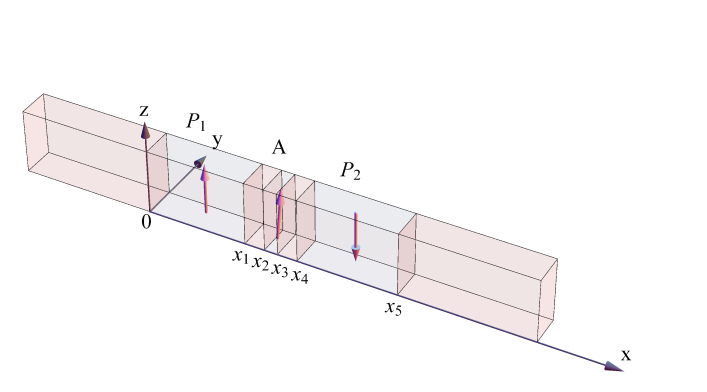
Figure 1: (color online) Geometry of the seven–layer system. The outside layers act as spin–carrier (electron) reservoirs with polarization $\mathcal{P}=0$. The regions $P_{1}$ and $P_{2}$ are the two polarizers, and A is the analyzer layer whose magnetization is to be manipulated.

V Seven–layer system

Fig. 1 shows the seven–layer structure, for which we apply the general formalism. We select this system because such structures where used for low–critical current experiments Fuchs et al. (2005); Meng et al. (2006). This allows testing of the present approach. As indicated in the figure we use two opposite aligned polarizer–layers, polarizer $P_{1}$ points in the $+z$ and polarizer $P_{2}$ in the $-z$ direction. $P_{1}$ defines the parallel position of the analyzer A, where a small deviation from $P_{1}$ is needed for a non–vanishing initial–spin torque. Both polarizers have the same material and geometric properties. As a consequence the dipole field Eq. (5) vanishes exactly at the position of the analyzer A and the anisotropy field Eq. (3) produces two energetically equivalent stable positions (degenerate two–level system). We expect and proof that, if a current pulse $j(t)$ switches the magnetization from P$\rightarrow$AP, then $-j(t)$ does the inverse operation, AP$\rightarrow$P.

V.1 Numerical strategy

All computations are done with the help of Mathematica. We use the solution Eq.(14)-(IV.3) to compute the time– and space–dependent spin density inside of each layer for given direction of B and current $j$. The solution of the total system requires the determination of all integration constants $c_{1}\ldots c_{36}$. Whereas the boundary conditions (continuous spin density and spin current density) are formulated analytically, the solution is computed numerically as a function of m and $j$. The spin current density and the spin torque in Eq. (2) are then calculated self– consistently using Eq.(4). The last step requires the numerical solution of the LLGE, Eq. (2).

V.2 Optimized switching procedure

We now address the switching of the analyzer magnetization (for optimized switching using external magnetic fields see Sun and Wang (2006)). We first note that, due to the non–linearity in m of the LLGE, it is impossible to identify a single current pulse profile which switches both from P$\rightarrow$ AP and AP$\rightarrow$ P (initial–state–independent switching). However, using the symmetry of the structure, one can identify a current pulse profile which, when changing the current direction only, promotes both processes.
To find a simple pulse–shape which performs the desired task it is convenient to use an optimization procedure based on a suitably defined cost–functional $J$ Roloff et al. (2009). We set

$$J=\|\textbf{m}(t_{f})-\textbf{m}_{T}\|~{},\hskip 14.22636pt0\leq J\leq 2~{},$$ (20)

where $\textbf{m}_{T}$ is the target magnetization and $\textbf{m}(t_{f})$ is its actual value at the prescribed target time $t_{f}$. We choose the time–dependent current as

$$j(t;X_{1},X_{2},X_{3})={}$$

$$X_{A}\exp\left\{-\frac{X_{B}}{t_{f}^{2}}(t-t_{f}/2)^{2}\right\}+\sum_{l=1}^{3}X_{l}\sin(l\pi t/t_{f})~{},$$ (21)

with 3 variational parameters $X_{1},\ldots X_{3}$ (one can use also more parameters. Global optimization algorithms however work best with a few parameters). The Gauss–pulse, characterized by $X_{A}$, $X_{B}$, is selected by hand such that it is sufficient to switch the magnetization from P$\rightarrow$AP. It is used as a reference pulse. However, to steer the magnetization in the prescribed time additional current contributions are needed. The additional terms in Eq. (V.2) are constructed to ensure that at the end points of the control–time interval $[0,t_{f}]$ the current vanishes for arbitrary $X_{1,2,3}$. To find the minimum of $J(X_{1},\ldots X_{3})$ a standard line search method or genetic algorithm can be used.

V.3 System–Parameters

We use the material–parameters typical for a Cu_∞ /Fe₁₅/Cu₃/Py₂/Cu₃/Fe₁₅/Cu_∞ (in nm) multilayer–system. The relevant material–parameters are listed in Tab. I Stiles et al. (2004); Reilly et al. (1999); Ziese and Thornton (2001). We use a material–independent electrical conductivity and free–electron–density of $n=84/$nm³.

mat.	$\lambda$  [nm]	$\tau$  [ns]	$M_{s}$  [A/m]	$\omega$ [GHz]	$\mathcal{P}$
Cu	450	0.024	0	0	0
Fe	5	0.001	$17\times 10^{5}$	230	0.45
Py	5	0.001	$8\times 10^{5}$	110	0.37

Table 1: Material–parameters used in the simulation.

We obtain a microscopic expression for the coupling constant $\xi$ given by $\xi=-\frac{|e|n\hbar}{2mM_{s}d}=-0.969/d$, where $d=x_{3}-x_{2}$ is the analyzer thickness. For the Gilbert damping parameter we set $\alpha=0.01$ Fuchs et al. (2007). The direction of the anisotropy field is chosen as $\textbf{n}=(0,\sin(\varphi),-\cos(\varphi))$, with $\varphi=0.9\pi$, and its modulus $\omega_{an}=2$ GHz.

V.4 Results

V.4.1 Switching into constant current

For a first example we consider the dynamics of the seven–layer system in Fig. 1 for a current that we switch on according to $j(t)=j_{0}(1-e^{-t/T})$, with $T=0.5$ ns. We have integrated the LLGE for different values $j_{0}$, as shown in part a) of Fig. 2. Part b) shows the $z-$component of the magnetization as a function of time. In all three cases the magnetization switches from P$\rightarrow$AP, however, the lowest current leads to a switching time of more than 100 ns. These investigations agree well with basic experimental results in the literature Fuchs et al. (2005); Meng et al. (2006): the critical current $|j_{c}|$ is of the order $|j_{c}|\approx 10^{6}$ A/cm², for the parameters chosen here, and depends on the saturation magnetization, Gilbert damping, and anisotropy field Ralph and Stiles (2008). As seen in Fig. 2, switching into a constant spin–polarized current leads to damped oscillations of the magnetization vector. Above the critical current, they result in a flipping of the magnetization vector into the new (AP) equilibrium position. For currents $|j_{0}|<|j_{c}|$ one induces damped oscillations without switching. We should remark that the equilibrium–positions of m for a constant (spin–) current are no more given by the directions of  $\pm\textbf{n}$, but there is small deviation due to the spin current, however, not resolved in Fig. 2.

The seven–layer structure with antiparallel polarizer–orientations is crucial for the occurrence of low $|j_{c}|$. Computations for parallel polarizer orientations ($P_{1}\|P_{2}$) give vastly different critical currents for P$\rightarrow$ AP and AP$\rightarrow$P flips. Fig. 3 reveals the reason for this result. For anti–parallel orientation of the polarizers the $z-$component of the spin density shows a large gradient inside the analyzer layer. As a consequence large spin currents can be generated compared to parallel oriented polarizers. In fact for a simplified model with vanishing dipole field (for sample radius $R\rightarrow\infty$) and parallel polarizers the critical current is $|j_{c}|>10^{8}$ A/cm² for this structure. As investigated, switching times for the analyzer magnetization tend to decrease with increasing $|j_{0}|$ Koch et al. (2004).

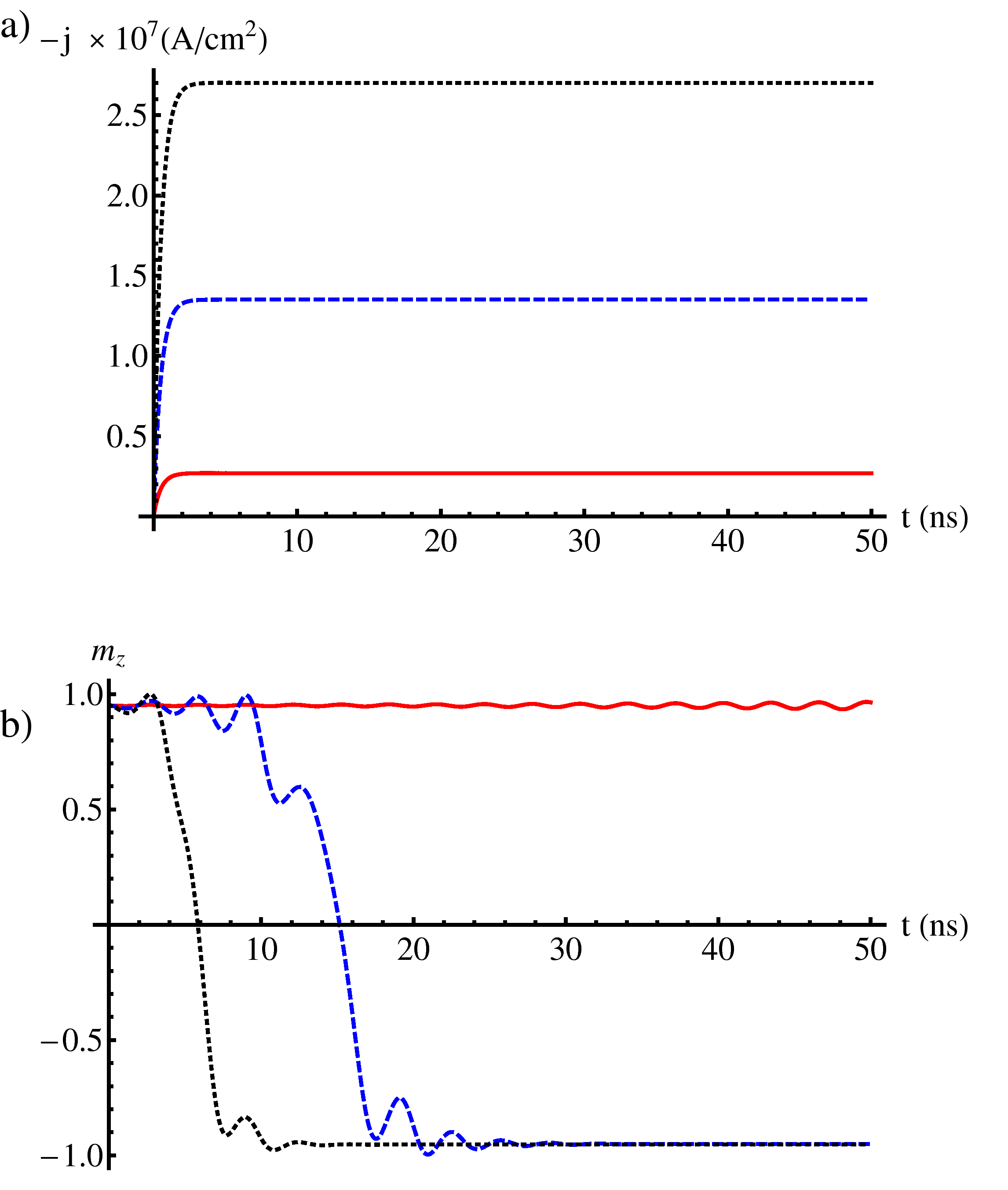
Figure 2: (color online) a) Electric current and b) $z$–component of the magnetization in the analyzer versus time. Associated quantities are plotted in the same line style. For decreasing current the switching time increases. The electric current is plotted as $-j$ according to a positive drift velocity.

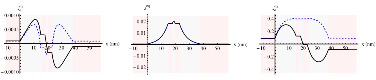
Figure 3: (color online) Equilibrium spin density for two different polarizer alignments. The blue–dashed line corresponds to parallel orientations of the two polarizers, the black–solid line is for anti–parallel orientation, as used in low–current spin–torque experiments. The analyzer is at the position $\textbf{m}=\textbf{n}$ and therefore small perpendicular components of the spin density are present.

V.4.2 Optimal pulse–sequences

We now consider the problem of switching of the magnetization m using an optimized time–dependent electric current, where we set the switching time to $t_{f}=5$ ns. The first current pulse should switch the magnetization from P$\rightarrow$AP. Initial and desired final value of the analyzer magnetization $\textbf{m}(t)$, respectively, are

$$\textbf{m}(0)=\textbf{n}~{}\mbox{and}~{}\textbf{m}(t_{f})\stackrel{{\scriptstyle!}}{{=}}\textbf{m}_{T}=-\textbf{n}~{}.$$ (22)

A numerical minimization of Eq. (20), limiting ourselves to the pulse shape Eq. V.2, gives as a result the first pulse shown in Fig. 5. We stopped the computation when the cost functional was $J\approx 0.006$. This means that the optimal control pulse, rather than relying on intrinsic Gilbert damping, actively drives the magnetization precisely into the target state AP; likewise for the back flip, see Fig. 5 (c). Note that the pulse shape is chosen such that the current is zero at the boundaries of the time interval. To ensure that the magnetization remains in the AP state after the first flip, a few ns later we apply the same pulse once more. Only a weak deviation from the equilibrium position in form of a few damped oscillations are visible demonstrating stability, see Fig. 5. However when we apply the same pulse profile with opposite current direction we switch the magnetization back from AP$\rightarrow$P. In addition to $\textbf{m}(t)$ we have plotted in Fig. 5 the time–dependent spin density during the first current pulse. The rows (a) and (b), respectively, show the equilibrium spin density and its deviation from equilibrium inside the multilayer device. One observes the degree to which the equilibrium spin density depends on the time–dependent magnetization $\textbf{m}(t)$: due to the choice of the magnetization of $P_{1}$ and $P_{2}$ (as collinear) only the $z$–component of the spin density shows significant deviation from equilibrium. The order of magnitude of the deviation of $x$– and $y$–components is of the order of the error made by the QSE. The non–equilibrium spin density as function of time is influenced by the actual position of $\textbf{m}(t)$ and the current $j(t)$, as well as the magnetization of $P_{1}$ and $P_{2}$ .

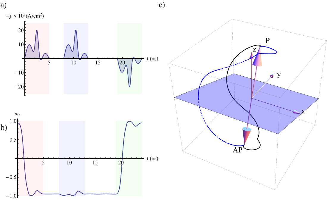
Figure 4: (color online) a) Optimized time–dependent electric current for switching the analyzer magnetization from P$\rightarrow$AP and vice versa. Three 5 ns pulses with the same shape are applied. The first switches from P$\rightarrow$AP, the second is used to test stability, and the third switches back AP$\rightarrow$P. b) $z$–component of the analyzer magnetization vector $\textbf{m}(t)$ as a function of time. c) Plot of the three–dimensional trajectory of $\textbf{m}(t)$ during the first (black, solid) and last pulse (blue, dashed).

V.4.3 Error estimate

We have used the results from the previous section to test the numerical validity of the stationary solution as discussed in Sec. IV.4. Fig. 6 shows the estimate for the deviation of the $z-$ component of the spin density in selected parts of the structure. The solid line is for the center of $P_{1}$, while the dashed line is for the center of the spacer layer to the left of the analyzer. The figure shows that $[\delta\textbf{s}_{qs}^{(1)}]_{z}$, depending on position, is of the order of $10^{-5}-10^{-4}$, compared with $s_{z}^{eq}\approx 0.1-0.3$ (see Fig. 3). The dominant contribution in Eq. (18) comes from the moving magnetization, whereas the current contribution is neglibile. For the other components we obtained similar results regarding relative errors.

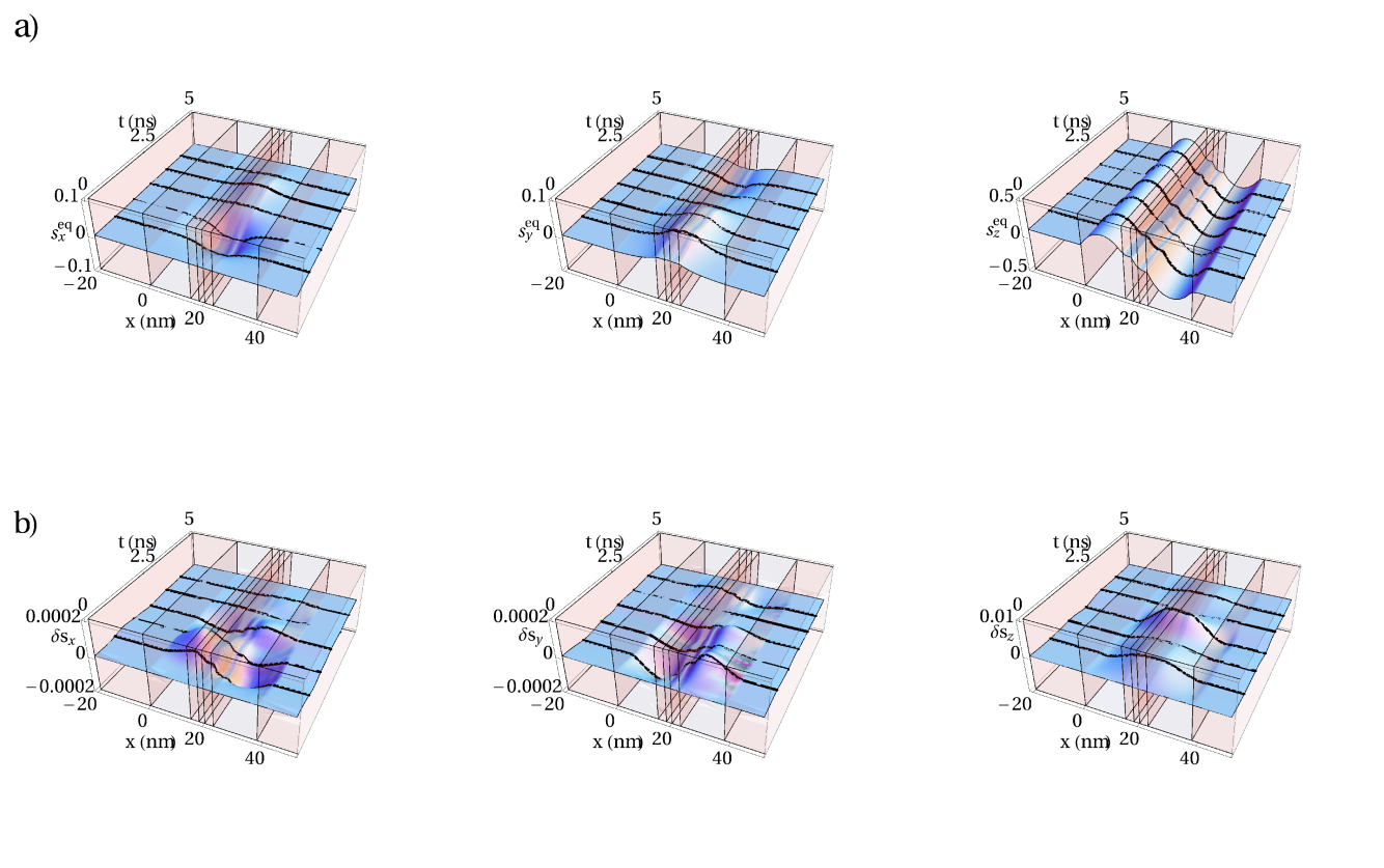
Figure 5: (color online) a) The first row shows the equilibrium spin density for the switching process P$\rightarrow$ AP for the first pulse in Fig. 4. It depends on $\textbf{m}(t)$. b) Non–equilibrium spin density induced by the electrical–current pulse. The computed values for $\delta s_{x}$, $\delta s_{y}$, however, are at the limit of the accuracy of the QSE.

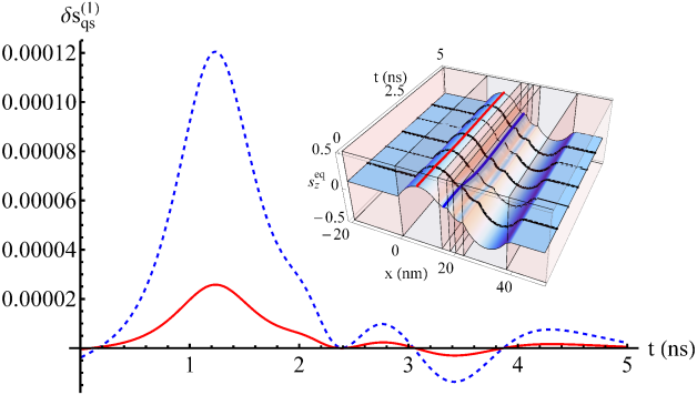
Figure 6: (color online) Numerical estimate of the error within the QSE relative to an exact treatment of the SDDE. The inset shows the locations where we compute $\delta\textbf{s}_{qs}^{(1)}$. Inside the polarizer (red–solid line) we use Eq. (19) to estimate the deviation from the exact result, whereas inside the spacer–layer, Eq. (IV.4) is integrated numerically.

VI Conclusions and outlook

We have presented a self–consistent model for magnetization switching by spin–polarized electric current in metallic ferromagnetic heterostructures. Our method is founded upon an analytic solution of the stationary spin drift–diffusion equation (SDDE) for each layer using constant material parameters, electric current, and magnetic field. Matching layers, using continuity of spin density and spin current density at the interfaces as boundary conditions, we obtain an analytic solution for the spin density of the entire heterostructure. Making a quasi–static approximation in which the time dependence of the spin density depends on time solely via the electric current and net magnetic field, the time evolution of the spin density is computed in parallel to the Landau–Lifshitz–Gilbert (LLGE) equation. Both equations couple via the spin torque effect and the time–dependent magnetization in the SDDE. This method allows for an efficient and robust mathematical description of the coupled carrier spin and magnetization dynamics in metal/ferromagnet heterostructures. Because the model is based on a completely analytic solution of the stationary SDDE for given electric current and magnetic field for each layer, it is applicable to heterostructures of high complexity, for example for tilted polarizers or structures exposed to external magnetic fields He et al. (2010).
We have demonstrated the efficiency of this semi–analytic approach by investigating a seven–layer system with antiparallel oriented polarizers, as studied in recent experiments, and computed optimized current pulses to switch the magnetization from P$\rightarrow$AP$\rightarrow$P in specified time of 5 ns. As expected for the system under investigation, the obtained current densities are in the range of $10^{8}$ A/cm², with a critical current of about $10^{6}$ A/cm². Using optimal control theory, we identify solutions for current profiles which allow for precise switching in predetermined switching times. We provide and discuss one example.
Furthermore, a detailed investigation of the validity of the quasi–static time evolution of the SDDE is given. It confirms excellent accuracy for the example of the simulated seven–layer heterostructure.
Several future applications of the presented formalism can be envisioned. A combined variation of material– and geometric parameters to obtain optimal current pulses with low critical currents. A description of thermal fluctuations using temperature–dependent effective (Langevin–) fields in the LLGE (via the spin torque in the SDDE) and the search of ”thermally robust” current pulses by averaging over many field configurations.

Appendix A Stationary solution of the SDDE

Here we summarize the remaining analytic expressions for the stationary solution and constant material parameters as presented in Sec. IV.3. We use the dimensionless quantities $\kappa:=\omega\tau$ and $\rho:=l_{d}/\lambda$. Further we define

$$a=\mathrm{Re}[\sqrt{4+\rho^{2}+4i\kappa}]={}$$

$$\sqrt{\frac{4+\rho^{2}}{8}+\sqrt{\frac{\kappa}{2}\left[1+\left(\frac{4+\rho^{2}}{4\kappa}\right)^{2}\right]}}~{},$$ (23)

$$b=\mathrm{Im}[\sqrt{4+\rho^{2}+4i\kappa}]={}$$

$$\sqrt{-\frac{4+\rho^{2}}{8}+\sqrt{\frac{\kappa}{2}\left[1+\left(\frac{4+\rho^{2}}{4\kappa}\right)^{2}\right]}}~{}.$$ (24)

Using the auxiliary functions,

$$F_{1}(x)=e^{-\frac{\rho x}{2\lambda}}\cos\left(\frac{bx}{2\lambda}\right)\sinh\left(\frac{ax}{2\lambda}\right)~{},$$ (25)

$$F_{2}(x)=e^{-\frac{\rho x}{2\lambda}}\cosh\left(\frac{ax}{2\lambda}\right)\sin\left(\frac{bx}{2\lambda}\right)~{},$$ (26)

$$F_{3}(x)=e^{-\frac{\rho x}{2\lambda}}\cos\left(\frac{bx}{2\lambda}\right)\cosh\left(\frac{ax}{2\lambda}\right)~{},$$ (27)

$$F_{4}(x)=e^{-\frac{\rho x}{2\lambda}}\sin\left(\frac{bx}{2\lambda}\right)\sinh\left(\frac{ax}{2\lambda}\right)~{},$$ (28)

the four dimensionless functions $G_{i}(x)$, entering in Eq. (IV.3) are:

$$G_{1}(x)=\left[-4a^{3}\rho\kappa+4a\rho\kappa(4+3b^{2}+\rho^{2})\right]F_{1}(x)+{}$$

$$\left[4b^{3}\rho\kappa+4b\rho\kappa(4-3a^{2}+\rho^{2})\right]F_{2}(x)-{}$$

$$4\kappa(a^{2}+b^{2})(-4+a^{2}-b^{2}-\rho^{2})F_{3}(x)-{}$$

$$8ab(a^{2}+b^{2})\kappa F_{4}(x)~{},$$ (29)

$$G_{2}(x)=a\rho\left[a^{4}+(4+5b^{2}+\rho^{2})(4-2a^{2}+b^{2}+\rho^{2})\right]F_{1}(x)+{}$$

$$b\rho\left[5a^{4}+(4+b^{2}+\rho^{2})^{2}-2a^{2}(12+5b^{2}+3\rho^{2})\right]F_{2}(x)-{}$$

$$(a^{2}-b^{2})\left[(a^{2}+b^{2}-\rho^{2}-4)^{2}-4a^{2}b^{2}\right]F_{3}(x)+{}$$

$$4ab(a^{2}-b^{2})\kappa\left[4-a^{2}+b^{2}+\rho^{2}\right]F_{4}(x)~{},$$ (30)

$$G_{3}(x)=\left[24a^{2}b\kappa-8b\kappa(4+b^{2}+\rho^{2})\right]F_{1}(x)+{}$$

$$\left[24ab^{2}\kappa+8a\kappa(4-a^{2}+\rho^{2})\right]F_{2}(x)~{},$$ (31)

$$G_{4}(x)=\left[-8a^{3}\kappa+8a\kappa(4+3b^{2}+\rho^{2})\right]F_{1}(x)+{}$$

$$\left[8b^{3}\kappa+8b\kappa(4-3a^{2}+\rho^{2})\right]F_{2}(x)~{}.$$ (32)

The integration of the normal component of Eq. (13) requires the solution of two second order differential equations. It is advantageous to transform this two second order equations into four first order equations and solve this system by matrix exponentiation. This procedure, after some simplifications, leads to the four functions $G_{i}(x)$, which build the fundamental solution.

References

- Kisev et al. (2003) S. I. Kisev, J. Sankey, I. Krirovotov, N. Emley, R. Schoelkopf, R. Buhrman, and D. Ralph, Nature 425, 380–382 (2003).
- Dassow et al. (2005) H. Dassow, R. Lehndorff, D. Bürgler, M. Buchmeier, P. Grünberg, C. Schneider, and A. van der Hart., IFF Scientific Report 2004/2005 (2005).
- Pötz et al. (2006) W. Pötz, J. Fabian, and U. Hohenester, Modern aspects of spin physics (Lecture notes in physics) (Springer–Verlag Wien NewYork, 2006).
- Slonczewski (1996) J. Slonczewski, Journal of Magnetism and Magnetic Materials 159 L1–L7 (1996).
- Berger (1996) L. Berger, Phys. Rev. B 54, 9353–9358 (1996).
- Wilczynsky et al. (2008) M. Wilczynsky, J. Barnas, and R. Swirkovicz, Phys. Rev. B 77, 054434 (2008).
- Alpakov and Visscher (2005) D. M. Alpakov and P. B. Visscher, Phys. Rev. B 72, 180405 (R) (2005).
- Berkov and Miltat (2008) D. V. Berkov and J. Miltat, Journal of Magnetism and Magnetic Materials 320 1238–1259 (2008).
- Zhang and Li (2004) S. Zhang and Z. Li, Phys. Rev. Lett. 93, 12 (2004).
- Valet and Fert (1993) T. Valet and A. Fert, Phys. Rev. B 48, 10 (1993).
- Zhang et al. (2004) J. Zhang, P. M. Levy, S. Zhang, and V. Antropov, Phys. Rev. Lett. 93, 256602 (2004).
- Barnas et al. (2005) J. Barnas, A. Fert, M. Gmitra, I. Weymann, and V. K. Dugaev, Phys. Rev. B 72, 024426 (2005).
- Salahuddin and Datta (2006) S. Salahuddin and S. Datta, Appl. Phys. Lett. 89, 153504 (2006).
- Fuchs et al. (2005) G. Fuchs, I. Krivotorov, P. Braganca, N. Emley, A. Garcia, D. Ralph, and R. Buhrman, Appl. Phys. Lett. 86, 152509 (2005).
- Meng et al. (2006) H. Meng, J. Wang, and J.-P. Wang, Appl. Phys. Lett. 88, 082504 (2006).
- Ralph and Stiles (2008) D. C. Ralph and M. D. Stiles, Journal of Magnetism and Magnetic Materials 320 1190–1216 (2008).
- Tserkovnyak et al. (2005) Y. Tserkovnyak, A. Brataas, G. E. W. Bauer, and B. I. Halperin, Rev. Mod. Phys. Vol. 77, No. 4 (2005).
- Fabian (2007) J. Fabian, Acta Physica Slovaca Vol. 57, No. 4&5, 565–907 (2007).
- Ziese and Thornton (2001) M. Ziese and M. J. Thornton, Spin Electronics (Lecture notes in physics (Springer–Verlag Wien NewYork, 2001).
- Landau and Lifschitz (1975) L. D. Landau and E. M. Lifschitz, Lehrbuch der theoretischen Physik, IX, Statistische Physik, Teil 2 (Akademie Verlag Berlin, 1975).
- Stiles and Zangwill (2002) M. D. Stiles and A. Zangwill, Phys. Rev. B 66, 014407 (2002).
- Li and Zhang (2004) Z. Li and S. Zhang, Phys. Rev. B 70, 024417 (2004).
- Jackson (1999) J. D. Jackson, Classical Electrodynamics (third edit.) (John Wiley and sons, inc, 1999).
- Heide and Zilberman (1999) C. Heide and P. E. Zilberman, Phys. Rev. B 60, 21 (1999).
- Zutic et al. (2002) I. Zutic, J. Fabian, and S. D. Sarma, Phys. Rev. Lett. 88, 6 (2002).
- Seeger (1973) K. Seeger, Semiconductor Physics (Springer–Verlag Wien NewYork, 1973).
- Taniguchi and Imamura (2007) T. Taniguchi and H. Imamura, Phys. Rev. B 76, 092402 (2007).
- Zutic et al. (2004) I. Zutic, J. Fabian, and S. D. Sarma, Rev. Mod. Phys. Vol. 76, No. 2 (2004).
- Sun and Wang (2006) Z. Z. Sun and X. R. Wang, Phys. Rev. Lett. 97, 077205 (2006).
- Roloff et al. (2009) R. Roloff, M. Wenin, and W. Pötz, Journal of Computational and Theoretical Nanoscience, Vol. 6, Nr. 8,1837–1863 (2009).
- Stiles et al. (2004) M. D. Stiles, J. Xiao, and A. Zangwill, Phys. Rev. B 69, 054408 (2004).
- Reilly et al. (1999) A. Reilly, W. Park, R. Slater, B. Ouaglal, R. Loloee, W. Pratt, and J. Bass, Journal of Magnetism and Magnetic Materials 195 (1999).
- Fuchs et al. (2007) G. Fuchs, J. Sankey, V. Pribiag, L. Qian, P. Braganca, A. Garcia, E. Ryan, Z. Li, O. Ozatay, D. Ralph, et al., Appl. Phys. Lett. 91, 062507 (2007).
- Koch et al. (2004) R. H. Koch, J. A. Katine, and J. Z. Sun, Phys. Rev. Lett. 92, 8 (2004).
- He et al. (2010) P. He, R. X. Wang, Z. D. Li, Q. Liu, A. Lan, Y. G. Wang, and B. S. Zou, Eur. Phys. J. B 73, 417–421 (2010).