Drawing Trees with Perfect Angular Resolution
and Polynomial Area

Abstract

We study methods for drawing trees with perfect angular resolution, i.e., with angles at each node $v$ equal to $2\pi/d(v)$. We show:

1. Any unordered tree has a crossing-free straight-line drawing with perfect angular resolution and polynomial area.

2. There are ordered trees that require exponential area for any crossing-free straight-line drawing having perfect angular resolution.

3. Any ordered tree has a crossing-free Lombardi-style drawing (where each edge is represented by a circular arc) with perfect angular resolution and polynomial area.

Thus, our results explore what is achievable with straight-line drawings and what more is achievable with Lombardi-style drawings, with respect to drawings of trees with perfect angular resolution.

1 Introduction

Most methods for visualizing trees aim to produce drawings that meet as many of the following aesthetic constraints as possible:

• straight-line edges,

• crossing-free edges,

• polynomial area, and

• perfect angular resolution around each node.

These constraints are all well-motivated, in that we desire edges that are easy to follow, do not confuse viewers with edge crossings, are drawable using limited real estate, and avoid congested incidences at nodes. Nevertheless, previous tree drawing algorithms have made various compromises with respect to this set of constraints; we are not aware of any previous tree-drawing algorithm that can achieve all these goals simultaneously. Our goal in this paper is to show what is actually possible with respect to this set of constraints and to expand it further with a richer notion of edges that are easy to follow. In particular, we desire tree-drawing algorithms that satisfy all of these constraints simultaneously. If this is provably not possible, we desire an augmentation that avoids compromise and instead meets the spirit of all of these goals in a new way, which, in the case of this paper, is inspired by the work of artist Mark Lombardi [23].

Problem Statement.

The art of Mark Lombardi involves drawings of social networks, typically using circular arcs and good angular resolution. Figure 1 shows such a work of Lombardi that is crossing-free and almost a tree. It makes use of both circular arcs and straight-line edges. Inspired by this work, let us define a set of problems that explore what is achievable for drawings of trees with respect to the constraints listed above but that, like Lombardi’s drawings, also allow curved as well as straight-line edges.

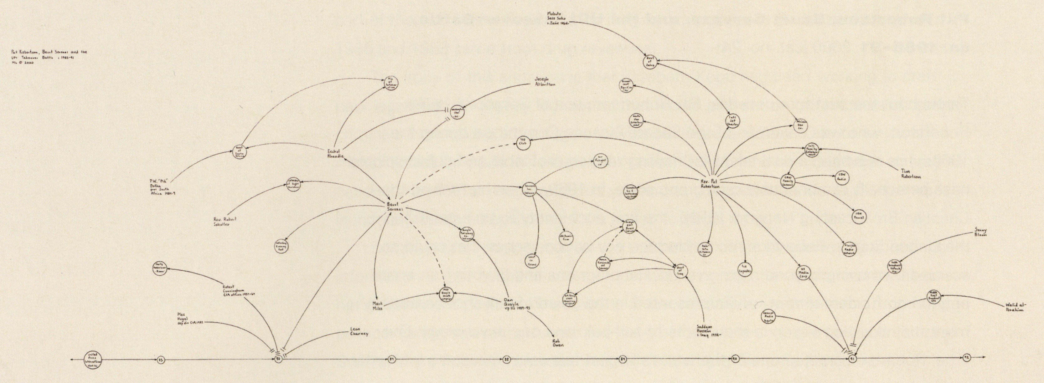
Figure 1: Pat Robertson, Beurt Servaas and the UPI Takeover Battle, ca. 1985-91. Drawing by Mark Lombardi, 2000. Image courtesy of Pierogi.

A drawing of a graph $G=(V,E)$ is an assignment of a unique point in the Euclidean plane to each node in $V$ and an assignment of a simple curve to each edge $(u,v)\in E$ such that the only two nodes in $V$ intersected by the curve are $u$ and $v$, which coincide with the endpoints of the curve. A drawing is straight-line if every edge is drawn as a straight-line segment. A drawing is planar if no two curves intersect except at a common shared endpoint.

Given a graph $G=(V,E)$, let $d(u)$ denote the degree of a node $u$, i.e., the number of edges incident to $u$ in $G$. For a drawing of $G$, the angular resolution at a node $u$ is the minimum angle between any two edges incident to $u$. A node has perfect angular resolution if its angular resolution is ${2\pi}/{d(u)}$, and a drawing has perfect angular resolution if every node does.

Suppose that our input graph $G$ is a rooted tree $T$. We say that $T$ is ordered if an ordering of the edges incident to each node in $T$ is specified. Otherwise, $T$ is unordered.

In many drawings of graphs, nodes can be placed on an integer grid, allowing one to get a bound on the area of the drawing by bounding the dimensions of the grid. Drawings with perfect angular resolution cannot be placed on an integer grid unless the degrees of the nodes are constrained. To see this, suppose we have a vertex $u$ and two of its (consecutive) neighbors all of which lie on Cartesian grid points. From basic trigonometry, the area of the triangle defined by these points is $\frac{1}{2}ab\sin{\theta}$, where $a$ and $b$ represent the lengths of the edges extending from $u$ and $\theta=2\pi/d(u)$ is the angle between these two edges. By Pick’s theorem, the area of this triangle is rational, and consequently so is the square of the area. Since $a^{2}$ and $b^{2}$ must also be rational, we conclude that $\sin^{2}{\theta}$ must be rational. This is false for nearly all values of $d(u)$, for example, when $d(u)=10$ and $\theta=\pi/5$. Hence, if we wish to have perfect angular resolution, we cannot require the nodes to have integer coordinates.

In this paper, our focus is on producing planar drawings of trees with perfect angular resolution in polynomial area. When defining the area of a drawing, it is important that the area measure prevents the drawing from being arbitrarily scaled down. Our algorithms achieve polynomial area bounds according to the following three typical area measures for non-grid drawings. In the first measure, the area is defined as the ratio of the area of a smallest disk enclosing the drawing to the square of the length of its shortest edge. As two non-neighboring nodes can be arbitrarily close using this definition, one may be interested in using another definition of area instead, the (squared) ratio of the farthest pair of nodes to the closest pair of nodes in the drawing. This area measure can also be defined in terms of edges instead of nodes, i.e., as the (squared) ratio of the farthest pair of edges to the closest pair of non-adjacent edges.

We define a Lombardi drawing [11] of a graph $G$ as a drawing of $G$ with perfect angular resolution such that each edge is drawn as a circular arc. When measuring the angle formed by two circular arcs incident to a node $v$, we use the angle formed by the tangents of the two arcs at $v$. Circular arcs are strictly more general than straight-line segments, since straight-line segments can be viewed as circular arcs with infinite radius. Figure 2 shows an example of a straight-line drawing and a Lombardi drawing for the same tree. Thus, we can define our problems as follows:

1. Is it always possible to produce a straight-line drawing of an unordered tree with perfect angular resolution and polynomial area?

2. Is it always possible to produce a straight-line drawing of an ordered tree with perfect angular resolution and polynomial area?

3. Is it always possible to produce a Lombardi drawing of an ordered tree with perfect angular resolution and polynomial area?

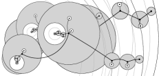
(a) Straight-line drawing for an unordered tree

(b) Lombardi drawing for an ordered tree

Figure 2: Two drawings of a tree $T$ with perfect angular resolution and polynomial area as produced by our algorithms. Bold edges are heavy edges, gray disks are heavy nodes, and white disks are light children. The root of $T$ is in the center of the leftmost disk.

Related Work.

Tree drawings have interested researchers for many decades: e.g., hierarchical drawings of binary trees date to the 1970’s [31]. Many improvements have been proposed since this early work, using space efficiently and generalizing to non-binary trees[2, 5, 17, 18, 19, 28, 29, 30]. These drawings fail to meet the four constraints mentioned earlier, especially the constraint on angular resolution.

Several other methods directly aim to optimize angular resolution in tree drawings. Radial drawings of trees place nodes at the same distance from the root on a circle around the root node [12]. Circular tree drawings are made of recursive radial-type layouts [26]. Bubble drawings [20] draw trees recursively with each subtree contained within a circle disjoint from its siblings but within the circle of its parent. Balloon drawings [24] take a similar approach and heuristically attempt to optimize space utilization and the ratio between the longest and shortest edges in the tree. Convex drawings [4] partition the plane into unbounded convex polygons with their boundaries formed by tree edges. Although these methods provide several benefits, none of these methods guarantees that they satisfy all of the aforementioned constraints.

The notion of drawing graphs with edges that are circular arcs or other nonlinear curves is certainly not new to graph drawing. For instance, Cheng et al. [6] use circular arcs to draw planar graphs in an $O(n)\times O(n)$ grid while maintaining bounded (but not perfect) angular resolution. Similarly, Dickerson et al. [7] use circular-arc polylines to produce planar confluent drawings of non-planar graphs, Duncan et al. [8] draw graphs with fat edges that include circular arcs, and Cappos et al. [3] study simultaneous embeddings of planar graphs using circular arcs. Finkel and Tamassia [15] use a force-directed method for producing curvilinear drawings, and Brandes and Wagner [1] use energy minimization methods to place Bézier splines that represent connections in a train network.

In a separate paper [11] we study Lombardi drawings for classes of graphs other than trees. Unlike trees, not all planar graphs have planar Lombardi drawings [11, 9] and it is an interesting open question to characterize the graphs that have a planar Lombardi drawing. Eppstein [14] recently proved that all planar subcubic graphs have a planar Lombardi drawing, and that there are 4-regular planar graphs that do not have a planar Lombardi drawing. He also characterized the planar graphs that have planar Lombardi drawings corresponding to physical soap bubble clusters [13]. Löffler and Nöllenburg [25] showed that all outerpaths, i.e., outerplanar graphs whose weak dual is a path, have an outerplanar Lombardi drawing. In terms of the usability of Lombardi drawings, two independent user studies [27, 32] examined the performance of Lombardi versus straight-line drawings for several graph reading tasks. While the study of Purchase et al. [27] showed an advantage of straight-line drawings for two out of three tasks, but aesthetic preference for Lombardi drawings, the study of Xu et al. [32] did not show significant performance differences between the two types of drawings, but a strong aesthetic preference for straight-line drawings.

Our Contributions.

In this paper we present the first algorithm for producing straight-line, crossing-free drawings of unordered trees that ensures perfect angular resolution and polynomial area. In addition we show, in Section 3, that if the tree is ordered then it is not always possible to maintain perfect angular resolution and polynomial drawing area when using straight lines for edges. Nevertheless, in Section 4, we show that crossing-free polynomial-area Lombardi drawings of ordered trees are possible. That is, we show that the answers to the questions posed above are “yes,” “no,” and “yes,” respectively. Both algorithms require linear time in a model of computation, in which we can perform trigonometric computations and find roots of bounded degree polynomials in constant time.

2 Straight-line drawings for unordered trees

Let $T$ be an unordered tree with $n$ nodes. We wish to construct a straight-line drawing of $T$ with perfect angular resolution and polynomial area.

The main idea of our algorithm is, similarly to the common bubble and balloon tree constructions [20, 24], to draw the children of each node of the given tree in a disk centered at that node; however, our algorithm differs in several key respects in order to achieve the desired area bounds and perfect angular resolution.

2.1 Heavy Path Decomposition

The initial step before drawing the tree $T$ is to create a heavy path decomposition [22] of $T$. To make the analysis simpler, we assume $T$ is rooted at some arbitrary node $r$. We let $T_{u}$ represent the subtree of $T$ rooted at $u$, and $|T_{u}|$ the number of nodes in $T_{u}$. A node $c$ is the heavy child of $u$ if $|T_{c}|\geq|T_{v}|$ for all children $v$ of $u$. In the case of a tie, we arbitrarily designate one node as the heavy child. We refer to the non-heavy children as light and let $L(u)$ denote the set of all light children of $u$. The light subtrees of $u$ are the subtrees of all light children of $u$. We define $l(u)=1+\sum_{v\in L(u)}|T_{v}|$ to be the light size of $u$. An edge is called a heavy edge if it connects a heavy child to its parent; otherwise it is a light edge. The set of all heavy edges creates the heavy-path decomposition of $T$, a disjoint set of (heavy) paths where every node in $T$ belongs to exactly one path (possibly of length 0); see Figure 3. After an initial bottom-up traversal of $T$ to compute the number of descendants for every node, the heavy-path decomposition can be computed by a depth-first search that always descends to the heavy child of each node before visiting its light children in arbitrary order. This takes $O(n)$ time.

The heavy path decomposition has the following important property. If we treat each heavy path as a node, and each light edge as connecting two heavy-path nodes, we obtain a tree $H(T)$. This tree has height $h(T)\leq\log_{2}{n}$ since the size of each light child is less than half the size of its parent. We refer to the level of a heavy path as the depth of the corresponding node in the decomposition tree, where the root has depth 0. We extend this notion to nodes, i.e., the level of a node $v$ is the level of the heavy path to which $v$ belongs.

Figure 3: The tree $T$ on the left highlights its heavy edges. The corresponding heavy-path decomposition tree $H(T)$ on the right has each heavy path represented by a single node.

2.2 Drawing Algorithm

Our algorithm draws $T$ incrementally in the order of a depth-first traversal of the corresponding heavy-path decomposition tree $H(T)$, i.e., given drawings of the light subtrees of a heavy-path node $P$ in $H(T)$ we construct a drawing of $P$ and its subtrees. Let $P=(v_{1},\ldots,v_{k})$ be a heavy path. Then we draw each node $v_{i}$ of $P$ in the center of a disk $D_{i}$ and place smaller disks containing the drawings of the light children of $v_{i}$ and their descendents around $v_{i}$ in two concentric annuli of $D_{i}$. We guarantee perfect angular resolution at $v_{i}$ by connecting the centers of the child disks with appropriately spaced straight-line edges to $v_{i}$. Next, we create the drawing of $P$ and its descendents within a disk $D$ by placing $D_{1}$ in the center of $D$ and $D_{2},\dots,D_{k}$ on concentric circles around $D_{1}$. We show that the radius of $D$ is linear in the number $n(P)$ of nodes descending from $P$ and exponential in the level of $P$. In this way, at each step downwards in the heavy path decomposition, the total radius of the disks at that level shrinks by a constant factor, allowing room for disks at lower levels to be placed within the higher-level disks. Figure 2a shows a drawing of an unordered tree according to our method.

Before we can describe the details of our construction we need the following geometric property. Define an $(R,\delta)$-wedge, $\delta\leq\pi$ as a sector of angle $\delta$ of a radius-$R$ disk; see Figure 4.

Lemma 1

The largest disk that fits inside an $(R,\delta)$-wedge has radius $r=R\frac{\sin(\delta/2)}{1+\sin(\delta/2)}$.

Proof: The largest disk inside the $(R,\delta)$-wedge touches the circular arc and both radii of the wedge. Thus we immediately obtain a right triangle formed by the apex of the wedge, the center of the disk we want to fit, and one of its tangency points with the two radii of the wedge; see Figure 4. This triangle has one side of length $r$ and hypothenuse of length $R-r$. From $\sin(\delta/2)=\frac{r}{R-r}$ we obtain $r=R\frac{\sin(\delta/2)}{1+\sin(\delta/2)}$.  

Figure 4: An $(R,\delta)$-wedge and the largest disk that can be placed inside it.

In the next lemma we show how to draw a single node $v$ of a heavy path $P$ given drawings of all its light subtrees.

Lemma 2

Let $v$ be a node of $T$ at level $j$ of $H(T)$. For each light child $u\in L(v)$ assume there is a disk $D_{u}$ of radius $r_{u}=2\cdot 8^{h(T)-j-1}|T_{u}|$ that contains a fixed drawing of $T_{u}$ with perfect angular resolution and such that $u$ is in the center of $D_{u}$. Then we can construct a drawing of $v$ and its light subtrees inside a disk $D$ in $O(d(v))$ time such that the following properties hold:

1. the edge between $v$ and any light child $u\in L(v)$ is a straight-line segment that does not intersect any disk other than $D_{u}$;

2. one or two rays that do not intersect any disk $D_{u}$ are reserved for drawing the heavy edges incident to $v$ or the light edge to the parent of $v$;

3. any two disks $D_{u}$ and $D_{u^{\prime}}$ for two light children $u\neq u^{\prime}$ are disjoint;

4. the angular resolution of $v$ is $2\pi/d(v)$;

5. the angle between the two rays reserved for the heavy edges or the light parent edge is at least $2\pi/3$ and at most $4\pi/3$ (if these two rays exist);

6. the disk $D$ has radius $r_{v}=8^{h(T)-j}l(v)$.

Proof: We assume that the ray $\rho_{0}$ for the (heavy or light) edge to the parent of $v$ is directed horizontally to the left (for the root of $T$ its unique heavy edge takes this role). We draw a disk $D$ with radius $r_{v}$ centered at $v$ and create $d(v)$ spokes, i.e., rays extending from $v$, that are equally spaced by an angle of $2\pi/d(v)$ and include the ray $\rho_{0}$. In order to achieve the angular resolution (property 4), every neighbor of $v$ must be placed on a distinct spoke. The main difficulty is that there can be child disks that are too large to place without overlap on adjacent spokes inside $D$.

Let $D_{\max}$ be the largest disk $D_{u}$ of any $u\in L(v)$ and let $r_{\max}$ be its radius. We split $D$ into an outer annulus $A$ and an inner disk $B$ by a concentric circle of radius $R=r_{v}-2r_{\max}$; see Figure 5. We define a child $u\in L(v)$ to be a small child, if $r_{u}\leq R\frac{\sin(\pi/d(v))}{1+\sin(\pi/d(v))}$, and to be a large child otherwise. We further say $D_{u}$ is a small (large) disk if $u$ is a small (large) child. We denote the number of small children as $n_{s}$ and the number of large children as $n_{l}$. By Lemma 1 we know that any small disk $D_{u}$ can be placed inside an $(R,2\pi/d(v))$-wedge. This means that we can place all $n_{s}$ small disks centered on any subset of $n_{s}$ spokes inside $B$ without violating property 3. So once we have placed all large disks correctly then we can always distribute the small children on the unused spokes.

(a) All light subtrees fit into a disk of radius $r_{v}/4$ and are split into small and large disks.

(b) Large disks are placed in the outer annulus and small disks in the inner disk.

Figure 5: Drawing a node $v$ and the subtrees of its light children $L(v)$.

We place all large disks in the outer annulus $A$. Observe that

$$4\sum_{u\in L(v)}r_{u}=4\sum_{u\in L(v)}2\cdot 8^{h(T)-j-1}|T_{u}|=8^{h(T)-j}\sum_{u\in L(v)}|T_{u}|<8^{h(T)-j}l(v)=r_{v},$$

i.e., we can place all light children on the diameter of a disk of radius at most $r_{v}/4$. If we order all light children along that diameter by their size we can split them into one disk containing the large disks and one containing the small disks; see Figure 5a.

Assume that the large disks are arranged on the horizontal diameter of their disk and that this disk is placed vertically above $v$ and tangent to $D$ as shown in Figure 5a. Since that disk has radius at most $r_{v}/4$ we can use Lemma 1 to show that it always fits inside an $(r_{v},\pi/4)$-wedge. If we now translate the large disks vertically upward onto a circle centered at $v$ with radius $r_{v}-r_{\max}$ then they are still disjoint and they all lie in the intersection of $A$ and the $(r_{v},\pi/4)$-wedge. We now rotate them counterclockwise around $v$ until the leftmost disk $D_{\max}$ touches the ray $\rho_{0}$. Thus all large disks are placed disjointly inside a $\pi/4$-sector of $A$. However, they are not centered on the spokes yet.

Beginning from the leftmost large disk, we rotate each large disk $D_{u}$ and all its right neighbors clockwise around $v$ until $D_{u}$ snaps to the next available spoke. Clearly, in each of the $n_{l}$ steps we rotate by at most $2\pi/d(v)$ in order to reach the next spoke.

We now bound the number $n_{l}$ of large children. By definition a child is large if $r_{u}=2\cdot 8^{h(T)-j-1}|T_{u}|>(r_{v}-2r_{\max})\frac{\sin(\pi/d(v))}{1+\sin(\pi/d(v))}$. We also have $r_{v}\geq 8^{h(T)-j}\sum_{u\in L(v)}|T_{u}|$. Let $w$ be the light child of $v$ with maximum disk radius $r_{w}=r_{\max}$. Then $r_{w}=2\cdot 8^{h(T)-j-1}|T_{w}|$ and hence $r_{v}-2r_{\max}\geq 4\cdot 8^{h(T)-j-1}(2\sum_{u\in L(v)}|T_{u}|-|T_{w}|)$. So for a light child $u$ to be large, its subtree $T_{u}$ has to contain $|T_{u}|>2\cdot(2\sum_{u\in L(v)}|T_{u}|-|T_{w}|)\frac{\sin(\pi/d(v))}{1+\sin(\pi/d(v))}$ nodes. This yields

$$n_{l}<1+\frac{\sum_{u\in L(v)}|T_{u}|-|T_{w}|}{2\cdot(2\sum_{u\in L(v)}|T_{u}|-|T_{w}|)\frac{\sin(\pi/d(v))}{1+\sin(\pi/d(v))}}<1+\frac{1+\sin(\pi/d(v))}{4\sin(\pi/d(v))}.$$

From this we obtain that for $d(v)\geq 5$ we have $n_{l}<3d(v)/8$. So for $d(v)\geq 5$ we can always place all large disks correctly on spokes inside at most half of the outer annulus $A$ since we initially place all large disks in a $\pi/4$-wedge and then enlarge that wedge by at most $3d(v)/8\cdot 2\pi/d(v)=3\pi/4$ radians. For $d(v)\leq 2$ there are no light children, for $d(v)=3$ we immediately place the disk of the single light child on its spoke without intersecting the other spokes, and for $d(v)=4$ we place the disks of the two light children on opposite vertical spokes separated by the two horizontal spokes, which does not produce any intersections either. If $v$ is the root of $T$ and $d(v)\leq 4$ the disks of the light children (at most three) are placed analogously.

Since we require at most half of $A$ to place all large children, we can assign the second ray for a heavy edge (if it exists) to the spoke exactly opposite of $\rho_{0}$ if $d(v)$ is even. If $d(v)$ is odd, we choose one of the two spokes whose angle with $\rho_{0}$ is closest to $\pi$. Finally, we arbitrarily assign the $n_{s}$ small children to the remaining free spokes inside the inner disk $B$.

Thus the drawing for $v$ and its light subtrees constructed in this fashion satisfies properties 1–6.

It remains to show that the drawing can be constructed in $O(d(v))$ time. In order to avoid unnecessary updates of the node coordinates, we store the position of each node (in polar coordinates) relative to its parent, i.e., relative to $v$. Thus we can change the placement of the whole subtree $T_{v}$ by changing only the position of its root node $v$. We first assign the large children in arbitrary order to their spokes. The next feasible spoke is easily obtained from the position and radius of the previous disk and the radius of the next disk. Then we place the small children on the remaining spokes and reserve the stub for the heavy child. It is sufficient to assign a unique spoke ID in $\{2,3,\dots,d(v)\}$ to each child, where spoke 1 connects to the parent of $v$. This spoke order can be interpreted both clockwise and counterclockwise, which will be useful for drawing the heavy paths in the next step. Since the placement of any child disk requires constant time, the $O(d(v))$ time bound follows.  

Lemma 2 shows how to draw a single heavy node $v$ and its light subtrees. It also applies to the root of $T$ if we ignore the incoming heavy edge, and to the root node $v_{1}$ of a heavy path $P=(v_{1},\ldots,v_{k})$ at level $l\geq 1$ if we consider the light edge $uv_{1}$ to its parent $u$ as a heavy edge for $v_{1}$. The last node $v_{k}$ of $P$ is always a leaf, which is trivial to draw. For drawing an entire heavy path $P=(v_{1},\ldots,v_{k})$ we need to link the drawings of the heavy nodes into a path.

Lemma 3

Given a heavy path $P=(v_{1},\ldots,v_{k})$ and a drawing for each $v_{i}$ and its light subtrees inside a disk $D_{i}$ of radius $r_{i}$, we can draw $P$ and all its descendants inside a disk $D$ in $O(k)$ time such that the following properties hold:

1. the heavy edge $v_{i}v_{i+1}$ is a straight-line segment that does not intersect any disk other than $D_{i}$ and $D_{i+1}$;

2. the light edge connecting $v_{1}$ and its parent does not intersect the drawing of $P$;

3. any two disks $D_{i}$ and $D_{j}$ for $i\neq j$ are disjoint;

4. the drawing has perfect angular resolution;

5. the radius $r$ of $D$ is $r=2\sum_{i=1}^{k}r_{i}$.

Proof: Let $v_{1}$ be the root of $P$ and let $u$ be the parent of $v_{1}$ (unless $P$ is the heavy path at level 0). We place the disk $D_{1}$ at the center of $D$ and assume that the edge $uv_{1}$ extends horizontally to the left. We create $k-1$ vertical strips $S_{2},\ldots,S_{k}$ to the right of $D_{1}$, each $S_{i}$ of width $2r_{i}$; see Figure 6a. Each disk $D_{i}$ will be placed inside its strip $S_{i}$. We extend the ray induced by the stub reserved for the heavy edge $v_{1}v_{2}$ from $v_{1}$ until it intersects the vertical line bisecting $S_{2}$ and place $v_{2}$ at this intersection point. By property 5 of Lemma 2 we know that the angle between the two heavy edges incident to a heavy node is between $2\pi/3$ and $4\pi/3$. Thus $v_{2}$ is inside a right-open $2\pi/3$-wedge $W$ that is symmetric to the $x$-axis. Now for $i=2,\ldots,k-1$ we extend from $v_{i}$ the stub of the heavy edge $v_{i}v_{i+1}$ into a ray and place $v_{i+1}$ at the intersection of that ray and the bisector of $S_{i+1}$. When placing the disk $D_{i+1}$ centered at $v_{i+1}$, Lemma 2 leaves the two valid options of arranging the subtrees of $v_{i+1}$ inside $D_{i+1}$ in clockwise or counterclockwise order. We pick the ordering for which the slope of the ray $v_{i+1}v_{i+2}$ is closer to 0, i.e., $v_{i+1}v_{i+2}$ makes a right turn if $v_{i}v_{i+1}$ has a positive slope and a left turn otherwise. (If $\angle v_{i}v_{i+1}v_{i+2}=\pi$ either way is fine.) Then by using induction and property 5 of Lemma 2 the ray $v_{i+1}v_{i+2}$ stays within $W$.

(a) Placing disks in vertical strips.

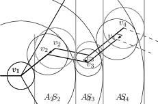
(b) Final transformation of the drawing.

Figure 6: Constructing the heavy path drawing by appending drawings of its heavy nodes.

Since each disk $D_{i}$ is placed in its own strip $S_{i}$, no two disks intersect (property 3) and since heavy edges are straight-line segments within two adjacent strips, they do not intersect any non-incident disks (property 1). The light edge $uv_{1}$ is completely to the left of all strips and thus does not intersect the drawing of $P$ (property 2). Since we were using the existing drawings (or their mirror images) of all heavy nodes, their perfect angular resolution is preserved (property 4).

The current drawing has a width that is equal to the sum of the diameters of the disks $D_{1},\ldots,D_{k}$. However, it does not yet necessarily fit into a disk $D$ centered at $v_{1}$ whose radius equals that sum of the diameters. To achieve this we create $k-1$ annuli $A_{2},\ldots,A_{k}$ centered around $v_{1}$, each $A_{i}$ of width $2r_{i}$. Then, for $i=2,\ldots,k$, we either shorten or extend the edge $v_{i-1}v_{i}$ until $D_{i}$ is contained in its annulus $A_{i}$; see Figure 6b. At each step $i$ we treat the remaining path $(v_{i},\ldots,v_{k})$ and its disks $D_{i},\ldots,D_{k}$ as a rigid structure that is translated as a whole and in parallel to the heavy edge $v_{i-1}v_{i}$; see the translation vectors indicated in Figure 6b. In the end, each disk $D_{i}$ is contained in its own annulus $A_{i}$ and thus all disks are still pairwise disjoint. Since we only stretch or shrink edges of an $x$-monotone path but do not change any edge directions, the whole transformation preserves the previous properties of the drawing. Clearly, all disks now lie inside a disk $D$ of radius $r=r_{1}+2\sum_{i=2}^{k}r_{i}\leq 2\sum_{i=1}^{k}r_{i}$ (property 5).

It remains to show the $O(k)$ time bound for drawing $P$. Here we store the coordinates of each $v_{i}$ in $P$ not only relative to the parent node $v_{i-1}$ but also relative to the root $v_{1}$ of $P$. Initially, each disk is placed in its vertical strip as shown in Figure 6a and the order of the children is selected as either clockwise or counterclockwise as needed. (Recall that changing the direction can be done in constant time.) Then for $i=2,\dots,k$ each disk $D_{i}$ is translated into its annulus $A_{i}$; see Figure 6b. In this process the coordinates of $v_{i}$ with respect to $v_{1}$ can become temporarily invalid but the coordinates relative to the predecessor node $v_{i-1}$ remain valid. Given the final position of $D_{i}$ in $A_{i}$ and the current position of $D_{i+1}$ with respect to $v_{i}$ we obtain the final position of $D_{i+1}$ in $A_{i+1}$, both with respect to $v_{1}$ and to $v_{i}$. The assignment of the coordinates for every node of $P$ thus takes $O(k)$ time.  

Combining Lemmas 2 and 3 yields the following theorem:

Theorem 1

Given an unordered tree $T$ with $n$ nodes we can find, in $O(n)$ time and space, a crossing-free straight-line drawing of $T$ with perfect angular resolution that fits inside a disk $D$ of radius $2\cdot 8^{h(T)}n$, where $h(T)$ is the height of the heavy-path decomposition of $T$. Since $h(T)\leq\log_{2}{n}$ the radius of $D$ is no more than $2n^{4}$.

Proof: From Lemma 2 we know that, for each node $v$ of a heavy path $P$ at level $j$, the radius of the disk $D$ containing $v$ and all its light subtrees is $r_{v}=8^{h(T)-j}l(v)$. Lemma 3 yields that $P=(v_{1},\dots,v_{k})$ and all its descendants can be drawn in a disk of radius $r=2\sum_{i=1}^{k}r_{v_{i}}=2\cdot 8^{h(T)-j}\sum_{i=1}^{k}l(v_{i})=2\cdot 8^{h(T)-j}n(P)$, where $n(P)$ is the number of nodes of $P$ and its descendants. This holds, in particular, for the heavy path $\hat{P}$ at the root of $H(T)$.

It remains to show the linear time and space bound. As indicated in Section 2.1 the heavy path decomposition is computed in linear time and has linear size. Since the drawing subroutines for nodes and heavy paths in Lemmas 2 and 3 both require linear time and are called only once for each node and heavy path, respectively, these steps take $O(n)$ time in total. In the final step we set the coordinates of the root of $T$ to $(0,0)$ and propagate the absolute positions of all nodes from top to bottom. Thus the entire process takes $O(n)$ time. As we only store a constant amount of information with each node of $T$, it follows that the space needed is also $O(n)$.  

Corollary 1

The drawing of $T$ according to Theorem 1 requires polynomial area.

Proof: Our first definition of area (the ratio of the area of the smallest enclosing disk over the square of the length of the shortest edge) yields an area value of at most $4\pi n^{8}$ for the drawing of $T$ since the shortest edges have length at least 1 and $D$ has radius at most $2n^{4}$. In the alternative notions of area defined by the (squared) ratio of the farthest distance of any two nodes (or edges) to the smallest distance of any two nodes (or non-adjacent edges) a similar polynomial area bound holds. Clearly the farthest distance in both cases is at most the diameter $4n^{4}$ of $D$. Furthermore, every child node in the drawing is contained in its own overlap-free disk of radius 1 and hence the closest pair of nodes has distance at least 1. For the closest pair of edges there is also a lower distance bound of 1. In every step of the recursive drawing procedure a subtree $T_{u}$ is drawn inside a disk $D_{u}$ with the property that there is an empty outer annulus of width at least 1 in $D_{u}$. When composing different subdrawings, this ensures that their edges are kept far enough apart. Thus it is easy to see by induction that no pair of edges can get closer than distance 1.  

3 Straight-line drawings for ordered trees

In many cases, the ordering of the children around each node of a tree is given; that is, the tree is ordered (or has a fixed combinatorial embedding). In the previous section we relied on the freedom to order subtrees as needed to achieve a polynomial area bound. Hence that algorithm cannot be applied to ordered trees with fixed embeddings. As we now show, there are ordered trees that have no straight-line crossing-free drawings with perfect angular resolution and polynomial area.

Specifically, we present a class of ordered trees for which any straight-line crossing-free drawing with perfect angular resolution requires exponential area. We define the 3-legged Fibonacci caterpillar of length $k$ to be an ordered caterpillar tree $T_{k}$, whose spine (the subgraph obtained after removing all leaves) is a $k$-node path $P=(p_{1},\dots,p_{k})$ in which every node $p_{i}$ has degree 5 in $T_{k}$, hence three legs. The embedding of $T_{k}$ specifies that in every node $p_{i}$ ($i=2,\dots,k-1$) the edge $p_{i}p_{i+1}$ is the immediate counterclockwise successor of $p_{i}p_{i-1}$. Hence in any straight-line drawing of $T_{k}$ with perfect angular resolution, the spine is represented as a simple polyline with $k-2$ right turns of $108^{\circ}$, forming a $72^{\circ}$ angle between adjacent edges; see Figure 7.

(a)

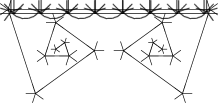
(b)

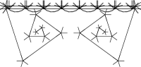
(c)

Figure 7: (a) A Fibonacci caterpillar; (b) Lombardi drawing; (c) Straight-line drawing with perfect angular resolution and exponential area.

We define a clockwise (counterclockwise) spiral to be a polyline $(q_{1},\dots,q_{k})$ such that for any index $3\leq i\leq k-1$ the polyline $(q_{1},\dots,q_{i})$ lies to the right (left) of the ray $\overrightarrow{q_{i}q_{i+1}}$. First, we show that any drawing of the Fibonacci caterpillar contains a large spiral.

Lemma 4

In any straight-line drawing with perfect angular resolution of $T_{k}$ the spine $P$ contains a spiral consisting of at least $k/2$ nodes.

Proof: For $k\leq 5$, because of the required fixed angle turns, either $P=(p_{1},\dots,p_{k})$ is a clockwise spiral or its reverse $\overline{P}=(p_{k},\dots,p_{1})$ is a counterclockwise spiral. So let $k>5$. For $i=1,\dots,k-1$ we abbreviate the edge $p_{i}p_{i+1}$ as $e_{i}$. We look at sequences $S_{i}$ of four consecutive edges $(e_{i},e_{i+1},e_{i+2},e_{i+3})$ of $P$ and distinguish two cases. If the extension of edge $e_{i+3}$ into a ray $\overrightarrow{p_{i+3}p_{i+4}}$ intersects $e_{i}$ or $e_{i+1}$, we say the sequence $S_{i}$ is locked, and otherwise we say it is open; see Figure 8. Starting from $i=1$ we scan the spine $P$ for the first occurrence $j$ of a locked sequence $S_{j}$. Then the prefix path $(p_{1},\dots,p_{j+3})$ is a clockwise spiral.

(a)

(b)

(c)

Figure 8: Two locked edge sequences (a) and (b) and an open sequence (c).

Furthermore, for any $i\geq j$ the sequence $S_{i}$ is also locked, as can be seen by induction. Let $S_{i}$ be a locked sequence. Then node $p_{i+5}$ lies inside the quadrilateral (or triangle) defined by edges $e_{i},e_{i+1},e_{i+2}$ and the ray $\overrightarrow{p_{i+3}p_{i+4}}$, and due to the angle of $72^{\circ}$ between $e_{i+3}$ and $e_{i+4}$ the ray $\overrightarrow{p_{i+4}p_{i+5}}$ must intersect either $e_{i+1}$ or $e_{i+2}$; see Figures 8a and 8b. This means that $S_{i+1}$ is also a locked sequence.

By observing that if a sequence $S_{i}=(e_{i},e_{i+1},e_{i+2},e_{i+3})$ is locked, then the reverse sequence $\overline{S_{i}}=(e_{i+3},e_{i+2},e_{i+1},e_{i})$ is open, the same reasoning as before yields that the suffix path $(p_{j},p_{j+1},\dots,p_{k})$ in reverse order $(p_{k},\dots,p_{j+1},p_{j})$ is a counterclockwise spiral. Clearly, one of the two spirals contains at least $k/2$ nodes.  

Now that we know that there is a large spiral in $T_{k}$ we show that drawing the spiral requires exponential area.

Lemma 5

The drawing of a spiral of length $n$ requires exponential area $\Omega(c^{n})$ for some $c>1$.

Proof: Without loss of generality we consider a path $P$ of length $n\geq 6$ that forms a clockwise spiral. Figure 9 shows the construction of a minimum-area drawing of $P$. Let the minimum length of any edge be $1$. We draw $e_{1}$ and $e_{2}$ with an angle of $72^{\circ}$ and length $1$ each. Every subsequent edge $e_{i}$ for $3\leq i\leq n-1$ is drawn just as long as necessary so that the sequence $S_{i}$ is open. Obviously, no edge can be shortened and increasing any edge only increases the area of the spiral.

Figure 9: Construction of a minimum-area spiral based on the angle $\alpha=72^{\circ}$.

This procedure creates a sequence of isosceles triangles $\Delta_{0},\dots,\Delta_{n-6}$ as indicated in Figure 9. Each $\Delta_{i}$ has two long sides of length $b_{i}$ and a short side of length $a_{i}$. The angles opposite the two long sides are $\alpha=72^{\circ}$ and the angle opposite the short side is $\beta=36^{\circ}$. By construction of the triangle sequence we obtain the recurrence $b_{i}=b_{i-3}+a_{i-4}$, which is similar to the definition of the Fibonacci numbers. From trigonometry we know that $a_{i}=\sin 36^{\circ}/\sin 72^{\circ}\cdot b_{1}=1/(2\cos 36^{\circ})\cdot b_{i}\approx 0.618\cdot b_{i}$ and that the area of $\Delta_{i}$ is $A_{i}=1/2\cdot b_{i}^{2}\sin 36^{\circ}$. Using $b_{i}=b_{i-3}+a_{i-4}\geq 2a_{i-4}$ and $a_{i}\geq a_{i-4}/\cos 36^{\circ}$ we can now bound $A_{i}$ as follows:

$$\begin{array}[]{rcl}A_{i}&=&\frac{1}{2}b_{i}^{2}\sin 36^{\circ}\\ &\geq&2\sin 36^{\circ}a_{i-4}^{2}\\ &\geq&2\sin 36^{\circ}\frac{1}{\cos 36^{\circ}}^{\lfloor i/4\rfloor}a_{0}\\ &\geq&1.236^{\lfloor i/4\rfloor}a_{0}.\end{array}$$ (1)

Clearly, the smallest disk containing the spiral has area at least $A_{n-6}$ and so by our definition of the area of a drawing the whole spiral has area $\Omega(c^{n})$ for $c=\sqrt[4]{1.236}\approx 1.054$.  

By combining Lemmas 4 and 5 we immediately obtain the following theorem since drawing the whole Fibonacci caterpillar $T_{k}$ requires at least as much area as drawing only its spine.

Theorem 2

Any straight-line drawing of the Fibonacci caterpillar $T_{k}$ with perfect angular resolution requires area $\Omega(c^{k})$ for some $c>1$.

Similar reasoning was used by Frati [16] to show an exponential lower bound on the area of upward straight-line drawings for ordered trees. The Fibonacci caterpillar shows that we cannot maintain all constraints (straight-line edges, crossing-free, perfect angular resolution, polynomial area) for ordered trees. However, as we show next, using circular arcs instead of straight-line edges allows us to respect the other three constraints; see Figure 7b.

4 Lombardi drawings for ordered trees

In this section, let $T$ be an ordered tree with $n$ nodes. As we have seen in Section 3, we cannot find polynomial area drawings for all ordered trees using straight-line edges. However, by using circular arc edges instead of straight-line segments we can achieve all remaining constraints as in the unordered case. That is, we can find crossing-free circular arc drawings with perfect angular resolution and polynomial area. Recall that a drawing with circular arcs and perfect angular resolution is called a Lombardi drawing [11].

The flavor of the algorithm for Lombardi tree drawings is similar to our straight-line tree drawing algorithm of Section 2: We first compute a heavy-path decomposition $H(T)$ for $T$, and then we recursively draw all heavy paths within disks of polynomial area in a bottom-up fashion. More precisely, we ensure the following invariant for the drawing of any heavy path and all its descendants.

Invariant 1

A heavy path $P$ at level $j$ of $H(T)$ and all its descendants are drawn inside a disk $D$ of radius $2\cdot 4^{h(T)-j}n(P)$, where $n(P)=|T_{v}|$ for the root $v$ of $P$.

Given the logarithmic height of the heavy path decomposition, this yields a drawing of $T$ with polynomial area.

In Section 4.1, we describe how to draw a heavy path $P$ (but not yet its light subtrees) under the assumption that each node of $P$ is centered in a disk of given radius. Subsequently, Section 4.2 shows how the light subtrees of a heavy-path node $v$, which are themselves heavy paths of the level below and thus recursively drawn within disks of fixed size according to Invariant 1, are placed within the space reserved around $v$ in the previous step. These two steps define the drawing of a heavy path $P$ and all its descendants, which we show satisfies Invariant 1, and which is then used as a component for the drawing of the parent of $P$ in $H(T)$.

4.1 Drawing heavy paths

Let $P=(v_{1},\ldots,v_{k})$ be a heavy path at level $j$ of the heavy-path decomposition. Since we will draw $P$ incrementally starting from the leaf and ending with the root of $P$, we assume that the last node $v_{k}$ is the root of $P$. We denote each edge $v_{i}v_{i+1}$ by $e_{i}$. Recall that the angle at an intersection point of two circular arcs is measured as the angle between the tangents to the arcs at that point. We define the angle $\alpha(v_{i})$ for $2\leq i\leq k-1$ to be the angle between $e_{i-1}$ and $e_{i}$ at node $v_{i}$ (measured counter-clockwise). The angle $\alpha(v_{k})$ is defined as the angle at $v_{k}$ between $e_{k-1}$ and the light edge $e=v_{k}u$ connecting the root $v_{k}$ of $P$ to its parent $u$. Due to the perfect angular resolution requirement for each node $v_{i}$, the angle $\alpha(v_{i})$ is obtained directly from the number of edges between $e_{i-1}$ and $e_{i}$ and the degree $d(v_{i})$.

Lemma 6

Given a heavy path $P=(v_{1},\ldots,v_{k})$ and a disk $D_{i}$ of radius $r_{i}$ for the drawing of each $v_{i}$ and its light subtrees, we can draw $P$ with each $v_{i}$ in the center of its disk $D_{i}$ inside a large disk $D$ in $O(k)$ time such that the following properties hold:

1. each heavy edge $e_{i}$ is a circular arc that does not intersect any disk other than $D_{i}$ and $D_{i+1}$;

2. there is a stub edge incident to $v_{k}$ that is reserved for the light edge connecting $v_{k}$ and its parent $u$;

3. any two disks $D_{i}$ and $D_{j}$ for $i\neq j$ are disjoint;

4. the angle between any two consecutive heavy edges $e_{i-1}$ and $e_{i}$ is $\alpha(v_{i})$;

5. the radius of $D$ is $r=2\sum_{i=1}^{k}r_{i}$.

Proof: We draw $P$ incrementally starting from the leaf $v_{1}$ by placing $D_{1}$ in the center $M$ of the disk $D$ of radius $r=2\sum_{i=1}^{k}r_{i}$. We may assume that $D_{1}$ is rotated such that the edge $e_{1}$ is tangent to a horizontal line at $v_{1}$ and that it leaves $v_{1}$ to the right. All disks $D_{2},\ldots,D_{k}$ will be placed with their centers $v_{2},\ldots,v_{k}$ on concentric circles $C_{2},\ldots,C_{k}$ around $M$ as shown in Figure 10. The radius of $C_{i}$ is $r_{1}+2\sum_{j=2}^{i-1}r_{j}+r_{i}$ so that $D_{i-1}$ and $D_{i}$ are placed in disjoint annuli separated by the circle $\hat{C}_{i-1}$ of radius $r_{1}+2\sum_{j=2}^{i-1}r_{j}$. Hence by construction no two disks intersect (property 3). Each disk $D_{i}$ will be rotated around its center such that the tangent to $C_{i}$ at $v_{i}$ is the bisector of the angle $\alpha(v_{i})$.

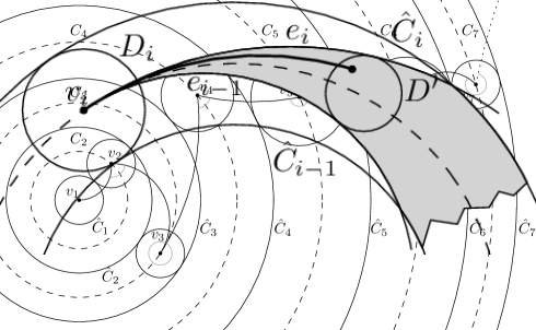
Figure 10: Drawing a heavy path $P$ on concentric circles with circular-arc edges. The angles $\alpha(v_{i})$ are marked in gray; the edge stub to connect $v_{7}$ to its parent is dotted.

We now describe one step in the iterative drawing procedure that draws edge $e_{i}$ and disk $D_{i+1}$ given a drawing of $D_{1},\ldots,D_{i}$. Disk $D_{i}$ is placed such that $C_{i}$ bisects the angle $\alpha(v_{i})$ and hence we immediately obtain the slope of the tangent to $e_{i}$ at $v_{i}$. This defines a family $\mathcal{F}_{i}$ of circular arcs emitted from $v_{i}$ with the same given tangent slope at $v_{i}$ that intersect the circle $C_{i+1}$; see Figure 11. We consider all arcs from $v_{i}$ until their first intersection point with $C_{i+1}$. Observe that the intersection angles of $\mathcal{F}_{i}$ and $C_{i+1}$ bijectively cover the full interval $[0,\pi]$, i.e., for any angle $\alpha\in[0,\pi]$ there is a unique arc in $\mathcal{F}_{i}$ that has intersection angle $\alpha$ with $C_{i+1}$. Hence we choose for $e_{i}$ the unique circular arc that realizes the angle $\alpha(v_{i+1})/2$ and place the center $v_{i+1}$ of $D_{i+1}$ at the endpoint of $e_{i}$. Since the centers of all arcs $a$ in $\mathcal{F}_{i}$ lie on a line $\ell_{i}$, we parameterize them as $a=a(t)$ by a parameter $t\in\mathbb{R}\cup\{\infty\}$ that yields the corresponding circle center on $\ell_{i}$. Then we consider the angle of the tangents to $a(t)$ and the circle $C_{i+1}$ in their first intersection point $p(t)$ and set it equal to $\alpha(v_{i+1})/2$. Solving this equation for $t$ requires finding the roots of a polynomial of bounded degree, which we assume to be possible in constant time. We store the resulting arc center and radius together with $e_{i}$. We continue this process until the last disk $D_{k}$ is placed. This drawing of $P$ realizes the angle $\alpha(v_{i})$ between any two heavy edges $e_{i-1}$ and $e_{i}$ (property 4). For the edge from $v_{k}$ to its parent $u$ we can only reserve a stub whose tangent at $v_{k}$ has a fixed slope (property 2). The only information that we have about the edge $v_{k}u$ is that it belongs to the family $\mathcal{F}_{k}$ of arcs that intersect the circle $\hat{C}_{k}$ and have the given tangent at $v_{k}$. This ambiguity does not cause problems in the subsequent steps though, and hence we can reserve all of the possible arcs simultaneously. Figure 10 shows an example.

Figure 11: Any angle $\alpha\in[0,\pi]$ can be realized.

Each edge $e_{i}$ is contained in the annulus between $C_{i}$ and $C_{i+1}$ and thus does not intersect any other edge of the heavy path or any disk other than $D_{i}$ and $D_{i+1}$ (property 1). Furthermore, the disk $D$ with radius $r=2\sum_{i=1}^{k}r_{i}$ indeed contains all the disks $D_{1},\ldots,D_{k}$ (property 5).

It remains to show the time bound for computing the drawing of $P$. Similarly to drawing heavy paths in Section 2, we store the position of each node $v_{i}$ in polar coordinates relative to its predecessor and relative to the center $M$ of $D$. This avoids the need to update the positions of all descendants in every step and allows to assign the final absolute coordinates in a top-down traversal of $T$. Given the position of node $v_{i}$ (with respect to $M$) we can compute the position of $v_{i+1}$ with respect to $M$ in constant time as described above. Once all nodes of $P$ are placed, we additionally set the coordinates of each node $v_{i}$ with respect to its parent $v_{i+1}$. The required time is $O(k)$.  

Lemma 6 showed how to draw a heavy path $P$ with prescribed angles between the heavy edges and an edge stub to connect it to its parent. Since the root $v$ of each heavy path $P$ (except the path at the root of $H(T)$) is the light child of a node on the previous level of $H(T)$, the light edge from $v$ to its parent is actually drawn when placing the light subtrees of a node, the topic of the next subsection.

4.2 Drawing light subtrees

Once the heavy path $P$ is drawn as described above, it remains to place the light subtrees of each node $v_{i}$ of $P$. For each node $v_{i}$ the two heavy edges incident to it partition the disk $D_{i}$ into two regions. We call the region that contains the larger conjugate angle the large zone of $v_{i}$ and the region that contains the smaller conjugate angle the small zone. If both angles are equal to $\pi$, then we can consider both regions as small zones. For the root node $v_{k}$ of $P$ we only know one heavy edge to $v_{k-1}$, whereas the light edge to its parent $u$ is not yet fully determined. In this case we define the two zones of $v_{k}$ as the regions between the heavy edge and the leftmost/rightmost possible arc for the light edge $v_{k}u$. Since the light subtrees of $v_{k}$ will be placed in the small and large zones of $v_{k}$, the node $v_{k}$ can always be connected to its parent $u$ by an arc that does not intersect any edge in $T_{v_{k}}$. We say that $v_{k}$ is exposed to its parent. Our approach in this section proceeds in two steps. First, we find a disjoint placement of the child disks in the small and large zone. In the second step, we actually draw the light edges from $v_{i}$ to all its light children.

For a node $v_{i}$ at level $j$ of $H(T)$ we define the radius $r_{i}$ of $D_{i}$ as $r_{i}=4^{h(T)-j}(1+\sum_{u\in L(v_{i})}|T_{u}|)=4^{h(T)-j}l(v_{i})$. All light children of $v_{i}$ are at level $j+1$ of $H(T)$ and thus by inductively assuming that Invariant 1 holds, every light child $u$ of $v_{i}$ and its subtree is drawn in a disk of radius $r_{u}=2\cdot 4^{h(T)-j-1}|T_{u}|$. Thus we know that $r_{u}\leq r_{i}/2$; in fact, we even have $\sum_{u\in L(v_{i})}r_{u}\leq r_{i}/2$.

Light subtrees in the small zone.

Depending on the angle $\alpha(v_{i})$, the small zone of a disk $D_{i}$ might actually be too narrow to directly place the light subtrees in it. Therefore, we define the extended small zone as the area bounded by $e_{i-1}$, $e_{i}$, $\hat{C}_{i-1}$, $\hat{C}_{i}$, and the horizontal ray to $-\infty$ through $v_{1}$. Fortunately, we can always place another disk $D^{\prime}$ of radius at most $r_{i}/2$ in this extended small zone such that $D^{\prime}$ touches $e_{i-1}$ and $e_{i}$ and does not intersect any other previously placed disk; see Figure 12. For a given radius of $D^{\prime}$ the position of the center of $D^{\prime}$ with respect to $v_{i}$ can be computed in constant time. If there is a single child $u$ in the small zone then $D^{\prime}=D_{u}$ and we are done. The next lemma shows how to place more than one child. Let $l\geq 2$ be the number of light children of $v_{i}$ to be placed in the (extended) small zone. We say that the disks $D^{\prime}_{1},\dots,D^{\prime}_{l}$ are correctly placed in the (extended) small zone if their interiors are mutually disjoint and if every point inside any disk $D^{\prime}_{i}$ can be reached by a circular arc from $v_{i}$ with given slope at $v_{i}$ such that the arc does not intersect any other disk $D^{\prime}_{j}$ for $j\neq i$.

Figure 12: Placing a single disk $D^{\prime}$ in the extended small zone of $D_{i}$ (shaded gray).

Lemma 7

If a single disk $D^{\prime}$ of radius $r^{\prime}$ can be placed in the (possibly extended) small zone of the disk $D_{i}$, then we can correctly place any sequence of $l$ disks $D^{\prime}_{1},\ldots,D^{\prime}_{l}$ with radii $r_{1}^{\prime},\ldots,r_{l}^{\prime}$ and $\sum_{i=1}^{l}r_{i}^{\prime}=r^{\prime}$ in the (extended) small zone of $D_{i}$. This can be done in $O(l)$ time.

Proof: The idea of the algorithm for placing the $l$ disks is to first place the disk $D^{\prime}$ in the small zone as before. The disks $D^{\prime}_{1},\ldots,D^{\prime}_{l}$ will then be placed within $D^{\prime}$ so that no additional space is required.

In the first step of the recursive placement algorithm we either place $D^{\prime}_{1}$ or $D^{\prime}_{l}$ (whichever has smaller radius) and a disk $D^{\prime\prime}$ containing the remaining sequence of disks $D^{\prime}_{2},\ldots,D^{\prime}_{l}$ or $D^{\prime}_{1},\ldots,D^{\prime}_{l-1}$, respectively. Without loss of generality, let $r_{1}^{\prime}\leq r_{l}^{\prime}$ and thus in particular $r_{1}^{\prime}\leq r^{\prime}/2$. In order to fit inside $D^{\prime}$ the disks $D^{\prime}_{1}$ and $D^{\prime\prime}$ must be placed with their centers on a diameter of $D^{\prime}$; see Figure 13a. The degree of freedom that we have is the rotation of that diameter around the center of $D^{\prime}$. Then the locus of the tangent point of $D^{\prime}_{1}$ and $D^{\prime\prime}$ is a circle $\hat{C}$ of radius $r^{\prime}-2r_{1}^{\prime}$ around the center of $D^{\prime}$; see Figure 13b. For any given tangent slope at $v_{i}$, in particular the slope required for the edge from $v_{i}$ to the light child in $D^{\prime}_{1}$, there are exactly two circular arcs $a_{1}$ and $a_{2}$ that are tangent to $\hat{C}$. They can be computed in constant time. Let the two points of tangency on $\hat{C}$ be $p_{1}$ and $p_{2}$. Now we rotate $D^{\prime}_{1}$ and $D^{\prime\prime}$ such that their point of tangency coincides with either $p_{1}$ or $p_{2}$ depending on which of them yields the correct embedding order of $D^{\prime}_{1}$ and $D^{\prime\prime}$ around $v_{i}$. Clearly, $a_{1}$ or $a_{2}$ are also tangent to $D^{\prime}_{1}$ and $D^{\prime\prime}$ now. Assume we choose $p_{1}$ and the corresponding arc $a_{1}$ as in Figure 13b. We claim that we can connect any point in $D^{\prime}_{1}$ to $v_{i}$ with the unique circular arc of the required slope at node $v_{i}$ without creating any edge crossings. (We will describe the exact placement of that arc later.) As in the proof of Lemma 6, there is a family $\cal F$ of circular arcs that pass through $v_{i}$ with the given slope. We consider the subset $\mathcal{F}^{\prime}\subset\mathcal{F}$ that intersects disk $D^{\prime}_{1}$ and thus can be used as basis for the edge from $v_{i}$ to the light child in $D^{\prime}_{1}$. Any such arc stays inside the horn-shaped region $\Upsilon$ that encloses $D^{\prime}_{1}$ and is formed by a boundary arc $b$ of the small zone and $a_{1}$ before it reaches $D^{\prime}_{1}$. Assume to the contrary that there is an arc $a\in\mathcal{F}^{\prime}$ that does not completely lie inside $\Upsilon$ before reaching $D^{\prime}_{1}$. The arc $a$ cannot intersect $a_{1}$ in a point other than $v_{1}$ since both $a$ and $a_{1}$ belong to $\cal F^{\prime}$. So $a$ must intersect the other boundary arc $b$ of $\Upsilon$. However, since $a$ intersects $b$ in $v_{i}$ and lies inside $\Upsilon$ in some $\varepsilon$-neighborhood of $v_{i}$ it would have to intersect $b$ at least three times in order to reach a point of $D^{\prime}_{1}\subset\Upsilon$. This is a contradiction. Since $a_{1}$ separates $D^{\prime}_{1}$ from $D^{\prime\prime}$, none of the arcs in $\cal F^{\prime}$ nor $D^{\prime}_{1}$ can interfere with any of the disks $D^{\prime}_{2},\ldots,D^{\prime}_{l}$ and their respective edges as long as those disks stay inside $D^{\prime\prime}$ or the edges connect to points in $D^{\prime\prime}$.

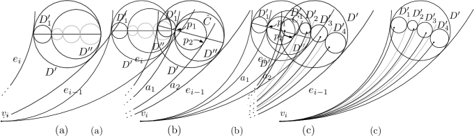
Figure 13: Placing disks $D^{\prime}_{1}$ and $D^{\prime\prime}$ inside the disk $D^{\prime}$.

For placing $D^{\prime}_{2},\ldots,D^{\prime}_{l}$ we recursively apply the same procedure again, now using $D^{\prime\prime}$ as the disk $D^{\prime}$ and $a_{1}$ as one of the boundary arcs. Then after $l$ steps, we have disjointly placed all disks $D^{\prime}_{1},\ldots,D^{\prime}_{l}$ inside the disk $D^{\prime}$ such that their order respects the given tree order and no two edges can possibly intersect. In other words they are correctly placed and each step can be performed in constant time. Figure 13c gives an example.  

We required that the edges $e_{i-1}$ and $e_{i}$ are tangent to $D^{\prime}$, which is possible only for an opening angle $\alpha$ of the small zone of at most $\pi$. For any angle $\alpha\leq\pi$ the arcs $a_{1}$ and $a_{2}$ always stay within the extended small zone and form at most a semi-circle. This does not hold for $\alpha>\pi$.

Light subtrees in the large zone.

Placing the light subtrees of a node $v_{i}$ in the large zone of $D_{i}$ must be done slightly different from the algorithm for the small zone since Lemma 7 holds only for opening angles of at most $\pi$. On the other hand, the large zone does not become too narrow and there is no need to extend it beyond $D_{i}$. Our approach splits the large zone incident to the heavy-path node $v_{i}$ into two parts that again have an opening angle of at most $\pi$ so that we can apply Lemma 7 and draw all the children of $v_{i}$ accordingly.

Let $l$ be the number of light subtrees in the large zone of $D_{i}$. We first place a disk $D^{\prime}$ of radius at most $r_{i}/2$ that touches $v_{i}$ and whose center lies on the line bisecting the opening angle of the large zone. The disk $D^{\prime}$ is large enough to contain the disjoint disks $D^{\prime}_{1},\ldots,D^{\prime}_{l}$ for the light subtrees of $v_{i}$ along its diameter. We need to distinguish whether $l$ is even or odd. For even $l$ we create a container disk $D^{\prime\prime}_{1}$ for disks $D^{\prime}_{1},\ldots,D^{\prime}_{l/2}$ and a container disk $D^{\prime\prime}_{2}$ for $D^{\prime}_{l/2+1},\ldots,D^{\prime}_{l}$. Now $D^{\prime\prime}_{1}$ and $D^{\prime\prime}_{2}$ can be tightly packed on the diameter of $D^{\prime}$. Using a similar argument as in Lemma 7 we separate the two disks by a circular arc through $v_{i}$ that is tangent to the bisector of $\alpha(v_{i})$ in $v_{i}$. Since $D^{\prime}$ is centered on the bisector this is possible even though the actual opening angle of the large zone is larger than $\pi$. If $l$ is odd, we create a container disk $D^{\prime\prime}_{1}$ for disks $D^{\prime}_{1},\ldots,D^{\prime}_{\lfloor l/2\rfloor}$ and a container disk $D^{\prime\prime}_{2}$ for $D^{\prime}_{\lceil l/2\rceil+1},\ldots,D^{\prime}_{l}$. The median disk $D^{\prime}_{\lceil l/2\rceil}$ is not included in any container. Then we apply Lemma 7 to $D^{\prime}$ and the three disks $D^{\prime\prime}_{1},D^{\prime}_{\lceil l/2\rceil},D^{\prime\prime}_{2}$ along the diameter of $D^{\prime}$; see Figure 14a. The separating circular arcs in $v_{i}$ are again tangent to the bisector of $\alpha(v_{i})$, which is, since $l$ is odd, also the correct slope for the circular arc connecting $v_{i}$ to the median disk $D^{\prime}_{\lceil l/2\rceil}$.

In both cases we split the large zone and the sequence of light subtrees to be placed into two parts that each have an opening angle at $v_{i}$ of at most $\pi$ between a separating circular arc and the edge $e_{i-1}$ or $e_{i}$, respectively. Next, we move $D^{\prime\prime}_{1}$ and $D^{\prime\prime}_{2}$ along the separating circular arcs keeping their tangencies until they also touch the edge $e_{i-1}$ or $e_{i}$, respectively. Then we can apply Lemma 7 to both container disks and thus place all light subtrees in the large zone; see Figure 14b. The splitting of the large zone involves finding tangent arcs to at most three disks and thus takes constant time. Combining this with the running time in Lemma 7 for the two small subinstances all $l$ disks in the large zone can be placed in $O(l)$ time.

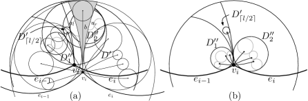
Figure 14: Placing light subtrees in the large zone by first splitting it into two parts (a) and then applying the algorithm for small zones to each part (b).

Drawing light edges

The final missing step is how to actually connect a heavy node $v_{i}$ to its light children given a position of $v_{i}$ and positions with respect to $v_{i}$ of all disks containing the light subtrees of $v_{i}$. Let $u$ be a light child of $v_{i}$ and let $D_{u}$ be the disk containing the drawing of $T_{u}$. When placing the disk $D_{u}$ in the small or large zone of $v_{i}$ we made sure that a circular arc from $v_{i}$ with the tangent required for perfect angular resolution at $v_{i}$ can reach any point inside $D_{u}$ without intersecting another edge or disk.

On the other hand, we know by Lemma 6 that $u$ is placed in the outermost annulus of $D_{u}$ and that it has reserved a stub for the edge $e=uv_{i}$. This stub represents all arcs in $u$ that share the tangent for $e$ required to obtain perfect angular resolution in $u$. Let $C_{u}$ be the circle that is the locus of $u$ if we rotate $D_{u}$ and the drawing of $T_{u}$ around the center of $D_{u}$.

There is again a family $\mathcal{F}$ of circular arcs with the required tangent at $v_{i}$ that all lead towards $D_{u}$ and intersect the circle $C_{u}$. As observed in Lemma 6 the intersection angles formed between $\mathcal{F}$ and $C_{u}$ bijectively cover the full interval $[0,\pi]$, i.e., for any angle $\alpha\in[0,\pi]$ there is a unique circular arc in $\mathcal{F}$ that has an intersection angle of $\alpha$ with $C_{u}$. In order to correctly attach $u$ to $v_{i}$ we first compute the arc $a$ in $\mathcal{F}$ that realizes an intersection angle of $\alpha(u)/2$ with $C_{u}$, where $\alpha(u)$ is the angle between $e$ and the heavy edge from $u$ to its heavy child that is required for perfect angular resolution at $u$. This arc $a$ can be computed in constant time similarly to computing a heavy-path edge in Lemma 6. Let $p$ be the intersection point of $a$ with $C_{u}$. Then we rotate $D_{u}$ and the drawing of $T_{u}$ around the center of $D_{u}$ until $u$ is placed at $p$; see node $v_{7}$ in Figure 10. This rotation is actually realized by setting the coordinates of $u$ with respect to its parent $v_{i}$ to those of $p$. We also store with $u$ the rotation angle between the new position of $D_{u}$ and its neutral position. Since the stub of $u$ for $e$ also has an angle of $\alpha(u)/2$ with $C_{u}$, the arc $a$ indeed realizes the edge $e$ with the required angles for perfect angular resolution in both $u$ and $v_{i}$. Furthermore, $a$ does not enter the disk bounded by $C_{u}$ and hence it does not intersect any part of the drawing of $T_{u}$ other than $u$.

We can summarize our results for drawing the light subtrees of a node as follows:

Lemma 8

Let $v$ be a node of $T$ at level $j$ of $H(T)$ with two incident heavy edges. For every light child $u\in L(v)$ assume there is a disk $D_{u}$ of radius $r_{u}=2\cdot 4^{h(T)-j-1}|T_{u}|$ that contains a fixed drawing of $T_{u}$ with perfect angular resolution and such that $u$ is exposed to its parent $v$. Then we can construct in $O(d(v))$ time a drawing of $v$ and its light subtrees inside a disk $D$, potentially with an extended small zone, such that the following properties hold:

1. the edge between $v$ and any light child $u\in L(v)$ is a circular arc that does not intersect any disk other than $D_{u}$;

2. the heavy edges do not intersect any disk $D_{u}$;

3. any two disks $D_{u}$ and $D_{u^{\prime}}$ for $u\neq u^{\prime}$ are disjoint;

4. the angular resolution of $v$ is $2\pi/d(v)$;

5. the disk $D$ has radius $r_{v}=4^{h(T)-j}l(v)$.

Now we have all ingredients for drawing the entire tree $T$ based on its heavy-path decomposition. We combine Lemmas 6 and 8 to recursively obtain a Lombardi drawing of $T$ in a bottom-up fashion. In the final step, we set the coordinates of the root of $T$ to $(0,0)$ and propagate the absolute node and edge positions downward using the relative positions and rotation angles stored during the recursive calls. We conclude with the following theorem:

Theorem 3

Given an ordered tree $T$ with $n$ nodes we can find in $O(n)$ time and space a crossing-free Lombardi drawing of $T$ that preserves the embedding of $T$ and fits inside a disk $D$ of radius $2\cdot 4^{h(T)}n$, where $h(T)$ is the height of the heavy-path decomposition of $T$. Since $h(T)\leq\log_{2}n$ the radius of $D$ is no more than $2n^{3}$.

Corollary 2

The drawing of $T$ according to Theorem 3 requires polynomial area.

Proof: Since the shortest edges have again length at least 1, Theorem 3 implies that the area of the Lombardi drawing of $T$ is at most $4\pi n^{6}$ according to our first area measure. Exactly the same arguments as used in Corollary 1 yield again that the polynomial area bounds continue to hold for the two alternative definitions of area based on the (squared) distance ratio of the farthest pair of nodes (or edges) to the closest pair of nodes (or non-adjacent edges), where in this case the farthest pair has distance at most $4n^{3}$ and the closest pair again at least distance $1$.  

Figure 2b shows a drawing of the ordered tree in Figure 3 according to our method. Instead of asking for perfect angular resolution, the same algorithm can also be used to construct a circular-arc drawing of an ordered tree with an arbitrary given assignment of angles between consecutive edges around each node that add up to $2\pi$. The drawing remains crossing-free and fits inside a disk of radius $O(n^{3})$.

5 Implementation Details

Since tree drawings with perfect angular resolution are also of practical importance, we have implemented a basic version of our straight-line drawing algorithm. The algorithm, whose area is polynomially bounded, from a practical viewpoint is still far from desirable. In particular, as Figure 15a illustrates, there is significant space left between sibling nodes. As Figure 15b demonstrates, with some simple heuristical refinements, far better use of space can be achieved.

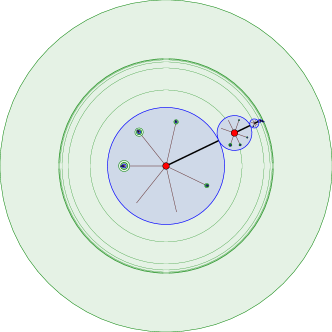
(a) Layout drawn by the unmodified straight-line tree drawing algorithm. Although polynomially bounded, the area is so large that smaller features of the drawing are difficult to see.

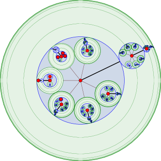
(b) A space-optimized drawing that still maintains the stated guarantees.

Figure 15: A partial snapshot of a tree drawing.

We highlight a few straightforward space-saving improvements to the algorithm that still ensure the same area bound. In the original construction, only large nodes are placed on the outer region with the smaller nodes placed inside the inner annulus. By continuing with a greedy approach of repeatedly inserting the next largest node in the outer region, skipping the spoke associated with the heavy edge, until no more nodes fit, and filling the remaining spokes with the smaller children, we can insert more nodes into the outer region. Moreover, the radii for many of the subtrees are far smaller than necessary. After laying out the positions of each of the light subtrees, we increase their radii so their disk fits maximally within their wedge region, thus using considerably more of the allocated space. Noting that the heavy path also does not completely fill the disk associated with its head node, we also increase this radius as a constant factor after having laid out the main drawing. Figures 16 and 17 provide further illustrations of these improvements.

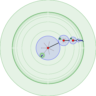
(a) Partial layout drawn by the unmodified straight-line tree drawing algorithm that places only large nodes in the outside annulus.

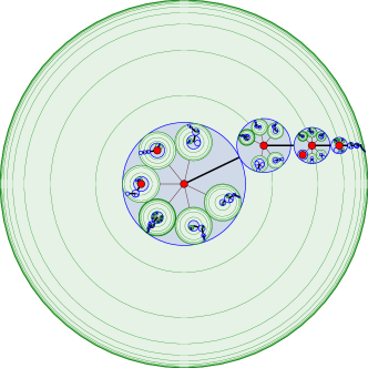
(b) The same tree but with space-filling optimization in place.

Figure 16: A partial snapshot of a tree drawing demonstrating filling the disk associated with the light subtree.

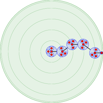
(a) The Fibonacci caterpillar drawn as an unordered tree.

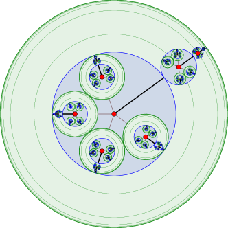
(b) A 5-ary tree with different weight distributions per child.

Figure 17: Example illustrations.

6 Conclusion and Closing Remarks

We have shown that straight-line drawings of trees with perfect angular resolution and polynomial area can be efficiently computed, by carefully ordering the children of each node and by using a style similar to balloon drawings in which the children of any node are placed on two concentric circles rather than on a single circle. However, using our Fibonacci caterpillar example we also showed that this combination of straight-line edges, perfect angular resolution, and polynomial area can no longer be achieved if the order of the children of each node is fixed. Fortunately, for ordered trees with a fixed embedding, Lombardi drawings (in which edges are drawn as circular arcs) allow us to retain the other desirable qualities of absence of crossings, polynomial area, and perfect angular resolution.

In addition to needing to implement the algorithm for an ordered tree, there remain further improvements to the basic implementation for the unordered tree discussed in Section 5. Since our intent was to highlight the key heavy path breakdown in our algorithm, even when the heavy child could fit as one of the node’s light children, we opted to place the heavy child separately, requiring more space than generally necessary.

Several problems in the study of Lombardi drawings of trees remain open. For example, our polynomial area bounds are likely not tight. In fact, recently Halupczok and Schulz [21] showed that any unordered $n$-node tree can be drawn within a disk of radius $n^{3.0367}$ using straight-line edges with perfect angular resolution. Moreover, our method is impractically complex. It would be of interest to find simpler Lombardi drawing algorithms that achieve perfect angular resolution for more limited classes of trees, such as binary trees, with better area bounds. Finally, there are many open problems in the area of plane Lombardi drawings of planar graphs.

Acknowledgments

This research was supported in part by the National Science Foundation under grants CCF-0545743, CCF-1115971 and CCF-0830403, by the Office of Naval Research under MURI grant N00014-08-1-1015, and by the German Research Foundation under grant NO 899/1-1.

References

- [1] U. Brandes and D. Wagner. Using graph layout to visualize train interconnection data. J. Graph Algorithms Appl. 4(3):135–155, 2000, doi:10.7155/jgaa.00028.
- [2] C. Buchheim, M. Jünger, and S. Leipert. Improving Walker’s algorithm to run in linear time. Proc. 10th Int. Symp. Graph Drawing (GD 2002), pp. 344–353. Springer-Verlag, LNCS 2528, 2002, doi:10.1007/3-540-36151-0_32.
- [3] J. Cappos, A. Estrella-Balderrama, J. J. Fowler, and S. G. Kobourov. Simultaneous graph embedding with bends and circular arcs. Computational Geometry 42(2):173–182, 2009, doi:10.1016/j.comgeo.2008.05.003.
- [4] J. Carlson and D. Eppstein. Trees with convex faces and optimal angles. Proc. 14th Int. Symp. Graph Drawing (GD 2006), pp. 77–88. Springer-Verlag, LNCS 4372, 2007, doi:10.1007/978-3-540-70904-6_9, arXiv:cs.CG/0607113.
- [5] T. Chan, M. T. Goodrich, S. R. Kosaraju, and R. Tamassia. Optimizing area and aspect ratio in straight-line orthogonal tree drawings. Computational Geometry 23(2):153–162, 2002, doi:10.1016/S0925-7721(01)00066-9.
- [6] C. C. Cheng, C. A. Duncan, M. T. Goodrich, and S. G. Kobourov. Drawing planar graphs with circular arcs. Discrete Comput. Geom. 25(3):405–418, 2001, doi:10.1007/s004540010080.
- [7] M. Dickerson, D. Eppstein, M. T. Goodrich, and J. Meng. Confluent drawings: Visualizing non-planar diagrams in a planar way. J. Graph Algorithms Appl. 9(1):31–52, 2005, doi:10.7155/jgaa.00099.
- [8] C. A. Duncan, A. Efrat, S. G. Kobourov, and C. Wenk. Drawing with fat edges. Int. J. Found. Comput. Sci. 17(5):1143–1164, 2006, doi:10.1142/S0129054106004315.
- [9] C. A. Duncan, D. Eppstein, M. T. Goodrich, S. G. Kobourov, and M. Löffler. Planar and poly-arc Lombardi drawings. Proc. 19th Int. Symp. Graph Drawing (GD 2011), pp. 308–319. Springer-Verlag, LNCS 7034, 2012, doi:10.1007/978-3-642-25878-7_30, arXiv:1109.0345.
- [10] C. A. Duncan, D. Eppstein, M. T. Goodrich, S. G. Kobourov, and M. Nöllenburg. Drawing trees with perfect angular resolution and polynomial area. Proc. 18th Int. Symp. Graph Drawing (GD 2010), pp. 183–194. Springer-Verlag, LNCS 6502, 2011, doi:10.1007/978-3-642-18469-7_17, arXiv:1009.0581.
- [11] C. A. Duncan, D. Eppstein, M. T. Goodrich, S. G. Kobourov, and M. Nöllenburg. Lombardi drawings of graphs. J. Graph Algorithms and Applications 16(1):85–108, 2012, doi:10.7155/jgaa.00251.
- [12] P. Eades. Drawing free trees. Bull. Inst. Combinatorics and Its Applications 5:10–36, 1992.
- [13] D. Eppstein. The graphs of planar soap bubbles. ArXiv e-prints, 2012, arXiv:1207.3761.
- [14] D. Eppstein. Planar Lombardi drawings for subcubic graphs. Proc. 20th Int. Symp. Graph Drawing (GD 2012). Springer-Verlag, LNCS, 2013, arXiv:1206.6142. To appear.
- [15] B. Finkel and R. Tamassia. Curvilinear graph drawing using the force-directed method. Proc. 12th Int. Symp. Graph Drawing (GD’04), pp. 448–453. Springer-Verlag, LNCS 3383, 2004, doi:10.1007/978-3-540-31843-9_46.
- [16] F. Frati. On minimum area planar upward drawings of directed trees and other families of directed acyclic graphs. Int’l J. Comput. Geom. & Appl. 18(3):251–271, 2008, doi:10.1142/S021819590800260X.
- [17] A. Garg, M. T. Goodrich, and R. Tamassia. Planar upward tree drawings with optimal area. Int. J. Comput. Geom. Appl. 6(3):333–356, 1996, doi:10.1142/S0218195996000228.
- [18] A. Garg and A. Rusu. Area-efficient order-preserving planar straight-line drawings of ordered trees. Int. J. Comput. Geom. Appl. 13(6):487–505, 2003, doi:10.1142/S021819590300130X.
- [19] A. Garg and A. Rusu. Straight-line drawings of binary trees with linear area and arbitrary aspect ratio. J. Graph Algorithms Appl. 8(2):135–160, 2004, doi:10.7155/jgaa.00086.
- [20] S. Grivet, D. Auber, J. P. Domenger, and G. Melançon. Bubble tree drawing algorithm. Proc. Int. Conf. Computer Vision and Graphics, pp. 633–641. Springer-Verlag, 2004, http://www.labri.fr/publications/is/2004/GADM04.
- [21] I. Halupczok and A. Schulz. Pinning balloons with perfect angles and optimal area. Proc. 19th Int. Symp. Graph Drawing (GD 2011), pp. 154–165. Springer-Verlag, LNCS 7034, 2011, doi:10.1007/978-3-642-25878-7_16.
- [22] D. Harel and R. E. Tarjan. Fast algorithms for finding nearest common ancestors. SIAM J. Comput. 13(2):338–355, 1984, doi:10.1137/0213024.
- [23] R. Hobbs and M. Lombardi. Mark Lombardi: Global Networks. Independent Curators International, New York, 2003.
- [24] C.-C. Lin and H.-C. Yen. On balloon drawings of rooted trees. J. Graph Algorithms Appl. 11(2):431–452, 2007, doi:10.7155/jgaa.00153.
- [25] M. Löffler and M. Nöllenburg. Planar Lombardi drawings of outerpaths. Proc. 20th Int. Symp. Graph Drawing (GD 2012). Springer-Verlag, LNCS, 2013. To appear.
- [26] G. Melançon and I. Herman. Circular Drawings of Rooted Trees. Tech. Rep. INS-R9817, CWI Amsterdam, 1998.
- [27] H. C. Purchase, J. Hamer, M. Nöllenburg, and S. G. Kobourov. On the usability of Lombardi graph drawings. Proc. 20th Int. Symp. Graph Drawing (GD 2012). Springer-Verlag, LNCS, 2012. To appear.
- [28] E. M. Reingold and J. S. Tilford. Tidier drawings of trees. IEEE Trans. Software Engineering 7(2):223–228, 1981, doi:10.1109/TSE.1981.234519.
- [29] C.-S. Shin, S. K. Kim, and K.-Y. Chwa. Area-efficient algorithms for straight-line tree drawings. Computational Geometry 15(4):175–202, 2000, doi:10.1016/S0925-7721(99)00053-X.
- [30] J. Walker. A node-positioning algorithm for general trees. Software Practice and Experience 20(7):685–705, 1990, doi:10.1002/spe.4380200705.
- [31] C. Wetherell and A. Shannon. Tidy drawings of trees. IEEE Trans. Software Engineering 5(5):514–520, 1979, doi:10.1109/TSE.1979.234212.
- [32] K. Xu, C. Rooney, P. Passmore, and D.-H. Ham. A user study on curved edges in graph visualization. Proc. IEEE Information Visualization Conference (InfoVis 2012), 2012. To appear.